Stochastic C-stability and B-consistency of explicit and implicit Milstein-type schemes

Abstract.

This paper focuses on two variants of the Milstein scheme, namely the split-step backward Milstein method and a newly proposed projected Milstein scheme, applied to stochastic differential equations which satisfy a global monotonicity condition. In particular, our assumptions include equations with super-linearly growing drift and diffusion coefficient functions and we show that both schemes are mean-square convergent of order $1$. Our analysis of the error of convergence with respect to the mean-square norm relies on the notion of stochastic C-stability and B-consistency, which was set up and applied to Euler-type schemes in [Beyn, Isaak, Kruse, J. Sci. Comp., 2015]. As a direct consequence we also obtain strong order $1$ convergence results for the split-step backward Euler method and the projected Euler-Maruyama scheme in the case of stochastic differential equations with additive noise. Our theoretical results are illustrated in a series of numerical experiments.

1. Introduction

More than four decades ago Grigori N. Milstein proposed a new numerical method for the approximate integration of stochastic ordinary differential equations (SODEs) in [15] (see [16] for an English translation). This scheme is nowadays called the Milstein method and offers a higher order of accuracy than the classical Euler-Maruyama scheme. In fact, G. N. Milstein showed that his method converges with order $1$ to the exact solution with respect to the root mean square norm under suitable conditions on the coefficient functions of the SODE while the Euler-Maruyama scheme is only convergent of order $\frac{1}{2}$, in general.

In its simplest form, that is for scalar stochastic differential equations driven by a scalar Wiener process $W$, the Milstein method is given by the recursion

(1) $$\begin{split}X_{h}(t+h)&=X_{h}(t)+hf(t,X_{h}(t))+g(t,X_{h}(t))\Delta_{h}W(t)\\ &\quad+\frac{1}{2}\big{(}\frac{\partial g}{\partial x}\circ g\big{)}(t,X_{h}(t))\big{(}\Delta_{h}W(t)^{2}-h\big{)},\end{split}$$

where $h$ denotes the step size, $\Delta_{h}W(t)=W(t+h)-W(t)$ is the stochastic increment, and $f$ and $g$ are the drift and diffusion coefficient functions of the underlying SODE (Equation (3) below shows the SODE in the full generality considered in this paper).

Since the derivation of the Milstein method in [15] relies on an iterated application of the Itō formula, the error analysis requires the boundedness and continuity of the coefficient functions $f$ and $g$ and their partial derivatives up to the fourth order. Similar conditions also appear in the standard literature on this topic [9, 17, 18].

In more recent publications these conditions have been relaxed: For instance in [10] it is proved that the strong order $1$ result for the scheme (1) stays true if the coefficient functions are only two times continuously differentiable with bounded partial derivatives, provided the exact solution has sufficiently high moments and the mapping $x\mapsto(\frac{\partial g}{\partial x}\circ g)(t,x)$ is globally Lipschitz continuous for every $t\in[0,T]$. On the other hand, from the results in [7] it follows that the explicit Euler-Maruyama method is divergent in the strong and weak sense if the coefficient functions are super-linearly growing. Since the same reasoning also applies to the Milstein scheme (1) it is necessary to consider suitable variants in this situation.

One possibility to treat super-linearly growing coefficient functions is proposed in [23]. Here the authors combine the Milstein scheme with the taming strategy from [8]. This allows to prove the strong convergence rate $1$ in the case of SODEs whose drift coefficient functions satisfy a one-sided Lipschitz condition. The same approach is used in [12], where the authors consider SODEs driven by Lèvy noise. However, both papers still require that the diffusion coefficient functions are globally Lipschitz continuous.

This is not needed for the implicit variant of the Milstein scheme considered in [6], where the strong convergence result also applies to certain SODEs with super-linearly growing diffusion coefficient functions. However, the authors only consider scalar SODEs and did not determine the order of convergence. The first result bypassing all these restrictions is found in [25], which deals with an explicit first order method based on a variant of the taming idea. A more recent result based on the taming strategy is also given in [13].

In this paper we propose two further variants of the Milstein scheme which apply to multi-dimensional SODEs of the form (3). First, we follow an idea from [2] and study the projected Milstein method which consists of the standard explicit Milstein scheme together with a nonlinear projection onto a sphere whose radius is expanding with a negative power of the step size. The second scheme is a Milstein-type variant of the split-step backward Euler scheme (see [5]) termed split-step backward Milstein method.

For both schemes we prove the optimal strong convergence rate $1$ in the following sense: Let $X\colon[0,T]\times\Omega\to{\mathbb{R}}^{d}$ and $X_{h}\colon\{t_{0},t_{1},\ldots,t_{N}\}\times\Omega\to{\mathbb{R}}^{d}$ denote the exact solution and its numerical approximation with corresponding step size $h$. Then, there exists a constant $C$ independent of $h$ such that

(2) $$\max_{n\in\{1,\ldots,N\}}\|X(t_{n})-X_{h}(t_{n})\|_{L^{2}(\Omega;{\mathbb{R}}^{d})}\leq Ch,$$

where $t_{n}=nh$. For the proof we essentially impose the global monotonicity condition (4) and certain local Lipschitz assumptions on the first order derivatives of the drift and diffusion coefficient functions. For a precise statement of all our assumptions and the two convergence results we refer to Assumption 2.1 and Theorems 2.2 and 2.3 below. Together with the result on the balanced scheme found in [25], these theorems are the first results which determine the optimal strong convergence rate for some Milstein-type schemes without any linear growth or global Lipschitz assumption on the diffusion coefficient functions and for multi-dimensional SODEs.

The remainder of this paper is organized as follows: In Section 2 we introduce the projected Milstein method and the split-step backward Milstein scheme in full detail. We state all assumptions and the convergence results, which are then proved in later sections. Further, we apply the convergence results to SODEs with additive noise for which the Milstein-type schemes coincide with the corresponding Euler-type scheme.

The proofs follow the same steps as the error analysis in [2]. In order to keep this paper as self-contained as possible we briefly recall the notions of C-stability and B-consistency and the abstract convergence theorem from [2] in Section 3. Then, in the following four sections we verify that the two considered Milstein-type schemes are indeed stable and consistent in the sense of Section 3. Finally, in Section 8 we report on a couple of numerical experiments which illustrate our theoretical findings. Note that both examples include non-globally Lipschitz continuous coefficient functions, which are not covered by the standard results found in [9, 17].

2. Assumptions and main results

This section contains a detailed description of our assumptions on the stochastic differential equation, under which our strong convergence results hold. Further, we introduce the projected Milstein method and the split-step backward Milstein scheme and we state our main results.

Our starting point is the stochastic ordinary differential equation (3) below. We apply the same notation as in [2] and we fix $d,m\in{\mathbb{N}}$, $T\in(0,\infty)$, and a filtered probability space $(\Omega,{\mathcal{F}},({\mathcal{F}}_{t})_{t\in[0,T]},{\mathbf{P}})$ satisfying the usual conditions. By $X\colon[0,T]\times\Omega\to{\mathbb{R}}^{d}$ we denote a solution to the SODE

(3) $$\begin{split}\,\mathrm{d}X(t)&=f(t,X(t))\,\mathrm{d}t+\sum_{r=1}^{m}g^{r}(t,X(t))\,\mathrm{d}W^{r}(t),\quad t\in[0,T],\\ X(0)&=X_{0}.\end{split}$$

Here $f\colon[0,T]\times{\mathbb{R}}^{d}\to{\mathbb{R}}^{d}$ stands for the drift coefficient function, while $g^{r}\colon[0,T]\times{\mathbb{R}}^{d}\to{\mathbb{R}}^{d}$, $r=1,\ldots,m$, are the diffusion coefficient functions. By $W^{r}\colon[0,T]\times\Omega\to{\mathbb{R}}$, $r=1,\ldots,m$, we denote an independent family of real-valued standard $({\mathcal{F}}_{t})_{t\in[0,T]}$-Brownian motions on $(\Omega,\mathcal{F},{\mathbf{P}})$. For a sufficiently large $p\in[2,\infty)$ the initial condition $X_{0}$ is assumed to be an element of the space $L^{p}(\Omega,{\mathcal{F}}_{0},{\mathbf{P}};{\mathbb{R}}^{d})$.

Let us fix some further notation: We write $\langle\cdot,\cdot\rangle$ and $|\cdot|$ for the Euclidean inner product and the Euclidean norm on ${\mathbb{R}}^{d}$, respectively. Further, we denote by ${\mathcal{L}}({\mathbb{R}}^{d})={\mathcal{L}}({\mathbb{R}}^{d},{\mathbb{R}}^{d})$ the set of all bounded linear operators on ${\mathbb{R}}^{d}$ endowed with the matrix norm $|\cdot|_{{\mathcal{L}}({\mathbb{R}}^{d})}$ induced by the Euclidean norm. For a sufficiently smooth mapping $f\colon[0,T]\times{\mathbb{R}}^{d}\to{\mathbb{R}}^{d}$ and a given $t\in[0,T]$ we denote by $\frac{\partial f}{\partial x}(t,x)\in{\mathcal{L}}({\mathbb{R}}^{d})$ the Jacobian matrix of the mapping ${\mathbb{R}}^{d}\ni x\mapsto f(t,x)\in{\mathbb{R}}^{d}$.

Having established this we formulate the conditions on the drift and the diffusion coefficient functions:

Assumption 2.1.

The mappings $f\colon[0,T]\times{\mathbb{R}}^{d}\to{\mathbb{R}}^{d}$ and $g^{r}\colon[0,T]\times{\mathbb{R}}^{d}\to{\mathbb{R}}^{d}$, $r=1,\ldots,m$, are continuously differentiable. Further, there exist $L\in(0,\infty)$ and $\eta\in(\frac{1}{2},\infty)$ such that for all $t\in[0,T]$ and $x_{1},x_{2}\in{\mathbb{R}}^{d}$ it holds

(4) $$\big{\langle}f(t,x_{1})-f(t,x_{2}),x_{1}-x_{2}\big{\rangle}+\eta\sum_{r=1}^{m}\big{|}g^{r}(t,x_{1})-g^{r}(t,x_{2})\big{|}^{2} \leq L|x_{1}-x_{2}|^{2}.$$

In addition, there exists $q\in[2,\infty)$ such that

(5) $$\big{|}\tfrac{\partial f}{\partial x}(t,x_{1})-\tfrac{\partial f}{\partial x}(t,x_{2})\big{|}_{\mathcal{L}({\mathbb{R}}^{d})}\leq L\big{(}1+|x_{1}|+|x_{2}|\big{)}^{q-2}|x_{1}-x_{2}|$$

and, for every $r=1,\ldots,m$,

(6) $$\big{|}\tfrac{\partial g^{r}}{\partial x}(t,x_{1})-\tfrac{\partial g^{r}}{\partial x}(t,x_{2})\big{|}_{\mathcal{L}({\mathbb{R}}^{d})} \leq L\big{(}1+|x_{1}|+|x_{2}|\big{)}^{\frac{q-3}{2}}|x_{1}-x_{2}|$$

for all $t\in[0,T]$ and $x_{1},x_{2}\in{\mathbb{R}}^{d}$. Moreover, it holds

(7) $$\big{|}\tfrac{\partial f}{\partial t}(t,x)\big{|}\leq L\big{(}1+|x|\big{)}^{q},\quad\big{|}\tfrac{\partial g^{r}}{\partial t}(t,x)\big{|} \leq L\big{(}1+|x|\big{)}^{\frac{q+1}{2}},$$

for all $t\in[0,T]$, $x\in{\mathbb{R}}^{d}$, and all $r=1,\ldots,m$.

First we note that Assumption 2.1 is slightly weaker than the conditions imposed in [25, Lemma 4.2] in terms of smoothness requirements on the coefficient functions. Further, we recall that Equation (4) is often termed global monotonicity condition in the literature. It is easy to check that Assumption 2.1 is satisfied (with $q=3$) if $f$ and $g^{r}$ and all their first order partial derivatives are globally Lipschitz continuous. However, Assumption 2.1 includes several SODEs which cannot be treated by the standard results found in [9, 17]. We refer to Section 8 for two more concrete examples.

For a possibly enlarged $L$ the following estimates are an immediate consequence of Assumption 2.1 and the mean value theorem: For all $t,t_{1},t_{2}\in[0,T]$ and $x,x_{1},x_{2}\in{\mathbb{R}}^{d}$ it holds

(8) $$|f(t,x)| \leq L\big{(}1+|x|\big{)}^{q},$$

(9) $$\big{|}\tfrac{\partial f}{\partial x}(t,x)\big{|}_{\mathcal{L}({\mathbb{R}}^{d})} \leq L\big{(}1+|x|\big{)}^{q-1},$$

(10) $$|f(t_{1},x)-f(t_{2},x)| \leq L\big{(}1+|x|\big{)}^{q}|t_{1}-t_{2}|,$$

(11) $$|f(t,x_{1})-f(t,x_{2})| \leq L\big{(}1+|x_{1}|+|x_{2}|\big{)}^{q-1}|x_{1}-x_{2}|,$$

and, for all $r=1,\ldots,m$,

(12) $$|g^{r}(t,x)| \leq L\big{(}1+|x|\big{)}^{\frac{q+1}{2}},$$

(13) $$\big{|}\tfrac{\partial g^{r}}{\partial x}(t,x)\big{|}_{\mathcal{L}({\mathbb{R}}^{d})} \leq L\big{(}1+|x|\big{)}^{\frac{q-1}{2}},$$

(14) $$|g^{r}(t_{1},x)-g^{r}(t_{2},x)| \leq L\big{(}1+|x|\big{)}^{\frac{q+1}{2}}|t_{1}-t_{2}|,$$

(15) $$|g^{r}(t,x_{1})-g^{r}(t,x_{2})| \leq L\big{(}1+|x_{1}|+|x_{2}|\big{)}^{\frac{q-1}{2}}|x_{1}-x_{2}|.$$

Thus, Assumption 2.1 implies [2, Assumption 2.1] and all results of that paper also hold true in the situation considered here. Note that in this paper we use the weights $(1+|x|)^{p}$ instead of $1+|x|^{p}$ as in [2]. For $p\geq 0$ this makes no difference, however in condition (6) we may have $p=\frac{q-3}{2}<0$ if $2\leq q<3$, so that Lipschitz constants actually decrease at infinity.

In the following it will be convenient to introduce the abbreviation

(16) $$g^{r_{1},r_{2}}(t,x):=\frac{\partial g^{r_{1}}}{\partial x}(t,x)g^{r_{2}}(t,x),\quad t\in[0,T],\;x\in{\mathbb{R}}^{d},$$

for $r_{1},r_{2}=1,\ldots,m$. As above, one easily verifies under Assumption 2.1 that the mappings $g^{r_{1},r_{2}}$ satisfy (for a possibly larger $L$) the polynomial growth bound

(17) $$\big{|}g^{r_{1},r_{2}}(t,x)\big{|} \leq L\big{(}1+|x|\big{)}^{q}$$

as well as the local Lipschitz bound

(18) $$\big{|}g^{r_{1},r_{2}}(t,x_{1})-g^{r_{1},r_{2}}(t,x_{2})\big{|} \leq L\big{(}1+|x_{1}|+|x_{2}|\big{)}^{q-1}|x_{1}-x_{2}|$$

for all $x,x_{1},x_{2}\in{\mathbb{R}}^{d}$, $t\in[0,T]$, and $r_{1},r_{2}=1,\ldots,m$. For this conclusion to hold in case $q<3$, it is essential to use the modified weight function in (6).

We say that an almost surely continuous and $({\mathcal{F}}_{t})_{t\in[0,T]}$-adapted stochastic process $X\colon[0,T]\times\Omega\to{\mathbb{R}}^{d}$ is a solution to (3) if it satisfies ${\mathbf{P}}$-almost surely the integral equation

(19) $$X(t)=X_{0}+\int_{0}^{t}f(s,X(s))\,\mathrm{d}s+\sum_{r=1}^{m}\int_{0}^{t}g^{r}(s,X(s))\,\mathrm{d}W^{r}(s)$$

for all $t\in[0,T]$. It is well-known that Assumption 2.1 is sufficient to ensure the existence of a unique solution to (3), see for instance [11], [14, Chap. 2.3] or the SODE chapter in [20, Chap. 3].

In addition, the exact solution has finite $p$-th moments, that is

(20) $$\sup_{t\in[0,T]}\big{\|}X(t)\big{\|}_{L^{p}(\Omega;{\mathbb{R}}^{d})}<\infty,$$

if the following global coercivity condition is satisfied: There exist $C\in(0,\infty)$ and $p\in[2,\infty)$ such that

(21) $$\big{\langle}f(t,x),x\big{\rangle}+\frac{p-1}{2}\sum_{r=1}^{m}\big{|}g^{r}(t,x)\big{|}^{2} \leq C\big{(}1+|x|^{2}\big{)}$$

for all $x\in{\mathbb{R}}^{d}$, $t\in[0,T]$. A proof is found, for example, in [14, Chap. 2.4].

For the formulation of the numerical methods we recall the following terminology from [2]: By $\overline{h}\in(0,T]$ we denote an upper step size bound. Then, for every $N\in{\mathbb{N}}$ we say that $h=(h_{1},\ldots,h_{N})\in(0,\overline{h}]^{N}$ is a vector of (deterministic) step sizes if $\sum_{i=1}^{N}h_{i}=T$. Every vector of step sizes $h$ induces a set of temporal grid points $\mathcal{T}_{h}$ given by

$$\mathcal{T}_{h}:=\Big{\{}t_{n}:=\sum_{i=1}^{n}h_{i}\,:\,n=0,\ldots,N\Big{\}},$$

where $\sum_{\emptyset}=0$. For short we write

$$|h|:=\max_{i\in\{1,\ldots,N\}}h_{i}$$

for the maximal step size in $h$.

Moreover, we recall from [9, 17] the following notation for the stochastic increments: Let $t,s\in[0,T]$ with $s<t$. Then we define

(22) $$I_{(r)}^{s,t}:=\int_{s}^{t}\,\mathrm{d}W^{r}(\tau),$$

for $r\in\{1,\ldots,m\}$ and, similarly,

(23) $$I_{(r_{1},r_{2})}^{s,t}:=\int_{s}^{t}\int_{s}^{\tau_{1}}\,\mathrm{d}W^{r_{1}}(\tau_{2})\,\mathrm{d}W^{r_{2}}(\tau_{1}),$$

where $r_{1},r_{2}\in\{1,\ldots,m\}$. The joint family of the iterated stochastic integrals $(I_{(r_{1},r_{2})}^{s,t})_{r_{1},r_{2}=1}^{m}$ is not easily generated on a computer. Besides special cases such as commutative noise one relies on an additional approximation method from e.g. [3, 21, 24]. We also refer to the corresponding discussion in [9, Chap. 10.3].

The first numerical scheme, which we study in this paper, is an explicit one-step scheme and termed projected Milstein method (PMil). It is the Milstein-type counterpart of the projected Euler-Maruyama method form [2] and consists of the standard Milstein scheme and a projection onto a ball in ${\mathbb{R}}^{d}$ whose radius is expanding with a negative power of the step size.

To be more precise, let $h\in(0,\overline{h}]^{N}$, $N\in{\mathbb{N}}$, be an arbitrary vector of step sizes with upper step size bound $\overline{h}=1$. For a given parameter $\alpha\in(0,\infty)$ the PMil method is determined by the recursion

(24) $$\begin{split}\overline{X}_{h}^{\mathrm{PMil}}(t_{i})&=\min\big{(}1,h_{i}^{-\alpha}\big{|}X_{h}^{\mathrm{PMil}}(t_{i-1})\big{|}^{-1}\big{)}X_{h}^{\mathrm{PMil}}(t_{i-1}),\\ X_{h}^{\mathrm{PMil}}(t_{i})&=\overline{X}_{h}^{\mathrm{PMil}}(t_{i})+h_{i}f(t_{i-1},\overline{X}_{h}^{\mathrm{PMil}}(t_{i}))+\sum_{r=1}^{m}g^{r}(t_{i-1},\overline{X}_{h}^{\mathrm{PMil}}(t_{i}))I_{(r)}^{t_{i-1},t_{i}}\\ &\quad+\sum_{r_{1},r_{2}=1}^{m}g^{r_{1},r_{2}}(t_{i-1},\overline{X}_{h}^{\mathrm{PMil}}(t_{i}))I_{(r_{2},r_{1})}^{t_{i-1},t_{i}},\quad\text{ for }1\leq i\leq N,\end{split}$$

where $X_{h}^{\mathrm{PMil}}(0):=X_{0}$. The results of Section 4 indicate that the parameter value for $\alpha$ is optimally chosen by setting $\alpha=\frac{1}{2(q-1)}$ in dependence of the growth rate $q$ appearing in Assumption 2.1. One aim of this paper is the proof of the following strong convergence result for the PMil method. It follows directly from Theorems 4.4 and 5.1 as well as Theorem 3.5.

Theorem 2.2.

Let Assumption 2.1 be satisfied with polynomial growth rate $q\in[2,\infty)$. If the exact solution $X$ to (3) satisfies $\sup_{\tau\in[0,T]}\|X(\tau)\|_{L^{8q-6}(\Omega;{\mathbb{R}}^{d})}<\infty$, then the projected Milstein method (24) with parameter value $\alpha=\frac{1}{2(q-1)}$ and with arbitrary upper step size bound $\overline{h}\in(0,1]$ is strongly convergent of order $\gamma=1$.

Next, we come to the second numerical scheme, which is called split-step backward Milstein method (SSBM). For a suitable upper step size bound $\overline{h}\in(0,T]$ and a given vector of step sizes $h=(h_{1},\ldots,h_{N})\in(0,\overline{h}]^{N}$, $N\in{\mathbb{N}}$, this method is defined by setting $X_{h}^{\mathrm{SSBM}}(0)=X_{0}$ and by the recursion

(25) $$\begin{split}\overline{X}_{h}^{\mathrm{SSBM}}(t_{i})&=X_{h}^{\mathrm{SSBM}}(t_{i-1})+h_{i}f(t_{i},\overline{X}_{h}^{\mathrm{SSBM}}(t_{i})),\\ X_{h}^{\mathrm{SSBM}}(t_{i})&=\overline{X}_{h}^{\mathrm{SSBM}}(t_{i})+\sum_{r=1}^{m}g^{r}(t_{i},\overline{X}_{h}^{\mathrm{SSBM}}(t_{i}))I_{(r)}^{t_{i-1},t_{i}}\\ &\quad+\sum_{r_{1},r_{2}=1}^{m}g^{r_{1},r_{2}}(t_{i},\overline{X}_{h}^{\mathrm{SSBM}}(t_{i}))I_{(r_{2},r_{1})}^{t_{i-1},t_{i}},\end{split}$$

for every $i=1,\ldots,N$.

Let us note that the recursion defining the SSBM method evaluates the diffusion coefficient functions $g^{r}$ at time $t_{i}$ in the $i$-th step. This phenomenon was already apparent in the definition of the split-step backward Euler method in [2]. It turns out that by this modification we avoid some technical issues in the proofs as condition (26) is applied to $f$ and $g^{r}$, $r=1,\ldots,m$, simultaneously at the same point $t\in[0,T]$ in time. Compare also with the inequality (50) further below.

It is shown in Section 6 that the SSBM scheme is a well-defined stochastic one-step method under Assumption 2.1. The second main result of this paper is the proof of the following strong convergence result:

Theorem 2.3.

Let Assumption 2.1 be satisfied with $L\in(0,\infty)$ and $q\in[2,\infty)$. In addition, we assume that there exist $\eta_{1}\in(1,\infty)$ and $\eta_{2}\in(0,\infty)$ such that it holds

(26) $$\begin{split}&\big{\langle}f(t,x_{1})-f(t,x_{2}),x_{1}-x_{2}\big{\rangle}+\eta_{1}\sum_{r=1}^{m}\big{|}g^{r}(t,x_{1})-g^{r}(t,x_{2})\big{|}^{2}\\ &\quad+\eta_{2}\sum_{r_{1},r_{2}=1}^{m}\big{|}g^{r_{1},r_{2}}(t,x_{1})-g^{r_{1},r_{2}}(t,x_{2})\big{|}^{2}\leq L|x_{1}-x_{2}|^{2}\end{split}$$

for all $x_{1},x_{2}\in{\mathbb{R}}^{d}$. If the solution $X$ to (3) satisfies $\sup_{\tau\in[0,T]}\|X(\tau)\|_{L^{6q-4}(\Omega;{\mathbb{R}}^{d})}<\infty$, then the split-step backward Milstein method (25) with arbitrary upper step size bound $\overline{h}\in(0,\max(L^{-1},\frac{2\eta_{2}}{\eta_{1}}))$ is strongly convergent of order $\gamma=1$.

As we show below this theorem follows directly from Theorem 3.5 together with Theorems 6.3 and 7.1. Note that (26) is more restrictive than the global monotonicity condition (4) if the mappings $g^{r_{1},r_{2}}$ are not globally Lipschitz continuous for all $r_{1},r_{2}=1,\ldots,m$.

In the remainder of this section we briefly summarize the corresponding convergence results in the case of stochastic differential equations with additive noise, that is if the mappings $g^{r}$, $r=1,\ldots,m$, do not depend explicitly on the state of $X$. In this case it is well-known that Milstein-type schemes coincide with their Euler-type counterparts.

To be more precise, we consider the solution $X\colon[0,T]\times\Omega\to{\mathbb{R}}^{d}$ to an SODE of the form

(27) $$\begin{split}\,\mathrm{d}X(t)&=f(t,X(t))\,\mathrm{d}t+\sum_{r=1}^{m}g^{r}(t)\,\mathrm{d}W^{r}(t),\quad t\in[0,T],\\ X(0)&=X_{0}.\end{split}$$

In this case, the conditions on the drift coefficient function $f\colon[0,T]\times{\mathbb{R}}^{d}\to{\mathbb{R}}^{d}$ and the diffusion coefficient functions $g^{r}\colon[0,T]\to{\mathbb{R}}^{d}$, $r=1,\ldots,m$, in Assumption 2.1 simplify to

Assumption 2.4 (Additive noise).

The coefficient functions $f\colon[0,T]\times{\mathbb{R}}^{d}\to{\mathbb{R}}^{d}$ and $g^{r}\colon[0,T]\to{\mathbb{R}}^{d}$, $r=1,\ldots,m$, are continuously differentiable, and there exist constants $L\in(0,\infty)$, $q\in[2,\infty)$ such that for all $t\in[0,T]$ and $x,x_{1},x_{2}\in{\mathbb{R}}^{d}$ the following properties hold

$$\big{\langle}f(t,x_{1})-f(t,x_{2}),x_{1}-x_{2}\big{\rangle} \leq L|x_{1}-x_{2}|^{2},$$

$$\big{|}\tfrac{\partial f}{\partial t}(t,x)\big{|} \leq L\big{(}1+|x|\big{)}^{q},$$

$$\big{|}\tfrac{\partial f}{\partial x}(t,x_{1})-\tfrac{\partial f}{\partial x}(t,x_{2})\big{|}_{\mathcal{L}({\mathbb{R}}^{d})} \leq L\big{(}1+|x_{1}|+|x_{2}|\big{)}^{q-2}|x_{1}-x_{2}|.$$

Under this assumption it directly follows that $g^{r_{1},r_{2}}\equiv 0$ for all $r_{1},r_{2}=1,\ldots,m$ for the coefficient functions defined in (16) . Consequently, the PMil method and the SSBM scheme coincide with the PEM method and the SSBE scheme from [2], respectively.

Let us note that Assumption 2.4 implies the global coercivity condition (21) for every $p\in[2,\infty)$. Consequently, under Assumption 2.4 the exact solution to (27) has finite $p$-th moments for every $p\in[2,\infty)$. From this and Theorems 2.2 and 2.3 we directly obtain the following convergence result:

Corollary 2.5.

Let Assumption 2.4 be satisfied with $L\in(0,\infty)$ and $q\in[2,\infty)$. Then it holds that

1. the projected Euler-Maruyama method with $\alpha=\frac{1}{2(q-1)}$ and arbitrary upper step size bound $\overline{h}\in(0,1]$ is strongly convergent of order $\gamma=1$.

2. the split-step backward Euler method with arbitrary upper step size bound $\overline{h}\in(0,L^{-1})$ is strongly convergent of order $\gamma=1$.

3. A reminder on stochastic C-stability and B-consistency

In this section we give a brief overview of the notions of stochastic C-stability and B-consistency introduced in [2]. We also state the abstract convergence theorem, which, roughly speaking, can be summarized by

$$\text{stoch. C-stability }+\text{ stoch. B-consistency}\quad\Rightarrow\text{ Strong convergence.}$$

We first recall some additional notation from [2]: For an arbitrary upper step size bound $\overline{h}\in(0,T]$ we define the set $\mathbb{T}:=\mathbb{T}(\overline{h})\subset[0,T)\times(0,\overline{h}]$ to be

$$\mathbb{T}(\overline{h}):=\big{\{}(t,\delta)\in[0,T)\times(0,\overline{h}]\,:\,t+\delta\leq T\big{\}}.$$

Further, for a given vector of step sizes $h\in(0,\overline{h}]^{N}$, $N\in{\mathbb{N}}$, we denote by $\mathcal{G}^{2}(\mathcal{T}_{h})$ the space of all adapted and square integrable grid functions, that is

$$\mathcal{G}^{2}(\mathcal{T}_{h}):=\big{\{}Z\colon\mathcal{T}_{h}\times\Omega\to{\mathbb{R}}^{d}\,:\,Z(t_{n})\in L^{2}(\Omega,{\mathcal{F}}_{t_{n}},{\mathbf{P}};{\mathbb{R}}^{d})\text{ for all }n=0,1,\ldots,N\big{\}}.$$

The next definition describes the abstract class of stochastic one-step methods which we consider in this section.

Definition 3.1.

Let $\overline{h}\in(0,T]$ be an upper step size bound and $\Psi\colon{\mathbb{R}}^{d}\times\mathbb{T}\times\Omega\to{\mathbb{R}}^{d}$ be a mapping satisfying the following measurability and integrability condition: For every $(t,\delta)\in\mathbb{T}$ and $Z\in L^{2}(\Omega,{\mathcal{F}}_{t},{\mathbf{P}};{\mathbb{R}}^{d})$ it holds

(28) $$\Psi(Z,t,\delta)\in L^{2}(\Omega,{\mathcal{F}}_{t+\delta},{\mathbf{P}};{\mathbb{R}}^{d}).$$

Then, for every vector of step sizes $h\in(0,\overline{h}]^{N}$, $N\in{\mathbb{N}}$, we say that a grid function $X_{h}\in\mathcal{G}^{2}(\mathcal{T}_{h})$ is generated by the stochastic one-step method $(\Psi,\overline{h},\xi)$ with initial condition $\xi\in L^{2}(\Omega,{\mathcal{F}}_{0},{\mathbf{P}};{\mathbb{R}}^{d})$ if

(29) $$\begin{split}X_{h}(t_{i})&=\Psi(X_{h}(t_{i-1}),t_{i-1},h_{i}),\quad 1\leq i\leq N,\\ X_{h}(t_{0})&=\xi.\end{split}$$

We call $\Psi$ the one-step map of the method.

For the formulation of the next definition we denote by ${\mathbb{E}}[Y|{\mathcal{F}}_{t}]$ the conditional expectation of a random variable $Y\in L^{1}(\Omega;{\mathbb{R}}^{d})$ with respect to the sigma-field ${\mathcal{F}}_{t}$. Note that if $Y$ is square integrable, then ${\mathbb{E}}[Y|{\mathcal{F}}_{t}]$ coincides with the orthogonal projection onto the closed subspace $L^{2}(\Omega,{\mathcal{F}}_{t},{\mathbf{P}};{\mathbb{R}}^{d})$. By $(\mathrm{id}-{\mathbb{E}}[\cdot|{\mathcal{F}}_{t}])$ we denote the associated projector onto the orthogonal complement.

Definition 3.2.

A stochastic one-step method $(\Psi,\overline{h},\xi)$ is called stochastically C-stable (with respect to the norm in $L^{2}(\Omega;{\mathbb{R}}^{d})$) if there exist a constant $C_{\mathrm{stab}}$ and a parameter value $\nu\in(1,\infty)$ such that for all $(t,\delta)\in\mathbb{T}$ and all random variables $Y,Z\in L^{2}(\Omega,{\mathcal{F}}_{t},{\mathbf{P}};{\mathbb{R}}^{d})$ it holds

(30) $$\begin{split}&\big{\|}{\mathbb{E}}\big{[}\Psi(Y,t,\delta)-\Psi(Z,t,\delta)|{\mathcal{F}}_{t}\big{]}\big{\|}_{L^{2}(\Omega;{\mathbb{R}}^{d})}^{2}\\ &\qquad+\nu\big{\|}\big{(}\mathrm{id}-{\mathbb{E}}[\,\cdot\,|{\mathcal{F}}_{t}]\big{)}\big{(}\Psi(Y,t,\delta)-\Psi(Z,t,\delta)\big{)}\big{\|}^{2}_{L^{2}(\Omega;{\mathbb{R}}^{d})}\\ &\quad\leq\big{(}1+C_{\mathrm{stab}}\delta\big{)}\big{\|}Y-Z\big{\|}_{L^{2}(\Omega;{\mathbb{R}}^{d})}^{2}.\end{split}$$

A first consequence of the notion of stochastic C-stability is the following a priori estimate: Let $(\Psi,\overline{h},\xi)$ be a stochastically C-stable one-step method. If there exists a constant $C_{0}$ such that for all $(t,\delta)\in\mathbb{T}$ it holds

(31) $$\big{\|}{\mathbb{E}}\big{[}\Psi(0,t,\delta)|{\mathcal{F}}_{t}\big{]}\big{\|}_{L^{2}(\Omega;{\mathbb{R}}^{d})} \leq C_{0}\delta,$$

(32) $$\big{\|}\big{(}\mathrm{id}-{\mathbb{E}}\big{[}\,\cdot\,|{\mathcal{F}}_{t}\big{]}\big{)}\Psi(0,t,\delta)\big{\|}_{L^{2}(\Omega;{\mathbb{R}}^{d})} \leq C_{0}\delta^{\frac{1}{2}},$$

then there exists a positive constant $C$ with

$$\max_{n\in\{0,\ldots,N\}}\|X_{h}(t_{n})\|_{L^{2}(\Omega;{\mathbb{R}}^{d})}\leq\mathrm{e}^{CT}\Big{(}\|\xi\|_{L^{2}(\Omega;{\mathbb{R}}^{d})}^{2}+CC_{0}^{2}T\Big{)}^{\frac{1}{2}},$$

for every vector of step sizes $h\in(0,\overline{h}]^{N}$, $N\in{\mathbb{N}}$, where $X_{h}$ denotes the grid function generated by $(\Psi,\overline{h},\xi)$ with step sizes $h$. A proof for this result is found in [2, Cor. 3.6].

Definition 3.3.

A stochastic one-step method $(\Psi,\overline{h},\xi)$ is called stochastically B-consistent of order $\gamma>0$ to (3) if there exists a constant $C_{\mathrm{cons}}$ such that for every $(t,\delta)\in\mathbb{T}$ it holds

(33) $$\begin{split}\big{\|}{\mathbb{E}}\big{[}X(t+\delta)-\Psi(X(t),t,\delta)|{\mathcal{F}}_{t}\big{]}\big{\|}_{L^{2}(\Omega;{\mathbb{R}}^{d})}\leq C_{\mathrm{cons}}\delta^{\gamma+1}\end{split}$$

and

(34) $$\begin{split}\big{\|}\big{(}\mathrm{id}-{\mathbb{E}}[\,\cdot\,|{\mathcal{F}}_{t}]\big{)}\big{(}X(t+\delta)-\Psi(X(t),t,\delta)\big{)}\big{\|}_{L^{2}(\Omega;{\mathbb{R}}^{d})}\leq C_{\mathrm{cons}}\delta^{\gamma+\frac{1}{2}},\end{split}$$

where $X\colon[0,T]\times\Omega\to{\mathbb{R}}^{d}$ denotes the exact solution to (3).

Finally, it remains to give our definition of strong convergence.

Definition 3.4.

A stochastic one-step method $(\Psi,\overline{h},\xi)$ converges strongly with order $\gamma>0$ to the exact solution of (3) if there exists a constant $C$ such that for every vector of step sizes $h\in(0,\overline{h}]^{N}$, $N\in{\mathbb{N}}$, it holds

$$\max_{n\in\{0,\ldots,N\}}\big{\|}X_{h}(t_{n})-X(t_{n})\big{\|}_{L^{2}(\Omega;{\mathbb{R}}^{d})}\leq C|h|^{\gamma}.$$

Here $X$ denotes the exact solution to (3) and $X_{h}\in\mathcal{G}^{2}(\mathcal{T}_{h})$ is the grid function generated by $(\Psi,\overline{h},\xi)$ with step sizes $h\in(0,\overline{h}]^{N}$.

We close this section with the following abstract convergence theorem, which is proved in [2, Theorem 3.7].

Theorem 3.5.

Let the stochastic one-step method $(\Psi,\overline{h},\xi)$ be stochastically C-stable and stochastically B-consistent of order $\gamma>0$. If $\xi=X_{0}$, then there exists a constant $C$ depending on $C_{\mathrm{stab}}$, $C_{\mathrm{cons}}$, $T$, $\overline{h}$, and $\nu$ such that for every vector of step sizes $h\in(0,\overline{h}]^{N}$, $N\in{\mathbb{N}}$, it holds

$$\max_{n\in\{0,\ldots,N\}}\big{\|}X(t_{n})-X_{h}(t_{n})\big{\|}_{L^{2}(\Omega;{\mathbb{R}}^{d})}\leq C|h|^{\gamma},$$

where $X$ denotes the exact solution to (3) and $X_{h}$ the grid function generated by $(\Psi,\overline{h},\xi)$ with step sizes $h$. In particular, $(\Psi,\overline{h},\xi)$ is strongly convergent of order $\gamma$.

4. C-stability of the projected Milstein method

In this section we prove that the projected Milstein (PMil) method defined in (24) is stochastically C-stable.

Throughout this section we assume that Assumption 2.1 is satisfied with growth rate $q\in[2,\infty)$. First, we choose an arbitrary upper step size bound $\overline{h}\in(0,1]$ and a parameter value $\alpha\in(0,\infty)$. Later it will turn out to be optimal to set $\alpha=\frac{1}{2(q-1)}$ in dependence of the growth $q$ in Assumption 2.1.

For the definition of the one-step map of the PMil method it is convenient to introduce the following short hand notation: For every $\delta\in(0,\overline{h}]$, we denote the projection of $x\in{\mathbb{R}}^{d}$ onto the ball of radius $\delta^{-\alpha}$ by

(35) $$x^{\circ}:=\min(1,\delta^{-\alpha}|x|^{-1})x.$$

Then, the one-step map $\Psi^{\mathrm{PMil}}\colon{\mathbb{R}}^{d}\times\mathbb{T}\times\Omega\to{\mathbb{R}}^{d}$ is given by

(36) $$\begin{split}\Psi^{\mathrm{PMil}}(x,t,\delta)&:=x^{\circ}+\delta f(t,x^{\circ})+\sum_{r=1}^{m}g^{r}(t,x^{\circ})I_{(r)}^{t,t+\delta}+\sum_{r_{1},r_{2}=1}^{m}g^{r_{1},r_{2}}(t,x^{\circ})I_{(r_{2},r_{1})}^{t,t+\delta}\end{split}$$

for every $x\in{\mathbb{R}}^{d}$ and $(t,\delta)\in\mathbb{T}$. Recall (22) and (23) for the definition of the stochastic increments.

First, we check that the PMil method is a stochastic one-step method in the sense of Definition 3.1. At the same time we verify that the one step map satisfies conditions (31) and (32).

Proposition 4.1.

Let the functions $f$ and $g^{r}$, $r=1,\ldots,m$, satisfy Assumption 2.1 with $L\in(0,\infty)$ and let $\overline{h}\in(0,1]$. For every initial value $\xi\in L^{2}(\Omega;{\mathcal{F}}_{0},{\mathbf{P}};{\mathbb{R}}^{d})$ and for every $\alpha\in(0,\infty)$ it holds that $(\Psi^{\mathrm{PMil}},\overline{h},\xi)$ is a stochastic one-step method.

In addition, there exists a constant $C_{0}$ only depending on $L$ and $m$ such that

(37) $$\big{\|}{\mathbb{E}}\big{[}\Psi^{\mathrm{PMil}}(0,t,\delta)|{\mathcal{F}}_{t}\big{]}\big{\|}_{L^{2}(\Omega;{\mathbb{R}}^{d})} \leq C_{0}\delta,$$

(38) $$\big{\|}\big{(}\mathrm{id}-{\mathbb{E}}[\,\cdot\,|{\mathcal{F}}_{t}]\big{)}\Psi^{\mathrm{PMil}}(0,t,\delta)\big{\|}_{L^{2}(\Omega;{\mathbb{R}}^{d})} \leq C_{0}\delta^{\frac{1}{2}}$$

for all $(t,\delta)\in\mathbb{T}$.

Proof.

We first verify that $\Psi^{\mathrm{PMil}}$ satisfies (28). For this let us fix arbitrary $(t,\delta)\in\mathbb{T}$ and $Z\in L^{2}(\Omega,{\mathcal{F}}_{t},{\mathbf{P}};{\mathbb{R}}^{d})$. Then, the continuity and boundedness of the mapping ${\mathbb{R}}^{d}\ni x\mapsto x^{\circ}=\min(1,\delta^{-\alpha}|x|^{-1})x\in{\mathbb{R}}^{d}$ yields

$$Z^{\circ}\in L^{\infty}(\Omega,{\mathcal{F}}_{t},{\mathbf{P}};{\mathbb{R}}^{d}).$$

Consequently, by the smoothness of the coefficient functions and by (8), (12), and (17) it follows that

$$f(t,Z^{\circ}),\,g^{r_{1}}(t,Z^{\circ}),\,g^{r_{1},r_{2}}(t,Z^{\circ})\in L^{\infty}(\Omega,{\mathcal{F}}_{t},{\mathbf{P}};{\mathbb{R}}^{d})$$

for every $r_{1},r_{2}=1,\ldots,m$. Therefore, $\Psi^{\mathrm{PMil}}(Z,t,\delta)\colon\Omega\to{\mathbb{R}}^{d}$ is an ${\mathcal{F}}_{t+\delta}/{\mathcal{B}}({\mathbb{R}}^{d})$-measurable random variable satisfying condition (28).

It remains to show (37) and (38). From (8) we get immediately that

$$\big{\|}{\mathbb{E}}\big{[}\Psi^{\mathrm{PMil}}(0,t,\delta)|{\mathcal{F}}_{t}\big{]}\big{\|}_{L^{2}(\Omega;{\mathbb{R}}^{d})}=\big{|}\delta f(t,0)\big{|}\leq L\delta.$$

Next, recall that the stochastic increments $(I_{(r)}^{t,t+\delta})_{r=1}^{m}$ and $(I_{(r_{1},r_{2})}^{t,t+\delta})_{r_{1},r_{2}=1}^{m}$ are pairwise uncorrelated. Therefore, we obtain that

$$\big{\|}\big{(}\mathrm{id}-{\mathbb{E}}[\,\cdot\,|{\mathcal{F}}_{t}]\big{)}\Psi^{\mathrm{PMil}}(0,t,\delta)\big{\|}_{L^{2}(\Omega;{\mathbb{R}}^{d})}^{2}$$

$$\quad=\Big{\|}\sum_{r=1}^{m}g^{r}(t,0)I_{(r)}^{t,t+\delta}+\sum_{r_{1},r_{2}=1}^{m}g^{r_{1},r_{2}}(t,0)I_{(r_{1},r_{2})}^{t,t+\delta}\Big{\|}^{2}_{L^{2}(\Omega;{\mathbb{R}}^{d})}$$

$$\quad=\delta\sum_{r=1}^{m}\big{|}g^{r}(t,0)\big{|}^{2}+\frac{\delta^{2}}{2}\sum_{r_{1},r_{2}=1}^{m}\big{|}g^{r_{1},r_{2}}(t,0)\big{|}^{2}\leq L^{2}m\delta+\frac{1}{2}L^{2}m^{2}\delta^{2},$$

where the last step follows from (12) and (17). Since $\delta\leq\overline{h}\leq 1$ this verifies (38). ∎

The next result is concerned with the projection onto the ball of radius $\delta^{-\alpha}$. The proof is found in [2, Lem. 6.2].

Lemma 4.2.

For every $\alpha\in(0,\infty)$ and $\delta\in(0,1]$ the mapping ${\mathbb{R}}^{d}\ni x\mapsto x^{\circ}\in{\mathbb{R}}^{d}$ defined in (35) is globally Lipschitz continuous with Lipschitz constant $1$. In particular, it holds

(39) $$\big{|}x^{\circ}_{1}-x^{\circ}_{2}\big{|}\leq\big{|}x_{1}-x_{2}\big{|}$$

for all $x_{1},x_{2}\in{\mathbb{R}}^{d}$.

The following inequality (40) follows from the global monotonicity condition (4) and plays an import role in the stability analysis of the PMil method. The proof is given in [2, Lem. 6.3].

Lemma 4.3.

Let the functions $f$ and $g^{r}$, $r=1,\ldots,m$, satisfy Assumption 2.1 with $L\in(0,\infty)$, $q\in[2,\infty)$, and $\eta\in(\frac{1}{2},\infty)$. Consider the mapping ${\mathbb{R}}^{d}\ni x\mapsto x^{\circ}\in{\mathbb{R}}^{d}$ defined in (35) with $\alpha\in(0,\frac{1}{2(q-1)}]$ and $\delta\in(0,1]$. Then there exists a constant $C$ only depending on $L$ such that

(40) $$\begin{split}&\big{|}x^{\circ}_{1}-x_{2}^{\circ}+\delta(f(t,x_{1}^{\circ})-f(t,x_{2}^{\circ}))\big{|}^{2}+2\eta\delta\sum_{r=1}^{m}\big{|}g^{r}(t,x_{1}^{\circ})-g^{r}(t,x_{2}^{\circ}))\big{|}^{2}\\ &\qquad\leq(1+C\delta)|x_{1}-x_{2}|^{2}\end{split}$$

for all $x_{1},x_{2}\in{\mathbb{R}}^{d}$.

The next theorem verifies that the PMil method is stochastically C-stable.

Theorem 4.4.

Let the functions $f$ and $g^{r}$, $r=1,\ldots,m$, satisfy Assumption 2.1 with $L\in(0,\infty)$, $q\in[2,\infty)$, and $\eta\in(\frac{1}{2},\infty)$. Further, let $\overline{h}\in(0,1]$. Then, for every $\xi\in L^{2}(\Omega,{\mathcal{F}}_{0},{\mathbf{P}};{\mathbb{R}}^{d})$ the projected Milstein method $(\Psi^{\mathrm{PMil}},\overline{h},\xi)$ with $\alpha=\frac{1}{2(q-1)}$ is stochastically C-stable.

Proof.

Let $(t,\delta)\in\mathbb{T}$ and $Y,Z\in L^{2}(\Omega,{\mathcal{F}}_{t},{\mathbf{P}};{\mathbb{R}}^{d})$ be arbitrary. By recalling (36) we obtain

$${\mathbb{E}}\big{[}\Psi^{\mathrm{PMil}}(Y,t,\delta)-\Psi^{\mathrm{PMil}}(Z,t,\delta)|{\mathcal{F}}_{t}\big{]}=Y^{\circ}+\delta f(t,Y^{\circ})-(Z^{\circ}+\delta f(t,Z^{\circ}))$$

and

$$\big{(}\mathrm{id}-{\mathbb{E}}[\,\cdot\,|{\mathcal{F}}_{t}]\big{)}\big{(}\Psi^{\mathrm{PMil}}(Y,t,\delta)-\Psi^{\mathrm{PMil}}(Z,t,\delta)\big{)}$$

$$\quad=\sum_{r=1}^{m}\big{(}g^{r}(t,Y^{\circ})-g^{r}(t,Z^{\circ})\big{)}I_{(r)}^{t,t+\delta}+\sum_{r_{1},r_{2}=1}^{m}\big{(}g^{r_{1},r_{2}}(t,Y^{\circ})-g^{r_{1},r_{2}}(t,Z^{\circ})\big{)}I_{(r_{2},r_{1})}^{t,t+\delta}.$$

In order to verify (30) with $\nu=2\eta\in(1,\infty)$ let us note that the stochastic increments are pairwise uncorrelated and independent of $Y^{\circ}$ and $Z^{\circ}$. Hence it follows

$$\big{\|}{\mathbb{E}}\big{[}\Psi^{\mathrm{PMil}}(Y,t,\delta)-\Psi^{\mathrm{PMil}}(Z,t,\delta)|{\mathcal{F}}_{t}\big{]}\big{\|}^{2}_{L^{2}(\Omega;{\mathbb{R}}^{d})}$$

$$\qquad+\nu\big{\|}\big{(}\mathrm{id}-{\mathbb{E}}[\,\cdot\,|{\mathcal{F}}_{t}]\big{)}\big{(}\Psi^{\mathrm{PMil}}(Y,t,\delta)-\Psi^{\mathrm{PMil}}(Z,t,\delta)\big{)}\big{\|}^{2}_{L^{2}(\Omega;{\mathbb{R}}^{d})}$$

$$\quad=\big{\|}Y^{\circ}+\delta f(t,Y^{\circ})-(Z^{\circ}+\delta f(t,Z^{\circ}))\big{\|}_{L^{2}(\Omega;{\mathbb{R}}^{d})}^{2}$$

$$\qquad+\nu\delta\sum_{r=1}^{m}\big{\|}g^{r}(t,Y^{\circ})-g^{r}(t,Z^{\circ})\big{\|}^{2}_{L^{2}(\Omega;{\mathbb{R}}^{d})}$$

$$\qquad+\frac{1}{2}\nu\delta^{2}\sum_{r_{1},r_{2}=1}^{m}\big{\|}g^{r_{1},r_{2}}(t,Y^{\circ})-g^{r_{1},r_{2}}(t,Z^{\circ})\big{\|}^{2}_{L^{2}(\Omega;{\mathbb{R}}^{d})}.$$

An application of Lemma 4.3 with $\nu=2\eta$ shows that the first two terms are dominated by

$${\mathbb{E}}\Big{[}\big{|}Y^{\circ}+\delta f(t,Y^{\circ})-(Z^{\circ}+\delta f(t,Z^{\circ}))\big{|}^{2}+\nu\delta\sum_{r=1}^{m}\big{|}g^{r}(t,Y^{\circ})-g^{r}(t,Z^{\circ})\big{|}^{2}\Big{]}$$

$$\quad\leq(1+C\delta)\big{\|}Y-Z\big{\|}^{2}_{L^{2}(\Omega;{\mathbb{R}}^{d})}.$$

In addition, applications of (18) and (39) yield

$$\big{|}g^{r_{1},r_{2}}(t,x_{1}^{\circ})-g^{r_{1},r_{2}}(t,x_{2}^{\circ})\big{|} \leq L\big{(}1+|x_{1}^{\circ}|+|x_{2}^{\circ}|\big{)}^{q-1}\big{|}x_{1}^{\circ}-x_{2}^{\circ}\big{|}$$

$$\leq L\big{(}1+2\delta^{-\alpha}\big{)}^{q-1}\big{|}x_{1}-x_{2}\big{|},$$

where we made use of the fact that $|x_{1}^{\circ}|,|x_{2}^{\circ}|\leq\delta^{-\alpha}$. Since $\alpha(q-1)=\frac{1}{2}$ and $\delta\in(0,1]$ it follows $\delta^{\frac{1}{2}}(1+2\delta^{-\alpha})^{q-1}\leq 3^{q-1}$ and, therefore,

$$\nu\delta^{2}\sum_{r_{1},r_{2}=1}^{m}\big{\|}g^{r_{1},r_{2}}(t,Y^{\circ})-g^{r_{1},r_{2}}(t,Z^{\circ})\big{\|}^{2}_{L^{2}(\Omega;{\mathbb{R}}^{d})}\leq 3^{2(q-1)}\nu m^{2}L^{2}\delta\big{\|}Y-Z\big{\|}^{2}_{L^{2}(\Omega;{\mathbb{R}}^{d})}.$$

This completes the proof. ∎

5. B-consistency of the projected Milstein method

In this section we show that the PMil method is stochastically $B$-consistent of order $\gamma=1$. To be more precise, we prove the following result:

Theorem 5.1.

Let $f$ and $g^{r}$, $r=1,\ldots,m$, satisfy Assumption 2.1 with $L\in(0,\infty)$ and $q\in[2,\infty)$. Let $\overline{h}\in(0,1]$ be arbitrary. If the exact solution $X$ to (3) satisfies $\sup_{\tau\in[0,T]}\|X(\tau)\|_{L^{8q-6}(\Omega;{\mathbb{R}}^{d})}<\infty$, then the projected Milstein method $(\Psi^{\mathrm{PMil}},\overline{h},X_{0})$ with $\alpha=\frac{1}{2(q-1)}$ is stochastically B-consistent of order $\gamma=1$.

In preparation for the proof of Theorem 5.1 we introduce several more technical lemmas. The first is cited from [2, Lemma 6.5]. It formalizes a method of proof already found in [5, Theorem 2.2].

Lemma 5.2.

For arbitrary $\alpha\in(0,\infty)$ and $\delta\in(0,1]$ consider the mapping ${\mathbb{R}}^{d}\ni x\mapsto x^{\circ}\in{\mathbb{R}}^{d}$ defined in (35). Let $L\in(0,\infty)$, $\kappa\in[1,\infty)$ and let $\varphi\colon{\mathbb{R}}^{d}\to{\mathbb{R}}^{d}$ be a measurable mapping which satisfies

$$|\varphi(x)|\leq L\big{(}1+|x|^{\kappa}\big{)}$$

for all $x\in{\mathbb{R}}^{d}$. For some $p\in(2,\infty)$ let $Y\in L^{p\kappa}(\Omega;{\mathbb{R}}^{d})$. Then there exists a constant $C$ only depending on $L$ and $p$ with

$$\big{\|}\varphi(Y)-\varphi(Y^{\circ})\big{\|}_{L^{2}(\Omega;{\mathbb{R}}^{d})}\leq C\big{(}1+\|Y\|_{L^{p\kappa}(\Omega;{\mathbb{R}}^{d})}^{\frac{1}{2}p\kappa}\big{)}\delta^{\frac{1}{2}\alpha(p-2)\kappa}.$$

The proof of consistency also depends on the Hölder continuity of the exact solution to (3) with respect to the norm in $L^{p}(\Omega;{\mathbb{R}}^{d})$ for some $p\in[2,\infty)$. A proof is given in [2, Proposition 5.4].

Proposition 5.3.

Let $f$ and $g^{r}$, $r=1,\ldots,m$, satisfy Assumption 2.1 with $L\in(0,\infty)$ and $q\in[2,\infty)$. For every $p\in[2,\infty)$ there exists a constant $C=C(L,q,p)$ such that

(41) $$\big{\|}X(t_{1})-X(t_{2})\big{\|}_{L^{p}(\Omega;{\mathbb{R}}^{d})}\leq C\big{(}1+\sup_{t\in[0,T]}\|X(t)\|_{L^{pq}(\Omega;{\mathbb{R}}^{d})}^{q}\big{)}|t_{1}-t_{2}|^{\frac{1}{2}}$$

holds for all $t_{1},t_{2}\in[0,T]$ and for every solution $X$ of(3) satisfying
$\sup_{t\in[0,T]}\|X(t)\|_{L^{pq}(\Omega;{\mathbb{R}}^{d})}<\infty$.

The next auxiliary result combines the Hölder estimates with growth functions.

Proposition 5.4.

Let $q_{1}\geq 0,q_{2}>0$ and consider an ${\mathbb{R}}^{d}$-valued process $X(t),t\in[0,T]$ satisfying (41) for $pq=2(qq_{2}+q_{1})$ and $\sup_{t\in[0,T]}\|X(t)\|_{L^{pq}(\Omega;{\mathbb{R}}^{d})}<\infty$. Then there exists a constant $C$ such that for all $0\leq t_{1}\leq t_{2}\leq T$

(42) $$\|\big{(}1+ |X(t_{1})|+|X(t_{2})|\big{)}^{q_{1}}\big{|}X(t_{1})-X(t_{2})\big{|}^{q_{2}}\|_{L^{2}(\Omega;{\mathbb{R}})}$$

$$\leq C\big{(}1+\sup_{t\in[0,T]}\|X(t)\|_{L^{pq}(\Omega;{\mathbb{R}}^{d})}^{\frac{pq}{2}}\big{)}|t_{1}-t_{2}|^{\frac{q_{2}}{2}}.$$

Proof.

We apply a Hölder estimate with arbitrary $\nu>1$, $\nu^{\prime}=\frac{\nu}{\nu-1}$ and use (41),

$$\|\big{(}1+ |X(t_{1})|+|X(t_{2})|\big{)}^{q_{1}}\big{|}X(t_{1})-X(t_{2})\big{|}^{q_{2}}\|_{L^{2}(\Omega;{\mathbb{R}})}$$

$$\leq C\|1+|X(t_{1})|+|X(t_{2})|\|_{L^{2\nu^{\prime}q_{1}}(\Omega;{\mathbb{R}})}^{q_{1}}\|X(t_{2})-X(t_{1})\|_{L^{2\nu q_{2}}(\Omega;{\mathbb{R}}^{d})}^{q_{2}}$$

$$\leq C\big{(}1+\sup_{t\in[0,T]}\|X(t)\|_{L^{2\nu^{\prime}q_{1}}(\Omega;{\mathbb{R}}^{d})}^{q_{1}}\big{)}\big{(}1+\sup_{t\in[0,T]}\|X(t)\|_{L^{2\nu qq_{2}}(\Omega;{\mathbb{R}}^{d})}^{qq_{2}}\big{)}|t_{1}-t_{2}|^{\frac{q_{2}}{2}}.$$

The norms are balanced if we choose $2\nu^{\prime}q_{1}=2q\nu q_{2}$ which leads to $\nu=1+\frac{q_{1}}{qq_{2}}$ and $2\nu qq_{2}=2(qq_{2}+q_{1})$. This shows our assertion for $q_{1}>0$. In case $q_{1}=0$ it is enough to just apply (41) with $p=2q_{2}$. ∎

The following lemma is quoted from [2, Lemma 5.5].

Lemma 5.5.

Let Assumption 2.1 be satisfied by $f$ and $g^{r}$, $r=1,\ldots,m$, with $L\in(0,\infty)$ and $q\in[2,\infty)$. Further, let the exact solution $X$ to the SODE (3) satisfy $\sup_{t\in[0,T]}\|X(t)\|_{L^{4q-2}(\Omega;{\mathbb{R}}^{d})}<\infty$. Then, there exists a constant $C$ such that for all $t_{1},t_{2},s\in[0,T]$ with $0\leq t_{1}\leq s\leq t_{2}\leq T$ it holds

$$\int_{t_{1}}^{t_{2}}\big{\|}f(\tau,X(\tau))-f(s,X(t_{1}))\big{\|}_{L^{2}(\Omega;{\mathbb{R}}^{d})}\,\mathrm{d}\tau$$

$$\quad\leq C\big{(}1+\sup_{t\in[0,T]}\big{\|}X(t)\big{\|}_{L^{4q-2}(\Omega;{\mathbb{R}}^{d})}^{2q-1}\big{)}|t_{1}-t_{2}|^{\frac{3}{2}}.$$

The order of convergence indicated by Lemma 5.5 can be increased if we insert the conditional expectation with respect to the $\sigma$-field ${\mathcal{F}}_{t_{1}}$:

Lemma 5.6.

Let Assumption 2.1 be satisfied by $f$ and $g^{r}$, $r=1,\ldots,m$ with $L\in(0,\infty)$ and $q\in[2,\infty)$. Further, let the exact solution $X$ to the SODE (3) satisfy $\sup_{t\in[0,T]}\|X(t)\|_{L^{6q-4}(\Omega;{\mathbb{R}}^{d})}<\infty$. Then, there exists a constant $C$ such that for all $t_{1},t_{2},s\in[0,T]$ with $0\leq t_{1}\leq s\leq t_{2}\leq T$ it holds

$$\int_{t_{1}}^{t_{2}}\big{\|}{\mathbb{E}}\big{[}f(\tau,X(\tau))-f(s,X(t_{1}))|{\mathcal{F}}_{t_{1}}\big{]}\big{\|}_{L^{2}(\Omega;{\mathbb{R}}^{d})}\,\mathrm{d}\tau$$

$$\quad\leq C\big{(}1+\sup_{t\in[0,T]}\big{\|}X(t)\big{\|}_{L^{6q-4}(\Omega;{\mathbb{R}}^{d})}^{3q-2}\big{)}|t_{1}-t_{2}|^{2}.$$

Proof.

Since $\|{\mathbb{E}}[Y|{\mathcal{F}}_{t_{1}}]\|_{L^{2}(\Omega;{\mathbb{R}}^{d})}\leq\|Y\|_{L^{2}(\Omega;{\mathbb{R}}^{d})}$ for all $Y\in L^{2}(\Omega;{\mathbb{R}}^{d})$ the integrand is estimated by

$$\big{\|}{\mathbb{E}}\big{[}f(\tau,X(\tau))-f(s,X(t_{1}))|{\mathcal{F}}_{t_{1}}\big{]}\big{\|}_{L^{2}(\Omega;{\mathbb{R}}^{d})}$$

$$\;\leq\big{\|}f(\tau,X(\tau))-f(s,X(\tau))\big{\|}_{L^{2}(\Omega;{\mathbb{R}}^{d})}+\big{\|}{\mathbb{E}}\big{[}f(s,X(\tau))-f(s,X(t_{1}))|{\mathcal{F}}_{t_{1}}\big{]}\big{\|}_{L^{2}(\Omega;{\mathbb{R}}^{d})}$$

for every $\tau\in[t_{1},t_{2}]$. From (10) it follows that

(43) $$\begin{split}\big{\|}f(\tau,X(\tau))-f(s,X(\tau))\big{\|}_{L^{2}(\Omega;{\mathbb{R}}^{d})}&\leq L\|1+|X(\tau)|\|_{L^{2q}(\Omega;{\mathbb{R}})}^{q}|\tau-s|\\ &\leq C\big{(}1+\sup_{t\in[0,T]}\|X(t)\|_{L^{2q}(\Omega;{\mathbb{R}}^{d})}^{q}\big{)}|t_{2}-t_{1}|,\end{split}$$

which after integrating over $\tau$, yields the desired estimate since $2q\leq 6q-4$ for $q\geq 1$.

Next, from the mean value theorem we obtain

$$f(s,X(\tau))-f(s,X(t_{1}))=\frac{\partial f}{\partial x}(s,X(t_{1}))\big{(}X(\tau)-X(t_{1})\big{)}+R_{f},$$

where the remainder term $R_{f}$ is given by

$$R_{f}=\int_{0}^{1}\Big{(}\frac{\partial f}{\partial x}\big{(}s,X(t_{1})+\rho(X(\tau)-X(t_{1}))\big{)}-\frac{\partial f}{\partial x}(s,X(t_{1}))\Big{)}\,\mathrm{d}\rho\,\big{(}X(\tau)-X(t_{1})\big{)}.$$

Using the SODE (3) we obtain

$${\mathbb{E}}\Big{[}\frac{\partial f}{\partial x}(s,X(t_{1}))\big{(}X(\tau)-X(t_{1})\big{)}\Big{|}{\mathcal{F}}_{t_{1}}\Big{]}={\mathbb{E}}\Big{[}\frac{\partial f}{\partial x}(s,X(t_{1}))\int_{t_{1}}^{\tau}f(\sigma,X(\sigma))\,\mathrm{d}\sigma\Big{|}{\mathcal{F}}_{t_{1}}\Big{]}.$$

After taking the $L^{2}$-norm and inserting (8) and (9) we arrive at

(44) $$\begin{split}&\Big{\|}{\mathbb{E}}\Big{[}\frac{\partial f}{\partial x}(s,X(t_{1}))\big{(}X(\tau)-X(t_{1})\big{)}\Big{|}{\mathcal{F}}_{t_{1}}\Big{]}\Big{\|}_{L^{2}(\Omega;{\mathbb{R}}^{d})}\\ &\quad\leq\int_{t_{1}}^{\tau}\big{\|}L(1+|X(t_{1})|\big{)}^{q-1}L\big{(}1+|X(\sigma)|\big{)}^{q}\big{\|}_{L^{2}(\Omega;{\mathbb{R}})}\,\mathrm{d}\sigma\\ &\quad\leq C\big{(}1+\sup_{t\in[0,T]}\big{\|}X(t)\big{\|}_{L^{4q-2}(\Omega;{\mathbb{R}}^{d})}^{2q-1}\big{)}|\tau-t_{1}|.\end{split}$$

Hence, we also obtain the desired estimate for this term after integrating over $\tau$.

Finally, we have to estimate the $L^{2}$-norm of the remainder term $R_{f}$. For this we make use of (5) and get

(45) $$|R_{f}| \leq\int_{0}^{1}L\big{(}1+|X(t_{1})+\rho(X(\tau)-X(t_{1}))|+|X(t_{1})|\big{)}^{q-2}\,\mathrm{d}\rho\,\big{|}X(\tau)-X(t_{1})\big{|}^{2}$$

$$\leq C\big{(}1+\big{|}X(t_{1})\big{|}+\big{|}X(\tau)\big{|}\big{)}^{q-2}\big{|}X(\tau)-X(t_{1})\big{|}^{2}$$

for a constant $C$ only depending on $L$ and $q$. Applying Proposition 5.4 with $q_{2}=2,q_{1}=q-2$ yields $2(qq_{2}+q_{1})=6q-4$ and therefore,

(46) $$\|R_{f}\|_{L^{2}(\Omega;{\mathbb{R}}^{d})}\leq C\big{(}1+\sup_{t\in[0,T]}\|X(t)\|^{3q-2}_{L^{6q-4}(\Omega;{\mathbb{R}}^{d})}\big{)}|\tau-t_{1}|.$$

∎

The next lemma contains the corresponding estimate for the stochastic integral.

Lemma 5.7.

Let Assumption 2.1 be satisfied by $f$ and $g^{r}$, $r=1,\ldots,m$ with $L\in(0,\infty)$ and $q\in[2,\infty)$. Further, let the exact solution $X$ to (3) satisfy $\sup_{t\in[0,T]}\|X(t)\|_{L^{6q-4}(\Omega;{\mathbb{R}}^{d})}<\infty$. Then, there exists a constant $C$ such that for all $r=1,\ldots,m$ and $t_{1},t_{2},s\in[0,T]$ with $0\leq t_{1}\leq s\leq t_{2}\leq T$ it holds

$$\Big{\|}\int_{t_{1}}^{t_{2}}g^{r}(\tau,X(\tau))-g^{r}(s,X(t_{1}))\,\mathrm{d}W^{r}(\tau)-\sum_{r_{2}=1}^{m}g^{r,r_{2}}(s,X(t_{1}))I_{(r_{2},r)}^{t_{1},t_{2}}\Big{\|}_{L^{2}(\Omega;{\mathbb{R}}^{d})}$$

$$\quad\leq C\big{(}1+\sup_{t\in[0,T]}\big{\|}X(t)\big{\|}_{L^{6q-4}(\Omega;{\mathbb{R}}^{d})}^{3q-2}\big{)}|t_{1}-t_{2}|^{\frac{3}{2}}.$$

Proof.

Let us fix $r=1,\ldots,m$ arbitrary. We first consider the square of the $L^{2}$-norm and by recalling (22) and (23) we get

$${\mathbb{E}}\Big{[}\Big{|}\int_{t_{1}}^{t_{2}}\Big{(}g^{r}(\tau,X(\tau))-g^{r}(s,X(t_{1}))-\sum_{r_{2}=1}^{m}g^{r,r_{2}}(s,X(t_{1}))I_{(r_{2})}^{t_{1},\tau}\Big{)}\,\mathrm{d}W^{r}(\tau)\Big{|}^{2}\Big{]}$$

$$\quad=\int_{t_{1}}^{t_{2}}{\mathbb{E}}\Big{[}\Big{|}g^{r}(\tau,X(\tau))-g^{r}(s,X(t_{1}))-\sum_{r_{2}=1}^{m}g^{r,r_{2}}(s,X(t_{1}))I_{(r_{2})}^{t_{1},\tau}\Big{|}^{2}\Big{]}\,\mathrm{d}\tau$$

by an application of the Itō isometry. Thus, the assertion is proved if there exists a constant $C$ independent of $\tau$, $t_{1}$, $t_{2}$, and $s$ such that

$$\Gamma(\tau) :=\Big{\|}g^{r}(\tau,X(\tau))-g^{r}(s,X(t_{1}))-\sum_{r_{2}=1}^{m}g^{r,r_{2}}(s,X(t_{1}))I_{(r_{2})}^{t_{1},\tau}\Big{\|}_{L^{2}(\Omega;{\mathbb{R}}^{d})}$$

$$\leq C\big{(}1+\sup_{t\in[0,T]}\big{\|}X(t)\big{\|}_{L^{6q-4}(\Omega;{\mathbb{R}}^{d})}^{3q-2}\big{)}|t_{1}-t_{2}|$$

for every $\tau\in[t_{1},t_{2}]$. For this we first estimate $\Gamma(\tau)$ by

$$\Gamma(\tau) \leq\big{\|}g^{r}(\tau,X(\tau))-g^{r}(s,X(\tau))\big{\|}_{L^{2}(\Omega;{\mathbb{R}}^{d})}$$

$$\quad+\Big{\|}g^{r}(s,X(\tau))-g^{r}(s,X(t_{1}))-\sum_{r_{2}=1}^{m}g^{r,r_{2}}(s,X(t_{1}))I_{(r_{2})}^{t_{1},\tau}\Big{\|}_{L^{2}(\Omega;{\mathbb{R}}^{d})}.$$

In the same way as in (43) one shows for the first term

$$\big{\|}g^{r}(\tau,X(\tau))-g^{r}(s,X(\tau))\big{\|}_{L^{2}(\Omega;{\mathbb{R}}^{d})}\leq C\big{(}1+\sup_{t\in[0,T]}\|X(t)\|^{\frac{q+1}{2}}_{L^{q+1}(\Omega;{\mathbb{R}}^{d})}\big{)}|t_{2}-t_{1}|$$

and notes $q+1\leq 6q-4$. Next, we again apply the mean value theorem

$$g^{r}(s,X(\tau))-g^{r}(s,X(t_{1}))=\frac{\partial g^{r}}{\partial x}(s,X(t_{1}))\big{(}X(\tau)-X(t_{1})\big{)}+R_{g},$$

where this time the remainder term $R_{g}$ is given by

$$R_{g}:=\int_{0}^{1}\Big{(}\frac{\partial g^{r}}{\partial x}\big{(}s,X(t_{1})+\rho(X(\tau)-X(t_{1}))\big{)}-\frac{\partial g^{r}}{\partial x}(s,X(t_{1}))\Big{)}\,\mathrm{d}\rho\,\big{(}X(\tau)-X(t_{1})\big{)}.$$

Using the condition (6) we get

$$|R_{g}|\leq C\big{(}1+|X(t_{1})|+|X(\tau)|\big{)}^{q_{1}}|X(\tau)-X(t_{1})|^{2},\quad\text{where}\;q_{1}=\tfrac{(q-3)_{+}}{2}.$$

Therefore, Proposition 5.4 applies with $q_{2}=2$ and leads to

$$\|R_{g}\|_{L^{2}(\Omega;{\mathbb{R}}^{d})}\leq C\big{(}1+\sup_{t\in[0,T]}\|X(t)\|^{3q-2}_{L^{6q-4}(\Omega;{\mathbb{R}}^{d})}\big{)}|\tau-t_{1}|,$$

since $2(qq_{2}+q_{1})=\max(5q-3,4q)\leq 6q-4$ for $q\geq 2$. It remains to give a corresponding estimate for

$$\Gamma_{2}(\tau):=\Big{\|}\frac{\partial g^{r}}{\partial x}(s,X(t_{1}))\big{(}X(\tau)-X(t_{1})\big{)}-\sum_{r_{2}=1}^{m}g^{r,r_{2}}(s,X(t_{1}))I_{(r_{2})}^{t_{1},\tau}\Big{\|}_{L^{2}(\Omega;{\mathbb{R}}^{d})}.$$

After inserting (19) we finally arrive at the two terms

$$\Gamma_{2}(\tau)\leq\Big{\|}\frac{\partial g^{r}}{\partial x}(s,X(t_{1}))\int_{t_{1}}^{\tau}f(\sigma,X(\sigma))\,\mathrm{d}\sigma\Big{\|}_{L^{2}(\Omega;{\mathbb{R}}^{d})}$$

$$\quad+\sum_{r_{2}=1}^{m}\Big{\|}\frac{\partial g^{r}}{\partial x}(s,X(t_{1}))\int_{t_{1}}^{\tau}g^{r_{2}}(\sigma,X(\sigma))\,\mathrm{d}W^{r_{2}}(\sigma)-g^{r,r_{2}}(s,X(t_{1}))I_{(r_{2})}^{t_{1},\tau}\Big{\|}_{L^{2}(\Omega;{\mathbb{R}}^{d})}.$$

Using (13), the first term is estimated analogously to (44),

$$\Big{\|}\frac{\partial g^{r}}{\partial x}(s,X(t_{1}))\int_{t_{1}}^{\tau}f(\sigma,X(\sigma))\,\mathrm{d}\sigma\Big{\|}_{L^{2}(\Omega;{\mathbb{R}}^{d})}\leq C\big{(}1+\sup_{t\in[0,T]}\|X(t)\|_{L^{3q-1}(\Omega,{\mathbb{R}}^{d})}^{\frac{3q-1}{2}}\big{)}|\tau-t_{1}|.$$

For the second term we insert (16) and (22) and obtain from Itō’s isometry

$$\sum_{r_{2}=1}^{m}\Big{\|}\frac{\partial g^{r}}{\partial x}(s,X(t_{1}))\int_{t_{1}}^{\tau}g^{r_{2}}(\sigma,X(\sigma))\,\mathrm{d}W^{r_{2}}(\sigma)-g^{r,r_{2}}(s,X(t_{1}))I_{(r_{2})}^{t_{1},\tau}\Big{\|}_{L^{2}(\Omega;{\mathbb{R}}^{d})}$$

$$\quad=\sum_{r_{2}=1}^{m}\Big{\|}\int_{t_{1}}^{\tau}\frac{\partial g^{r}}{\partial x}(s,X(t_{1}))\big{(}g^{r_{2}}(\sigma,X(\sigma))-g^{r_{2}}(s,X(t_{1}))\big{)}\,\mathrm{d}W^{r_{2}}(\sigma)\Big{\|}_{L^{2}(\Omega;{\mathbb{R}}^{d})}$$

$$\quad=\sum_{r_{2}=1}^{m}\Big{(}\int_{t_{1}}^{\tau}\Big{\|}\frac{\partial g^{r}}{\partial x}(s,X(t_{1}))\big{(}g^{r_{2}}(\sigma,X(\sigma))-g^{r_{2}}(s,X(t_{1}))\big{)}\Big{\|}_{L^{2}(\Omega;{\mathbb{R}}^{d})}^{2}\,\mathrm{d}\sigma\Big{)}^{\frac{1}{2}}.$$

Now, it follows from (14) and (15) that

$$\big{|}g^{r_{2}}(\sigma,X(\sigma))-g^{r_{2}}(s,X(t_{1}))\big{|}$$

$$\quad\leq\big{|}g^{r_{2}}(\sigma,X(\sigma))-g^{r_{2}}(\sigma,X(t_{1}))\big{|}+\big{|}g^{r_{2}}(\sigma,X(t_{1}))-g^{r_{2}}(s,X(t_{1}))\big{|}$$

$$\quad\leq L\big{(}1+|X(t_{1})|+|X(\sigma)|\big{)}^{\frac{q-1}{2}}|X(\sigma)-X(t_{1})|+L\big{(}1+|X(t_{1})|\big{)}^{\frac{q+1}{2}}|\sigma-s|.$$

Hence, the growth estimate (13) and Proposition 5.4 with $q_{1}=q-1,q_{2}=1$ yield

$$\Big{\|}\frac{\partial g^{r}}{\partial x}(s,X(t_{1}))\big{(}g^{r_{2}}(\sigma,X(\sigma))-g^{r_{2}}(s,X(t_{1}))\big{)}\Big{\|}_{L^{2}(\Omega;{\mathbb{R}}^{d})}$$

$$\quad\leq L\big{\|}\big{(}1+|X(t_{1})|)^{\frac{q-1}{2}}\big{|}g^{r_{2}}(\sigma,X(\sigma))-g^{r_{2}}(s,X(t_{1}))\big{|}\big{\|}_{L^{2}(\Omega,{\mathbb{R}})}$$

$$\quad\leq L^{2}\big{\|}\big{(}1+|X(t_{1})|+|X(\sigma)|\big{)}^{q-1}\big{|}X(\sigma)-X(t_{1})\big{|}\big{\|}_{L^{2}(\Omega,{\mathbb{R}})}$$

$$\qquad+L^{2}\|\big{(}1+|X(t_{1})|\big{)}^{q}\|_{L^{2}(\Omega,{\mathbb{R}})}|\sigma-s|$$

$$\quad\leq C\Big{(}\big{(}1+\sup_{t\in[0,T]}\|X(t)\|_{L^{4q-2}(\Omega,{\mathbb{R}}^{d})}^{2q-1}\big{)}|\sigma-t_{1}|^{\frac{1}{2}}$$

$$\qquad\qquad+\big{(}1+\sup_{t\in[0,T]}\|X(t)\|_{L^{2q}(\Omega,{\mathbb{R}}^{d})}^{q}\big{)}|\sigma-s|\Big{)}.$$

To sum up, we have shown

$$\Gamma_{2}(\tau)\leq C\big{(}1+\sup_{t\in[0,T]}\|X(t)\|_{L^{4q-2}(\Omega;{\mathbb{R}}^{d})}^{2q-1}\big{)}|t_{1}-t_{2}|.$$

Since $4q-2\leq 6q-4$, this completes the proof. ∎

The proof shows that it is sufficient to have bounds for moments of order $\max(5q-3,4q)$ instead of $6q-4$. However, in view of the weaker estimate in Lemma 5.6, this does not improve the result of Theorem 5.1.

Now we are well-prepared for the proof of Theorem 5.1.

Proof of Theorem 5.1.

We first verify (33) with $\gamma=1$ for the PMil method. For this, let $(t,\delta)\in\mathbb{T}$ be arbitrary. After inserting (19) and (36) we obtain

$$\big{\|}{\mathbb{E}}\big{[}X(t+\delta)-\Psi^{\mathrm{PMil}}(X(t),t,\delta)\big{|}{\mathcal{F}}_{t}\big{]}\big{\|}_{L^{2}(\Omega;{\mathbb{R}}^{d})}$$

$$\quad=\Big{\|}{\mathbb{E}}\Big{[}X(t)+\int_{t}^{t+\delta}f(\tau,X(\tau))\,\mathrm{d}\tau-X^{\circ}(t)-\delta f(t,X^{\circ}(t))\Big{|}{\mathcal{F}}_{t}\Big{]}\Big{\|}_{L^{2}(\Omega;{\mathbb{R}}^{d})}$$

$$\quad\leq\big{\|}X(t)-X^{\circ}(t)\big{\|}_{L^{2}(\Omega;{\mathbb{R}}^{d})}+\delta\big{\|}f(t,X(t))-f(t,X^{\circ}(t))\big{\|}_{L^{2}(\Omega;{\mathbb{R}}^{d})}$$

$$\qquad+\int_{t}^{t+\delta}\big{\|}{\mathbb{E}}\big{[}f(\tau,X(\tau))-f(t,X(t))\big{|}{\mathcal{F}}_{t}\big{]}\big{\|}_{L^{2}(\Omega;{\mathbb{R}}^{d})}\,\mathrm{d}\tau.$$

By applying Lemma 5.2 with $\varphi=\mathrm{id}$, $\kappa=1$, $p=8q-6$, and $\alpha=\frac{1}{2(q-1)}$ we obtain

$$\big{\|}X(t)-X^{\circ}(t)\big{\|}_{L^{2}(\Omega;{\mathbb{R}}^{d})}\leq C\big{(}1+\big{\|}X(t)\big{\|}_{L^{8q-6}(\Omega;{\mathbb{R}}^{d})}^{4q-3}\big{)}\delta^{2},$$

since $\frac{1}{2}\alpha(p-2)\kappa=2$. Similarly, we estimate the second term by Lemma 5.2 with $\varphi=f(t,\cdot)$, $\kappa=q$, and $p=6-\frac{4}{q}$. Since in this case $\frac{1}{2}\alpha(p-2)\kappa=1$ we get

(47) $$\delta\big{\|}f(t,X(t))-f(t,X^{\circ}(t))\big{\|}_{L^{2}(\Omega;{\mathbb{R}}^{d})}\leq C\big{(}1+\big{\|}X(t)\big{\|}_{L^{6q-4}(\Omega;{\mathbb{R}}^{d})}^{3q-2}\big{)}\delta^{2}.$$

The last term is estimated by Lemma 5.6 with $t_{1}=s=t$ and $t_{2}=t+\delta$,

$$\int_{t}^{t+\delta}\big{\|}{\mathbb{E}}\big{[}f(\tau,X(\tau))-f(t,X(t))\big{|}{\mathcal{F}}_{t}\big{]}\big{\|}_{L^{2}(\Omega;{\mathbb{R}}^{d})}\,\mathrm{d}\tau$$

$$\quad\leq C\big{(}1+\sup_{t\in[0,T]}\big{\|}X(t)\big{\|}_{L^{6q-4}(\Omega;{\mathbb{R}}^{d})}^{3q-2}\big{)}\delta^{2}.$$

This completes the proof of (33). For the proof of (34) we first insert (19) and (36). Then, in the same way as above we obtain the following four terms

$$\big{\|}(\mathrm{id}-{\mathbb{E}}[\,\cdot\,|{\mathcal{F}}_{t}])\big{(}X(t+\delta)-\Psi^{\mathrm{PMil}}(X(t),t,\delta)\big{)}\big{\|}_{L^{2}(\Omega;{\mathbb{R}}^{d})}$$

$$\leq\sum_{r=1}^{m}\big{\|}\big{(}g^{r}(t,X(t))-g^{r}(t,X^{\circ}(t))\big{)}I_{(r)}^{t,t+\delta}\big{\|}_{L^{2}(\Omega;{\mathbb{R}}^{d})}$$

$$+\sum_{r,r_{2}=1}^{m}\big{\|}\big{(}g^{r,r_{2}}(t,X(t))-g^{r,r_{2}}(t,X^{\circ}(t))\big{)}I_{(r,r_{2})}^{t,t+\delta}\big{\|}_{L^{2}(\Omega;{\mathbb{R}}^{d})}$$

$$+\Big{\|}(\mathrm{id}-{\mathbb{E}}[\,\cdot\,|{\mathcal{F}}_{t}])\int_{t}^{t+\delta}f(\tau,X(\tau))\,\mathrm{d}\tau\Big{\|}_{L^{2}(\Omega;{\mathbb{R}}^{d})}$$

$$+\sum_{r=1}^{m}\Big{\|}\int_{t}^{t+\delta}g^{r}(\tau,X(\tau))-g^{r}(t,X(t))\,\mathrm{d}W^{r}(\tau)-\sum_{r_{2}=1}^{m}g^{r,r_{2}}(t,X(t))I_{(r_{2},r)}^{t,t+\delta}\Big{\|}_{L^{2}(\Omega;{\mathbb{R}}^{d})}.$$

Since the stochastic increment $I_{(r)}^{t,t+\delta}$ is independent of ${\mathcal{F}}_{t}$ it directly follows that

$$\big{\|}\big{(}g^{r}(t,X(t))-g^{r}(t,X^{\circ}(t))\big{)}I_{(r)}^{t,t+\delta}\big{\|}_{L^{2}(\Omega;{\mathbb{R}}^{d})}$$

$$\quad=\delta^{\frac{1}{2}}\big{\|}g^{r}(t,X(t))-g^{r}(t,X^{\circ}(t))\big{\|}_{L^{2}(\Omega;{\mathbb{R}}^{d})}.$$

Then, we apply Lemma 5.2 with $\varphi=g^{r}(t,\cdot)$, $\kappa=\frac{q+1}{2}$, and $p=10-\frac{16}{q+1}$. As above, this yields $\frac{1}{2}\alpha(p-2)\kappa=1$ and we get

$$\delta^{\frac{1}{2}}\big{\|}g^{r}(t,X(t))-g^{r}(t,X^{\circ}(t))\big{\|}_{L^{2}(\Omega;{\mathbb{R}}^{d})}\leq C\big{(}1+\sup_{t\in[0,T]}\big{\|}X(t)\big{\|}_{L^{5q-3}(\Omega;{\mathbb{R}}^{d})}^{\frac{5}{2}q-\frac{3}{2}}\big{)}\delta^{\frac{3}{2}}$$

for every $r=1,\ldots,m$. In the same way we obtain for the second term

$$\big{\|}\big{(}g^{r,r_{2}}(t,X(t))-g^{r,r_{2}}(t,X^{\circ}(t))\big{)}I_{(r,r_{2})}^{t,t+\delta}\big{\|}_{L^{2}(\Omega;{\mathbb{R}}^{d})}$$

$$\quad=\frac{1}{\sqrt{2}}\delta\big{\|}g^{r,r_{2}}(t,X(t))-g^{r,r_{2}}(t,X^{\circ}(t))\big{\|}_{L^{2}(\Omega;{\mathbb{R}}^{d})}.$$

Then, a further application of Lemma 5.2 with $\varphi=g^{r,r_{2}}(t,\cdot)$, $\kappa=q$, and $p=4-\frac{2}{q}$ gives

$$\delta\big{\|}g^{r,r_{2}}(t,X(t))-g^{r,r_{2}}(t,X^{\circ}(t))\big{\|}_{L^{2}(\Omega;{\mathbb{R}}^{d})}\leq C\big{(}1+\sup_{t\in[0,T]}\big{\|}X(t)\big{\|}_{L^{4q-2}(\Omega;{\mathbb{R}}^{d})}^{2q-1}\big{)}\delta^{\frac{3}{2}}$$

for every $r,r_{2}=1,\ldots,m$, since in this case $\frac{1}{2}\alpha(p-2)\kappa=\frac{1}{2}$.

Next, since $f(t,X(t))$ is ${\mathcal{F}}_{t}$-measurable it follows for the third term that

$$\Big{\|}(\mathrm{id}-{\mathbb{E}}[\,\cdot\,|{\mathcal{F}}_{t}])\int_{t}^{t+\delta}f(\tau,X(\tau))\,\mathrm{d}\tau\Big{\|}_{L^{2}(\Omega;{\mathbb{R}}^{d})}$$

$$\quad=\Big{\|}(\mathrm{id}-{\mathbb{E}}[\,\cdot\,|{\mathcal{F}}_{t}])\int_{t}^{t+\delta}f(\tau,X(\tau))-f(t,X(t))\,\mathrm{d}\tau\Big{\|}_{L^{2}(\Omega;{\mathbb{R}}^{d})}.$$

By making use of $\|(\mathrm{id}-{\mathbb{E}}[\,\cdot\,|{\mathcal{F}}_{t}])Y\|_{L^{2}(\Omega;{\mathbb{R}}^{d})}\leq\|Y\|_{L^{2}(\Omega;{\mathbb{R}}^{d})}$ one directly deduces the desired estimate from Lemma 5.5. Finally, the last term is estimated by Lemma 5.7. ∎

6. C-stability of the split-step backward Milstein method

In this section we verify that Assumption 2.1 and condition (26) are sufficient for the C-stability of the split-step backward Milstein method.

The results of Proposition 6.1 below are needed in order to show that the SSBM method is a well-defined one-step method in the sense of Definition 3.1. Further, the inequality (50) plays a key role in the proof of the C-stability of the SSBM method and generalizes a similar estimate for the split-step backward Euler method from [2, Corollary 4.2].

Proposition 6.1.

Let the functions $f\colon[0,T]\times{\mathbb{R}}^{d}\to{\mathbb{R}}^{d}$ and $g^{r}\colon[0,T]\times{\mathbb{R}}^{d}\to{\mathbb{R}}^{d}$, $r=1,\ldots,m$, satisfy Assumption 2.1 and condition (26) with $L\in(0,\infty)$, $\eta_{1}\in(1,\infty)$, and $\eta_{2}\in(0,\infty)$. Let $\overline{h}\in(0,L^{-1})$ be given and define for every $\delta\in(0,\overline{h}]$ the mapping $F_{\delta}\colon[0,T]\times{\mathbb{R}}^{d}\to{\mathbb{R}}^{d}$ by $F_{\delta}(t,x)=x-\delta f(t,x)$. Then, the mapping ${\mathbb{R}}^{d}\ni x\mapsto F_{\delta}(t,x)\in{\mathbb{R}}^{d}$ is a homeomorphism for every $t\in[0,T]$.

In addition, the inverse $F_{\delta}^{-1}(t,\cdot)\colon{\mathbb{R}}^{d}\to{\mathbb{R}}^{d}$ satisfies

(48) $$\big{|}F_{\delta}^{-1}(t,x_{1})-F_{\delta}^{-1}(t,x_{2})\big{|} \leq(1-L\delta)^{-1}|x_{1}-x_{2}|,$$

(49) $$\big{|}F_{\delta}^{-1}(t,x)\big{|} \leq(1-L\delta)^{-1}\big{(}L\delta+|x|\big{)},$$

for every $x,x_{1},x_{2}\in{\mathbb{R}}^{d}$ and $t\in[0,T]$. Moreover, there exists a constant $C_{1}$ only depending on $L$ and $\overline{h}$ such that

(50) $$\begin{split}&\big{|}F_{\delta}^{-1}(t,x_{1})-F_{\delta}^{-1}(t,x_{2})\big{|}^{2}+\eta_{1}\delta\sum_{r=1}^{m}\big{|}g^{r}(t,F_{\delta}^{-1}(t,x_{1}))-g^{r}(t,F_{\delta}^{-1}(t,x_{2}))\big{|}^{2}\\ &\quad+\eta_{2}\delta\sum_{r_{1},r_{2}=1}^{m}\big{|}g^{r_{1},r_{2}}(t,F_{\delta}^{-1}(t,x_{1}))-g^{r_{1},r_{2}}(t,F_{\delta}^{-1}(t,x_{2}))\big{|}^{2}\leq(1+C_{1}\delta)\big{|}x_{1}-x_{2}\big{|}^{2}\end{split}$$

for every $x_{1},x_{2}\in{\mathbb{R}}^{d}$ and $t\in[0,T]$.

Proof.

The first part is a direct consequence of the Uniform Monotonicity Theorem (see for instance, [19, Chap.6.4], [22, Theorem C.2]). The estimates (48) and (49) are standard and a proof is found, for example, in [2, Sec. 4].

Regarding (50) it first follows from (26) that

$$\langle F_{\delta}(t,x_{1})-F_{\delta}(t,x_{2}),x_{1}-x_{2}\rangle$$

$$\quad=|x_{1}-x_{2}|^{2}-\delta\langle f(t,x_{1})-f(t,x_{2}),x_{1}-x_{2}\rangle$$

$$\quad\geq(1-L\delta)|x_{1}-x_{2}|^{2}+\eta_{1}\delta\sum_{r=1}^{m}\big{|}g^{r}(t,x_{1})-g^{r}(t,x_{2})\big{|}^{2}$$

$$\qquad+\eta_{2}\delta\sum_{r_{1},r_{2}=1}^{m}\big{|}g^{r_{1},r_{2}}(t,x_{1})-g^{r_{1},r_{2}}(t,x_{2})\big{|}^{2}$$

for all $x_{1},x_{2}\in{\mathbb{R}}^{d}$. For some $y_{1},y_{2}\in{\mathbb{R}}^{d}$ we substitute $x_{1}=F_{\delta}^{-1}(t,y_{1})$ and $x_{2}=F_{\delta}^{-1}(t,y_{2})$ into this inequality. Then, after some rearranging we obtain

$$\big{|}F_{\delta}^{-1}(t,y_{1})-F_{\delta}^{-1}(t,y_{2})\big{|}^{2}+\eta_{1}\delta\sum_{r=1}^{m}\big{|}g^{r}(t,F_{\delta}^{-1}(t,y_{1}))-g^{r}(t,F_{\delta}^{-1}(t,y_{2}))\big{|}^{2}$$

$$\qquad+\eta_{2}\delta\sum_{r_{1},r_{2}=1}^{m}\big{|}g^{r_{1},r_{2}}(t,F_{\delta}^{-1}(t,y_{1}))-g^{r_{1},r_{2}}(t,F_{\delta}^{-1}(t,y_{2}))\big{|}^{2}$$

$$\quad\leq\big{\langle}y_{1}-y_{2},F_{\delta}^{-1}(t,y_{1})-F_{\delta}^{-1}(t,y_{2})\big{\rangle}+L\delta\big{|}F_{\delta}^{-1}(t,y_{1})-F_{\delta}^{-1}(t,y_{2})\big{|}^{2}.$$

Next, as in the proof of [2, Corollary 4.2] we apply the Cauchy-Schwarz inequality and (48). This yields

$$\big{\langle}y_{1}-y_{2},F_{\delta}^{-1}(t,y_{1})-F_{\delta}^{-1}(t,y_{2})\big{\rangle}+L\delta\big{|}F_{\delta}^{-1}(t,y_{1})-F_{\delta}^{-1}(t,y_{2})\big{|}^{2}$$

$$\quad\leq|y_{1}-y_{2}|\big{|}F_{\delta}^{-1}(t,y_{1})-F_{\delta}^{-1}(t,y_{2})\big{|}+L\delta\big{|}F_{\delta}^{-1}(t,y_{1})-F_{\delta}^{-1}(t,y_{2})\big{|}^{2}$$

$$\quad\leq(1-L\delta)^{-1}\big{(}1+(1-L\delta)^{-1}L\delta\big{)}|y_{1}-y_{2}|^{2}=(1-L\delta)^{-2}|y_{1}-y_{2}|^{2}$$

for all $y_{1},y_{2}\in{\mathbb{R}}^{d}$. Finally, note that $b(\delta)=(1-L\delta)^{-2}$ is a convex function, hence for all $\delta\in[0,\overline{h}]$,

$$(1-L\delta)^{-2}\leq 1+C_{1}\delta,\quad\text{with }C_{1}=\frac{b(\overline{h})-b(0)}{\overline{h}}=L(2-L\overline{h})(1-L\overline{h})^{-2},$$

and inequality (50) is verified. ∎

Proposition 6.1 ensures that the implicit step of the SSBM method admits a unique solution if $f$ satisfies Assumption 2.1 with one-sided Lipschitz constant $L$. To be more precise, for a given $\overline{h}\in(0,L^{-1})$ let us consider an arbitrary vector of step sizes $h\in(0,\overline{h}]^{N}$, $N\in{\mathbb{N}}$. Then, it follows from Proposition 6.1 that the nonlinear equations

$$\overline{X}_{h}^{\mathrm{SSBM}}(t_{i}) =X_{h}^{\mathrm{SSBM}}(t_{i-1})+h_{i}f(t_{i},\overline{X}_{h}^{\mathrm{SSBM}}(t_{i})),\quad 1\leq i\leq N,$$

are uniquely solvable. Further, there exists a homeomorphism $F_{h_{i}}(t_{i},\cdot)\colon{\mathbb{R}}^{d}\to{\mathbb{R}}^{d}$ such that $\overline{X}_{h}^{\mathrm{SSBM}}(t_{i})=F_{h_{i}}^{-1}(t_{i},X_{h}^{\mathrm{SSBM}}(t_{i-1}))$. Therefore, the one-step map $\Psi^{\mathrm{SSBM}}\colon{\mathbb{R}}^{d}\times\mathbb{T}\times\Omega\to{\mathbb{R}}^{d}$ of the split-step backward Milstein method is given by

(51) $$\begin{split}\Psi^{\mathrm{SSBM}}(x,t,\delta)&=F_{\delta}^{-1}(t+\delta,x)+\sum_{r=1}^{m}g^{r}(t+\delta,F_{\delta}^{-1}(t+\delta,x))I_{(r)}^{t,t+\delta}\\ &\quad+\sum_{r_{1},r_{2}=1}^{m}g^{r_{1},r_{2}}(t+\delta,F_{\delta}^{-1}(t+\delta,x))I_{(r_{2},r_{1})}^{t,t+\delta}\end{split}$$

for every $x\in{\mathbb{R}}^{d}$ and $(t,\delta)\in\mathbb{T}$, where the stochastic increments are defined in (22) and (23). Next, we verify that $\Psi^{\mathrm{SSBM}}$ satisfies condition (28) as well as (31) and (32).

Proposition 6.2.

Let the functions $f$ and $g^{r}$, $r=1,\ldots,m$, satisfy Assumption 2.1 and condition (26) with $L\in(0,\infty)$, $q\in[2,\infty)$, $\eta_{1}\in(1,\infty)$, and $\eta_{2}\in(0,\infty)$. For every $\overline{h}\in(0,\max(L^{-1},\frac{2\eta_{2}}{\eta_{1}}))$ and initial value $\xi\in L^{2}(\Omega;{\mathcal{F}}_{0},{\mathbf{P}};{\mathbb{R}}^{d})$ it holds that $(\Psi^{\mathrm{SSBM}},\overline{h},\xi)$ is a stochastic one-step method.

In addition, there exists a constant $C_{0}$ depending on $L$, $q$, $m$, and $\overline{h}$, such that

(52) $$\big{\|}{\mathbb{E}}\big{[}\Psi^{\mathrm{SSBM}}(0,t,\delta)|{\mathcal{F}}_{t}\big{]}\big{\|}_{L^{2}(\Omega;{\mathbb{R}}^{d})} \leq C_{0}\delta,$$

(53) $$\big{\|}\big{(}\mathrm{id}-{\mathbb{E}}[\,\cdot\,|{\mathcal{F}}_{t}]\big{)}\Psi^{\mathrm{SSBM}}(0,t,\delta)\big{\|}_{L^{2}(\Omega;{\mathbb{R}}^{d})} \leq C_{0}\delta^{\frac{1}{2}}$$

for all $(t,\delta)\in\mathbb{T}$.

Proof.

Regarding the first assertion we show that $\Psi^{\mathrm{SSBM}}$ satisfies (28). For this we fix arbitrary $(t,\delta)\in\mathbb{T}$ and $Z\in L^{2}(\Omega,{\mathcal{F}}_{t},{\mathbf{P}};{\mathbb{R}}^{d})$. Then, we obtain from Proposition 6.1 that the mapping $F_{\delta}^{-1}(t+\delta,\cdot)\colon{\mathbb{R}}^{d}\to{\mathbb{R}}^{d}$ is a homeomorphism satisfying the linear growth bound (49). Hence, we have

$$F_{\delta}^{-1}(t+\delta,Z)\in L^{2}(\Omega,{\mathcal{F}}_{t},{\mathbf{P}};{\mathbb{R}}^{d}).$$

Consequently, by the continuity of $g^{r}$ and $g^{r_{1},r_{2}}$ the mappings

$$\Omega\ni\omega\mapsto g^{r}(t+\delta,F_{\delta}^{-1}(t+\delta,Z(\omega)))\in{\mathbb{R}}^{d}$$

and

$$\Omega\ni\omega\mapsto g^{r_{1},r_{2}}(t+\delta,F_{\delta}^{-1}(t+\delta,Z(\omega)))\in{\mathbb{R}}^{d}$$

are ${\mathcal{F}}_{t}/{\mathcal{B}}({\mathbb{R}}^{d})$-measurable for every $r,r_{1},r_{2}=1,\ldots,m$. Hence, $\Psi^{\mathrm{SSBM}}(Z,t,\delta)\colon\Omega\to{\mathbb{R}}^{d}$ is an ${\mathcal{F}}_{t+\delta}/{\mathcal{B}}({\mathbb{R}}^{d})$-measurable random variable.

Next, we show that $\Psi^{\mathrm{SSBM}}(Z,t,\delta)$ is square integrable. First, it follows from (49) that

$$\big{\|}{\mathbb{E}}\big{[}\Psi^{\mathrm{SSBM}}(Z,t,\delta)|{\mathcal{F}}_{t}\big{]}\big{\|}_{L^{2}(\Omega;{\mathbb{R}}^{d})} =\big{\|}F_{\delta}^{-1}(t+\delta,Z)\big{\|}_{L^{2}(\Omega;{\mathbb{R}}^{d})}$$

$$\leq(1-L\delta)^{-1}\big{(}L\delta+\|Z\|_{L^{2}(\Omega;{\mathbb{R}}^{d})}\big{)}.$$

In particular, if $Z=0\in L^{2}(\Omega;{\mathbb{R}}^{d})$ we get

$$\big{\|}{\mathbb{E}}\big{[}\Psi^{\mathrm{SSBM}}(0,t,\delta)|{\mathcal{F}}_{t}\big{]}\big{\|}_{L^{2}(\Omega;{\mathbb{R}}^{d})}\leq(1-L\overline{h})^{-1}L\delta,$$

which is (52). Further, since the stochastic increments $I_{(r)}^{t,t+\delta}$ and $I_{(r_{1},r_{2})}^{t,t+\delta}$ are pairwise uncorrelated and satisfy ${\mathbb{E}}[|I_{(r)}^{t,t+\delta}|^{2}]=\delta$ and ${\mathbb{E}}[|I_{(r_{1},r_{2})}^{t,t+\delta}|^{2}]=\frac{1}{2}\delta^{2}$ we obtain

$$\big{\|}\big{(}\mathrm{id}-{\mathbb{E}}[\,\cdot\,|{\mathcal{F}}_{t}]\big{)}\Psi^{\mathrm{SSBM}}(0,t,\delta)\big{\|}_{L^{2}(\Omega;{\mathbb{R}}^{d})}^{2}$$

$$\quad=\Big{\|}\sum_{r=1}^{m}g^{r}(t+\delta,F_{\delta}^{-1}(t+\delta,0))I_{(r)}^{t,t+\delta}\Big{\|}^{2}_{L^{2}(\Omega;{\mathbb{R}}^{d})}$$

$$\qquad+\Big{\|}\sum_{r_{1},r_{2}=1}^{m}g^{r_{1},r_{2}}(t+\delta,F_{\delta}^{-1}(t+\delta,0))I_{(r_{2},r_{1})}^{t,t+\delta}\Big{\|}^{2}_{L^{2}(\Omega;{\mathbb{R}}^{d})}$$

$$\quad=\delta\sum_{r=1}^{m}\big{|}g^{r}(t+\delta,F_{\delta}^{-1}(t+\delta,0))\big{|}^{2}+\frac{1}{2}\delta^{2}\sum_{r_{1},r_{2}=1}^{m}\big{|}g^{r_{1},r_{2}}(t+\delta,F_{\delta}^{-1}(t+\delta,0))\big{|}^{2}.$$

Then, applications of (12) and (49) yield

$$\big{|}g^{r}(t+\delta,F_{\delta}^{-1}(t+\delta,0))\big{|} \leq L\big{(}1+\big{|}F_{\delta}^{-1}(t+\delta,0)\big{|}\big{)}^{\frac{q+1}{2}}$$

$$\leq L\big{(}1+(1-L\overline{h})^{-1}L\overline{h}\big{)}^{\frac{q+1}{2}}$$

and, similarly, by (17)

$$\big{|}g^{r_{1},r_{2}}(t+\delta,F_{\delta}^{-1}(t+\delta,0))\big{|} \leq L\big{(}1+\big{|}F_{\delta}^{-1}(t+\delta,0)\big{|}\big{)}^{q}$$

$$\leq L\big{(}1+(1-L\overline{h})^{-1}L\overline{h}\big{)}^{q}.$$

Therefore, there exists a constant $C_{0}$ depending on $L$, $q$, $m$, and $\overline{h}$, such that (53) is satisfied. In particular, this proves that $\Psi^{\mathrm{SSBM}}(0,t,\delta)\in L^{2}(\Omega,{\mathcal{F}}_{t+\delta},{\mathbf{P}};{\mathbb{R}}^{d})$.

Next, for arbitrary $Z\in L^{2}(\Omega;{\mathcal{F}}_{t},{\mathbf{P}};{\mathbb{R}}^{d})$ the same arguments as above yield

$$\big{\|}\Psi^{\mathrm{SSBM}}(Z,t,\delta)-\Psi^{\mathrm{SSBM}}(0,t,\delta)\big{\|}^{2}_{L^{2}(\Omega;{\mathbb{R}}^{d})}$$

$$\quad=\big{\|}F_{\delta}^{-1}(t+\delta,Z)-F_{\delta}^{-1}(t+\delta,0)\big{\|}_{L^{2}(\Omega;{\mathbb{R}}^{d})}^{2}$$

$$\qquad+\delta\sum_{r=1}^{m}\big{\|}g^{r}(t+\delta,F_{\delta}^{-1}(t+\delta,Z))-g^{r}(t+\delta,F_{\delta}^{-1}(t+\delta,0))\big{\|}_{L^{2}(\Omega;{\mathbb{R}}^{d})}^{2}$$

$$\qquad+\frac{\delta^{2}}{2}\sum_{r_{1},r_{2}=1}^{m}\big{\|}g^{r_{1},r_{2}}(t+\delta,F_{\delta}^{-1}(t+\delta,Z))-g^{r_{1},r_{2}}(t+\delta,F_{\delta}^{-1}(t+\delta,0))\big{\|}_{L^{2}(\Omega;{\mathbb{R}}^{d})}^{2}.$$

Note that $\eta_{1}>1$ and $\frac{\delta^{2}}{2}\leq\frac{\overline{h}}{2}\delta\leq\eta_{2}\delta$. Thus, the inequality (50) is applicable and we obtain

$$\big{\|}\Psi^{\mathrm{SSBM}}(Z,t,\delta)-\Psi^{\mathrm{SSBM}}(0,t,\delta)\big{\|}^{2}_{L^{2}(\Omega;{\mathbb{R}}^{d})}\leq(1+C_{1}\delta)\|Z\|^{2}_{L^{2}(\Omega;{\mathbb{R}}^{d})}.$$

Hence $\Psi^{\mathrm{SSBM}}(Z,t,\delta)\in L^{2}(\Omega,{\mathcal{F}}_{t+\delta},{\mathbf{P}};{\mathbb{R}}^{d})$. ∎

Theorem 6.3.

Let the functions $f$ and $g^{r}$, $r=1,\ldots,m$, satisfy Assumption 2.1 and condition (26) with $L\in(0,\infty)$, $\eta_{1}\in(1,\infty)$, and $\eta_{2}\in(0,\infty)$. Further, let $\overline{h}\in(0,\max(L^{-1},\frac{2\eta_{2}}{\eta_{1}}))$. Then, for every $\xi\in L^{2}(\Omega,{\mathcal{F}}_{0},{\mathbf{P}};{\mathbb{R}}^{d})$ the SSBM scheme $(\Psi^{\mathrm{SSBM}},\overline{h},\xi)$ is stochastically C-stable.

Proof.

Let $(t,\delta)\in\mathbb{T}$ be arbitrary. For every $Y\in L^{2}(\Omega,{\mathcal{F}}_{t},{\mathbf{P}};{\mathbb{R}}^{d})$ we have

$${\mathbb{E}}\big{[}\Psi^{\mathrm{SSBM}}(Y,t,\delta)|{\mathcal{F}}_{t}\big{]}=F_{\delta}^{-1}(t+\delta,Y)$$

and

$$\big{(}\mathrm{id}-{\mathbb{E}}[\,\cdot\,|{\mathcal{F}}_{t}]\big{)}\Psi^{\mathrm{SSBM}}(Y,t,\delta) =\sum_{r=1}^{m}g^{r}(t+\delta,F_{\delta}^{-1}(t+\delta,Y))I_{(r)}^{t,t+\delta}$$

$$\quad+\sum_{r_{1},r_{2}=1}^{m}g^{r_{1},r_{2}}(t+\delta,F_{\delta}^{-1}(t+\delta,Y))I_{(r_{2},r_{1})}^{t,t+\delta}.$$

For the computation of the $L^{2}$-norm, we make use of the facts that the stochastic increments are independent of ${\mathcal{F}}_{t}$ and pairwise uncorrelated. Further, since ${\mathbb{E}}[|I_{(r)}^{t,t+\delta}|^{2}]=\delta$ and ${\mathbb{E}}[|I_{(r_{1},r_{2})}^{t,t+\delta}|^{2}]=\frac{1}{2}\delta^{2}$ it follows for (30) with $\nu=\eta_{1}$

$$\big{\|}{\mathbb{E}}\big{[}\Psi^{\mathrm{SSBM}}(Y,t,\delta)-\Psi^{\mathrm{SSBM}}(Z,t,\delta)|{\mathcal{F}}_{t}\big{]}\big{\|}^{2}_{L^{2}(\Omega;{\mathbb{R}}^{d})}$$

$$\qquad+\nu\big{\|}\big{(}\mathrm{id}-{\mathbb{E}}[\cdot|{\mathcal{F}}_{t}]\big{)}\big{(}\Psi^{\mathrm{SSBM}}(Y,t,\delta)-\Psi^{\mathrm{SSBM}}(Z,t,\delta)\big{)}\big{\|}^{2}_{L^{2}(\Omega;{\mathbb{R}}^{d})}$$

$$\quad={\mathbb{E}}\big{[}\big{|}F_{\delta}^{-1}(t+\delta,Y)-F_{\delta}^{-1}(t+\delta,Z)\big{|}^{2}\big{]}$$

$$\qquad+\eta_{1}\delta\sum_{r=1}^{m}{\mathbb{E}}\big{[}\big{|}g^{r}(t+\delta,F_{\delta}^{-1}(t+\delta,Y))-g^{r}(t+\delta,F_{\delta}^{-1}(t+\delta,Z))\big{|}^{2}\big{]}$$

$$\qquad+\frac{1}{2}\eta_{1}\delta^{2}\sum_{r_{1},r_{2}=1}^{m}{\mathbb{E}}\big{[}\big{|}g^{r_{1},r_{2}}(t+\delta,F_{\delta}^{-1}(t+\delta,Y))-g^{r_{1},r_{2}}(t+\delta,F_{\delta}^{-1}(t+\delta,Z))\big{|}^{2}\big{]}.$$

Due to $\frac{1}{2}\eta_{1}\delta\leq\frac{1}{2}\eta_{1}\overline{h}<\eta_{2}$ an application of inequality (50) yields

$$\big{\|}{\mathbb{E}}\big{[}\Psi^{\mathrm{SSBM}}(Y,t,\delta)-\Psi^{\mathrm{SSBM}}(Z,t,\delta)|{\mathcal{F}}_{t}\big{]}\big{\|}^{2}_{L^{2}(\Omega;{\mathbb{R}}^{d})}$$

$$\qquad+\nu\big{\|}\big{(}\mathrm{id}-{\mathbb{E}}[\,\cdot\,|{\mathcal{F}}_{t}]\big{)}\big{(}\Psi^{\mathrm{SSBM}}(Y,t,\delta)-\Psi^{\mathrm{SSBM}}(Z,t,\delta)\big{)}\big{\|}^{2}_{L^{2}(\Omega;{\mathbb{R}}^{d})}$$

$$\quad\leq(1+C_{1}\delta)\big{\|}Y-Z\big{\|}_{L^{2}(\Omega;{\mathbb{R}}^{d})}^{2},$$

which is the C-stability condition (30) with $\nu=\eta_{1}\in(1,\infty)$. ∎

7. B-consistency of the split-step backward Milstein method

This section is devoted to the proof of the following result, which is concerned with the B-consistency of the SSBM method.

Theorem 7.1.

Let the functions $f$ and $g^{r}$, $r=1,\ldots,m$, satisfy Assumption 2.1 with $L\in(0,\infty)$ and $q\in[2,\infty)$. Let $\overline{h}\in(0,L^{-1})$. If the exact solution $X$ to (3) satisfies $\sup_{\tau\in[0,T]}\|X(\tau)\|_{L^{6q-4}(\Omega;{\mathbb{R}}^{d})}<\infty$, then the split-step backward Milstein method $(\Psi^{\mathrm{SSBM}},\overline{h},X_{0})$ is stochastically B-consistent of order $\gamma=1$.

For the proof we recall some estimates of the homeomorphism $F_{\delta}^{-1}$ from [2, Lemma 4.3], which will be useful for the estimate of the local truncation error.

Lemma 7.2.

Consider the same situation as in Proposition 6.1. Then there exist constants $C_{2}$, $C_{3}$ only depending on $L$, $\overline{h}$ and $q$ such that for every $\delta\in(0,\overline{h}]$ the inverse $F_{\delta}^{-1}(t,\cdot)\colon{\mathbb{R}}^{d}\to{\mathbb{R}}^{d}$ satisfies the estimates

(54) $$\big{|}F_{\delta}^{-1}(t,x)-x\big{|} \leq\delta C_{2}\big{(}1+|x|^{q}\big{)},$$

(55) $$\big{|}F_{\delta}^{-1}(t,x)-x-\delta f(t,x)\big{|} \leq\delta^{2}C_{3}\big{(}1+|x|^{2q-1}\big{)}$$

for every $x\in{\mathbb{R}}^{d}$ and $t\in[0,T]$.

Proof of Theorem 7.1.

The proof follows the same steps as the proof of [2, Theorem 5.7]. Let us fix arbitrary $(t,\delta)\in\mathbb{T}$. Then, by inserting (19) and (51) we obtain the following representation of the local truncation error

$$X(t+\delta)-\Psi^{\mathrm{SSBM}}(X(t),t,\delta)=X(t)+\delta f(t+\delta,X(t))-F_{\delta}^{-1}(t+\delta,X(t))$$

$$\qquad+\int_{t}^{t+\delta}\big{(}f(\tau,X(\tau))-f(t+\delta,X(t))\big{)}\,\mathrm{d}\tau$$

$$\qquad+\Big{(}\sum_{r=1}^{m}\int_{t}^{t+\delta}\big{(}g^{r}(\tau,X(\tau))-g^{r}(t+\delta,X(t))\big{)}\,\mathrm{d}W^{r}(\tau)$$

$$\qquad\qquad-\sum_{r_{1},r_{2}=1}^{m}g^{r_{1},r_{2}}(t+\delta,X(t))I_{(r_{2},r_{1})}^{t,t+\delta}\Big{)}$$

$$\qquad+\sum_{r=1}^{m}\big{(}g^{r}(t+\delta,X(t))-g^{r}(t+\delta,F_{\delta}^{-1}(t+\delta,X(t)))\big{)}I_{(r)}^{t,t+\delta}$$

$$\qquad+\sum_{r_{1},r_{2}=1}^{m}\big{(}g^{r_{1},r_{2}}(t+\delta,X(t))-g^{r_{1},r_{2}}(t+\delta,F_{\delta}^{-1}(t+\delta,X(t)))\big{)}I_{(r_{2},r_{1})}^{t,t+\delta}$$

$$\quad=:T_{1}+T_{2}+T_{3}+T_{4}+T_{5}.$$

We discuss the five terms separately. It is already shown in the proof of [2, Theorem 5.7] that by applying (55) the $L^{2}$-norm of the term $T_{1}$ is dominated by

(56) $$\begin{split}\|T_{1}\|_{L^{2}(\Omega;{\mathbb{R}}^{d})}&=\big{\|}X(t)+\delta f(t+\delta,X(t))-F_{\delta}^{-1}(t+\delta,X(t))\big{\|}_{L^{2}(\Omega;{\mathbb{R}}^{d})}\\ &\leq C_{3}\big{\|}1+|X(t)|^{2q-1}\big{\|}_{L^{2}(\Omega;{\mathbb{R}})}\delta^{2}\\ &\leq C_{3}\Big{(}1+\sup_{\tau\in[0,T]}\|X(\tau)\|_{L^{4q-2}(\Omega;{\mathbb{R}}^{d})}^{2q-1}\Big{)}\delta^{2}.\end{split}$$

Moreover, if we consider the conditional expectation of the term $T_{2}$ with respect to ${\mathcal{F}}_{t}$, then after taking the $L^{2}$-norm we arrive at

$$\big{\|}{\mathbb{E}}\big{[}T_{2}|{\mathcal{F}}_{t}\big{]}\big{\|}_{L^{2}(\Omega;{\mathbb{R}}^{d})}=\Big{\|}{\mathbb{E}}\Big{[}\int_{t}^{t+\delta}\big{(}f(\tau,X(\tau))-f(t+\delta,X(t))\big{)}\,\mathrm{d}\tau\,\big{|}{\mathcal{F}}_{t}\Big{]}\Big{\|}_{L^{2}(\Omega;{\mathbb{R}}^{d})}.$$

Hence, an application of Lemma 5.6 with $t_{1}=t$ and $s=t+\delta$ yields

(57) $$\big{\|}{\mathbb{E}}\big{[}T_{2}|{\mathcal{F}}_{t}\big{]}\big{\|}_{L^{2}(\Omega;{\mathbb{R}}^{d})}\leq C\big{(}1+\sup_{t\in[0,T]}\big{\|}X(t)\big{\|}^{3q-2}_{L^{6q-4}(\Omega;{\mathbb{R}}^{d})}\big{)}\delta^{2}.$$

Since ${\mathbb{E}}[T_{1}|{\mathcal{F}}_{t}]=T_{1}$ and ${\mathbb{E}}[T_{i}|{\mathcal{F}}_{t}]=0$ for $i\in\{3,4,5\}$ we get from (56) and (57)

$$\big{\|}{\mathbb{E}}\big{[}X(t+\delta)-\Psi^{\mathrm{SSBM}}(X(t),t,\delta)\big{|}{\mathcal{F}}_{t}\big{]}\big{\|}_{L^{2}(\Omega;{\mathbb{R}}^{d})}$$

$$\quad\leq\|T_{1}\|_{L^{2}(\Omega;{\mathbb{R}}^{d})}+\big{\|}{\mathbb{E}}\big{[}T_{2}|{\mathcal{F}}_{t}\big{]}\big{\|}_{L^{2}(\Omega;{\mathbb{R}}^{d})}$$

$$\quad\leq C\big{(}1+\sup_{t\in[0,T]}\big{\|}X(t)\big{\|}^{3q-2}_{L^{6q-4}(\Omega;{\mathbb{R}}^{d})}\big{)}\delta^{2}.$$

This proves (33) with $\gamma=1$ and it remains to show (34). For this we estimate

$$\big{\|}\big{(}\mathrm{id}-{\mathbb{E}}[\,\cdot\,|{\mathcal{F}}_{t}]\big{)}\big{(}X(t+\delta)-\Psi^{\mathrm{SSBM}}(X(t),t,\delta)\big{)}\big{\|}_{L^{2}(\Omega;{\mathbb{R}}^{d})}$$

$$\quad\leq\sum_{i=1}^{5}\big{\|}\big{(}\mathrm{id}-{\mathbb{E}}[\,\cdot\,|{\mathcal{F}}_{t}]\big{)}T_{i}\big{\|}_{L^{2}(\Omega;{\mathbb{R}}^{d})}.$$

Then, note that $\|(\mathrm{id}-{\mathbb{E}}[\,\cdot\,|{\mathcal{F}}_{t}])T_{1}\|_{L^{2}(\Omega;{\mathbb{R}}^{d})}=0$ since $T_{1}$ is ${\mathcal{F}}_{t}$-measurable. Further, by making use of the fact that $\|(\mathrm{id}-{\mathbb{E}}[\,\cdot\,|{\mathcal{F}}_{t}])Y\|_{L^{2}(\Omega;{\mathbb{R}}^{d})}\leq\|Y\|_{L^{2}(\Omega;{\mathbb{R}}^{d})}$ for all $Y\in L^{2}(\Omega;{\mathbb{R}}^{d})$ we get

$$\big{\|}\big{(}\mathrm{id}-{\mathbb{E}}[\,\cdot\,|{\mathcal{F}}_{t}]\big{)}T_{2}\big{\|}_{L^{2}(\Omega;{\mathbb{R}}^{d})}\leq\|T_{2}\|_{L^{2}(\Omega;{\mathbb{R}}^{d})}.$$

After inserting $T_{2}$ it follows from Lemma 5.5 that

$$\|T_{2}\|_{L^{2}(\Omega;{\mathbb{R}}^{d})} \leq\int_{t}^{t+\delta}\big{\|}f(\tau,X(\tau))-f(t+\delta,X(t))\big{\|}_{L^{2}(\Omega;{\mathbb{R}}^{d})}\,\mathrm{d}\tau$$

$$\leq C\big{(}1+\sup_{t\in[0,T]}\big{\|}X(t)\big{\|}_{L^{4q-2}(\Omega;{\mathbb{R}}^{d})}^{2q-1}\big{)}\delta^{\frac{3}{2}}.$$

Regarding the term $T_{3}$ we first couple the summation indices $r=r_{1}$. Then, the triangle inequality yields

$$\|T_{3}\|_{L^{2}(\Omega;{\mathbb{R}}^{d})} \leq\sum_{r=1}^{m}\Big{\|}\int_{t}^{t+\delta}\big{(}g^{r}(\tau,X(\tau))-g^{r}(t+\delta,X(t))\big{)}\,\mathrm{d}W^{r}(\tau)$$

$$\qquad-\sum_{r_{2}=1}^{m}g^{r,r_{2}}(t+\delta,X(t))I_{(r_{2},r)}^{t,t+\delta}\Big{\|}_{L^{2}(\Omega;{\mathbb{R}}^{d})}.$$

Hence, we are in the situation of Lemma 5.7 with $t_{1}=t$ and $t_{2}=s=t+\delta$ and we obtain

$$\|T_{3}\|_{L^{2}(\Omega;{\mathbb{R}}^{d})} \leq C\big{(}1+\sup_{t\in[0,T]}\|X(t)\|^{3q-2}_{L^{6q-4}(\Omega;{\mathbb{R}}^{d})}\big{)}\delta^{\frac{3}{2}}.$$

The $L^{2}$-norm estimates of the remaining terms $T_{4}$ and $T_{5}$ follow the same line of arguments as the last part of the proof of [2, Theorem 5.7]. For instance, the term $T_{5}$ is estimated as follows: From (18), (49), and (54) we obtain

$$\big{|}g^{r_{1},r_{2}}(t+\delta,X(t))-g^{r_{1},r_{2}}(t+\delta,F_{\delta}^{-1}(t+\delta,X(t)))\big{|}$$

$$\quad\leq L\big{(}1+|X(t)|+|F_{\delta}^{-1}(t+\delta,X(t))|\big{)}^{q-1}\big{|}X(t)-F_{\delta}^{-1}(t+\delta,X(t))\big{|}$$

$$\quad\leq C_{2}L\big{(}1+|X(t)|+(1-L\delta)^{-1}(L\delta+|X(t)|)\big{)}^{q-1}\big{(}1+|X(t)|^{q}\big{)}\delta$$

$$\quad\leq C\big{(}1+|X(t)|^{2q-1}\big{)}\delta,$$

for a constant $C$ only depending on $C_{2}$, $L$, $q$, and $\overline{h}$. Therefore,

$$\Big{\|}\sum_{r_{1},r_{2}=1}^{m}\big{(}g^{r_{1},r_{2}}(t+\delta,X(t))-g^{r_{1},r_{2}}(t+\delta,F_{\delta}^{-1}(t+\delta,X(t)))\big{)}I_{(r_{2},r_{1})}^{t,t+\delta}\Big{\|}_{L^{2}(\Omega;{\mathbb{R}}^{d})}^{2}$$

$$\quad=\frac{1}{2}\delta^{2}\sum_{r_{1},r_{2}=1}^{m}\big{\|}g^{r_{1},r_{2}}(t+\delta,X(t))-g^{r_{1},r_{2}}(t+\delta,F_{\delta}^{-1}(t+\delta,X(t)))\big{\|}_{L^{2}(\Omega;{\mathbb{R}}^{d})}^{2}$$

$$\quad\leq Cm^{2}\Big{(}1+\sup_{\tau\in[0,T]}\|X(\tau)\|^{2q-1}_{L^{4q-2}(\Omega;{\mathbb{R}}^{d})}\Big{)}\delta^{4},$$

which is the desired estimate of $T_{5}$. The corresponding estimate of $T_{4}$ reads

$$\|T_{4}\|_{L^{2}(\Omega;{\mathbb{R}}^{d})}\leq Cm\Big{(}1+\sup_{\tau\in[0,T]}\|X(\tau)\|^{\frac{3}{2}q-\frac{1}{2}}_{L^{3q-1}(\Omega;{\mathbb{R}}^{d})}\Big{)}\delta^{\frac{3}{2}}$$

and is obtained in the same way as for $T_{5}$ but with (15) in place of (18). Altogether, this completes the proof of (34) with $\gamma=1$. ∎

8. Numerical experiments

In this section we perform several numerical experiments which illustrate the preceding theory for two characteristic examples.

Double well dynamics with multiplicative noise

Consider the following stochastic differential equation

(58) $$\begin{split}\,\mathrm{d}X(t)&=X(t)(1-X(t)^{2})\,\mathrm{d}t+\sigma(1-X(t)^{2})\,\mathrm{d}W(t),\quad t\in[0,T],\\ X(0)&=X_{0},\end{split}$$

where $\sigma>0$. The coefficient functions of (58) are given by $f(x):=x(1-x^{2})$ and $g(x):=\sigma(1-x^{2})$, $x\in{\mathbb{R}}$. Note that $-f$ is the gradient of the double well potential $V(x)=\frac{1}{4}x^{4}-\frac{1}{2}x^{2}$.

In our experiments we compare the projected Milstein scheme (24) and the split-step backward Milstein method (25). In additon, we compare with the projected Euler-Maruyama method (PEM) proposed in [2],

(59) $$\begin{split}\overline{X}_{h}(t_{i})&=\min(1,h_{i}^{-\alpha}|X_{h}(t_{i-1})|^{-1})X_{h}(t_{i-1}),\\ X_{h}(t_{i})&=\overline{X}(t_{i})+h_{i}f(t_{i-1},\overline{X}_{h}(t_{i}))+\sum\limits_{r=1}^{m}g^{r}(t_{i-1},\overline{X}_{h}(t_{i}))I_{(r)}^{t_{i-1},t_{i}}.\end{split}$$

As before, we have $1\leq i\leq N$, $h\in(0,1]^{N}$, $X_{h}(0):=X_{0}$ , and $\alpha=\frac{1}{2(q-1)}$.

The equation (58) satisfies Assumption 2.1 and the coercivity condition (21) with polynomial growth rate $q=3$. Table 1 contains the restrictions on $\eta$ and $\sigma$ which imply condition (4) in Assumption 2.1. Moreover, we summarize the $p$-th moment bounds such that the assumptions of Theorems 2.2, 2.3, and Theorem 6.7 in [2] are satisfied.

Table 1. Convergence conditions for the three methods

	PEM	PMil	SSBM
Moment bounds
for exact solution:	$p=6q-4$	$p=8q-6$	$p=6q-4$
$\sup_{t\in[0,T]}\|X(t)\|_{L^{p}}<\infty$
Global monotonicity
condition (4):	$\sigma^{2}<1$	$\sigma^{2}<1$	$\sigma^{2}<1$
$2\eta\sigma^{2}\leq 1$ for some $\eta>\frac{1}{2}$
Coercivity condition (21):	$p=14$,	$p=18$,	$p=14$,
$\frac{p-1}{2}\sigma^{2}\leq 1$ for $p\in[2,\infty)$	$\sigma^{2}<\frac{2}{13}$	$\sigma^{2}<\frac{2}{17}$	$\sigma^{2}<\frac{2}{13}$

Note that the additional condition (26) for the SSBM-method is never satisfied for our example, since the square of the term $g(x)g^{\prime}(x)=-2\sigma^{2}x(1-x^{2}),x\in{\mathbb{R}}$ is of sixth order and cannot be controlled by the fourth order $f$-term in condition (26).

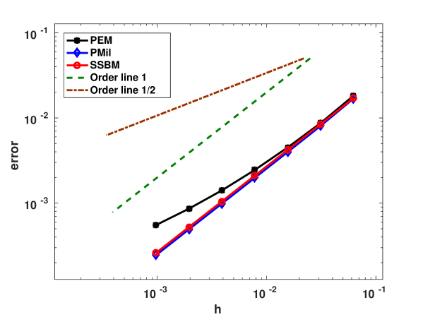
Since there is no explicit expression for the solution of (58) we replace the exact solution by a numerical reference approximation obtained with an extremely small step size $\Delta t=2^{-17}$. For this step-size, the projection onto the $(\Delta t)^{-\alpha}$-ball actually never occurs. The implicit step in the SSBM scheme employs Cardano’s method in order to solve the nonlinear equation exactly. The parameter value was set to $\alpha=\frac{1}{4}$ as prescribed by the results in Section 4 above and in [2]. Figure 1 shows the strong error of convergence for seven different step sizes $h=2^{k}\Delta t,k=7,\dots,13$. The parameter values are $\sigma=0.3$ and $X_{0}=2$, and the coercivity condition (21) always holds.

Figure 1. Strong convergence errors for the approximation of the double well dynamics with parameter $\sigma=0.3$ and $X_{0}=2$.

The strong error is measured at the endpoint $T=1$ by

(60) $$\mathrm{error}=({\mathbb{E}}[|X_{h}(T)-X(T)|^{2}])^{\frac{1}{2}},$$

with a Monte Carlo simulation using $2\cdot 10^{6}$ samples. For this number of samples we estimated the associated confidence intervals. They turned out to be two orders of magnitude smaller than the values of the error itself for all methods and parameters shown. In the scale of Figure 1 they will be hardly visible.

In Figure 1 one observes strong order $\gamma=1$ for the two Milstein-type schemes and strong order $\gamma=\frac{1}{2}$ for the projected Euler-Maruyama method, at least for smaller step-sizes.

Table 2. Strong convergence errors for the approximation of the double well dynamics with parameter $\sigma=0.3$ and $X_{0}=2$.

	PEM			PMil			SSBM
$h$	error	EOC	#	error	EOC	#	error	EOC
$2^{-4}$	0.0183		101912	0.0169		152196	0.0171
$2^{-5}$	0.0087	1.07	0	0.0081	1.07	1	0.0085	1.01
$2^{-6}$	0.0045	0.95	0	0.0040	1.02	0	0.0042	1.01
$2^{-7}$	0.0025	0.88	0	0.0020	1.01	0	0.0021	1.00
$2^{-8}$	0.0014	0.80	0	0.0010	1.00	0	0.0010	1.00
$2^{-9}$	0.0009	0.71	0	0.0005	1.00	0	0.0005	1.00
$2^{-10}$	0.0006	0.64	0	0.0002	1.01	0	0.0003	1.01

Table 2 contains the values of the computed errors and of the corresponding experimental order of convergence defined by

$$\mathrm{EOC}=\frac{\log(\mathrm{error}(h_{i}))-\log(\mathrm{error}(h_{i-1}))}{\log(h_{i})-\log(h_{i-1})},$$

which support the theoretical results. Moreover, as in [2] we are interested in the number of samples for which the trajectories of the PEM method and the PMil scheme leave the sphere of radius $h^{-\alpha}$, i.e. the total number of trajectories we observed the following events

(61) $$\{i=1,\dots,N\colon|X^{\mathrm{PEM}}_{h}(t_{i})|>h^{-\alpha}\}\neq\emptyset,$$

(62) $$\{i=1,\dots,N\colon|X^{\mathrm{PMil}}_{h}(t_{i})|>h^{-\alpha}\}\neq\emptyset,$$

respectively. This information is provided in the fourth and seventh columns of Table 2.

Figure 2. Strong convergence errors for the approximation of the double well dynamics. Parameter values $\sigma=1$ and $X_{0}=2$.

Table 3. Strong convergence errors for the approximation of the double well dynamics. Parameter values $\sigma=0.3$ and $X_{0}=2$.

	PEM			PMil			SSBM
$h$	error	EOC	#	error	EOC	#	error	EOC
$2^{-4}$	0.4611		233635	0.1139		331721	1.2222
$2^{-5}$	0.2525	0.87	877	0.0214	2.41	516	0.1324	3.21
$2^{-6}$	0.1151	1.13	212	0.0118	0.85	168	0.0640	1.05
$2^{-7}$	0.0433	1.41	58	0.0068	0.80	63	0.0389	0.72
$2^{-8}$	0.0161	1.43	21	0.0046	0.58	24	0.0291	0.42
$2^{-9}$	0.0091	0.83	11	0.0037	0.30	9	0.0146	0.99
$2^{-10}$	0.0056	0.69	1	0.0014	1.38	2	0.0081	0.86

(a) The case $\sigma=0.3$.

(b) The case $\sigma=1$.

Figure 3. Single trajectories for the methods PEM, PMil, and SSBM with step size $h=2^{-5}$ versus reference solution (exact) with parameter values $\alpha=\frac{1}{4}$, $X_{0}=2,$ and $T=1$.

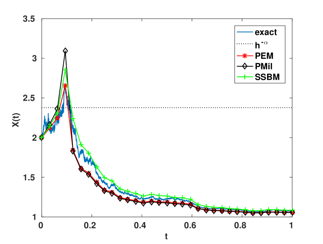
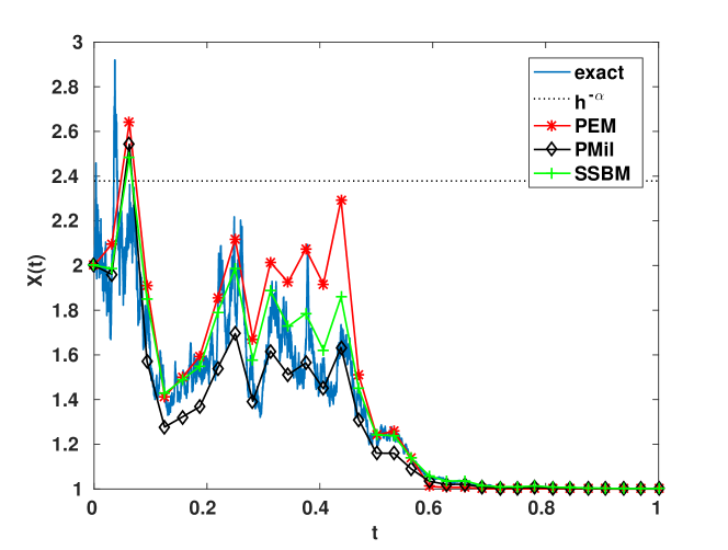
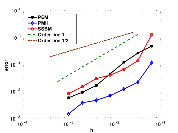
Figure 2 and Table 3 show the results of the strong error of convergence when conditions (4) and (21) in Assumption 2.1 are violated by choosing $\sigma=1$. The estimate of the errors are based on the Monte Carlo simulation with the same number $2\cdot 10^{6}$ of samples as above. And as in the first experiment, confidence intervals are two orders of magnitude smaller than the values themselves. Therefore, we believe that the slightly irregular behavior of the convergence errors is not due to a too small number of samples. Rather we suspect that violation of the convergence conditions influences the expected order of convergence, see the numerical EOC values in Table 3. This effect certainly deserves further investigation. For an illustration we include two runs for parameter values $\sigma=0.3$ and $\sigma=1$ in Figure 3.

Figure 4. CPU times versus $L^{2}$-errors of the PEM, PMil, and SSBM methods for the double well dynamics.

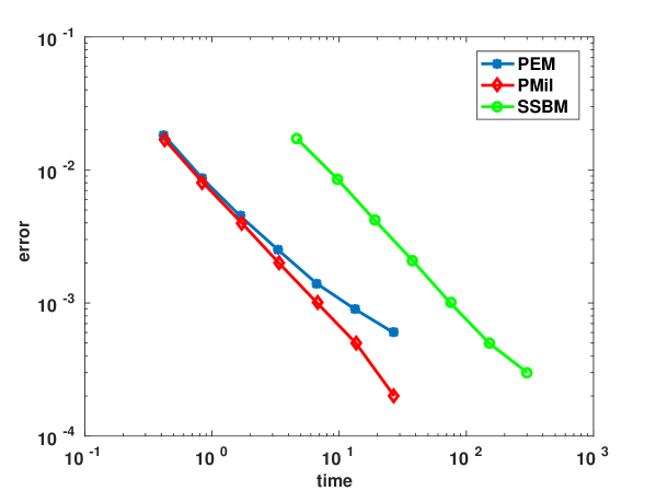
For a fair comparison of computational costs we compiled Figure 4 which shows the $L^{2}$-error versus computing times (measured by tic,toc in MATLAB). One clearly observes that PMil and PEM outperform the split-step backward Milstein method SSBM. Moreover, PMil has a slight advantage over PEM when high accuracy is required.

A stochastic oscillator with commutative noise

(a) Single trajectories of exact solution and PMil scheme.

\psfrag{ax}{$X_{h}(t_{0})$}\psfrag{xb}{$X_{h}(t_{1})$}\psfrag{cx}{$\overline{X}_{h}(t_{2})$}\psfrag{dx}{$X_{h}(t_{2})$}\psfrag{ex}{$X_{h}(t_{3})$}\psfrag{fx}{$\overline{X}_{h}(t_{4})$}\psfrag{gx}{$X_{h}(t_{4})$}\includegraphics[width=346.89731pt]{bild.eps}

(b) Zoom in on the first few steps of the trajectory from (a).

Figure 5. Single trajectory of PMil scheme with step size $h=2^{-4}$ for the stochastic oscillator dynamics. Two projected intermediate steps are indicated by dashed lines. Parameter values $\mu=0.4$, $\sigma_{1}=0.5$, $\sigma_{2}=0.6$, $\theta=1$, $r_{0}=1.97$ and $\varphi_{0}=\frac{\pi}{4}$.

Next, we consider a system in polar coordinates with diagonal noise of the following form

(63) $$\begin{pmatrix}\,\mathrm{d}r(t)\\ \,\mathrm{d}\varphi(t)\end{pmatrix}=\begin{pmatrix}rf_{1}(r^{2})\\ f_{2}(\varphi)\end{pmatrix}\,\mathrm{d}t+\begin{pmatrix}rg_{1}(r^{2})\,\mathrm{d}W^{1}(t)\\ g_{2}(\varphi)\,\mathrm{d}W^{2}(t)\end{pmatrix},$$

where $f_{1},f_{2}$ are smooth functions on $[0,\infty)$ and $g_{1},g_{2}$ are smooth $2\pi$-periodic functions on ${\mathbb{R}}$. We transform to Euclidean coordinates by applying Itō’s formula to $x(r,\varphi)=(r\cos(\varphi),r\sin(\varphi))$,

(64) $$\,\mathrm{d}x(t) =\left[\begin{pmatrix}x_{1}&-x_{2}\\ x_{2}&x_{1}\end{pmatrix}\begin{pmatrix}f_{1}(r^{2})\\ f_{2}(\varphi)\end{pmatrix}-\frac{1}{2}(g_{2}(\varphi))^{2}\begin{pmatrix}x_{1}\\ x_{2}\end{pmatrix}\right]\,\mathrm{d}t$$

$$\quad+g_{1}(r^{2})\begin{pmatrix}x_{1}\\ x_{2}\end{pmatrix}\,\mathrm{d}W^{1}(t)+g_{2}(\varphi)\begin{pmatrix}-x_{2}\\ x_{1}\end{pmatrix}\,\mathrm{d}W^{2}(t).$$

Here we set $r^{2}=x_{1}^{2}+x_{2}^{2}$ and replace $g_{j}(\varphi),j=1,2$ by $g_{j}(\mathrm{arg}(x_{1}+ix_{2}))$ with the argument $\mathrm{arg}(re^{i\varphi})=\varphi$ taken from $(-\pi,\pi]$, for example. In the following computation we treat the special case

(65) $$f_{1}(r^{2})=\mu-r^{2},\quad f_{2}(\varphi)=\theta,\quad g_{1}(r^{2})=\sigma_{1},\quad g_{2}(\varphi)=\sigma_{2}$$

with parameters $\mu,\theta,\sigma_{1},\sigma_{2}\in{\mathbb{R}}$ still to be chosen. This is a generalization of a system studied in [4]. When the parameter $\mu$ varies, this may be considered as a model problem for stochastic Hopf bifurcation (cf. [1, Chap. 9.4.2]).

In this case the system (64) with initial condition $x(0)=(r_{0}\cos(\varphi_{0}),r_{0}\sin(\varphi_{0}))$ can be solved explicitly via (63), since the radial equation is a stochastic Ginzburg Landau equation while the angular equation can be directly integrated. We obtain from [9, Chap. 4.4]

(66) $$r(t) =r_{0}\exp\big{(}(\mu-\frac{\sigma_{1}^{2}}{2})t+\sigma_{1}W^{1}(t)\big{)}$$

$$\qquad\times\Big{(}1+2r_{0}^{2}\int_{0}^{t}\exp\big{(}(2\mu-\sigma_{1}^{2})s+2\sigma_{1}W^{1}(s)\big{)}\,\mathrm{d}s\Big{)}^{-1/2},$$

$$\varphi(t) =\varphi_{0}+\theta t+\sigma_{2}W^{2}(t).$$

Since $g^{1},g^{2}$ are linear and $f$ is cubic with a uniform upper Lipschitz bound, we find that Assumption 2.1 is satisfied with $q=3$. Moreover, the system has commutative noise [9, Chap. 10.3], since

$$g^{1,2}(x)=g^{2,1}(x)=\sigma_{1}\sigma_{2}\begin{pmatrix}-x_{2}\\ x_{1}\end{pmatrix}.$$

As in [9, Chap.10 (3.16)] the double sum in (24), (25) then takes the explicit form

$$\frac{1}{2}\left[\sigma_{1}^{2}((I_{(1)}^{t_{i-1},t_{i}})^{2}-h_{i})-\sigma_{2}^{2}((I_{(2)}^{t_{i-1},t_{i}})^{2}-h_{i})\right]Y+\sigma_{1}\sigma_{2}I_{(1)}^{t_{i-1},t_{i}}I_{(2)}^{t_{i-1},t_{i}}\begin{pmatrix}-Y_{2}\\ Y_{1}\end{pmatrix},$$

where $Y=\overline{X}_{h}^{\mathrm{PMil}}(t_{i})$ and $Y=\overline{X}_{h}^{\mathrm{SSBM}}(t_{i})$, respectively.

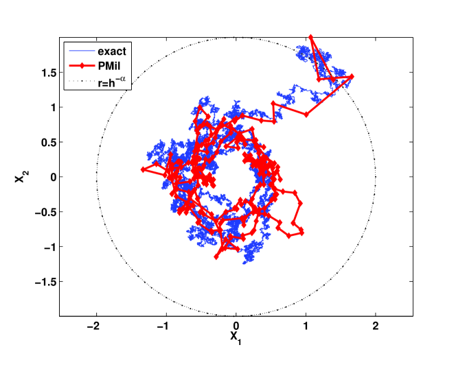
Figure 5 (a) shows the simulation of a single path generated by the exact solution and the projected Milstein method with equidistant step size $h=2^{-4}$ and parameters $\alpha=\frac{1}{4},\mu=0.4,\sigma_{1}=0.5,\sigma_{2}=0.6,\theta=1$, $r_{0}=1.97$, and $\varphi_{0}=\frac{\pi}{4}$. The initial value is $X_{0}=(1.39,1.39)$. Further, we use a highly accurate approximation of the integral in (66) by a Riemann sum with step size $\Delta t=2^{-18}$.

As already mentioned in [2] we are interested in trajectories of the PMil scheme which do not coincide with trajectories generated by the standard Milstein method. Such a case is shown in Figure 5 (a) where the exact trajectory and the PMil-trajectory are displayed. Figure 5 (b) shows a close-up of the projected Milstein scheme near the circle of radius $h^{-\alpha}=2$. In the first and in the third step the trajectory leaves the ball, creating in the next step the intermediate values $\overline{X}_{h}^{\mathrm{PMil}}(t_{2})$ and $\overline{X}_{h}^{\mathrm{PMil}}(t_{4})$, which have been connected by dashed lines to their predecessor and their successor. Obviously, this event occurs more often when the starting point is close to the circle and the values of $\sigma_{1}$ and $\sigma_{2}$ are large.

Figure 6. Strong convergence errors for the approximation of the stochastic oscillator. Parameter values $\mu=0.4$, $\sigma_{1}=0.5$, $\sigma_{2}=0.6$, $\theta=1$, $r_{0}=1.97$, and $\varphi_{0}=\frac{\pi}{4}$.

Table 4. Strong convergence errors for the approximation of the stochastic oscillator. Parameter values $\mu=0.4$, $\sigma_{1}=0.5$, $\sigma_{2}=0.6$, $\theta=1$, $r_{0}=1.97$, and $\varphi_{0}=\frac{\pi}{4}$.

	PEM			PMil			SSBM
$h$	error	EOC	#	error	EOC	#	error	EOC
$2^{-4}$	0.1045		3082	0.07540		4279	0.06741
$2^{-5}$	0.06045	0.79	1	0.03468	1.12	0	0.03445	0.97
$2^{-6}$	0.03838	0.66	0	0.01673	1.05	0	0.01753	0.97
$2^{-7}$	0.02566	0.58	0	0.00823	1.02	0	0.00894	0.97
$2^{-8}$	0.01762	0.54	0	0.00408	1.01	0	0.00464	0.95
$2^{-9}$	0.01226	0.52	0	0.00204	1.01	0	0.00254	0.87
$2^{-10}$	0.00860	0.51	0	0.00102	1.00	0	0.00158	0.69

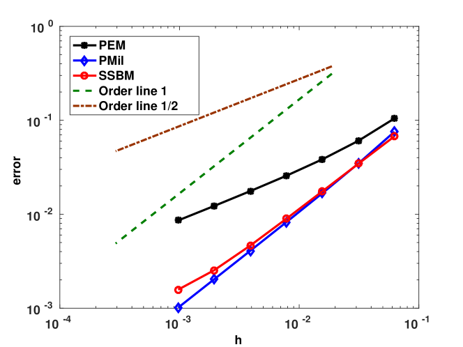
Figure 6 and Table 4 show the estimated strong error of convergence for the PEM scheme, the PMil method, and the SSBM scheme. Nonlinear equations in the scheme SSBM are solved by Newton’s method with three iteration steps. The parameters and the initial value are as in Figure 5.

The estimates of errors, given by (60) at the endpoint $T=1$, with seven different step sizes $h=2^{k}\Delta t,k=8,\dots,14$ are again based on Monte Carlo simulations with $2\cdot 10^{6}$ samples. As above the associated confidence intervals are two orders of magnitude smaller than the estimated errors.

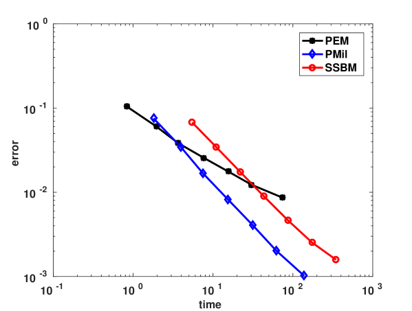
The numerical results in Figure 6 and in Table 4 confirm the theoretical orders of convergence, though with some loss towards smaller step-sizes for the SSBM-method. As in our first example we provide a diagram of error versus computing time in Figure 7. This time PEM has a slight advantage for very rough accuracy, but is worse than PMil and SSBM for higher accuracy. PMil always wins against SSBM.

Figure 7. CPU times versus $L^{2}$-errors of the PEM, PMil, and SSBM methods for the stochastic oscillator.

Acknowledgement

The authors would like to thank Martin Steinborn for bringing several typos to our attention. In addition, the first two authors are grateful for financial support by the DFG-funded CRC 701 ’Spectral Structures and Topological Methods in Mathematics’. Further, this research was carried out by the third named author in the framework of Matheon, project A25, supported by Einstein Foundation Berlin.

References

- [1] L. Arnold. Random dynamical systems. Springer Monographs in Mathematics. Springer-Verlag, Berlin, 1998.
- [2] W.-J. Beyn, E. Isaak, and R. Kruse. Stochastic C-stability and B-consistency of explicit and implicit Euler-type schemes. J. Sci. Comput., 2015. DOI 10.1007/s10915-015-0114-4.
- [3] J. G. Gaines and T. J. Lyons. Random generation of stochastic area integrals. SIAM J. Appl. Math., 54(4):1132–1146, 1994.
- [4] L. Gorini. Theorie und Simulation einer zwei-dimensionalen stochastischen Differentialgleichung. B.Sc. thesis, TU Berlin, 2015.
- [5] D. J. Higham, X. Mao, and A. M. Stuart. Strong convergence of Euler-type methods for nonlinear stochastic differential equations. SIAM J. Numer. Anal., 40(3):1041–1063, 2002.
- [6] D. J. Higham, X. Mao, and L. Szpruch. Convergence, non-negativity and stability of a new Milstein scheme with applications to finance. Discrete Contin. Dyn. Syst. Ser. B, 18(8):2083–2100, 2013.
- [7] M. Hutzenthaler, A. Jentzen, and P. E. Kloeden. Strong and weak divergence in finite time of Euler’s method for stochastic differential equations with non-globally Lipschitz continuous coefficients. Proc. R. Soc. Lond. Ser. A Math. Phys. Eng. Sci., 467(2130):1563–1576, 2011.
- [8] M. Hutzenthaler, A. Jentzen, and P. E. Kloeden. Strong convergence of an explicit numerical method for SDEs with nonglobally Lipschitz continuous coefficients. Ann. Appl. Probab., 22(4):1611–1641, 2012.
- [9] P. E. Kloeden and E. Platen. Numerical Solution of Stochastic Differential Equations. Springer, Berlin, third edition, 1999.
- [10] R. Kruse. Characterization of bistability for stochastic multistep methods. BIT Numerical Mathematics, 52(1):109–140, 2012.
- [11] N. V. Krylov. On Kolmogorov’s equation for finite dimensional diffusions. In Stochastic PDE’s and Kolmogorov equations in infinite dimensions (Cetraro, 1998), pages 1–63. Lecture Notes in Math., vol. 1715, Springer, Berlin, 1999.
- [12] C. Kumar and S. Sabanis. On tamed Milstein schemes of SDEs driven by Lévy noise. Preprint, arXiv:1407.5347v2, 2015.
- [13] C. Kumar and S. Sabanis. On Milstein approximations with varying coefficients: the case of super-linear diffusion coefficients. Preprint, arXiv:1601.02695, 2016.
- [14] X. Mao. Stochastic differential equations and their applications. Horwood Publishing Series in Mathematics & Applications. Horwood Publishing Limited, Chichester, 1997.
- [15] G. N. Milstein. Approximate integration of stochastic differential equations. Teor. Verojatnost. i Primenen., 19:583–588, 1974. in Russian.
- [16] G. N. Milstein. Approximate integration of stochastic differential equations. Theory Probab. Appl., 19(3):557–562, 1975. translated by K. Durr.
- [17] G. N. Milstein. Numerical integration of stochastic differential equations, volume 313 of Mathematics and its Applications. Kluwer Academic Publishers Group, Dordrecht, 1995. Translated and revised from the 1988 Russian original.
- [18] G. N. Milstein and M. V. Tretyakov. Stochastic Numerics for Mathematical Physics. Scientific Computation. Springer-Verlag, Berlin, 2004.
- [19] J. M. Ortega and W. C. Rheinboldt. Iterative solution of nonlinear equations in several variables, volume 30 of Classics in Applied Mathematics. Society for Industrial and Applied Mathematics (SIAM), Philadelphia, PA, 2000. Reprint of the 1970 original.
- [20] C. Prévôt and M. Röckner. A Concise Course on Stochastic Partial Differential Equations, volume 1905 of Lecture Notes in Mathematics. Springer, Berlin, 2007.
- [21] T. Rydén and M. Wiktorsson. On the simulation of iterated Itô integrals. Stochastic Process. Appl., 91(1):151–168, 2001.
- [22] A. M. Stuart and A. R. Humphries. Dynamical Systems and Numerical Analysis, volume 2 of Cambridge Monographs on Applied and Computational Mathematics. Cambridge University Press, Cambridge, 1996.
- [23] X. Wang and S. Gan. The tamed Milstein method for commutative stochastic differential equations with non-globally Lipschitz continuous coefficients. J. Difference Equ. Appl., 19(3):466–490, 2013.
- [24] M. Wiktorsson. Joint characteristic function and simultaneous simulation of iterated Itô integrals for multiple independent Brownian motions. Ann. Appl. Probab., 11(2):470–487, 2001.
- [25] Z. Zhang. New explicit balanced schemes for SDEs with locally Lipschitz coefficients. Preprint, arXiv:1402.3708, 2014.