Truncated Hilbert space approach to the 2d $\phi^{4}$ theory

Abstract

We apply the massive analogue of the truncated conformal space approach to study the two dimensional $\phi^{4}$ theory in finite volume. We focus on the broken phase and determine the finite size spectrum of the model numerically. We interpret the results in terms of the Bethe-Yang spectrum, from which we extract the infinite volume masses and scattering matrices for various couplings. We compare these results against semiclassical analysis and perturbation theory. We also analyze the critical point of the model and confirm that it is in the Ising universality class.

1 Introduction

Interactive quantum field theories (QFT) cannot be solved exactly. There are some exceptions including two dimensional integrable QFTs, which can be investigated by the bootstrap method, but these theories are very special, as the scattering matrix is factorized and there is no particle production or decay. To study more realistic QFTs, one has to rely on alternative approximative methods such as perturbation theory, variational methods, lattice discretizations or the truncated conformal space approach (TCSA) just to mention a few.

The truncated conformal space approach was originally developed by Yurov and Zamolodchikov to study the relevant perturbation of the Lee-Yang conformal field theory [1]. The idea of the method is to put the system in a finite volume, which makes the spectrum discrete, then one can truncate the Hilbert space by keeping states below some energy cut and diagonalize the truncated Hamiltonian numerically to get an approximate spectrum as the function of the volume. This is basically the usual variational method of quantum mechanics with the unperturbed energy levels as basis states and the obtained results are not perturbative.

The TCSA method has been extended to analyze the perturbation of other conformal field theories [2, 3, 4], too. The advantage of the method is that it can be applied for non-integrable perturbations [5]. Indeed it has been successfully applied to describe such phenomena as phase transitions, decay rates, form factors or boundary entropies [5, 6, 7, 8]. It also has a natural extension for models with boundaries and with a defect [9, 10]. Recently the method has been extended even to higher dimensional theories [11].

The simplest non-integrable interacting quantum field theory is probably the two dimensional $\phi^{4}$ theory. The TCSA method was used in [12] to study the spectrum by compactifying the zero mode of the field. This approach gives a good result for small couplings. Alternatively, in [13, 14] the authors used the finite volume massive basis to build up the truncated Hilbert space and analyzed both the unbroken and the broken phases of the model for a wide range of couplings. There special emphasis was put on developing the method and on analyzing carefully the convergence properties in eliminating the truncation. The authors also searched for the critical point, beyond which the parity symmetry is broken and checked Chang duality, by which one can realize the same system with two different parameter sets, which are related to each other in a strong-weak fashion. The truncation dependence of the spectrum was further analyzed in [15]. The aim of our paper is to use the same truncation of the finite volume massive basis for the broken phase and obtain results for a wide range of couplings similarly to [13, 14]. We focus on the volume dependence of the spectrum and try to extract the infinite volume parameters from finite size effects. This analysis requires precise data, which we achieved, first, by implementing an efficient diagonalizing routine for large sparse matrices, and second, by an extrapolation in the truncation level. We compare the extrapolated finite size spectrum with semiclasssical results, perturbative results and also with the Bethe-Yang (BY) spectrum. This BY spectrum incorporates the leading finite size corrections based on the infinite volume masses and scattering data and enables one to determine these infinite volume characteristics at moderate volumes when the truncation errors can be controlled.

The paper is organized as follows:

In section 2 we review the classical and semiclassical results. Section 3 contains the definition of the quantum model. In section 4 we explain our truncated Hilbert space method. Theoretical predictions are summarized in section 5, while numerical results are presented in section 6 and compared to both the semiclassical, the perturbative and to the Bethe-Yang spectrum. From this comparison we extract the infinite volume mass spectrum and scattering phases. We also analyze the spectrum near the critical point. We close the paper with conclusions in section 7. Appendix A explains volume dependent normal ordering and its relation to the ground-state energy. Appendix B introduces the parametrization of the scattering matrix from unitarity relations, while Appendix C explains the numerical implementations.

2 Classical, semiclassical and perturbative results

In this section we recall the available results for our theory

$$\mathcal{L=}\frac{1}{2}\left(\partial_{t}\phi\right)^{2}-\frac{1}{2}\left(\partial_{x}\phi\right)^{2}+\frac{1}{2}m^{2}\phi^{2}-\frac{\lambda}{4!}\phi^{4}$$ (1)

We follow [12], but see also [16, 17] for more details. Sometimes we simplify formulas by introducing $q$ as $\lambda=6q^{2}$. We take $\hbar=c=1$. As in two dimensions the scalar field is dimensionless, both $m$ and $q$ have dimension of energy, i.e. $1$. The parameter $m$ can be chosen to determine the mass scale and then the physics depends on the dimensionless ratio: $\frac{m}{q}$. Observe that the coefficient of $\phi^{2}$ has a “wrong” sign, such that we analyze the theory when the $\mathbb{Z}_{2}$ parity symmetry will be spontanously broken.

2.1 Classical analysis

The potential has two minima at $\pm\frac{m}{q}$ and its expansions around the minima reads as

$$V\left(\pm\frac{m}{q}+\eta\right)=-\frac{m^{4}}{4q^{2}}+m^{2}\eta^{2}\pm mq\eta^{3}+\frac{q^{2}}{4}\eta^{4}\equiv V_{0}+\frac{m_{0}^{2}}{2}\eta^{2}+\dots$$ (2)

The mass of the small fluctuations is $m_{0}=\sqrt{2}m$ and the minimum of the potential is $V_{0}=-\frac{m^{4}}{4q^{2}}$. The two static solutions, called the kink and the antikink, interpolate between the vacua as

$$\phi_{\pm}=\pm\frac{m}{q}\tanh\left(\frac{mx}{\sqrt{2}}\right)$$ (3)

and have masses

$$M_{0}=\frac{2\sqrt{2}m^{3}}{3q^{2}}=\frac{m_{0}}{g}\quad;\qquad g=\frac{3q^{2}}{2m^{2}}=\frac{\lambda}{4m^{2}}$$ (4)

The breather-like bound state of the kink and the antikink is not a stable solution as it radiates very slowly [18].

2.2 Semiclassical considerations

We can quantize the theory semiclassically. For this normal ordering is needed, which has to be defined wrt. a free theory. We recall for later reference that in the calculations [16, 17] the reference theory was chosen to be the infinite volume free massive theory describing the fluctuations around any of the minima with mass $m_{0}$. The relevant quantities at the quantum level are the masses and the scattering matrix.

The semiclassical corrections to the kink masses read as

$$M=M_{0}-m_{0}c+\mathcal{O}\left(q^{2}\right)\quad;\qquad c=\frac{3}{2\pi}-\frac{1}{4\sqrt{3}}$$ (5)

where, as we pointed out, the parameters $m,q$ are understood as the coefficients of the normal ordered perturbations wrt. $m_{0}$.

The breathers can be considered as kink-antikink bound states with masses [19]

$$m_{n}=2M\sin\Bigl{(}n\frac{\zeta}{2}\Bigr{)}$$ (6)

where

$$\zeta=\frac{g}{1-gc}=\frac{\frac{3q^{2}}{2m^{2}}}{1-\frac{3q^{2}}{2m^{2}}\left(\frac{3}{2\pi}-\frac{1}{4\sqrt{3}}\right)}$$ (7)

Although classically there is no stable breather solution due to the radiation into the small fluctuations of the field, at the quantum level the small fluctuations are indentified with the breather itself thus can be stable. Higher breathers are bound states of the lightest one

$$m_{n}=m_{0}n\left(1-\frac{3q^{4}}{32m^{4}}n^{2}+\dots\right)=m_{0}n\left(1-\frac{g^{2}}{24}n^{2}+\dots\right)$$ (8)

The existence of the $n^{th}$ bound state requires the scattering pole $n\zeta$ to be in the physical strip: $n\zeta<\pi$, i.e. $\zeta<\frac{\pi}{n}$. The stability against the lighest particle further requires that $m_{n}<2m_{1}$, which is always satisfied for $m_{2}$ but never for $m_{3}$ and for the higher ones. It was conjectured in [19] that this picture survives at the quantum level in the sense that we cannot have more than two breathers. Let us anticipate that in the deep quantum domain even the first breather is unstable against decaying into a kink and antikink pair.

The scattering matrix for the lightest breather satisfies unitarity and crossing symmetry below the two-particle threshold

$$S(\theta)=S(-\theta)^{-1}=S(i\pi-\theta)$$ (9)

Here we introduced the rapidity variable, see Appendix B for details. The simplest non-trivial solution of (9) is

$$S(\theta,i\kappa)=\frac{\sinh\theta+i\sin\kappa}{\sinh\theta-i\sin\kappa}$$ (10)

It implies a bound state with mass $m_{2}=2m_{1}\cos\frac{\kappa}{2}$. Comparing this to the semiclassical mass formula 8, we conclude that $\kappa=\zeta$.

From the analysis of the small fluctuations over the kink solution the classical limit of the breather-kink scattering matrix can also be extracted [16]:

$$S_{bk}(\theta)=S\left(\theta,i\frac{\pi}{2}\right)S\left(\theta,i\frac{\pi}{6}\right)$$ (11)

The pole at $\theta=i\pi/2$ is related to the translational mode, while the pole at $\theta=i\pi/6$ signals an excited kink state with mass

$$M^{*}=M+m_{0}\frac{\sqrt{3}}{2}$$ (12)

2.3 Related integrable models and perturbative results

There are two integrable models, which are related to our theory. The sinh-Gordon theory is defined by the Lagrangian

$$\mathcal{L}=\frac{1}{2}\left(\partial_{t}\phi\right)^{2}-\frac{1}{2}\left(\partial_{x}\phi\right)^{2}-\frac{m^{2}}{b^{2}}(\cosh b\phi-1)$$ (13)

It contains only one type of particle with scattering matrix

$$S(\theta)=S(\theta,-i\pi p)\quad;\qquad p=\frac{b^{2}}{8\pi+b^{2}}=\frac{b^{2}}{8\pi}+\dots$$ (14)

The sine-Gordon theory can be obtained by an analytical continuation $b\to i\beta$, which admits kink and anti-kink solutions, too.

The other interesting theory is the Bullough-Dodd theory

$$\mathcal{L}=\frac{1}{2}\left(\partial_{t}\phi\right)^{2}-\frac{1}{2}\left(\partial_{x}\phi\right)^{2}-\frac{m^{2}}{6g^{2}}\left(2e^{g\phi}+e^{-2g\phi}\right)$$ (15)

Its scattering matrix has the form [20]

$$S(\theta)=S\left(\theta,i\frac{\pi}{3}\right)S\left(\theta,i\frac{\pi B}{3}\right)S\left(\theta,i\frac{\pi(2-B)}{3}\right)\,\quad;\qquad B=\frac{g^{2}}{2\pi}\frac{1}{1+\frac{g^{2}}{4\pi}}=\frac{g^{2}}{2\pi}+\dots$$ (16)

Combining the perturbative expansions of the two models one can extract the leading order perturbative S-matrix of our model:

$$S(\theta)=1+2ig\frac{(2+\cosh 2\theta)}{\sinh 3\theta}+\dots$$ (17)

Direct perturbative calculation for the mass correction gives [14]:

$$m_{pert}^{2}(g)-m_{0}^{2}=m_{0}^{2}\left(-\frac{g}{2\sqrt{3}}-0.0317182g^{2}\right)$$ (18)

We would like to compare all of the results of this section against the finite size spectrum we obtain from our truncated Hilbert space approach.

3 Quantum theory

At the quantum level we analyze the spectrum of the Hamiltonian in a finite volume $L$:

$$H=\int_{0}^{L}\mathcal{H}\,dx\quad;\qquad\mathcal{H}=\frac{1}{2}\left(\partial_{t}\phi\right)^{2}+\frac{1}{2}\left(\partial_{x}\phi\right)^{2}-\frac{1}{2}m^{2}\phi^{2}+\frac{\lambda}{4!}\phi^{4}$$ (19)

where $\phi(x)=\pm\phi(x+L)$, i.e. we consider both periodic ($+$) and antiperiodic ($-$) boundary conditions in order to accommodate one-particle kink states.

As operators are multiplied in the same position we need to regulate them by normal ordering. Normal ordering is performed with respect to some prescribed mass scale $\mu$ and volume $L$, thus the Hamiltonian density takes the form:

$$\mathcal{H}=\mathcal{H}_{0}^{\mu,L}+g_{2}(\mu,L):\!\phi^{2}\!:_{\mu,L}+g_{4}(\mu,L):\!\phi^{4}\!:_{\mu,L}+g_{0}(\mu,L)$$ (20)

Here the field is expressed in terms of creation-annihilation operators as

$$\phi(x,t)=\sum_{n}\frac{1}{\sqrt{2\omega_{n}L}}\left(a_{n}e^{-i\omega_{n}t+ik_{n}x}+a_{n}^{+}e^{i\omega_{n}t-ik_{n}x}\right)$$ (21)

where

$$[a_{n},a_{m}]=[a_{n}^{+},a_{m}^{+}]=0\quad;\qquad[a_{n},a_{m}^{+}]=\delta_{n,m}$$ (22)

and

$$\omega_{n}=\sqrt{\mu^{2}+k_{n}^{2}}\quad;\qquad k_{n}=\frac{2\pi}{L}n$$ (23)

The index $n$ takes integer values for periodic, while half-integer values for antiperiodic boundary conditions. Normal ordering, denoted above by $::_{\mu,L}$, is understood that all creation operators $a_{n}^{+}$ are on the left of the annihilation operators $a_{n}$. The vacuum is chosen to be annihilated by all $a_{n}$. The free Hamiltonian is

$$H_{0}^{\mu,L}=\frac{1}{2}\int_{0}^{L}:\left(\partial_{t}\phi\right)^{2}+\left(\partial_{x}\phi\right)^{2}+\mu^{2}\phi^{2}:_{\mu,L}+E_{0}^{\pm}(\mu,L)=\sum_{n}\omega_{n}\,a_{n}^{+}a_{n}+E_{0}^{\pm}(\mu,L)$$ (24)

where the renormalized ground-state energy is chosen to be

$$E_{0}^{\pm}(\mu,L)=\mu\int_{-\infty}^{\infty}\frac{d\theta}{2\pi}\cosh\theta\log\left(1\mp e^{-mL\cosh\theta}\right)$$ (25)

for periodic/antiperiodic boundary conditions. Since both the ground-state energy and the ground-state energy density is infinite for the non-renormalized Hamiltonian, we have to introduce proper renormalization. In Appendix A, we show how $E_{0}^{\pm}(\mu,L)$ appears from comparing different renormalization schemes. In our scheme the vacuum energy density is normalized to zero and the ground-state energy is chosen to vanish for infinite volume.

To relate (20) to another normal ordering at scale $\mu^{\prime}$ and volume $L^{\prime}$, we recall that [12, 13]

$$:\!\phi^{2}\!:_{\mu^{\prime},L^{\prime}}=:\!\phi^{2}\!:_{\mu,L}+\Delta Z\quad;\quad\Delta Z=Z(\mu,L)-Z(\mu^{\prime},L^{\prime})$$ (26)

where

$$Z(\mu,L)=\sum_{|n|<N}\frac{1}{2\omega_{n}L}$$ (27)

$Z(\mu,L)$ itself is only meaningful with a UV cutoff $N$, but in the difference, $\Delta Z$, the limit $N\rightarrow\infty$ can be taken. Similarly

$$:\!\phi^{4}\!:_{\mu^{\prime},L^{\prime}}=:\!\phi^{4}\!:_{\mu,L}+6\Delta Z:\!\phi^{2}\!:_{\mu,L}+3(\Delta Z)^{2}$$ (28)

As we already mentioned, the scheme in which the semiclassical calculations were done is defined by normal ordering at $L^{\prime}=\infty$ and $\mu^{\prime}=m_{0}$. The parameters are chosen there as

$$g_{2}\left(m_{0},\infty\right)=-\frac{3}{2}m^{2}\quad;\qquad g_{4}\left(m_{0},\infty\right)=\frac{q^{2}}{4}\quad;\qquad g_{0}\left(m_{0},\infty\right)=0$$ (29)

To relate this scheme to the one with mass $m$ and $L=\infty$, we calculate

$$Z(m,\infty)-Z(m_{0},\infty)=\frac{1}{2\pi}\int_{0}^{\infty}\left(\frac{1}{\sqrt{1+k^{2}}}-\frac{1}{\sqrt{2+k^{2}}}\right)dk=\frac{\ln 2}{4\pi}$$ (30)

such that the coefficients of the same physical system in this scheme are

$$g_{2}(m,\infty)=-m^{2}+\frac{3q^{2}\ln 2}{8\pi}=m^{2}\left(g\frac{\ln 2}{4\pi}-1\right)\quad;\qquad g_{4}(m,\infty)=\frac{q^{2}}{4}$$ (31)

and

$$g_{0}(m,\infty)=-\frac{3}{2}m^{2}\frac{\ln 2}{4\pi}+\frac{3}{4}q^{2}\left(\frac{\ln 2}{4\pi}\right)^{2}$$ (32)

As we work in the finite volume scheme we introduce [13]:

$$z(mL)=Z(m,L)-Z(m,\infty)$$ (33)

For periodic boundary condition we have

$$z^{+}(mL)=\int_{0}^{\infty}\frac{d\theta}{\pi}\left(e^{mL\cosh\theta}-1\right)^{-1}$$ (34)

while for antiperiodic boundary condition we found

$$z^{-}(mL)=2z^{+}(2mL)-z^{+}(mL)$$ (35)

The coefficient at volume $L$ of our theory are given by:

$$g_{2}(m,L) = m^{2}\tilde{g}_{2}(mL)\quad;\qquad\tilde{g}_{2}(mL)=\left[g\,\tilde{z}(mL)-1\right]\quad;\quad\tilde{z}(x)=z^{\pm}(x)+\frac{\ln 2}{4\pi}$$

$$g_{4}(m,L) = m^{2}\tilde{g}_{4}\quad;\qquad\tilde{g}_{4}=\frac{g}{6}$$ (36)

The correction to the vacuum energy density due to normal ordering is

$$g_{0}(m,L)=m^{2}\tilde{g}_{0}(m,L)\quad;\qquad\tilde{g}_{0}(m,L)=-z^{\pm}(mL)-\frac{3}{2}\frac{\ln 2}{4\pi}+\frac{g}{2}\tilde{z}(mL)^{2}$$ (37)

Since $z^{\pm}(L)$ is exponentially small, it can be often neglected.

It is tempting to introduce the normal ordering at $\mu=0$ and $L=\infty$, as then the scale would not appear as a dimensionful parameter [12]. Choosing $\mu=0$ implies, however, that $Z(0,\infty)-Z(m_{0},\infty)$ is IR divergent, which can be regulated by an IR cutoff $a,$

$$Z(0,\infty)=\frac{1}{2\pi}\int_{a}^{\Lambda}\frac{dk}{k}=\frac{1}{2\pi}\ln\left(\frac{\Lambda}{a}\right)$$ (38)

but then the theory will depend on the regulator $a$. Naively we could just use $Z(0,L)$ (conformal scheme) instead of introducing $Z(0,\infty)$ but we should keep in mind that $L\to\infty$ is not a safe limit as it basically puts $a$ to zero. As a result, the mass of the breather will diverge logarithmically in the $L\to\infty$ limit in this conformal scheme.

4 Truncated Hilbert space approach

In this section we explain how we diagonalize the finite volume Hamiltonian. For numerical investigations we introduce dimensionless quantities

$$\frac{H}{m}=h\quad;\qquad mL=l\quad;\quad\omega_{n}=m\tilde{\omega}_{n}=m\sqrt{1+\frac{4\pi^{2}n^{2}}{l^{2}}}$$ (39)

such that the dimensionless Hamiltonian can be written as

$$\tilde{h}=\tilde{h}_{0}+\int_{0}^{L}mdx\left[\tilde{g}_{2}(l):\!\phi^{2}\!:+\tilde{g}_{4}:\!\phi^{4}\!:+\tilde{g}_{0}(l)\right]$$ (40)

where

$$\tilde{h}_{0}=\sum_{n}\tilde{\omega}_{n}(l)a_{n}^{+}a_{n}+\tilde{e}_{0}^{\pm}(l)$$ (41)

and $\tilde{e}_{0}^{\pm}(l)=E_{0}^{\pm}(mL)/m$. From now on all normal orderings are evaluated at scale $m$ and volume $L$, unless otherwise indicated.

Technically we use the Hilbert space built up by the oscillators of the free Hamiltonian in volume $L$ and diagonalize $h$ at a certain truncation level. Clearly we have two dimensionless parameters: the dimensionless volume $l$ and the quartic coupling parameter $g$. The dimensionful mass $m$ sets purely the energy scale.

4.1 Mini Hilbert space approach

For periodic boundary condition we found it useful to adapt the “mini-superspace” approach. This is the method which was used many times in analyzing the Liouville theory and deals with the zero mode of the field separately [21, 22, 23]. The same approach was used also in [14] to handle the zero mode. Here we also found that the IR mode generated by $a_{0}$ and $a_{0}^{+}$ plays a very special role in forming the low lying states in the spectrum. We thus decompose the elementary field as

$$\phi(x,0)=\tilde{\phi}(x,0)+\phi_{0}\quad;\qquad\phi_{0}=\frac{1}{\sqrt{2l}}\left(a_{0}+a_{0}^{+}\right)$$ (42)

and analyze the mode $\phi_{0}$ first. It has the Hamiltonian

$$h^{\textrm{mini}}=\tilde{\omega}_{0}\,a_{0}^{+}a_{0}+\frac{1}{2}\tilde{g}_{2}(l):\!\left(a_{0}+a_{0}^{+}\right)^{2}\!:+\frac{1}{4l}\tilde{g}_{4}:\!\left(a_{0}+a_{0}^{+}\right)^{4}\!:$$ (43)

which we diagonalize seperately and use its eigenvalues and eigenvectors to calculate the matrix elements of the full Hamiltonian:

$$h=h^{\textrm{mini}}+\tilde{h}_{0}+\int_{0}^{L}mdx\left[\tilde{g}_{0}(l)+\tilde{g}_{2}(l):\!\tilde{\phi}^{2}:+\tilde{g}_{4}\left(:\!\tilde{\phi}^{4}\!:+4:\!\tilde{\phi}^{3}\!:\phi_{0}+6:\!\tilde{\phi}^{2}\!:\phi_{0}^{2}\right)\right]$$ (44)

where $\tilde{h}_{0}=h_{0}-h_{0}^{\mathrm{mini}}$ and $h_{0}^{\mathrm{mini}}=\tilde{\omega}_{0}\,a_{0}^{+}a_{0}$ denotes the harmonic oscillator Hamiltonian of the zero mode.

4.2 Technical implementations

For periodic boundary condition we split the Hilbert space to the mini-Hilbert space containing the zero mode of the field and to the rest:

$$\mathcal{H}=\mathcal{H}^{\mathrm{mini}}\otimes\tilde{\mathcal{H}}$$ (45)

The mini-Hilbert space $\mathcal{H}^{\mathrm{mini}}$ is generated from the vacuum by acting with $a_{0}^{+}$, while $\tilde{\mathcal{H}}$ by acting with all other creation operators $a_{n\neq 0}^{+}$. Technically we determine the spectrum of $h^{\mathrm{mini}}$ first. For this we choose $2000$ eigenstates of $h_{0}^{\mathrm{mini}}$ and diagonalize $h^{\mathrm{mini}}$ on these states. We found it enough to use only the first $6$ states to build up the relevant product basis for (45).

For antiperiodic boundary condition we do not have the analogue of the mini Hilbert space, so we diagonalize the Hamiltonian on the full truncated Hilbert space.

We want to keep the dimension of the truncated space for each volume. Since by changing the volume the free energy levels are changing, too, we decided to generate the basis for the Hilbert space at $mL=1$. At such a small volume the spectrum is close to the conformal spectrum and the energy can be approximately measured in units of $\frac{2\pi}{mL}$. Consequently, the mode $(a_{n}^{+})^{j_{n}}$ contributes to this “conformal energy” as $j_{n}|n|.$ We introduce integer cuts in this unit, which we increase two by two (one by one in the antiperiodic sector), usually between $14$ and $26$. With each cut we keep the same oscillator content for any dimensionless volume, which typically takes integer values up to $l=30$.

There are conserved charges in the theory, which help to decrease the dimension of the Hamiltonian below the energy cut in each sectors. Momentum is a conserved quantity and we focus through the whole paper on the zero-momentum sector. Field parity $\phi\leftrightarrow-\phi$ is also a symmetry of the full theory. As a consequence we can diagonalize the Hamiltonian separately on the even and odd particle number sectors. Additionally, there is also space parity $x\leftrightarrow-x$, but in this paper we will not exploit this symmetry.

5 Description of the spectrum

According to Lüscher, the finite size spectrum of a quantum field theory can be described in terms of the infinite volume data [24, 25]. These data consist of the masses of the excitations, their dispersion relation and the various scattering matrices. The leading finite size correction comes from momentum quantization, which is described by Bethe-Yang type equations and expresses the periodicity of the multiparticle wave function[25]. These corrections are polynomial in the inverse power of the volume. There are exponentially small corrections, too, and they are related to vacuum polarization effects, or some other words, virtual particles [24, 26].

5.1 Infinite volume data

In infinite volume, the theory is parametrized by the masses of the excitations and their scattering matrices. We use unitarity and consistency with a generalized bootstrap idea to restrict the form of the scattering matrices and masses. The bootstrap idea states that the scattering matrix of the bound state is the product of the scattering matrices of it constituents. It is definitely satisfied in integrable theories and we expect that it is also satisfied for nonintegrable theories below the inelastic threshold.

Let us start with the breathers. According to the semiclassical analysis, we can have at most two breathers. Let us denote the lighter one by $B_{1}$ and its mass by $m_{1}$, while the heavier is denoted by $B_{2}$, whose mass is $m_{2}$. As we are in a relativistic theory their dispersion relation is

$$E_{i}(p)=\sqrt{m_{i}^{2}+p^{2}}$$ (46)

This motivates to introduce the rapidity parameter:

$$E_{i}(\theta)=m_{i}\cosh\theta\quad;\qquad p_{i}(\theta)=m_{i}\sinh\theta$$ (47)

Lorentz transformation simply shifts the rapidity and, as a consequence, the scattering matrix depends only on their differences. Since $B_{2}$ is the bound state of two $B_{1}$s, the $B_{1}B_{1}\to B_{1}B_{1}$ two-particle scattering matrix, which we denote simply by $S_{11}(\theta)$, must have a pole whenever $B_{2}$ is in the spectrum. In Appendix B we derive a parametrization of the scattering matrix with the existence of the required pole from unitarity:

$$S_{11}(\theta)=S(\theta,i\alpha)S_{11}^{\mathrm{exp}}(\theta)$$ (48)

where

$$S_{11}^{\mathrm{exp}}(\theta)=\exp\left\{-\int_{\theta_{t}}^{\infty}\frac{d\theta^{\prime}}{2\pi i}\rho_{11}(\theta^{\prime})\log S(\theta^{\prime},\theta)\right\}\quad;\qquad S(\theta,x)=\frac{\sinh\theta+\sinh x}{\sinh\theta-\sinh x}$$ (49)

and the position of the pole $i\alpha$ and the density $\rho_{11}(\theta)$ is an unknown function of the dimensionless parameter $g$. The threshold rapidity $\theta_{t}$ corresponds to the kinematical point where the $B_{1}B_{1}\to B_{1}B_{2}$ or the $B_{1}B_{1}\rightarrow\overline{K}K$ channels opens. Semiclassically, for small $g$, according to 7, the parameter $\alpha$ starts as

$$\alpha=g+\dots$$ (50)

In the analysis we will assume that $\theta_{t}$ is large and the exponential piece can be neglected. It would be very interesting, although not easy, to measure this piece and compare it to other scattering matrix elements.

Since the scattering matrix has a pole at $i\alpha$:

$$S_{11}(\theta)=i\frac{\Gamma^{2}}{\theta-i\alpha}\quad;\qquad\Gamma=\sqrt{2\tan\alpha}$$ (51)

the mass of the bound state $m_{2}$ can be expressed as

$$m_{2}=2m_{1}\cos\frac{\alpha}{2}$$ (52)

Below the $\theta_{t}$ threshold the scattering matrix behaves as if it were in an integrable theory. As a consequence one can try to use bootstrap to calculate the scattering matrix of $B_{2}$ on $B_{1}$

$$S_{21}(\theta)=S_{11}\left(\theta-i\frac{\alpha}{2}\right)S_{11}\left(\theta+i\frac{\alpha}{2}\right)\tilde{S}_{21}^{\mathrm{exp}}(\theta)=S\left(\theta,i\frac{\alpha}{2}\right)S\left(\theta,i\frac{3\alpha}{2}\right)\tilde{S}_{21}^{\mathrm{exp}}(\theta)$$ (53)

however, this scattering could be intercepted by the $B_{2}B_{1}\to B_{1}B_{1}$ process, which is taken into account partially by $\tilde{S}_{21}^{\mathrm{exp}}(\theta)$. Additionally the appearing pole at $i\frac{3\alpha}{2}$ should correspond to a resonance, since $B_{3}$ is not a stable particle, i.e. it should not lie on the imaginary line. All together the correct parametrization possibly is

$$S_{21}(\theta)=S\left(\theta,i\frac{\alpha}{2}\right)S_{21}^{\mathrm{exp}}(\theta)$$ (54)

Let us focus on the kink and the antikink now. The $\mathbb{Z}_{2}$ symmetry implies that these particles are degenerate in their mass, what we denote by $M$. Interestingly the kink–antikink scattering matrix is also diagonal and satisfies crossing symmetry and unitarity below the threshold [19]:

$$S_{k\bar{k}}(\theta)=S_{\bar{k}k}(i\pi-\theta)=S_{\bar{k}k}(-\theta)^{-1}=S_{\bar{k}k}(\theta)$$ (55)

where in the last line we used charge conjugation symmetry. A kink–antikink pair can fuse either to $B_{1}$ or to $B_{2}$. The corresponding angles are $\beta_{1}$ and $\beta_{2}$, such that the masses are $m_{n}=2M\cos\frac{\beta_{n}}{2}$. The fusion process is shown on Figure 1. This further implies that

$$S_{k\bar{k}}(\theta)=-S\left(\theta,i\beta_{1}\right)S\left(\theta,i\beta_{2}\right)S_{k\bar{k}}^{\mathrm{exp}}(\theta)$$ (56)

where we included $S_{k\bar{k}}^{\mathrm{exp}}(\theta)$ for later consistency, which has a similar form as (48). Here it is assumed that we are in the domain where the kink is the lightest particle. Note that kinematically it happens in a different domain of the coupling $g$ , where we can trust in (48) without the exponential piece.

Figure 1: The kink–anti-kink $B_{1}$ fusion process, together with the corresponding pole in the kink $B_{1}$ scattering process.

The kink-$B_{1}$ sector has a topological charge which separates it from the neutral sector. Thus, even for $m_{1}<M$, the scattering matrix $S_{k1}$ also satisfies unitarity and crossing symmetry below the kink-$B_{2}$ threshold

$$S_{k1}(\theta)=S_{1\bar{k}}(i\pi-\theta)=S_{1k}(-\theta)^{-1}=S_{1k}(\theta)=S_{1\bar{k}}(\theta)$$ (57)

where again we used parity and charge conjugation symmetry. Due to the kink–anti-kink fusion process this scattering matrix must have a pole at $i\frac{\beta_{1}}{2}$ as demonstrated on Figure 1. Taking into account that in the classical limit (11) we have a pole at $\theta=i\pi/6$ , which could get quantum correction $\gamma$, we arrive at the parametrization

$$S_{k1}(\theta)=-S\left(\theta,i\frac{\beta_{1}}{2}\right)S\left(\theta,i\left(\frac{\pi}{6}+\gamma\right)\right)S_{k1}^{\mathrm{exp}}(\theta)$$ (58)

Demanding that fusing a kink with an antikink we obtain the breather-breather S-matrix

$$S_{k1}\left(\theta+i\frac{\beta_{1}}{2}\right)S_{\bar{k}1}\left(\theta-i\frac{\beta_{1}}{2}\right)=S_{11}(\theta)$$ (59)

the existence of the factor $S(\theta,i\alpha)$implies that $\beta_{1}=\pi-\alpha$ (for $\alpha<\frac{\pi}{2}$). This actually gives the expected mass relation $m_{1}=2M\sin\frac{\alpha}{2}$ and is also consistent with the fact that in the classical limit (11) $\beta_{1}/2$ should be $\pi/2$.

Interestingly the fusion also gives two additional factors

$$S_{11}(\theta)\sim S(\theta,i\alpha)S\left(\theta,i\left(\frac{2\pi}{3}-\frac{\alpha}{2}+\gamma\right)\right)S\left(\theta,i\left(\frac{4\pi}{3}-\frac{\alpha}{2}-\gamma\right)\right)\tilde{S}_{11}^{\mathrm{exp}}(\theta)$$ (60)

which indicates a pole in the physical strip at $\theta=\frac{2\pi}{3}-\frac{\alpha}{2}+\gamma$. As this pole is already above the $\theta_{t}$ threshold we shouldn’t take it very seriously. Nevertheless, if we would take it, the only interpretation could be a self-fusing pole, which is also forced by having a cubic vertex in the perturbative definition (2). This implies the relation $\gamma=\frac{\alpha}{2}$ and leads to the scattering matrix:

$$S_{11}(\theta)\sim S(\theta,i\alpha)S\left(\theta,i\frac{2\pi}{3}\right)S\left(\theta,i\left(\frac{4\pi}{3}-\alpha\right)\right)\tilde{S}_{11}^{\mathrm{exp}}(\theta)$$ (61)

This formal scattering matrix is very similar to the Bullough-Dodd scattering matrix (16) and satisfies the bootstrap equation $S_{11}(\theta+i\frac{\pi}{3})S_{11}(\theta-i\frac{\pi}{3})=S_{11}(\theta)$. Comparing, however, to the perturbative expansion (17) we can see a mismatch, thus we restrict our analysis only to the well-founded form (48). The $\gamma=\frac{\alpha}{2}$ choice would lead to the following mass of the quantum excited kink:

$$M^{*}=M\cos\alpha+m_{1}\cos\frac{\pi}{6}$$ (62)

Figure 2: The $B_{1}-B_{1}$ fusion process, together with the $B_{1}$-kink fusing to excited kink process.

Using that $m_{2}=2m_{1}\cos\frac{\alpha}{2}=2M\sin\alpha$ , we can see that $\beta_{2}=\pi-2\alpha$. From the fusion we also obtain

$$S_{k2}(\theta)=S\left(\theta,i\frac{\pi}{2}-i\alpha\right)S_{k2}^{\mathrm{exp}}(\theta)$$ (63)

Our analysis is very natural from an integrable point of view, moreover, a similar parametrization comes out from semiclassical investigations, too [19]. In the following we use these masses and scattering matrices to describe the finite size spectrum, which we compare to the numerical data. This will decide whether such bootstrap based proposals are adequate or not.

5.2 Polynomial finite size corrections

The leading finite size corrections are polynomial in the inverse of the volume and are due to momentum quantization. If the volume is large compared to the particle number then particles travel freely most of the time, except when they scatter on each other such that their wave functions pick up the scattering phases. Summing up all these phases when they move around the circle and adding the translational phase, the result should be an integer/half-integer multiple of $2\pi$, ensuring that the wave function is periodic/antiperiodic:

$$e^{ip_{j}L}\prod_{n:n\neq j}S_{jn}(\theta_{j}-\theta_{n})=\pm 1$$ (64)

This equation is called the Bethe-Yang equation and is valid for integrable models, where particle numbers cannot change. We believe that in certain kinematical domains it gives a good description of the spectrum even for non-integrable models. Once the momenta are calculated, the energy is simply

$$E=\sum_{n=1}^{N}m_{n}\cosh\theta_{n}$$ (65)

In the following, we elaborate this description for small particle numbers.

For a one-particle state it implies that

$$e^{im_{j}L\sinh\theta}=1\quad;\quad j=1,2$$ (66)

Taking its logarithm, we can see how the momentum is quantized in a volume $L$:

$$m_{j}\sinh\theta=p_{j}=\frac{2\pi}{L}n$$ (67)

This is identical to the free momentum quantization, thus the one-particle levels get only exponentially small, interaction-dependent finite size corrections. In the zero-momentum sector with periodic boundary condition we have the standing $B_{1}$ and $B_{2}$ particles, i.e. with $n=0$. For antiperiodic boundary condition we have standing kink states.

For a state with two $B_{1}$ particles having opposite momenta $p=\pm m_{1}\sinh\theta$, the equation implies that

$$e^{im_{1}L\sinh\theta}S_{11}(2\theta)=1$$ (68)

Taking its logarithm we arrive at

$$m_{1}L\sinh\theta-i\log S_{11}(2\theta)=2\pi n\quad;\qquad n\in\mathbb{Z}$$ (69)

Since the $\theta\to-\theta$ change brings (69) to the same equation but for $n\to-n$, we assume that $n\geq 0$. Once this equation is solved at a given $L$ and $n$ for $\theta$, denoted by $\theta_{n}(L)$, the energy of the corresponding two-particle state is

$$E_{2}(n,L)=2m_{1}\cosh\left(\theta_{n}(L)\right)$$ (70)

In theories where there is a bound state pole in the scattering matrix, the equation (69) admits a complex solution. Indeed, let us assume that in eq. (68) the rapidity $\theta$ can be written as $\theta=iu$ with $u$ being real. Clearly the factor $e^{-m_{1}L\sin u}$ goes to zero in the large volume limit. As the product is $1$, the S-matrix contributions should diverge, which forces $2u=\alpha+\delta u(L)$, where $\delta u(L)$ goes to zero in the large $L$ limit. We can even calculate how it vanishes by expanding eq. (68):

$$e^{-m_{1}L\sin\frac{\alpha}{2}}\frac{\Gamma^{2}}{2\delta u}=1\quad\to\qquad\delta u=\tan(\alpha)e^{-m_{1}L\sin\frac{\alpha}{2}}$$ (71)

The energy of this state is

$$E_{2}(0,L)=2m_{1}\cos\frac{\alpha}{2}-m_{1}\sin\frac{\alpha}{2}\tan(\alpha)e^{-m_{1}L\sin\frac{\alpha}{2}}$$ (72)

Clearly it describes a standing $B_{2}$ particle together with its leading exponential finite size corrections (76). The equation (69) sums up all of these exponentially small corrections for $n=0$.

Similar analysis can be performed in the antiperiodic sector using the Bethe-Yang equations of the kink-breather scatterings. There the breathers are quantized as

$$m_{1}L\sinh\theta-i\log S_{1k}(\theta_{1}-\theta_{k})=\pi(2n+1)\quad;\qquad n\in\mathbb{Z}$$ (73)

5.3 Leading exponential corrections

The leading finite size correction for the vacuum is described by

$$E_{0}(L)=-m\int_{-\infty}^{\infty}\frac{d\theta}{2\pi}\cosh\theta\,e^{-mL\cosh\theta}$$ (74)

where $m$ is the mass of the lightest particle in the spectrum. This correction is related to the virtual process in which a particle–antiparticle pair appears from the vacuum, travel around the world and annihilate when they meet again.

The general form of the leading mass corrections was calculated by Lüscher [24]. It has two terms: The $F$-term corresponds to the process in which a virtual particle–antiparticle pair of type $b$ appears from the vacuum and after traveling around the world and scattering on particle type $a$, they annihilate. The $\left(-1\right)$ is the subtraction of a similar process for the vacuum.

$$\Delta_{F}m_{a}=-m_{b}\int_{-\infty}^{\infty}\frac{d\theta}{2\pi}\cosh\theta\,\left(S_{ba}\left(i\pi/2+\theta\right)\right)-1)e^{-m_{b}L\cosh\theta}$$ (75)

The $\mu$-term is the residue of the $F$-term at the bound state pole:

$$\Delta_{\mu}m_{a}=-\sum_{b,c}\theta\left(m_{a}^{2}-|m_{b}^{2}-m_{c}^{2}|\right)\mu_{ab}^{c}(-i)\mbox{Res}S_{ab}(\theta)e^{-\mu_{ab}^{c}L}$$ (76)

where $\mu_{ab}^{c}$ is the altitude of the mass triangle with base $m_{c}$, and it is being understood that $c$ appears as a bound state of $a$ and $b$. Physically it corresponds to the process in which a particle of type $a$ decays virtually into the particles $b$ and $c$, which both travel forward in time. After traveling around the finite world they meet again on the other side and fuse back to particle $a$.

6 Numerical analysis and interpretations

In this section we summarize our numerical results. The paper [12] used the conformal normal ordering scheme. To test our numerical implementations, we first developed a program in this convention and successfully reproduced their weak coupling data. Then, to avoid infrared divergences for large volumes, we switched to the $(m,L)$ normal ordering conventions (36). All of the data in this section are in this $(m,L)$ convention. We plot the dimensionless energies $E/m$ against the dimensionless volume $l=mL$ and we analyze both the periodic and the antiperiodic sector.

6.1 Periodic boundary condition

6.1.1 Breather sector

We first show a typical spectrum at $g=1.2$ on Figure 3.

Figure 3: The raw energy spectrum of the model as the function of the volume

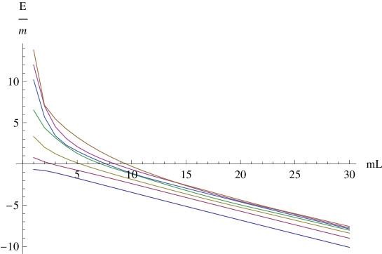
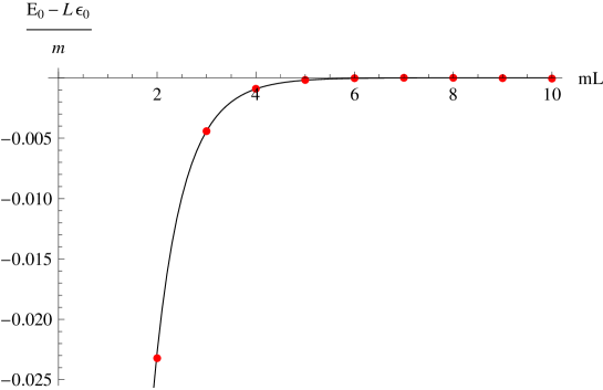
Clearly the system has a ground state energy density such that for large volumes all energy levels contain a term $E_{bulk}L$. This term can be analyzed already on the ground state, which goes as $E_{0}(L)=E_{\mathrm{bulk}}L+E_{exp}(L)$. Here $E_{exp}(L)$ is exponentially small for large $L$. We normalized the energy density to zero for the free boson with mass $m$. But once the interaction is switched on, the ground state energy density becomes a measurable physical quantity.

In measuring every quantity we should keep in mind that we determine the spectrum at various truncation levels $e_{cut}$. The dependence of the energy density on the cut-off is demonstrated on Figure 4.

Figure 4: The ground-state energy density $e_{0}(l)/l$ as the function of the volume for various truncated energy levels together with the extrapolated results. The energy density obtained at $l=7$ is indicated with a dashed line.

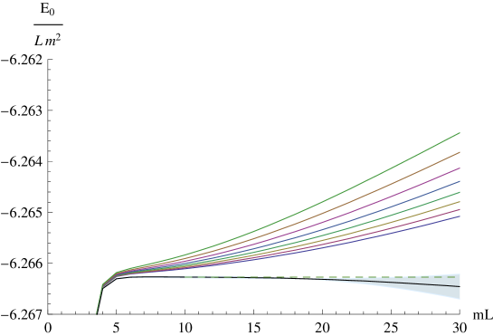
As truncation effects are very large, we have to extrapolate in the cut-off dependence in order to get a reasonable result. Based on the analysis in [13] we found it useful to fit the following function

$$E(e_{cut})=a+b\frac{\log^{2}e_{cut}}{e_{cut}^{2}}+c\frac{\log e_{cut}}{e_{cut}^{2}}$$ (77)

In order to say something about the accuracy of the extrapolation, we also fitted a simpler form

$$E(e_{cut})=a+b\frac{\log^{2}e_{cut}}{e_{cut}^{2}}$$ (78)

and used the difference of the two results for the error approximation on Figure 4.

We show on Figure 5 the convergence of the energy density values along with the fitted function.

Figure 5: Data points as a function of the truncation energy together with the fitted function for the ground-state energy density at $g=0.06$ and volume $l=10$.

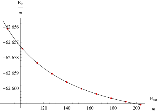
In the following we use (77) to extrapolate each energy level and show on the plots the extraploted value only. In most of the cases we subtract the vacuum energy density, such that a typical spectrum looks like the one on Figure 6.

Figure 6: Low lying spectrum at $g=0.06$: the first seven energy levels (with the vacuum energy density subtracted) are plotted against the volume in the periodic sector. The splitting of even and odd lines is so small that it is not visible at this scale.

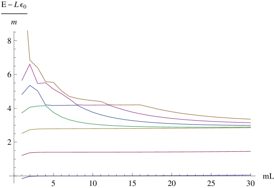
We can easily identify the first and second breathers and even a resonance around $3m_{1}$.

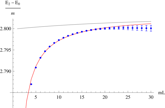
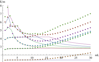
Let us start with the standing particles. For the $B_{1}$ particle the energy is a constant function of the volume up to exponential finite size corrections, however for $B_{2}$ we observed stronger finite size corrections. We blow up this part of the spectrum on Figure 7. The reason is that $B_{2}$ is a weakly coupled bound state of two $B_{1}$ particles. In decreasing the volume we pump energy into the system, which makes the bound state dissolve and behave more like two $B_{1}$ states. That is why the equation (69) with imaginary rapidities, shown by a red solid line, provides a very precise description. This fitting is very sensitive to $\alpha$, which turns out to be $\alpha=0.06$.

Figure 7: The imaginary Bethe-Yang description of $B_{2}$ at $g=0.06$, together with the leading finite size correction (shown in gray).

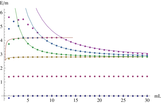
The other lines in the spectrum are described by the Bethe-Yang equations with real rapidities and quantization numbers $n=1,2,3$. These curves are shown on Figure 8.

Figure 8: Low lying even spectrum at $g=0.06$: the first six energy levels (with the vacuum energy density subtracted) are plotted against the volume together with the solid Bethe-Yang lines for $n=0,1,2,3$. The resonance is well described by a three-particle imaginary BY line including a stationary breather.

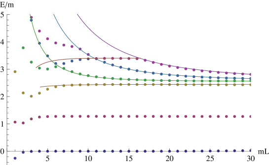
The spectrum for small $g$ can be very precisely described in a similar manner in terms of $m_{1}$ and $\alpha$. On Figure 9 we show a similar plot at $g=0.6$.

Figure 9: Low lying spectrum at $g=0.6$: the first six even energy levels (with the vacuum energy density subtracted) are plotted against the volume together with the solid Bethe-Yang lines for $n=0,1,2,3$ and the three-particle BY line for the resonance.

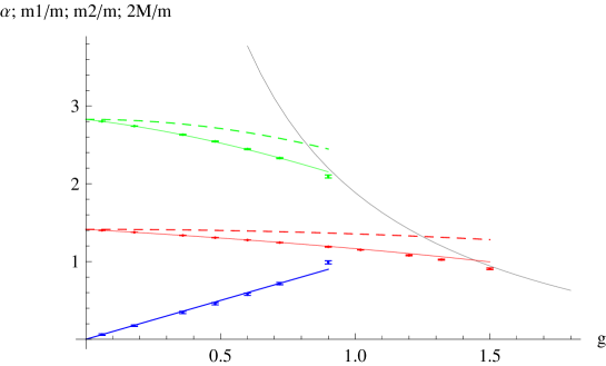
Performing a similar analysis we demonstrated for $g=0.06$ we can extract the coupling dependence of $m_{1}$, $m_{2}$ and $\alpha$. This is shown on Figure 10.

Figure 10: The masses of the breathers, $m_{1}$ (red), $m_{2}$ (green), together with the scattering parameter $\alpha$, (blue) as functions of the coupling. The numerical $B_{2}$ mass is computed using eq. (52). The semiclassical results (8,50) are indicated by dashed lines. The semiclassical result for $2M$ is shown in grey. The perturbative correction to $m_{1}$ (79) is indicated by a solid red line. The solid green line depicts $m_{2}$ as calculated by (52), using the perturbative result for $m_{1}$ and the semiclassical value of $\alpha$.

We can compare the mass of the elementary excitation to perturbation theory [14]:

$$m_{pert}^{2}(g)-m_{0}^{2}=m_{0}^{2}\left(-\frac{g}{2\sqrt{3}}-\frac{1}{36}\left(0.375+\left(2.2492+2.8020\right)-\frac{1}{2}\left(1.06864+1.9998+5.50025\right)\right)g^{2}\right)$$ (79)

Observe that the perturbative formula starts at linear order in $g$ and gives a very good approximation, opposed to the semiclassical formula, which starts at quadratic order. Having a closer look at this quantum spectrum, we can see the following: For small couplings, we have two breathers and a very heavy pair of kinks. As the coupling increases, the measured masses are smaller than the semiclassical values and the second breather disappears from the spectrum when it can decay into a kink-antikink pair, i.e. when $m_{2}(g)=2M(g)$, this happens around $g=0.9$. Similarly, the light breather, the elementary excitation of the quantum field disappears at around $g=1.5$, where its mass equals twice the mass of the kink: $m_{1}(g)=2M(g)$. For small couplings, the semiclassical calculations are reliable, which exclude the existence of more neutral particles. Indeed we can only see a resonance around $3m_{1}$. This confirms the conjecture of [19].

It is interesting to take a look at the spectrum at stronger couplings, when the breathers disappear from the spectrum.

Figure 11: Low lying spectrum at $g=1.8$: The low lying even (blue) and odd (red) energy levels (with the vacuum energy density subtracted) are plotted against the volume.

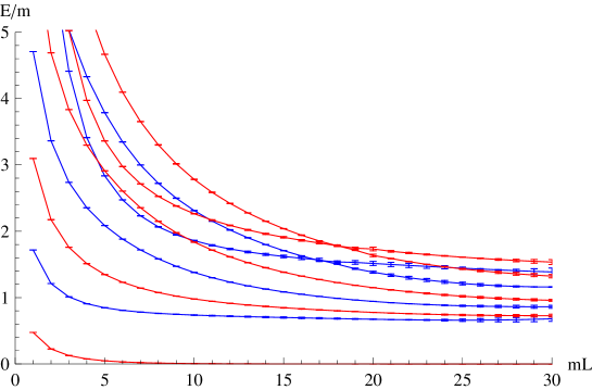
Such a spectrum is shown on Figure 11 for $g=1.8$. Clearly we can see two and four particle scattering states. By identifying the points which correspond to the two particle Bethe-Yang lines with quantization numbers $n$ and using (68,70) we can measure the $S_{k\bar{k}}$ scattering phase shift $\delta(\theta)$ as follows: We first pick up a quantization number $n$ and analyze the $E_{2}(n,L)$ curve. For a given $L$ we transform the energy using (70) to rapidity

$$E_{2}(n,L)=2M\cosh\left(\theta_{n}(L)\right)\longrightarrow\theta_{n}(L)=\cosh^{-1}\left(\frac{E_{2}(n,L)}{2M}\right)$$ (80)

We then use (68) to transform the volume for the given $\theta$ to the phase shift as:

$$-i\log S_{k\bar{k}}(2\theta)=2\pi n-ML\sinh\theta$$ (81)

Parameterizing the kink-anti-kink scattering matrix as

$$S_{k\bar{k}}(\theta)=-e^{i\delta(\theta)}$$ (82)

the resulting phase-shifts are displayed for $g=1.8$ and $g=2.4$ in Figure 12.

Figure 12: Kink-anti-kink scattering phase shifts as functions of the rapidity for $g=1.8$ (left) and for $g=2.4$ (right). The various points were extracted from lines with different $n$ in (69). For $g=1.8$ we also presented a fitted third order polynomial in $\theta$ , while for $g=2.4$ the errors of our data.

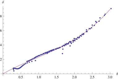
Observe that the phase shift is smaller and smaller once we increase the coupling and approach the critical point. We can fit a third order polynomial for the phase shift at $g=1.8$ as follows:

$$\delta(2\theta)=2.82(3)\,\theta-0.77(10)\,\theta^{2}+0.27(9)\,\theta^{3}$$ (83)

Clearly in the method above we needed the precise value of the kink mass. We measured this mass with two different methods: first from the splitting of the ground-state energy in subsection 6.1.2, then from the ground-state of the anti-periodic sector in section 6.2. Both measurements indicated that the kink mass is close to its semiclassical value in the whole range below the critical point, but the errors become large at stronger couplings. Therefore we used the semiclassical kink mass for these measurements. Since we do not consider the error of the kink mass, the errors are somewhat underestimated.

So far we checked only the polynomial finite size corrections. Let us investigate now the leading exponential corrections. For $g=0.06$, the mass of the lightest particle is $m_{1}=1.40182(10)$, which can be used to check the leading exponential correction of the vacuum energy (74). The comparision is shown on Figure 13, providing a convincing evidence.

Figure 13: Leading exponential correction of the vacuum energy at $g=0.06$.

The similar comparision between the energy level of the first breather and (75) indicates that we are missing some interesting physics.

Figure 14: The finite volume mass of the first breather together with the leading finite size correction (75) at $g=0.06$. $B_{1}$ energies from the rescaled TCSA spectrum of the sine-Gordon theory at $p\pi=0.06$ are also indicated by blue dots. The latter fits very well to the leading correction.

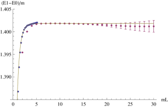
One may wonder if summing up all higher corrections coming from the elastic scattering matrix $S_{11}(\theta)=S(\theta,i\alpha)$ together with the contributions of the second breather can save the situation. To test this idea, we can compare the spectrum of our model to the spectrum of the sine-Gordon theory, at the coupling where the first breather’s scattering matrix agrees with $S_{11}(\theta)$. We used the TCSA program from [27] and rescaled the energies and volume such that the dimensionless quantities agree with this paper’s convenction. (In the TCSA program the soliton mass is normalized to $1$.) The two spectra are plotted on the same figure on Figure 15. Clearly the spectra agree very precisely for smaller volumes, when the error of the TCSA analysis is small. (We did not perform any extrapolation in the TCSA energy cut which was chosen to be $20$.) One surprising outcome is that the leading Lüscher correction (75) agrees very well with the TCSA data, but not with the $\phi^{4}$ ones. It indicates that the inelastic processes play an important role in determining the finite size effects.

Figure 15: The rescaled TCSA spectrum of the sine-Gordon theory at $p\pi=0.06$ and $e_{cut}=20$, together with the spectrum of the $\phi^{4}$ theory at $g=0.06$. The $\phi^{4}$ data are indicated by solid lines. All data are normalized wrt. the corresponding ground state energies.

6.1.2 Kink mass from the vacuum splitting

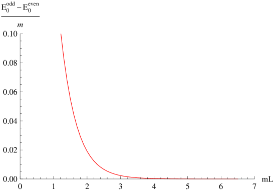
So far we analyzed the even energy levels only. To gain information about the kink mass, one can analyze the gap between the even and odd ground-state energies [27, 14]:

$$E_{0}^{even}(L)-E_{0}^{odd}(L)=\sqrt{\frac{2M}{\pi L}}e^{-ML}+\dots$$ (84)

The splitting is demonstrated on Figure 16.

Figure 16: Difference of the ground-state energies at $g=0.6$ of the even and the odd sector.

In order to extract the kink mass, we first multiply the numerical data by $\sqrt{L}$, then we measure the slope of the logarithm of the resulting curve by numerical differentiation. The result is shown on Figure 17.

Figure 17: The slope of the logarithm of the ($\sqrt{L}$-multiplied) splitting between the even and odd ground-state energies. ($g=0.6)$

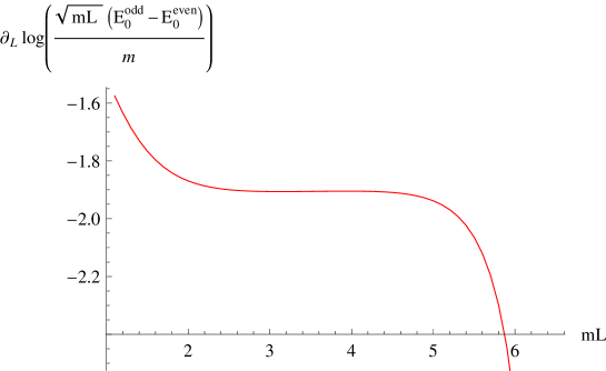
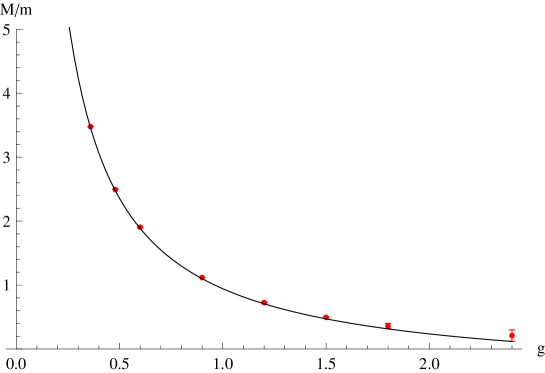
Using this analysis, we can obtain the kink mass as a function of the coupling. The curve on figure 17 seems to be monotonic. However, it actually has a little local minimum and a local maximum which can be used to estimate the error. The measured kink masses for different couplings are shown on Figure 18.

Figure 18: Kink mass as a function of the coupling extracted from the splitting together with the semiclassical result.

6.2 Antiperiodic boundary condition

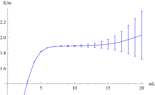
The lowest lying state in the antiperiodic sector is the kink state. After subtracting the periodic vacuum, we found the result presented on Figure 19.

Figure 19: The lowest lying state in the antiperiodic sector at $g=0.6$.

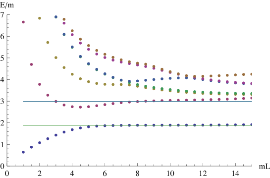
The low lying spectrum in the kink-sector is presented on Figure 20.

Figure 20: The low lying spectrum in the antiperiodic sector at $g=0.6$. We indicated the infinite volume masses of the semiclassical kink and excited kink by horizontal green and blue lines, respectively.

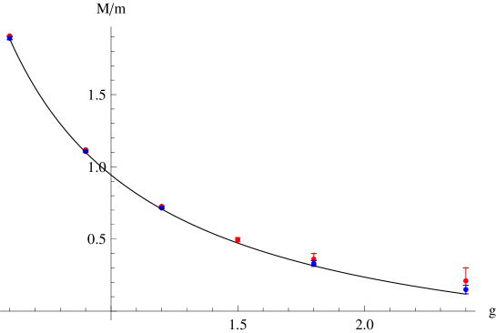
From the antiperiodic sector’s ground state we can extract the kink mass. It is in complete agreement with the one we obtained from the ground state splitting and both are very close to the semiclassical result. These data are shown on Figure 21.

Figure 21: Kink mass as a function of the coupling extracted in the antiperiodic sector (blue) together with the results from the periodic sector (red) and from semiclassical considerations (solid line).

6.3 Critical point and the spectrum of the Ising model

The vanishing of the kink mass indicates that there is a second order phase transition around $g=3$. However, increasing the coupling above $g=1.8$ renders both direct kink mass measurement methods inaccurate. On the other hand, it is known that at the critical point the spectrum must be governed by a conformal field theory, which has the spectrum

$$H_{CFT}=\frac{2\pi}{L}(L_{0}+\bar{L}_{0}-\frac{c}{12})\quad;\quad P_{CFT}=\frac{2\pi}{L}(L_{0}-\bar{L}_{0})$$

Here $L_{0}$ and $\bar{L}_{0}$ are the Virasoro generators, which measure the left and right conformal dimensions, respectively. Their sum is the scaling dimension, while their difference is the conformal spin, which is proportional to the momentum. As we analyze the zero momentum sector of the theory we list the low lying scaling dimenions of the periodic Ising model in this sector in Table 1.

state	scaling dim.	state	scaling dim.	state	scaling dim.
$|0\rangle$	$0$	$|\frac{1}{2},\frac{1}{2}\rangle\phantom{\frac{L_{L}^{L}}{L_{L}^{L}}}$	$1$	$|\frac{1}{16},\frac{1}{16}\rangle$	$\frac{1}{8}$
$L_{-2}\bar{L}_{-2}|0\rangle$	$4$	$L_{-1}\bar{L}_{-1}|\frac{1}{2},\frac{1}{2}\rangle\phantom{\frac{L_{L}^{L}}{L_{L}^{L}}}$	$3$	$L_{-1}\bar{L}_{-1}|\frac{1}{16},\frac{1}{16}\rangle$	$\frac{1}{8}+2$

Table 1: Low lying energy levels in the conformal Ising model in the zero momentum sector with periodic boundary conditions.

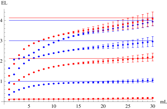
We compare this spectrum with $\frac{l}{2\pi}$ times our spectrum. First we plot the relative energies of the lowest state in the odd sector against the volume for different couplings between $g=2.76$ and $g=3.48$. This line should correspond to the $|\frac{1}{16},\frac{1}{16}\rangle$ state at the point of the phase transition. The result is shown on Figure 22. This indicates that the critical point is between $g=3.1$ and $g=3.3$.

Figure 22: Relative energies of the lowest state in the odd sector, multiplied by $l/2\pi$ for couplings g=2.76 (purple), g=2.88 (green), g=3 (orange), g=3.12 (red), g=3.24 (blue), g=3.36 (brown) and g=3.48 (gray). The line $el/(2\pi)=1/8$ is shown as a horizontal line.

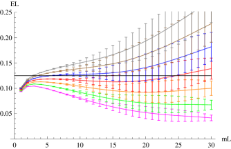
We plotted the low-lying periodic spectrum at $g=3.24$ in Figure 23. Similarly to the critical behaviour of the two-frequency sine-Gordon model [5], we nicely recover the conformal Ising spectrum. Higher energy states approach their asymptotic values later, but all the multiplicities are correct. This result is a very strong confirmation that the critical behaviour is controlled by the conformal Ising model.

Figure 23: Scaling dimensions of the periodic Ising model in the zero momentum sector (solid lines), together with our spectrum in units of $\frac{2\pi}{l}$. Blue lines and points are from the even, while red lines and points are from the odd sector.

6.4 Comparison to [14]

In this subsection we compare our methods and results to those in [14]. We focus on the periodic sector only as [14] analyzed this sector. In order to facilitate the comparison we recall that the quartic coupling in [14] is denoted by $g_{4}\equiv g_{[14]}$, while the quadratic coupling is $\frac{1}{4}M_{[14]}^{2}$. Since both papers use the same scheme, it implies that $M_{[14]}=m_{0}=\sqrt{2}m$ and $g=12\frac{g_{[14]}}{M_{[14]}^{2}}$. Consequently the dimensionless volumes are related as $l_{[14]}=M_{[14]}L=\sqrt{2}l$, while the energies as $\frac{H}{m}=\sqrt{2}\frac{H_{[14]}}{M_{[14]}}$

In the periodical case both papers used the same mini-Hilbert space approach, but the numerical implementations of improving the cut-off dependence were different. The paper [14] used a smaller Hilbert space of size $10000$ but decreased the truncation errors drastically by deriving an effective Hamiltonian, which took into account the cut-out Hilbert space in the leading non-vanishing order of the perturbation theory. (This was further improved in [15]). Contrary, we used efficient diagonalizing routines for large sparse matrices having up to $250$ million nonzero matrix elements, and extrapolated in the cut dependence following their previous work [13]. We tested this method in the symmetric sector by comparing our results to the one in [13]: We used the code in [13] to produce raw and renormalized data, which we compared to our raw and extrapolated data. At $g_{4}=1.5$, $m=1$, using an energy cut $e_{cut}=16$, the raw data agreed with high precision: the difference appearing in the fourth-fifth digit for the first eigenvalues (the truncation was slightly differently defined, so deviations were larger than the numerical precision). Our extrapolated data agreed with the renormalized data within their errors for all observables, except for the ground-state energy density, for which our data was a bit lower. Thus our method possibly slightly overextrapolates. For this reason, in the future we are planning to combine the two methods.

In comparing the results we note that we managed to analyze the model in a wider parameter range than [14]. For the overlapping parameters we found agreement within the numerical errors. For large couplings we identified the critical point $g=3.2\left(1\right)$, which agrees with their findings using Chang duality. Since the numerical errors grow with the volume we put emphasis on the finite size spectrum including all polynomial and the leading exponential corrections. We did it in all sectors of the theory. In measuring the kink mass via the vacuum splitting we fitted their finite size formula. Having a good control of the finite size effects enabled us to extract physical information from the volume range $l=[5,15]$ where both the exponential theoretical corrections and the numerical errors were small.

7 Conclusions

In this paper we investigated the two dimensional $\phi^{4}$ theory in the broken phase by the massive generalization of the truncated conformal space approach. We called this method the truncated Hilbert space approach and we developed a code based on the diagonalization of large sparse matrices to diagonalize the truncated dimensionless Hamiltonian. We determined the spectrum numerically for various volumes and quartic couplings and both for periodic and antiperiodic boundary conditions. In the periodic case we found it useful to adapt the mini superspace approach. We compared the results with semiclassical calculations and also with finite size corrections. These finite size corrections are expressed in terms of the infinite volume masses and scattering matrices, for which we proposed parametrizations from the unitarity relations. We summarized the infinite volume mass spectrum and scattering parameter as functions of the coupling on Figure 24.

Figure 24: The mass spectrum of the model as function of the coupling $g$. The mass of the breathers, $m_{1}$ (red), $m_{2}$ (green), together with the scattering parameter $\alpha$, (blue). The numerical $B_{2}$ mass is computed using eq. (52). The semiclassical results (8,50) are indicated by dashed lines. The semiclassical result for the kink mass is shown in grey, while the one determined from the vacuum splitting by black and the one determined from the anti-periodical sector by orange. The semiclassical excited kink is shown in brown. The perturbative correction to $m_{1}$ (79) is indicated by a solid red line. The solid green line depicts $m_{2}$ as calculated by (52), using the perturbative result for $m_{1}$ and the semiclassical value of $\alpha$.

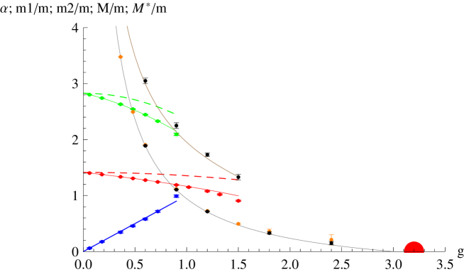
We found a very good agreement with the semiclassical results for the breather spectrum for moderate couplings. We then mapped the full spectrum of the neutral and kink excitations. We found at most two neutral excitations and each particle disappeared from the spectrum when its mass exceeded twice the mass of the lightest particle. This confirms the conjecture of [19] that only two neutral excitations can exist in the spectrum.

In determining the kink mass we used both the splitting of the even and odd ground-state energies with periodical boundary conditions and also the lowest lying state in the antiperiodic sector. These two methods agreed very well and the results were close to the semiclassical spectrum. For large couplings we identified the critical point beyond which the broken $\mathbb{Z}_{2}$ symmetry is restored. We also confirmed that the second order phase transition is within the Ising universality class. In computing the leading exponential mass correction of the lightest neutral excitation we found relevant deviations from the Lüscher formula (75). By comparing the spectrum with the analogue breather spectrum of the sine-Gordon theory we got convinced that this effect must be attributed to non-integrable, inelastic processes, which need to be understood further.

We believe that improving our data with the renormalization group method of [13] enables to measure other interesting quantities such as decay rates or the inelastic part of the scattering matrices.

Another interesting direction of research is to describe the strongly coupled spectrum by perturbing the conformal Ising model and to compare the analytical results to the improved numerics.

Appendix A Ground-state energy from normal ordering

In this Appendix we motivate the ground-state energy

$$E_{0}(\mu,L)=\mu\int_{-\infty}^{\infty}\frac{d\theta}{2\pi}\cosh\theta\log(1-e^{-mL\cosh\theta})$$ (85)

of the free massive boson from a normal ordering prescription. The free normal ordered Hamiltonian in volume $L$ takes the form

$$H^{\mu,L}=\frac{1}{2}\int_{0}^{L}:(\partial_{t}\phi)^{2}+(\partial_{x}\phi)^{2}+\mu^{2}\phi^{2}:_{\mu,L}$$ (86)

Normal ordering is understood that we expand $\phi$ as

$$\phi(x,t)=\sum_{n}\frac{1}{\sqrt{2\omega_{n}L}}\left(a_{n}e^{-i\omega_{n}t+ik_{n}x}+a_{n}^{+}e^{i\omega_{n}t-ik_{n}x}\right)$$ (87)

with $\omega_{n}=\sqrt{\mu^{2}+k_{n}^{2}}$ and $k_{n}=\frac{2\pi n}{L}$ and then put all the annihilation operators $a_{n}$ on the right of the creation operators $a_{n}^{+}$ using the rule

$$[a_{n},a_{m}]=[a_{n}^{+},a_{m}^{+}]=0\quad;\qquad[a_{n},a_{m}^{+}]=\delta_{n,m}$$ (88)

This implies that

$$\phi^{2} = :\!\phi^{2}\!:_{\mu,L}+Z(\mu,L)\quad;\qquad Z(\mu,L)=\sum_{|n|<N}\frac{1}{2\omega_{n}L}$$ (89)

$$(\partial_{t}\phi)^{2} = :\!(\partial_{t}\phi)^{2}\!:_{\mu,L}+Y_{t}(\mu,L)\quad;\qquad Y_{t}(\mu,L)=\sum_{|n|<N}\frac{\omega_{n}^{2}}{2L\omega_{n}}$$ (90)

$$(\partial_{x}\phi)^{2} = :\!(\partial_{x}\phi)^{2}\!:_{\mu,L}+Y_{x}(\mu,L)\quad;\qquad Y_{x}(\mu,L)=\sum_{|n|<N}\frac{k_{n}^{2}}{2L\omega_{n}}$$ (91)

where we introduced a cut-off to make them finite.

In the paper we are interested in the following perturbation of the system

$$H=H^{\mu,L}+\frac{\delta\mu^{2}}{2}\int_{0}^{L}:\phi^{2}:_{\mu,L}dx=\frac{1}{2}\int_{0}^{L}:(\partial_{t}\phi)^{2}+(\partial_{x}\phi)^{2}+\mu^{\prime 2}\phi^{2}:_{\mu,L}$$ (92)

where $\mu^{\prime 2}=\mu^{2}+\delta\mu^{2}$. We would like to understand in which way it is related to $H^{\mu^{\prime},L}$. They formally look the same – however, they are normal ordered at different mass scales. As a result, they differ by a constant term. To calculate this constant, we use

$$:\!\phi^{2}\!:_{\mu,L} = :\!\phi^{2}\!:_{\mu^{\prime},L}+\Delta Z\quad;\qquad\Delta Z=\frac{1}{2L}\sum_{n}\left(\frac{1}{\omega^{\prime}_{n}}-\frac{1}{\omega_{n}}\right)$$ (93)

$$:\!(\partial\phi)^{2}\!:_{\mu,L} = :\!(\partial\phi)^{2}\!:_{\mu^{\prime},L^{\prime}}+\Delta Y\quad;\qquad\Delta Y=\frac{1}{2L}\sum_{n}\left(\frac{(\omega^{\prime}_{n})^{2}+k_{n}^{2}}{\omega^{\prime}_{n}}-\frac{\omega{}_{n}^{2}+k_{n}^{2}}{\omega{}_{n}}\right)$$

where $\omega^{\prime}_{n}=\sqrt{\mu^{\prime 2}+k_{n}^{2}}$ and $(\partial\phi)^{2}=(\partial_{t}\phi)^{2}+(\partial_{x}\phi)^{2}$. Observe that all the sums are finite, although this would not be true separately for $(\partial_{t}\phi)^{2}$ or for $(\partial_{x}\phi)^{2}$. In the first term we can subtract the infinite volume limit

$$Z(\mu^{\prime},\infty)-Z(\mu,\infty)=\int_{-\infty}^{+\infty}\frac{dk}{4\pi}\left(\frac{1}{\sqrt{\mu^{\prime 2}+k^{2}}}-\frac{1}{\sqrt{\mu^{2}+k^{2}}}\right)=-\frac{1}{2\pi}\log\frac{\mu^{\prime}}{\mu}$$ (94)

to obtain

$$\Delta Z=Z(\mu^{\prime},L)-Z(\mu,L)=z(\mu^{\prime}L)-z(\mu L)-\frac{1}{2\pi}\log\frac{\mu^{\prime}}{\mu}$$ (95)

where

$$z(\mu L)=Z(\mu,L)-Z(\mu,\infty)=\int_{0}^{\infty}\frac{d\theta}{\pi}(e^{\mu L\cosh\theta}-1)^{-1}$$ (96)

Similarly,

$$Y(\mu^{\prime},\infty)-Y(\mu,\infty)=\int_{-\infty}^{+\infty}\frac{dk}{4\pi}\left(\frac{\mu^{\prime 2}+2k^{2}}{\sqrt{\mu^{\prime 2}+k^{2}}}-\frac{\mu^{2}+2k^{2}}{\sqrt{\mu^{2}+k^{2}}}\right)=\frac{1}{4\pi}\left(\mu^{\prime 2}-\mu^{2}\right)$$ (97)

so that we get

$$\Delta Y=\frac{2E_{0}(\mu^{\prime},L)}{L}-\frac{2E_{0}(\mu,L)}{L}-\mu^{\prime 2}z(\mu^{\prime}L)+\mu^{2}z(\mu L)+\frac{1}{4\pi}\left(\mu^{\prime 2}-\mu^{2}\right)$$ (98)

This implies that

$$H^{\mu,L}+\frac{\delta\mu^{2}}{2}\int_{0}^{L}:\phi^{2}:_{\mu,L}dx=H^{\mu^{\prime},L}+E_{0}(\mu^{\prime},L)-E_{0}(\mu,L)-\frac{\delta\mu^{2}}{2}Lz(\mu L)+L\left[\frac{1}{8\pi}(\mu^{\prime 2}-\mu^{2})-\frac{\mu^{\prime 2}}{4\pi}\log\frac{\mu^{\prime}}{\mu}\right]$$ (99)

We can reformulate this result as

$$H^{\mu,L}+E_{0}(\mu,L)+LE_{bulk}(\mu)+\frac{\delta\mu^{2}}{2}\int_{0}^{L}\left(:\phi^{2}:_{\mu,\infty}-\frac{1}{2\pi}\log\mu\right)dx=H^{\mu^{\prime},L}+E_{0}(\mu^{\prime},L)+LE_{bulk}(\mu^{\prime})$$ (100)

That is, if we normal order the interaction term at infinite volume and introduce the ground-state energy by $E_{0}(\mu,L)$ and ground-state energy density by $E_{bulk}(\mu)=\frac{\mu^{2}}{8\pi}-\frac{\mu^{2}}{4\pi}\log\mu$ then the perturbation will change these parameters in a consistent way. In the following, we do not keep track of the energy density and introduce the perturbing operator simply as $:\phi^{2}:_{\mu,\infty}$.

One can also wonder how the ground state energy changes by changing the volume, i.e. to relate the system with mass $\mu$ and volume $L$ to the same system with volume $L^{\prime}$. Clearly the spectrum of the two systems are completely different. What we can compare is the ground state energy. We will demand that $LH$ depends only on $\mu L$. This is satisfied for

$$LH^{\mu,L}+LE_{0}(\mu,L)=\frac{1}{2}\sum_{k}\sqrt{(\mu L)^{2}+4\pi^{2}n^{2}}+\mu L\int_{-\infty}^{\infty}\frac{d\theta}{2\pi}\cosh\theta\log(1-e^{-\mu L\cosh\theta})$$ (101)

This implies that

$$LH^{\mu,L}+LE_{0}(\mu,L)=L^{\prime}H^{\mu^{\prime},L^{\prime}}+L^{\prime}E_{0}(\mu^{\prime},L^{\prime})\quad;\qquad\mu L=\mu^{\prime}L^{\prime}$$ (102)

By this rule we can calulate the ground state energy at volume $L^{\prime}$ and mass $\mu$.

Summarising, the vacuum energy at volume $L$ and renormalization scale $\mu$ is $E_{0}(\mu,L)$, which is independent of the path we arrive at this point, i.e. by adding perturbations or by changing the volume. But we do not keep track of the change in the vacuum energy density.

Appendix B Parametrizing the scattering matrix

Here we analyze the $2\to 2$ scattering matrices of the theory. We first recall how the unitarity of the scattering matrix can be used to gain information on its analytic structrure. The idea is to write the unitarity equation $SS^{\dagger}=\mathbb{I}$ for the interaction part of the matrix $S=\mathbb{I}+iT$ as

$$i(T-T^{\dagger})=-TT^{\dagger}$$ (103)

Taking matrix element between initial and final states and inserting a complete system we can write

$$\langle out|i(T-T^{\dagger})|in\rangle=-\sum_{n\in\mathcal{H}}\langle out|T|n\rangle\langle n|T^{\dagger}|in\rangle$$ (104)

For diagonal matrix elements, this equation implies the optical theorem, namely the absolute square of the total cross section is related to the imaginary part of the forward scattering amplitude. This equation shows that S-matrix elements are not independent, they are connected analytically by a very intrinsic way.

Let us focus on the $2\to 2$ particle scattering process and denote the momenta of the initial particles as $p_{1},p_{2}$ and outgoing particles as $p_{3},p_{4}$ , which are all onshell $p_{i}^{2}=\omega_{i}^{2}-k_{i}^{2}=m_{1}^{2}$. Energy conservation can be factored out

$$\langle p_{3},p_{4}|S|p_{1},p_{2}\rangle\propto(2\pi)^{2}\delta^{(2)}(p_{1}+p_{2}-p_{3}-p_{4})S(s,t,u)$$ (105)

where due to relativistic invariance the scattering matrix depends on the Mandelstam variables

$$s=(p_{1}+p_{2})^{2}\quad;\qquad t=(p_{1}-p_{3})^{2}\quad;\qquad u=(p_{1}-p_{4})^{2}$$ (106)

On-shell condition implies that $s+t+u=4m_{1}^{2}$. In two dimension the kinematics is further restricted since $t=4m^{2}-s$. The analytical S-matrix theory states that $S(s)$ can have poles and cuts dictated by unitarity, but otherwise it is an analytical function of $s$, which also satisfies crossing symmetry. Spelling out the equation (104) for the two-particle process we obtain:

$$\langle p_{3},p_{4}|i(T-T^{\dagger})|p_{1},p_{2}\rangle=-\sum_{n\in\mathcal{H}}\langle p_{3},p_{4}|T|n\rangle\langle n|T^{\dagger}|p_{1},p_{2}\rangle$$ (107)

In factoring out momentum coservation we assume that $k_{1}>k_{2}$ and $k_{3}>k_{4}$ such that $k_{1}=k_{3}$ and $k_{2}=k_{4}$ must hold. Let us write out the first few terms. Clearly the vacuum does not contribute. The one- and two-particle contributions read as

$$2\Re eS(s,t) = \int dk_{n}\delta^{(2)}(p_{1}+p_{2}-p_{n})\Gamma_{12}^{n}\Gamma_{n}^{34}+$$

$$\int dk_{n_{1}}dk_{n_{2}}\delta^{(2)}(p_{1}+p_{2}-p_{n_{1}}-p_{n_{2}})S(p_{1},p_{2},p_{n_{1}},p_{n_{2}})S(p_{n_{1}},p_{n_{2}},p_{3},p_{4})+\dots$$

Here we factored out the total energy momentum conservation. However, on the rhs. other $\delta$ functions appeared, which eat up one integration leading to an energy delta function in the one-particle and a constant piece in the two-particle contribution. Since these contributions appear only for certain analytically continued values of $s$, they tell us the non-analytical positions of the scattering matrix on the complex $s$-plane. Bound states correspond to poles, where energy conservation can be maintained, and the two-particle threshold gives a cut starting from $s=4m_{1}^{2}$.

Let us go into the center of mass frame $k_{1}\equiv k=-k_{2}$. Then we have $s=4m_{1}^{2}+4k^{2}$ and $t=-4k^{2}$, such that relation $t=4m_{1}^{2}-s$ is satisfied. Crossing symmetry implies that

$$S(s+i\epsilon)=S(t+i\epsilon)=S(4m_{1}^{2}-s-i\epsilon)$$ (109)

Switching from the $i\epsilon$ prescription to the $-i\epsilon$ prescription is equivalent to time reversal, which changes the scattering matrix to its inverse

$$S(s+i\epsilon)=S(s-i\epsilon)^{-1}$$ (110)

The analytical structure of the S-matrix is displayed on the following figure:

The bound state poles are at $m_{2}^{2}$ and at $4m_{1}^{2}-m_{2}^{2}$. There are cuts on the real line starting at the multiparticle thresholds $(m_{n}+m_{k}+\dots)^{2}$. The physical value of the S-matrix is at $S(s+i\epsilon)$ where $s>4m_{1}^{2}$.

In the following we parametrize the two-particle scattering matrix based on this analytical structure. We first switch to rapidity parametrization. In the center of mass frame $k_{1}=-k_{2}=m\sinh\frac{\theta}{2}$, such that the rapidity difference is $\theta$. The rapidity is related to the $s$ variable as

$$s=4m_{1}^{2}(1+\sinh^{2}\frac{\theta}{2})=4m_{1}^{2}\cosh^{2}\frac{\theta}{2}$$ (111)

This resolves the cut starting at $4m_{1}^{2}$ and maps the first sheet of the complex $s$-plane to the strip $0<\Im m(\theta)<\pi$. The bound state poles are located on the imaginary axes at $\theta=i\zeta$ and at $\theta=i(\pi-\zeta)$, since

$$m_{2}^{2}=4m_{1}^{2}\cos^{2}\frac{\zeta}{2}$$ (112)

The first branch cut depends on the masses. Assuming the kinks are very heavy they appear at $s=(m_{1}+m_{2})^{2}$ or in the rapditity parameter at $\theta_{t}$:

$$\cosh\frac{\theta_{t}}{2}=\frac{1}{2}(1+\frac{m_{2}}{m_{1}})=\frac{1}{2}\bigl{(}1+2\cos\frac{\zeta}{2}\bigr{)}$$ (113)

If the kinks are lighter, then even earlier. Now we turn this information into a parametrization of the scattering matrix. Recall that crossing symmetry translates to the rapidity parameter as

$$S(i\pi-\theta)=S(\theta)$$ (114)

while the S-matrices on the two sides of the cut are related as

$$S(\theta)=S(-\theta)^{-1}.$$ (115)

In order to have the right periodicity and good asymptotic behaviour let us consider the logarithmic derivative of the scattering matrix:

$$\phi(\theta)=\frac{d}{d\theta}\log S(\theta)$$ (116)

It has the properties

$$\phi(\theta)=\phi(-\theta)\quad;\qquad\phi(\theta)=-\phi(i\pi-\theta)=-\phi(i\pi+\theta)$$ (117)

Let us write it as

$$\phi(\theta)=\oint_{\theta}\frac{d\theta^{\prime}}{2\pi i}\frac{\phi(\theta^{\prime})}{\sinh(\theta^{\prime}-\theta)}$$ (118)

where the contour sorrounds infinitesimally $\theta$. Now we blow up the contour and deform it to $\theta=0$ above the cuts and to $\theta=i\pi$ below the cuts. In doing so we pick up the residues of the bound state poles:

$$\phi(\theta)=\frac{1}{\sinh(i\zeta-\theta))}+\frac{1}{\sinh(i(\pi-\zeta)-\theta)}-\int_{\theta_{t}}^{\infty}\frac{d\theta^{\prime}}{2\pi i}\rho(\theta^{\prime})\left(\frac{1}{\sinh(\theta^{\prime}-\theta)}+\frac{1}{\sinh(i\pi-\theta^{\prime}-\theta)}\right)$$ (119)

where $\rho(\theta)$ is the jump of $\phi(\theta)$ on the cut, which is related to the inelastic scattering processes through the unitarity relation. After integrating and exponentiating we obtain

$$S(\theta)=S(\theta,i\zeta)\exp\left\{-\int_{\theta_{t}}^{\infty}\frac{d\theta^{\prime}}{2\pi i}\rho(\theta^{\prime})\log S(\theta^{\prime},\theta)\right\}\quad;\qquad S(\theta,x)=\frac{\sinh\theta+\sinh x}{\sinh\theta-\sinh x}$$ (120)

where we made the integral to converge for large $\theta^{\prime}$. We note that similar parametrization should be valid for the kink-kink and kink-breather scattering matrices.

Appendix C A review of the numerical algorithm used

In this Appendix we review the numerical implementation of our method.

C.1 Overview

The numerical results were obtained using an application written in C++, that is supplied with this document. We tested the simulation under SuSe and Ubuntu Linux platforms.

As explained earlier,the matrix elements of the Hamiltonian are calculated in a truncated, finite-dimensional basis and then the lowest eigenvalues of the obtained large sparse matrix is determined. With the use of the PRIMME iterative eigensolver package[28] (of which we currently use version 1.1), it was possible to work with matrices of up to $250$ million nonzero mattix elements on a single personal computer, the computing time being a couple of minutes per measurement point. The eigensolver uses an improved version of the Jacobi-Davidson method (referred as JDQMR_ETOL in PRIMME).

The algorithm itself is generally capable of handling a Hamiltonian composed of the sum of a finite number of Landau-Ginzburg interactions in 1+1 dimensions put into a finite volume. In this article, we focused on the parity-conserving $\varphi^{4}$ model, and thus the parameter corrections are only implemented to this case. In the periodic sector, it proved to be sufficient to use the minimal Hilbert-space approach, with the separate treatment of the zero mode and the construcion of the overall Hamiltonian as a direct product of the minimal and non-minimal subspaces. An emphasis was also put on the antiperiodic sector, though obviously the minimal space approach is not applicable in this case.

A single run of the program usually generates several output files, each one corresponding to a different energy cutoff. A single file contains the relevant eigenvalues for different volumes between a minimal volume $L_{min}$ and maximal volume $L_{max}$, having step $L_{step}$, the interaction strength parameters being corrected corresponding to the change of volume, while all other parameters are kept fixed.

The parameters of the simulations can be set in a separate configuration file, in which the user can set the number of eigenvalues to be calculated, along with the interaction strengths, truncation dimensions, and output file name. It is possible there to decide the usage of the minimal space method, choose the boundary condition and select the desired parity and momentum sector. A basis mass and volume must also be given for the construction of the free Fock basis. The examined volume interval and step size are also to be given in the aforementioned file.

The source code is structured around C++ classes and is divided into several files. The entry point of the program is in the file main.cpp. Some auxiliary routines and numerical functions are declared and defined in utils.h and utils.cpp. A numerical integration routine from Numerical Recipes[29] is implemented in numint.cpp. The classes HilbertState and HilbertSpace, which are used to build the Fock basis, are defined in phi4.cpp. The algorithms regarding the calculation of a Landau-Ginzburg interaction term between two Fock states are implemented in phi_n.cpp. The class Hamiltonian is realized in minspace.h and minspace.cpp. A class to store a sparse matrix in coordinate list (COO) format is defined in coo.cpp, along with a number of routines particularly useful for our considerations. The header primme.h provides the interface to PRIMME functions. The connection between the simulation and the eigensolver is realised in the utility functions of PRIMME_int.h. Most notably, as PRIMME uses a different sparse matrix format (Compressed Sparse Row, CSR), there is a routine to convert the COO format sparse matrix to one that is operable by the eigensolver.

C.2 The basis

A state of the Fock space is represented by the class HilbertState in the algorithm. In fact, the particle content can be written in conventional representation

$$\left|u\right\rangle=\left|\left(k_{1},n_{1}\right),\left(k_{2},n_{2}\right),\dots\left(k_{r},n_{r}\right)\right\rangle$$

where this notation stands for having a state $\left|u\right\rangle$ that contains a number $n_{1}$ of particles with momentum $k_{1}$, and a number $n_{2}$ of particles with momentum $k_{2}$, and so on, until all particles are counted for in the state. Due to the finite volume, the momenta are quantized so that in the periodic sector:

$$k_{m}=\frac{\pi}{L}\left(2m\right),\quad m\in\mathbb{Z},$$

while in the antiperiodic sector,

$$k_{m}=\frac{\pi}{L}\left(2m+1\right),\quad m\in\mathbb{Z}_{-};\qquad k_{m}=\frac{\pi}{L}\left(2m-1\right).\quad m\in\mathbb{Z}_{+}$$

Any Fock vector is thus identified by a finite series of integer pairs. A series like this can be stored in a variable of type HilbertState.

The HilbertSpace class contains an array of HilbertState variables. Crucially, this array is filled by a member function in a determined way, so that the HilbertSpace contains all Fock vectors below a given energy cutoff. Starting from an auxiliary vacuum state (a HilbertState variable that is empty), the construction is performed recursively, each recursive step having two parts: first we add an additional particle of some momentum $i$ to the auxiliary Fock state containing only particles with positive momenta. Then we distribute the signs of particle momenta every possible way so that the overall momentum lies in the appropriate sector. The construction routine is called with a starting auxiliary state, and has a loop in which the function calls itself with another auxilary state having one additional particle. If the energy cut is reached, the loop breaks and the routine returns. If the embedded routine returns, the momentum i of the added particle gets increased. At the end, the members of the array get sorted according to their energy (with respect to the basis volume and mass).

The truncation of basis is also implemented in the HilbertSpace class; it corresponds to cutting off the highest energy states from the array.

C.3 Calculating interaction matrix elements

Due to the remarkable efficiency of the eigensolver routine, the construction of the sparse matrix and evaluation of matrix elements can also turn out to be the bottleneck of computation speed. The algorithm was designed to fit two criteria: firstly it should be able to decide very quickly if a matrix element is zero or not, and secondly, it should calculate the actual values of matrix elements as effectively as possible.

A Landau-Ginzburg interaction term of degree $N$ reads

$$\mathcal{O}_{N}=g_{N}\intop_{0}^{L}:\varphi\left(x,t\right)^{N}:dx=g_{N}\frac{1}{2^{N/2}L^{N/2-1}}\sum_{\left\{k_{i},\epsilon_{i}\right\}}\frac{:\prod_{i=1}^{N}a_{k_{i}}^{\epsilon_{i}}:}{\sqrt{\prod_{i=1}^{N}\omega_{n_{i}}}}\left(\delta_{\sum_{i=1}^{N}\epsilon_{i}k_{i}}\right)$$ (121)

where $k_{i}$ runs through the one-particle momenta allowed by the boundary condition, $\epsilon=\pm 1$, $a_{n}^{+1}\equiv a_{n}^{+}$, and $a_{n}^{-1}\equiv a_{n}$.

First it should be noted that the matrix element $\left\langle a\right|\mathcal{O}_{N}\left|b\right\rangle$ can have a nonzero value only if the state $\left|b\right\rangle$ can be transformed into a state equivalent of $\left|a\right\rangle$ by a product of at most $N$ creation-annihilation opeators. Therefore the problem of fast discrimination of zero matrix elements reduces to using the particle content of $\left|a\right\rangle$ to generate all states $\left|b\right\rangle$ with energy $E_{\left|b\right\rangle}\leq E_{\left|a\right\rangle}$ and $\left\langle a\right|\mathcal{O}_{N}\left|b\right\rangle\neq 0$ and looking them up in the array of HilbertStates. Secondly, the actual content difference of $\left|a\right\rangle$ and $\left|b\right\rangle$ determines which operator product terms from the sum in (121) contribute to the matrix element. (Since the simulation imposes normal ordering at the volume of computation, we don’t have to consider terms of “tadpole” type, where new particles not contained in any of the states would pop up and annihilate each other.)

The determination of the content difference is facilitated by the class StateDifference. This structure contains two arrays: the first array lists the momentum of all particles in the bra vector that are not present in the ket vector; the secod contains the particles only present in the ket vector. The sum of array sizes gives the total number of creation-annihilation operators needed to transform the states into each other. This total number will be called particle difference for simplicity. The comparison of the two HilbertSpace variables and the construction of these arrays is done by a constructor of StateDifference.

If the particle difference of two HilbertStates is exactly $N$, then there is only one type of contributing normal ordered operator product from (121). However, if we only count operator product terms that are different after normal ordering, we always have to remember that the action of normal ordering effectively produces a multinomial coefficient for each term. If the particle difference is a value $N_{pd}<N$, then we may also annihilate and create $N-N_{pd}$ particles taken arbitarily from the ket vector. Since the matrix is symmetric, we can interchange the bra and ket vector so that the number of annihilation operators is always greater or equal than the number of creation operators in the term under consideration. Thus every contributing term can be accounted for by examining the ket vector particle content and the particle difference. The contributions to the matrix element of $\mathcal{O}_{n}$ are then calculated term by term. This computation is done for a single $\mathcal{O}_{N}$ term using the class phi_n_interaction.

C.4 The Hamiltonian

As mentioned earlier, the matrix representation of the truncated Hamiltonian in the generated Fock basis is stored in a sparse matrix. The matrix is technically stored in a variable of type sparse_matrix. A single matrix element is kept in a struct variable such that the row and column index is stored explicitly along with the value of the element. Tha class sparse_matrix consists of an array of these structs, along with some useful member functions.

The interactive part of the Hamiltonian consists of a sum of terms $\mathcal{O}_{N}$ in the form (121). The parameter corrections according to the scheme change are accounted for in the main function of the program.

The Hamilton operator is technically realized by a class Hamiltonian in the program. If the minimal space approach is not used, then at the beginning of the calculation, the matrix is filled with the matrix elements of the interaction, the non-diagonal ones being only saved if they are nonzero. In the Fock basis, the free Hamiltonian is diagonal, and its matrix elements are also added to the matrix. After this initial construction, only the nonzero matrix elements are modified.

C.4.1 Minimal space approach

If this approach is used, the program initially calculates the normalized (i.e. $g_{N}=1$) matrix elements of $\mathcal{O}_{N}$ between non-minimal basis states for every positive $N$ smaller or equal than the maximal interaction exponent appearing in the Hamilton operator, and store the representations in an array of sparse matrices contained in the class Hamiltonian.

For each examined volume, the minimal space spanned by zero modes are accounted for first. This basically corresponds to solving an anharmonic oscillator with appropriate coefficients and obtaining the first eigenvalues and eigenvectors in the free basis. The $\varphi^{0}$ terms of the interaction are accounted for in the minimal space calculation. As a second step, the matrix elements of interaction terms $\mathcal{O}_{N}$ are calculated between the numerically determined “exact” eigenvectors in the minimal space, and get stored as an array of (dense) matrices. Then the non-minimal (normalized) matrix elements of every $\mathcal{O}_{N}$ get actualised in the stored array of sparse matrices. In the last step, the representation of the truncated Hamilton-operator is obtained as a sum of direct product terms according to (44).

If the computation is limited to a single parity sector, then the zero-mode oscillator is calculated separately in the even and odd particle number basis. The minimal-space $\mathcal{O}_{N}$ matrices in the exact basis are constructed so that the basis vectors containing an even number of particles are ahead of those having an odd number of particles. Then the non-minimal representations of $\mathcal{O}_{N}$s are also transformed so that the even basis elements are ahead of the odd basis elements. Then the overall Hamiltonian is built up in the desired sector using the appropriate submatrices.

References

- [1] V. P. Yurov and A. B. Zamolodchikov, “Truncated conformal space approach to the scaling Lee-Yang model,” Int. J. Mod. Phys. A5 (1990) 3221–3246.
- [2] G. Feverati, F. Ravanini, and G. Takacs, “Truncated conformal space at c = 1, nonlinear integral equation and quantization rules for multi - soliton states,” Phys. Lett. B430 (1998) 264–273, arXiv:hep-th/9803104 [hep-th].
- [3] M. Beria, G. P. Brandino, L. Lepori, R. M. Konik, and G. Sierra, “Truncated Conformal Space Approach for Perturbed Wess-Zumino-Witten Models,” Nucl. Phys. B877 (2013) 457–483, arXiv:1301.0084 [hep-th].
- [4] R. M. Konik, T. Palmai, G. Takacs, and A. M. Tsvelik, “Studying the perturbed Wess-Zumino-Novikov-Witten theory using the truncated conformal spectrum approach,” Nucl. Phys. B899 (2015) 547–569, arXiv:1505.03860 [cond-mat.str-el].
- [5] Z. Bajnok, L. Palla, G. Takacs, and F. Wagner, “Nonperturbative study of the two frequency sine-Gordon model,” Nucl. Phys. B601 (2001) 503–538, arXiv:hep-th/0008066 [hep-th].
- [6] B. Pozsgay and G. Takacs, “Characterization of resonances using finite size effects,” Nucl. Phys. B748 (2006) 485–523, arXiv:hep-th/0604022 [hep-th].
- [7] B. Pozsgay and G. Takacs, “Form-factors in finite volume I: Form-factor bootstrap and truncated conformal space,” Nucl. Phys. B788 (2008) 167–208, arXiv:0706.1445 [hep-th].
- [8] G. Takacs and G. Watts, “Excited State G-Functions from the Truncated Conformal Space,” JHEP 02 (2012) 082, arXiv:1112.2906 [hep-th].
- [9] Z. Bajnok, L. Palla, G. Takacs, and G. Z. Toth, “The Spectrum of boundary states in sine-Gordon model with integrable boundary conditions,” Nucl. Phys. B622 (2002) 548–564, arXiv:hep-th/0106070 [hep-th].
- [10] Z. Bajnok, L. Hollo, and G. Watts, “Defect scaling Lee-Yang model from the perturbed DCFT point of view,” Nucl. Phys. B886 (2014) 93–124, arXiv:1307.4536 [hep-th].
- [11] M. Hogervorst, S. Rychkov, and B. C. van Rees, “Truncated conformal space approach in d dimensions: A cheap alternative to lattice field theory?,” Phys. Rev. D91 (2015) 025005, arXiv:1409.1581 [hep-th].
- [12] A. Coser, M. Beria, G. P. Brandino, R. M. Konik, and G. Mussardo, “Truncated Conformal Space Approach for 2D Landau-Ginzburg Theories,” J. Stat. Mech. 1412 (2014) P12010, arXiv:1409.1494 [hep-th].
- [13] S. Rychkov and L. G. Vitale, “Hamiltonian truncation study of the theory in two dimensions,” Phys. Rev. D91 no. 8, (2015) 085011, arXiv:1412.3460 [hep-th].
- [14] S. Rychkov and L. G. Vitale, “Hamiltonian truncation study of the theory in two dimensions. II. The -broken phase and the Chang duality,” Phys. Rev. D93 no. 6, (2016) 065014, arXiv:1512.00493 [hep-th].
- [15] J. Elias-Miro, M. Montull, and M. Riembau, “The renormalized Hamiltonian truncation method in the large expansion,” arXiv:1512.05746 [hep-th].
- [16] R. Rajaraman, Solitons and Instantons. An introduction to solitons and instantons in quantum field theory. 1982.
- [17] R. F. Dashen, B. Hasslacher, and A. Neveu, “Nonperturbative Methods and Extended Hadron Models in Field Theory. 2. Two-Dimensional Models and Extended Hadrons,” Phys. Rev. D10 (1974) 4130–4138.
- [18] G. Fodor, P. Forgacs, Z. Horvath, and A. Lukacs, “Small amplitude quasi-breathers and oscillons,” Phys. Rev. D78 (2008) 025003, arXiv:0802.3525 [hep-th].
- [19] G. Mussardo, “Neutral Bound States in Kink-like Theories,” Nucl. Phys. B779 (2007) 101–154, arXiv:hep-th/0607025 [hep-th].
- [20] A. E. Arinshtein, V. A. Fateev, and A. B. Zamolodchikov, “Quantum s Matrix of the (1+1)-Dimensional Todd Chain,” Phys. Lett. B87 (1979) 389–392.
- [21] N. Seiberg, “Notes on quantum Liouville theory and quantum gravity,” Prog. Theor. Phys. Suppl. 102 (1990) 319–349.
- [22] A. B. Zamolodchikov and A. B. Zamolodchikov, “Structure constants and conformal bootstrap in Liouville field theory,” Nucl. Phys. B477 (1996) 577–605, arXiv:hep-th/9506136 [hep-th].
- [23] Z. Bajnok, C. Rim, and A. Zamolodchikov, “Sinh-Gordon boundary TBA and boundary Liouville reflection amplitude,” Nucl. Phys. B796 (2008) 622–650, arXiv:0710.4789 [hep-th].
- [24] M. Luscher, “Volume Dependence of the Energy Spectrum in Massive Quantum Field Theories. 1. Stable Particle States,” Commun. Math. Phys. 104 (1986) 177.
- [25] M. Luscher, “Volume Dependence of the Energy Spectrum in Massive Quantum Field Theories. 2. Scattering States,” Commun. Math. Phys. 105 (1986) 153–188.
- [26] Z. Bajnok and R. A. Janik, “Four-loop perturbative Konishi from strings and finite size effects for multiparticle states,” Nucl. Phys. B807 (2009) 625–650, arXiv:0807.0399 [hep-th].
- [27] Z. Bajnok, L. Palla, G. Takacs, and F. Wagner, “The k folded sine-Gordon model in finite volume,” Nucl. Phys. B587 (2000) 585–618, arXiv:hep-th/0004181 [hep-th].
- [28] A. Stathopoulos and J. R. McCombs., “PRIMME: PReconditioned Iterative MultiMethod Eigensolver: Methods and software description,” ACM Transactions on Mathematical Software Vol. 37, No.2: (2010) 21:1–21:30.
- [29] S. A. T. William H. Press, Brian P. Flannery and W. T. Vetterling., Numerical Recipes in C: The Art of Scientific Computing. 1988.