Lattice QCD on Non-Orientable Manifolds

Abstract

A common problem in lattice QCD simulations on the torus is the extremely long autocorrelation time of the topological charge, when one approaches the continuum limit. The reason is the suppressed tunneling between topological sectors. The problem can be circumvented by replacing the torus with a different manifold, so that the connectivity of the configuration space is changed. This can be achieved by using open boundary conditions on the fields, as proposed earlier. It has the side effect of breaking translational invariance strongly. Here we propose to use a non-orientable manifold, and show how to define and simulate lattice QCD on it. We demonstrate in quenched simulations that this leads to a drastic reduction of the autocorrelation time. A feature of the new proposal is, that translational invariance is preserved up to exponentially small corrections. A Dirac-fermion on a non-orientable manifold poses a challenge to numerical simulations: the fermion determinant becomes complex. We propose two approaches to circumvent this problem.

Introduction

Lattice regularization is a powerful method to carry out calculations in a quantum field theory. It provides a well-defined, systematically improvable framework, that also works in the non-perturbative regimes of the theory. There is currently a lot of activity to calculate various observables in Quantum Chromodynamics (QCD) by carrying out numerical computations on lattices. Such activities are an important cornerstone in the search for physics beyond the Standard Model. In many cases lattice results with a precision beyond the % level are needed to fully exploit the discovery potential of these searches. To reach such a precision it is important to have a reliable error estimation.

One type of error comes from the autocorrelation in the Monte Carlo time series of the numerical simulations. In principle one has to run the simulation several times longer than the largest autocorrelation time in the system. Typically the slowest modes correspond to observables which are related to the topology of the field space, like the topological charge:

$$Q=\int_{{\cal M}}\text{d}^{4}x\ q(x),$$ (1)

where $q(x)=\frac{1}{32\pi^{2}}\epsilon_{\mu\nu\rho\sigma}\mathrm{tr}F_{\mu\nu}F_{\rho\sigma}$ is the topological charge density. In practice the space-time manifold ${\cal M}$ is chosen to be the torus, where periodic/anti-periodic boundary conditions are imposed on the fields. On the torus $Q$ is quantized and the field space splits into disconnected sectors labeled by integer van Baal (1982) values of $Q$. The advantage of the torus is translational invariance, and as a consequence the results have small finite volume corrections. The disadvantage is that conventional simulation algorithms have severe difficulties changing the topological properties of the field configurations, and it gets worse with decreasing lattice spacing. The autocorrelation time of the topological charge was found to increase with the sixth power of the inverse lattice spacing in actual simulations Schaefer et al. (2011). Rare tunneling events make the extraction of the topological susceptibility challenging. For a recent proposal see Brower et al. (2014). Besides the susceptibility, the accurate computation of observables that correlate strongly with topology is also challenging.

The slow modes can be removed from the theory by changing the topology of the manifold ${\cal M}$. The authors of Luscher and Schaefer (2011) proposed to introduce an open boundary in one of the directions. This change in the topology of space-time also changes the topology of the gauge field configuration space, which becomes connected and $Q$ is not restricted to an integer value any more. This eliminates the slow modes from the theory. Indeed in Luscher and Schaefer (2011) a drastic reduction of the autocorrelation time of the topological charge was observed. A disadvantage of this approach is the lack of the translational invariance in the open direction, which introduces boundary effects and decreases the effectively available space-time volume. There are several recent studies with open boundary conditions, which address the systematics of the method Luscher and Schaefer (2013); Bruno et al. (2014); Amato et al. (2015); Lucini et al. (2015).

Another possibility to circumvent large autocorrelation times is to restrict the simulation to a single topological sector. This removes the slow modes corresponding to the changes between the sectors. To extract the topological susceptibility from fixed sector simulations see the Refs. Aoki et al. (2007); Bietenholz et al. (2015); Bautista et al. (2015). However fixing the topology introduces finite volume effects, that are proportional to the inverse of the volume Brower et al. (2003). Additionally it is not clear if fixing the topological sector is compatible with ergodicity, and if not, it is an open question how the observables are affected. Let us also mention, that there are recent ansätze, which increase tunneling between different topological sectors by modifying the original theory and applying a reweighting correction in the observables Kitano and Yamada (2015); Laio et al. (2015). Here the efficiency of the reweighting might limit the applicability of these methods. Also it was proposed to modify the action by dislocation enhancing determinant ratios (DEDR) to improve the tunneling McGlynn and Mawhinney (2014a). Finally, there is a proposal to use a multi-level thermalization scheme to sample the topology better on a fine level Endres et al. (2015); Detmold and Endres (2016). The validity of this strategy might currently be limited by the sampling of the topology on the coarse level which is prolonged to and frozen on the fine level.

Simulating on non-orientable manifolds

In this paper we propose a solution that preserves the translational symmetry up to exponentially small corrections and alleviates the problems with frozen topological charge: simulate the theory on a non-orientable manifold. To construct such a manifold let us start from a $L^{3}\times T$ torus with spatial size $L$ and temporal size $T$. Now we replace the periodic boundary condition in the temporal direction by a “$P$-periodic” boundary condition: the fields are parity transformed across the boundary. With this boundary we get a manifold which locally looks like the torus, but is different globally. The boundary condition can be imagined as an infinite manifold, which is split into blocks of size $L^{3}\times T$ with one of the blocks being the original manifold. In the spatial directions the blocks are replications of the original manifold, whereas the neighbor in the temporal direction is obtained by parity transforming the original block. This is illustrated for two dimensions, one spatial and one temporal, in Figure 1, in which case the base manifold is just the Klein-bottle. If we replaced the periodic spatial boundary condition with open, the manifold would be the Möbius-strip.

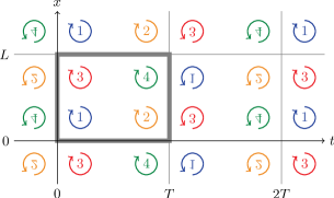
Figure 1: Illustration of the $P$-periodic boundary condition in the $t$ direction. The orientation changes when the boundary is crossed as indicated by the arrows. In the $x$ direction we have the usual periodicity. The base manifold is the rectangle with bold lines.

The straightforward way to define a global topological charge on a non-orientable manifold via the integral of a local topological charge density over the complete manifold, does not work: on a non-orientable manifold there is no global volume form to define integration. There is however a global volume element and one can define the integration of scalar densities like the action density. But one can not use this to also define the integration of a pseudo-scalar density over the full non-orientable manifold. As a workaround we define a total charge $Q_{m}$ on a maximal oriented submanifold

$$Q_{m}=\int_{0}^{T}\text{d}t\int\text{d}^{3}xq(x).$$ (2)

Here the integration is performed over the manifold with a cut at $t=0$, which makes the volume form well defined. This definition is the same as on open boundary lattices, but with an ad-hoc introduced cut without physical meaning. In the following we drop the index _m and define $Q:=Q_{m}$.

Then it is simple to show that on a non-orientable manifold this charge, defined as an integral of $q(x)$ over the base manifold, is not quantized. Under a parity transformation $P$ the topological charge transforms to its negative. Therefore applying a continuous translation on the gauge field in the time direction changes the charge continuously. After a translation of $T$ we get the same charge value, that we started with, but with an opposite sign. Since the charge varies continuously during the translation, it cannot possibly be quantized. Let us note, that the charge over the double cover, i.e. defined as an integral running from $0$ to $2T$ in time, is zero. However our setup is different from fixing the topology of a $L^{3}\times 2T$ lattice. The constraint in a fixed topology simulation is non-local, and leads to finite volume effects proportional to the inverse volume Brower et al. (2003). In contrast the $P$-periodic boundary condition gives a local quantum field theory by construction.

$P$ invariant quantities, like the gauge and fermion actions in QCD, are invariant under a translation in the $t$-direction. In contrast $P$ non-invariant observables change after such a translation, as we have seen already in the case of $q(x)$. To avoid large finite volume effects in $P$ non-invariant observables some care is necessary, see later. The translations in the $x,y,z$ directions and Euclidean rotations are not exact symmetries with the $P$-boundary condition. The violations of these symmetries originate from Feynman diagrams, where a particle propagates around the $t$-direction. Therefore they have to be exponentially suppressed with $T$ times the massgap of the theory.

The $P$-periodic boundary condition is similar to the $C$-periodic boundary condition of Refs. Wiese (1992); Kronfeld and Wiese (1991); Lucini et al. (2016), where a charge conjugation is performed when the boundary is crossed. They lead to processes, which change the total electric charge: charge fluctuations when propagating through the $C$-periodic boundary change their sign and thereby the total electric charge. Analogously our $P$-periodic boundary condition leads to changes in the total topological charge. Also, just as in the $C$-periodic case, the ultraviolet structure of the theory is not affected by the boundary condition and the same renormalization applies as in infinite volume Lucini et al. (2016).

The implementation of the parity transformation on parallel computers can be cumbersome. Therefore we choose another transformation, which serves the purpose equally well: the lattice points shall be reflected through the $x=0$ hyperplane. Since this transformation is a product of $P$ and a rotation by 180^∘ around the $x$-axis, it also changes the orientation and defines a non-orientable manifold. For simplicity we use the name “$P$-periodic” boundary condition for this setup in the rest of the paper.

Gauge fields

To demonstrate the viability of our proposal we performed numerical simulations in pure $\text{SU}(3)$ gauge theory. The prescription for the $P$-boundary is:

$$\begin{split}U_{x}(x,y,z,t+T)&=U^{\dagger}_{x}(L-x-1,y,z,t),\\ U_{i}(x,y,z,t+T)&=U_{i}(L-x,y,z,t)\end{split}$$ (3)

for $i=y,z,t$. In the other three directions we keep the usual periodic boundary condition. We use the tree level Symanzik improved action Luscher and Weisz (1985) and lattices of a fixed physical size of $L=T\sim 2.27/T_{c}$. One update sweep consists of four overrelaxation and one heatbath steps Cabibbo and Marinari (1982); Kennedy and Pendleton (1985); Creutz (1987). There is practically no overhead on the simulation time coming from the $P$-boundary condition. We chose five different lattice spacings. The lattice size, gauge coupling, $w_{0}$ scale Borsanyi et al. (2012), the lattice spacing, and the number of update sweeps are given in Table 1. The lattice spacings shown are obtained from the conversion $a=0.167\ \mathrm{fm}/w_{0}$ Sommer (2014). For comparison we simulate three streams at every set of parameters: one with periodic, one with open, and one with $P$-periodic boundaries. Our main observables are the topological charge $Q$ and time slice averages of the topological charge and action densities $Q(t)$ and $E(t)$ as defined in Luscher and Schaefer (2011). All are evaluated along the Wilson flow Lüscher (2010) at a flow time of $w_{0}^{2}$.

$L$	$\beta$	$w_{0}$	$a$[fm]	$n_{sweep}$
16	4.42466	1.79	0.093	$2\times 4001$
20	4.57857	2.24	0.075	$3\times 4001$
24	4.70965	2.65	0.063	$4\times 4001$
32	4.92555	3.43	0.049	$10\times 4001$
40	5.1	4.13	0.040	$19\times 4001$

Table 1: Lattice Parameters

Figure 2 shows the simulation time history of the topological charge for the finest lattice spacing. It already shows a drastic reduction of the autocorrelation of $Q$.

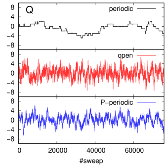
Figure 2: History of the topological charge $Q$ at $\beta=5.1$, the corresponding lattice spacing is $0.040$ fm.

The discrete nature of the topological charge in the periodic case can be seen best in a histogram of the topological charge, which is given in Figure 3 together with the histograms of the charges with the other two boundary conditions, which show no sign of discretization.

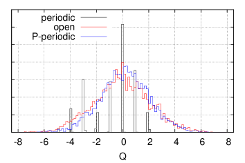
Figure 3: Histogram of the topological charge $Q$ at $\beta=5.1$, the corresponding lattice spacing is $0.040$ fm.

The lattice spacing dependence of the integrated autocorrelation time of the topological charge $\tau_{int}(Q)$ is given in Figure 4. Again one can clearly see that both open and $P$-periodic boundaries give a strong reduction of $\tau_{int}(Q)$ compared to the periodic case. Though $P$-periodic simulations have somewhat larger autocorrelation times than the open simulations, they seem to scale with a similar power of the lattice spacing.

In McGlynn and Mawhinney (2014b) a simple model was set up to describe the scaling of $\tau_{int}(Q)$ with the lattice spacing. There the autocorrelation function of the topological charge is investigated: $\Gamma(t,\tau)=\langle Q(t)_{\tau}Q(0)_{0}\rangle$, where $Q(t)_{\tau}$ is the time-slice topological charge after $\tau$ update sweeps. A diffusion equation for $\Gamma$ is set up, whose solutions describe numerical data from periodic and open lattices quite accurately. The extremely large autocorrelation times of the topological charge on periodic lattices are attributed to the presence of zero time-like momentum modes in $\Gamma$. They arise due to the periodicity of $\Gamma$ in the $t$-variable: $\Gamma(t+T,\tau)=\Gamma(t,\tau)$, which is the consequence of the periodic boundary $Q(t+T)=Q(t)$. These zero modes are shown to be eliminated by changing the boundary condition from periodic to open McGlynn and Mawhinney (2014b). Repeating the calculation for the $P$-boundary, we see that the same elimination occurs. The zero modes are absent since, as explained before, the charge is anti-periodic $Q(t+T)=-Q(t)$, and therefore $\Gamma$ is also anti-periodic: $\Gamma(t+T,\tau)=-\Gamma(t,\tau)$. Without these zero-modes the autocorrelation time of $Q$ scales similarly to that of the local observables. Let us note, that the diffusion and local tunneling parameters of this model do not depend on the boundary condition. Our findings are in agreement with the qualitative picture taken from this model calculation.

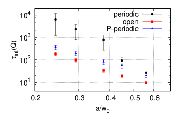
Figure 4: Integrated autocorrelation time of the topological charge as a function of the lattice spacing.

Now we come to the most important feature of our proposal. In contrast to the open boundary condition the $P$-periodic boundary is translationally invariant in the $t$-direction by construction. This is shown in Figures 5 and 6. Figure 5 gives the time-slice averaged action $E(t)$ as the function of time. For the usual and $P$-periodic boundaries $E(t)$ are practically constant and agree well with each other, reflecting translational symmetry and the absence of large finite volume effects. The open boundary result deviates from them significantly. Although it is expected to approach the periodic value in the middle of the lattice, here the time extent was not large enough to reach it.

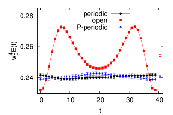
Figure 5: Time slice averaged action density at $\beta=5.1$, lattice spacing $a=0.040$ fm, and box size $1.6$ fm. Filled symbols give the per time slice results, while open symbols give the result for the full volume.

Similar effects can also be seen in Figure 6, which gives the integrated autocorrelation time of the topological charge on a time slice as a function of time. Again the results for periodic and $P$-periodic boundaries are independent of time, while the result for open boundaries has a dependence on the distance from the boundary. Additionally this plot shows that compared to the full volume results the integrated autocorrelation time of the topological charge on a single time slice improves for all choices of the boundary. In the periodic case, however, the result for a single time slice is larger than the result for open and $P$-periodic boundaries. The reasoning of the subvolume method Brower et al. (2014) would suggest that the autocorrelation time on the smallest subvolume – a single time slice – would be the same independent of the boundary conditions. In the diffusion model one can see why this might be not the case: there is a zero mode contributing to the autocorrelation time only in the periodic case, but not in the open or $P$-periodic case, which increases the autocorrelation.

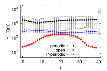
Figure 6: Integrated autocorrelation time of the topological charge on a time slice at $\beta=5.1$, lattice spacing $a=0.040$ fm, and box size $1.6$ fm. Filled symbols give the per time slice results, while open symbols give the result for the full volume.

The reason for $Q$ being not quantized with $P$-periodic boundary condition, is the lack of translational invariance for $Q$ as described earlier. This demands some additional care, when calculating an observable like the topological susceptibility. The appropriate procedure uses the definition via the topological charge density correlator, where we place the origin of the correlator to timeslice $T/2$:

$$\chi=\int_{0}^{T}\text{d}t\ \int\text{d}^{3}x\ \left\langle q(\vec{x},t)q(\vec{x},T/2)\right\rangle.$$ (4)

It has exponentially small finite volume corrections as $T$ is increased, since when $t$ in the integral is close to $0$ or $T$, the correlator is exponentially small. Also this definition is symmetric in $t$ and leads to a maximal cancellation of the negative tail of the correlator with its positive core. To illustrate this we generated dedicated ensembles at $\beta=4.42466$ with size $16^{3}\times T$ with $T=12,\dots 64$. The results show no significant finite volume effects, as shown in Figure 7 with label ’corr’. The more commonly used definition for the susceptibility is $\langle Q^{2}\rangle/(L^{3}T)$. For periodic boundary condition the two definitions are equivalent due to the translational invariance. In the $P$-periodic case the latter definition gives an observable, that has finite size effects proportional to $1/T$, see the points with label ’naive’ in Figure 7. Let us remark, that a similar prescription as in Equation 4 can also improve the finite volume correction of the standard subvolume method in periodic simulations.

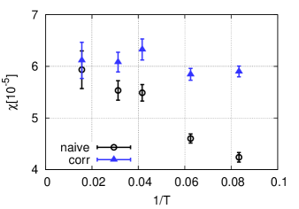
Figure 7: Finite size dependence of different topological susceptibility definitions for $P$-periodic boundary conditions at $\beta=4.42466$, lattice spacing $a=0.093$ fm.

Fermions

While non-orientability can be implemented on the gauge fields right away, it becomes non-trivial for fermions. As the boundary mixes the handedness it is not possible to define Weyl-fermions on a non-orientable manifold. The definition of Dirac-fermions is straightforward Grinstein and Rohm (1987), the fields undergo an $x$-axis reflection on the boundary. However we encounter a serious obstacle: the Dirac-matrix entering in the $x$-axis reflection ($\gamma_{5}\gamma_{x}$) spoils the $\gamma_{5}$-Hermiticity of the Dirac operator and leads to a complex fermion path integral. Numerical simulations with standard algorithms are not possible in this case. Here we show two workarounds.

The first solution is to combine the $x$-reflection with a charge conjugation. Since the topological charge is not only $P$-odd but also $CP$-odd, this combination has the same advantageous effect as the $P$-periodic boundary condition. Instead of the usual $\psi$, $\overline{\psi}$ fields, it turns out more convenient to work with the eigenstates of charge conjugation. These are the spinor fields $\eta_{a}$, $a=1,2$, defined in Lucini et al. (2016). In both bases we can write down the one flavor fermion action in infinite volume:

$$S_{f}=\overline{\psi}D[U]\psi=-\frac{1}{2}\eta_{a}C\hat{D}[U]_{ab}\eta_{b},$$ (5)

where $D$ is some possibly massive lattice Dirac-operator using the usual symmetric expression for the time derivatives, and $C$ is the charge conjugation matrix. The hatted Dirac-operator $\hat{D}[U]$ can be written with the original Dirac operator as $\hat{D}[U]_{ab}=D[\mathrm{Re}U\cdot\delta_{ab}-i\mathrm{Im}U\cdot\rho_{2,ab}]$ with the Pauli-matrices $\rho_{i}$ acting on the $a$-index of the $\eta_{a}$ fields. As the map $U\mapsto\mathrm{Re}U\cdot\delta_{ab}-i\mathrm{Im}U\cdot\rho_{2,ab}$ defines a representation of $\text{SU}(3)$ equivalent to $3\oplus 3^{\ast}$, Equation 5 is valid not only for Dirac operators which are linear in the links but also for operators which are linear in products of links, such as the clover improved Wilson Dirac operator. Equation 5 is even valid for some more general cases, like the overlap operator. For the readers convenience we collect the symmetries of $S_{f}$ in this somewhat uncommon representation in the Appendix. Now we introduce the “$CP$-boundary” condition:

$$\eta(x,y,z,t+T) =-\gamma_{5}\gamma_{x}\rho_{2}\rho_{3}\ \eta(L-x,y,z,t),$$ (6)

where we used the $x$-reflection and charge conjugation operators defined in the Appendix. The gauge fields also have to undergo a $CP$-transformation, this means additional complex conjugations in Equation (3). The resulting Dirac-operator is $\gamma_{5}\rho_{2}$-Hermitian

$$\hat{D}^{\dagger}=\gamma_{5}\rho_{2}\hat{D}\gamma_{5}\rho_{2},$$ (7)

since the matrix $\gamma_{5}\rho_{2}$ commutes with the boundary condition Metlitski (2015). Therefore the path integral over the $\eta$ fields gives a real Pfaffian. In the massless case and in the continuum $\hat{D}$ also satisfies

$$\{\hat{D},\gamma_{5}\rho_{2}\}=0\quad\quad\text{for}\quad m=0.$$ (8)

There is no continuous chiral symmetry behind this relation, but only a discrete one $\eta\to\gamma_{5}\rho_{2}\eta$. For further fermionic symmetries see the Appendix. The argument presented in Lucini et al. (2016) for the case of the $C$-boundary condition also applies for the $CP$-boundary: for those symmetries that are broken by the boundary, the breaking is expected to fall off exponentially in $T$.

Another solution to the complex determinant problem can be given for two degenerate flavors. Then the recipe is to add an extra rotation in flavor space at the boundary as

$$\eta(x,y,z,t+T) =-\gamma_{5}\gamma_{x}\rho_{2}\tau_{1}\ \eta(L-x,y,z,t),$$ (9)

where $\tau_{i}$’s are Pauli-matrices in flavor space, and now the $\eta$ carries a flavor index, too. This makes the fermion path integral real, since the Dirac-operator is $\gamma_{5}\tau_{3}$-Hermitian. This solution can be written in the usual four-component spinor basis, and it can be implemented in a similar way as the so-called $G$-parity boundary condition Bai et al. (2015). Equation 9 can be also applied to unrooted staggered fermions.

To get the expression for the two point pion correlation function, the interpolating operators are needed in the Majorana basis:

$$\begin{split}\mathcal{O}_{\pi^{-}}&=\overline{\psi}_{u}\gamma_{5}\psi_{d}=-\frac{1}{2}\eta_{u}^{T}\gamma_{5}C\left(1-\rho_{2}\right)\eta_{d}\\ \overline{\mathcal{O}}_{\pi^{-}}&=-\overline{\psi}_{d}\gamma_{5}\psi_{u}=\frac{1}{2}\eta_{d}^{T}\gamma_{5}C\left(1-\rho_{2}\right)\eta_{u}.\end{split}$$ (10)

The correlator between $x$ and $y$ then is

$$\left\langle\mathcal{O}_{\pi^{-}}(x)\,\overline{\mathcal{O}}_{\pi^{-}}(y)\right\rangle=-\frac{1}{4}\left\langle\big{(}\eta_{u}^{T})_{x}\gamma_{5}C\left(1-\rho_{2}\right)\big{(}\eta_{d}\big{)}_{x}\big{(}\eta_{d}^{T}\big{)}_{y}\gamma_{5}C\left(1-\rho_{2}\right)\big{(}\eta_{u}\big{)}_{y}\right\rangle,$$ (11)

which after integrating out the Grassmann fields and choosing $m_{u}=m_{d}$ becomes

$$\left\langle\mathcal{O}_{\pi^{-}}(x)\,\overline{\mathcal{O}}_{\pi^{-}}(y)\right\rangle=\frac{1}{4}\mathsf{Tr}\left[\big{(}\hat{D}^{-1}\big{)}_{y,x}\,\rho_{2}\,\big{(}\hat{D}^{-1}\big{)}^{\dagger}_{x,y}\,\rho_{2}+\big{(}\hat{D}^{-1}\big{)}_{y,x}\,\big{(}\hat{D}^{-1}\big{)}^{\dagger}_{x,y}\right].$$ (12)

More point correlations functions can be constructed analogously.

As a first exploratory study we implemented the $CP$-boundary condition with a Wilson-Dirac operator. Quenched configurations were generated with $CP$-boundary and we found, that the observables and in particular their autocorrelation times were consistent with the respective $P$-boundary condition values. To study the above proposal for fermions, we took $CP$-boundary configurations generated at $\beta=4.35$ on $16^{3}\times 32$ lattices, $w_{0}=1.57$. Four steps of stout smearing with smearing parameter $0.125$ were applied Morningstar and Peardon (2004). The $\pi^{+}$ pion propagator was measured at the bare Wilson-mass $-0.16$, see upper panel of Figure 8. Contrary to the usual periodic case the propagator is a single exponential for times far away from $t=0$ and $T$. There is no backward contribution coming from the anti-particle $\pi^{-}$. The reason for this is, that the anti-particle $\pi^{-}$ is now transformed under $CP$ conjugation to a $-\pi^{+}$. The corresponding propagation amplitude will be zero, since the matrix element of the pion annihilating operator between the $\pi^{+}$ and vacuum states is zero. To demonstrate the translational invariance, we also show fitted pion masses, that were obtained after shifting the gauge configuration in $t$-direction by 0, 8, 16, and 24 slices. The mass values are compatible with each other and also with the mass obtained from a lattice of same size with periodic boundary condition.

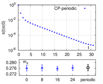
Figure 8: Upper: Pion propagator with $CP$-boundary condition. Lower: Pion masses obtained after shifting the gauge field by 0, 8, 16, and 24 units in t-direction (filled), and with periodic boundary condition (open).

Discussion and Outlook

The last sections show that a lot of properties of observables in the $P$-periodic setting are similar to or better than those in the open setting where the field space is connected. In particular the autocorrelation time of local quantities like the topological charge on a time slice improves to the level of open boundary conditions without showing boundary artefacts. But this does not mean that the field space in the $P$-periodic setup is connected. This can be seen for example in the instanton picture. In the periodic case the topological sectors are labeled by the net number of instantons with positive and negative charge $N_{+}-N_{-}$, which is an integer and conserved. The total instanton number $N_{+}+N_{-}$ is only conserved $\pmod{2}$ due to instanton pair creation and annihilation. For open lattices $N_{+}$, $N_{-}$, and $N_{+}\pm N_{-}$ are not well defined, so instantons do not lead to multiple sectors in field space. For the $P$-periodic case instantons can propagate once around the $P$-periodic direction and become anti-instantons, so $N_{+}$, $N_{-}$, and $N_{+}-N_{-}$ are also not well defined. But the total instanton number $N_{+}+N_{-}$ is conserved by this process and like on the torus well defined $\pmod{2}$. This suggests there are still two sectors in field space which correspond to the even and odd sectors on the torus, and that the same lattice artefacts are necessary to move between these sectors. Then also the critical slowing down affects the tunneling rate identically as on the torus. But in the case with $P$-periodic boundary conditions, i.e. only two sectors, it is much simpler to simulate long enough such that all sectors are sampled well. Already this makes the simulation at smaller lattice spacings feasible.

Having only two sectors also opens up possibilities to study even smaller lattice spacings with completely frozen topology if the relative weight of the two sectors is known. This can be achieved for example by integrating up the relative weight of the two sectors starting at a coupling where there is still enough tunneling between the sectors. This strategy has recently been applied at high temperatures where there are only two sectors relevant as well.Borsanyi et al. (2016); Frison et al. (2016) $P$-periodic boundaries make this method applicable also at low temperatures where on the torus at reasonable volumes many sectors with different relative weights contribute.

In this article we have shown how to formulate and simulate lattice QCD on a non-orientable space-time manifold. For the pure gauge case our simulations show that this change in the topology of space-time leads to a strong reduction of the autocorrelation time of the topological charge density comparable to the improvement observed using open boundary conditions. While the pure gauge case is straightforward to construct and its implementation is virtually free of additional numerical cost, the inclusion of fermions is not trivial. We have demonstrated how to combine non-orientable space-time with charge conjugation or flavor symmetry to get a real fermionic contribution to the action and also how to measure fermionic observables. Testing the new boundaries for dynamical fermions is left for future work. It will be especially interesting to compare the numerical costs to that of eg. open boundary conditions. Since it depends on the implementation details of fermions in the Majorana basis, we refrain from a precise cost estimation at this point.

Appendix

In this Appendix we list the symmetries of the single flavor fermion action in the Majorana representation, i.e. in the basis of eigenstates of the charge conjugation operation. For the definition see Lucini et al. (2016). We use the following representation for the charge conjugation matrix: $C=i\gamma_{y}\gamma_{t}=C^{\dagger}=C^{-1}=-C^{t}$. The usual fermion action is

$$S_{f}[\psi,\overline{\psi},U]=\overline{\psi}D[U]\psi.$$

Applying the following transformation

$$\eta=\frac{1}{\sqrt{2}}\begin{pmatrix}1&C\\ -i&iC\end{pmatrix}\begin{pmatrix}\psi\\ \overline{\psi}^{t}\end{pmatrix},$$

we get

$$S_{f}[\eta,U]=-\frac{1}{2}\eta^{t}C\hat{D}[U]\eta,$$

where $\hat{D}[U]=D[\mathrm{Re}U\cdot 1_{2\times 2}-i\mathrm{Im}U\cdot\rho_{2}]$.

.1 Infinite volume

First we start with the symmetries of the fermion action in infinite volume. The symmetries also apply in a finite box with periodic boundary conditions. The transformation for the gauge fields is standard and not shown explicitly.

1. U(1) phase transformation:

   $$\psi\to\exp(i\theta)\psi\quad\text{ and }\quad\overline{\psi}\to\overline{\psi}\exp(-i\theta),$$

   $$\eta\to\exp(-i\theta\rho_{2})\eta.$$

2. U(1) chiral transformation for a massless fermion in the continuum:

   $$\psi\to\exp(i\theta\gamma_{5})\psi\quad\text{ and }\quad\overline{\psi}\to\overline{\psi}\exp(i\theta\gamma_{5}),$$

   $$\eta\to\exp(i\theta\gamma_{5})\eta.$$

3. Charge conjugation:

   $$\psi\to C\overline{\psi}^{t}\quad\text{ and }\quad\overline{\psi}\to-\psi^{t}C,$$

   $$\eta\to\rho_{3}\eta.$$

4. Translations along the $\mu$-axis with $x^{\prime}_{\mu}=x_{\mu}+1$:

   $$\psi(x)\to\psi(x^{\prime})\quad\text{ and }\quad\overline{\psi}(x)\to\overline{\psi}(x^{\prime}),$$

   $$\eta(x)\to\eta(x^{\prime}).$$

5. $\mu$-axis reversal with $x^{\prime}_{\mu}=-x_{\mu}$:

   $$\psi(x)\to\gamma_{5}\gamma_{\mu}\psi(x^{\prime})\quad\text{ and }\quad\overline{\psi}(x)\to\overline{\psi}(x^{\prime})\gamma_{\mu}\gamma_{5},$$

   $$\eta(x)\to-\gamma_{5}\gamma_{\mu}\rho_{2}\eta(x^{\prime}).$$

6. 90^∘-rotation in $\mu\nu$-plane with $x^{\prime}_{\mu}=-x_{\nu},x^{\prime}_{\nu}=x_{\mu}$:

   $$\psi(x)\to\exp\!\left(-i\frac{\pi}{2}\sigma_{\mu\nu}\right)\psi(x^{\prime})\quad\text{ and }\quad\overline{\psi}(x)\to\overline{\psi}(x^{\prime})\exp\!\left(i\frac{\pi}{2}\sigma_{\mu\nu}\right),$$

   $$\eta(x)\to\exp\!\left(-i\frac{\pi}{2}\sigma_{\mu\nu}\right)\eta(x^{\prime}),$$

   where $\sigma_{\mu\nu}=-\frac{i}{4}\left[\gamma_{\mu},\gamma_{\nu}\right]$.

.2 $CP$-boundary

Here we list the symmetries of the theory with $CP$-boundary conditions. In the spatial directions we have usual periodic boundary conditions, whereas in the time direction we have

$$U_{x}(x,y,z,t+T) =U^{t}_{x}(L-x-1,y,z,t),$$

$$U_{i}(x,y,z,t+T) =U^{*}_{i}(L-x,y,z,t),\quad i=y,z,t$$

for the gauge fields and

$$\eta(x,y,z,t+T)=-\gamma_{5}\gamma_{x}\rho_{2}\rho_{3}\ \eta(L-x,y,z,t)$$

for the fermions. The symmetries are:

1. Sign transformation:

   $$\psi\to-\psi\quad\text{ and }\quad\overline{\psi}\to-\overline{\psi},$$

   $$\eta\to-\eta.$$

2. Combined chiral and $U(1)$ phase transformation for a massless fermion in the continuum:

   $$\psi\to-\gamma_{5}\psi\quad\text{ and }\quad\overline{\psi}\to\overline{\psi}\gamma_{5},$$

   $$\eta\to\gamma_{5}\rho_{2}\eta.$$

3. Charge conjugation combined with a $U(1)$ phase transformation:

   $$\psi\to iC\overline{\psi}^{t}\quad\text{ and }\quad\overline{\psi}\to i\psi^{t}C,$$

   $$\eta\to-i\rho_{2}\rho_{3}\eta.$$

4. Translations along the $\mu$-axis for $\mu=y,z,t$.

5. $\mu$-axis reversal for $\mu=y,z,t$.

   $\mu$-axis reversal combined with a $U(1)$ phase transformation for $\mu=x$:

   $$\psi(x)\to i\gamma_{5}\gamma_{\mu}\psi(x^{\prime})\quad\text{ and }\quad\overline{\psi}(x)\to-i\overline{\psi}(x^{\prime})\gamma_{\mu}\gamma_{5},$$

   $$\eta(x)\to i\gamma_{5}\gamma_{\mu}\eta(x^{\prime}).$$

6. 90^∘-rotation in the $yz$ plane.

References

- van Baal (1982) P. van Baal, Commun. Math. Phys. 85, 529 (1982).
- Schaefer et al. (2011) S. Schaefer, R. Sommer, and F. Virotta (ALPHA), Nucl. Phys. B845, 93 (2011), arXiv:1009.5228 [hep-lat] .
- Brower et al. (2014) R. Brower et al. (LSD), Phys.Rev. D90, 014503 (2014), arXiv:1403.2761 [hep-lat] .
- Luscher and Schaefer (2011) M. Luscher and S. Schaefer, JHEP 1107, 036 (2011), arXiv:1105.4749 [hep-lat] .
- Luscher and Schaefer (2013) M. Luscher and S. Schaefer, Comput. Phys. Commun. 184, 519 (2013), arXiv:1206.2809 [hep-lat] .
- Bruno et al. (2014) M. Bruno, P. Korcyl, T. Korzec, S. Lottini, and S. Schaefer, Proceedings, 32nd International Symposium on Lattice Field Theory (Lattice 2014), PoS LATTICE2014, 089 (2014), arXiv:1411.5207 [hep-lat] .
- Amato et al. (2015) A. Amato, G. Bali, and B. Lucini, in Proceedings, 33rd International Symposium on Lattice Field Theory (Lattice 2015) (2015) arXiv:1512.00806 [hep-lat] .
- Lucini et al. (2015) B. Lucini, C. McNeile, and A. Rago, in Proceedings, 33rd International Symposium on Lattice Field Theory (Lattice 2015) (2015) arXiv:1511.09303 [hep-lat] .
- Aoki et al. (2007) S. Aoki, H. Fukaya, S. Hashimoto, and T. Onogi, Phys. Rev. D76, 054508 (2007), arXiv:0707.0396 [hep-lat] .
- Bietenholz et al. (2015) W. Bietenholz, P. de Forcrand, and U. Gerber, JHEP 12, 070 (2015), arXiv:1509.06433 [hep-lat] .
- Bautista et al. (2015) I. Bautista, W. Bietenholz, A. Dromard, U. Gerber, L. Gonglach, C. P. Hofmann, H. Mejía-Díaz, and M. Wagner, Phys. Rev. D92, 114510 (2015), arXiv:1503.06853 [hep-lat] .
- Brower et al. (2003) R. Brower, S. Chandrasekharan, J. W. Negele, and U. J. Wiese, Phys. Lett. B560, 64 (2003), arXiv:hep-lat/0302005 [hep-lat] .
- Kitano and Yamada (2015) R. Kitano and N. Yamada, JHEP 10, 136 (2015), arXiv:1506.00370 [hep-ph] .
- Laio et al. (2015) A. Laio, G. Martinelli, and F. Sanfilippo, (2015), arXiv:1508.07270 [hep-lat] .
- McGlynn and Mawhinney (2014a) G. McGlynn and R. D. Mawhinney, Proceedings, 31st International Symposium on Lattice Field Theory (Lattice 2013): Mainz, Germany, July 29-August 3, 2013, PoS Lattice2013, 027 (2014a), arXiv:1311.3695 [hep-lat] .
- Endres et al. (2015) M. G. Endres, R. C. Brower, W. Detmold, K. Orginos, and A. V. Pochinsky, Phys. Rev. D92, 114516 (2015), arXiv:1510.04675 [hep-lat] .
- Detmold and Endres (2016) W. Detmold and M. G. Endres, (2016), arXiv:1605.09650 [hep-lat] .
- Wiese (1992) U. Wiese, Nucl.Phys. B375, 45 (1992).
- Kronfeld and Wiese (1991) A. S. Kronfeld and U. J. Wiese, Nucl. Phys. B357, 521 (1991).
- Lucini et al. (2016) B. Lucini, A. Patella, A. Ramos, and N. Tantalo, JHEP 02, 076 (2016), arXiv:1509.01636 [hep-th] .
- Luscher and Weisz (1985) M. Luscher and P. Weisz, Phys. Lett. B158, 250 (1985).
- Cabibbo and Marinari (1982) N. Cabibbo and E. Marinari, Phys. Lett. B119, 387 (1982).
- Kennedy and Pendleton (1985) A. D. Kennedy and B. J. Pendleton, Phys. Lett. B156, 393 (1985).
- Creutz (1987) M. Creutz, Phys. Rev. D36, 515 (1987).
- Borsanyi et al. (2012) S. Borsanyi, S. Durr, Z. Fodor, C. Hoelbling, S. D. Katz, et al., JHEP 1209, 010 (2012), arXiv:1203.4469 [hep-lat] .
- Sommer (2014) R. Sommer, Proceedings, 31st International Symposium on Lattice Field Theory (Lattice 2013), PoS LATTICE2013, 015 (2014), arXiv:1401.3270 [hep-lat] .
- Lüscher (2010) M. Lüscher, JHEP 08, 071 (2010), [Erratum: JHEP03,092(2014)], arXiv:1006.4518 [hep-lat] .
- McGlynn and Mawhinney (2014b) G. McGlynn and R. D. Mawhinney, Phys. Rev. D90, 074502 (2014b), arXiv:1406.4551 [hep-lat] .
- Grinstein and Rohm (1987) B. Grinstein and R. Rohm, Commun.Math.Phys. 111, 667 (1987).
- Metlitski (2015) M. A. Metlitski, (2015), arXiv:1510.05663 [hep-th] .
- Bai et al. (2015) Z. Bai et al. (RBC, UKQCD), Phys. Rev. Lett. 115, 212001 (2015), arXiv:1505.07863 [hep-lat] .
- Morningstar and Peardon (2004) C. Morningstar and M. J. Peardon, Phys. Rev. D69, 054501 (2004), arXiv:hep-lat/0311018 [hep-lat] .
- Borsanyi et al. (2016) S. Borsanyi et al., Nature 539, 69 (2016), arXiv:1606.07494 [hep-lat] .
- Frison et al. (2016) J. Frison, R. Kitano, H. Matsufuru, S. Mori, and N. Yamada, JHEP 09, 021 (2016), arXiv:1606.07175 [hep-lat] .