Abstract

The motivations of the $1/N$ expansion method in quantum field theory are explained. The method is first illustrated with the $O(N)$ model of scalar fields. A second example is considered with the two-dimensional Gross-Neveu model of fermion fields with global $U(N)$ and discrete chiral symmetries. The case of QCD is briefly sketched.

PACS numbers: 01.30.Bb, 11.10.Gh, 11.10.Hi, 11.15.Pg, 11.30.Hv, 11.30.Qc, 12.38.Aw.

Keywords: Large number of components, Global symmetries, Spontaneous symmetry breaking, Asymptotic freedom, Dynamical mass generation, Mass transmutation.

1 Introduction and motivations

Methods of resolution of quantum field theory equations are very rare. Usually one uses perturbation theory with respect to the coupling constant $g$, starting from free field theory. The size of (the dimensionless) $g$ gives an estimate of the strength of the interaction. The presence in the theory of other parameters than the coupling constant may allow the use of perturbation theory with respect to those parameters. This may enlarge the possibilities of approximate resolution of the theory.

A new parameter may emerge if the system under consideration satisfies symmetry properties with respect to a group of internal transformations. For example, constituents of the system (particles, nucleons, nuclei, energy excitations, etc.) belonging to different species, may have the same mass and possess the same dynamical properties with respect to the interaction. In such a case interchanges between these constituents would not modify the physical properties of the system. One might also consider transformations in infinitesimal or continuous forms, as in the case of the rotations in ordinary space. The system then satisfies an invariance property under continuous symmetry transformations. In many cases, the invariance might also be only approximate.

Among the continuous symmetry groups, two play an important role in physical problems. The first is $O(N)$, the orthogonal group, generated by the $N\times N$ orthogonal matrices. It has $N(N-1)/2$ parameters and generators. The second is $SU(N)$, the unitary group, generated by the $N\times N$ unitary complex matrices, with determinant equal to 1. It has $(N^{2}-1)$ parameters and generators.

In particle and nuclear physics, one has the approximate isospin symmetry group $SU(2)$ and the approximate flavor symmetry group $SU(3)$. Using these approximations, one can establish relations between masses and physical parameters of various particles, prior to solving the dynamics of the system under consideration.

In the cases of the groups $O(N)$ and $SU(N)$ mentioned above, $N$ has a well defined fixed value in each physical problem, $N=2,3,\ldots,$ etc. It is however tempting to consider the case where $N$ is a free parameter which can be varied at will. In particular, large values of $N$, with the limit $N\rightarrow\infty$, seem to be of interest. At first sight, it might seem that taking large values of $N$ would lead to more complicated situations, since the number of parameters increases and the group representations become intricate. However, it has been noticed that when the limit is taken in an appropriate way, in conjunction with the coupling constant of the theory, it may lead to simpler results than the cases of finite $N$. If this happens, then an interesting perspective of resolution is opened.

One may solve the problem in the simplified situation of the limit $N\rightarrow\infty$ and then, to improve the predictions, consider the contributions of the terms of order $1/N$ as a perturbation. If the true $N$ of the physical problem is sufficiently large, then the zeroth-order calculation done in the limit $N\rightarrow\infty$ would already provide the main dominant aspects of the solution of the physical problem under consideration. This is the spirit of the $1/N$ expansion method in quantum field theory. We emphasize that generally the solution thus obtained contains nonperturbative effects when expressed in terms of the coupling constant $g$ of the theory and therefore it provides nontrivial insight into the dynamics of the theory, which otherwise would be unattainable with the use of ordinary perturbation theory with respect to $g$.

The interest of the large-$N$ limit was first noticed by Stanley [1] in statistical physics, who used it in the framework of the Heisenberg model (spin-spin interactions). He showed that in that limit the model reduces to the spherical approximation of the Ising model, which was soluble.

The method was introduced in quantum field theory by Wilson [2], who applied it to the $O(N)$ model of scalar fields and to the $U(N)$ model of fermion fields.

In 1974, ’t Hooft [3, 4] applied it to Quantum Chromodynamics (QCD), the newly born theory of the strong interaction, which is a gauge theory with the non-Abelian gauge group $SU(3)_{c}$ in the internal space of color quantum numbers. (Not to be confused with the global flavor symmetry group $SU(3)$ met previously.) This theory cannot be solved with the only large-$N$ limit, but many simplifications occur there. In two space-time dimensions, it is almost soluble.

We shall illustrate the method by two explicit examples: 1) The $O(N)$ model of scalar fields; 2) The two-dimensional model of Gross and Neveu with global $U(N)$ symmetry of fermion fields and discrete chiral symmetry.

Reviews and lectures on the $1/N$ expansion method can be found in Refs. [5, 6, 7, 8] (the list is not exhaustive).

2 The scalar $\mathbf{O(N)}$ model

The $O(N)$ model is a theory of $N$ real scalar fields $\phi^{a}$ ($a=1,2,\ldots,N$), with a quartic interaction, invariant under the $O(N)$ group of transformations. This group is similar in structure to the rotation group, but acts in the internal space of $N$ species of the fields.

The Lagrangian density is (in units where $\hbar=c=1$)

$$\mathcal{L}=\frac{1}{2}\ \partial_{\mu}\phi^{a}\partial^{\mu}\phi^{a}-\frac{1}{2}\ \mu_{0}^{2}\phi^{a}\phi^{a}-\frac{\lambda_{0}}{8N}(\phi^{a}\phi^{a})^{2}.$$ (1)

(Summation on repeated indices is understood. $\partial_{\mu}=\frac{\partial}{\partial x^{\mu}}$, etc.) $\mu_{0}^{2}$ and $\lambda_{0}$ are real parameters, representing the bare mass squared and the bare coupling constant; the physical mass and coupling constant could be defined only after quantum radiative corrections are taken into account. In four space-time dimensions the coupling constant is dimensionless. The factor $1/N$ has been explicitly introduced in the interaction term for future convenience. When the limit $N\rightarrow\infty$ is taken, the coupling constant $\lambda_{0}$ will be assumed to be independent of $N$. Had we defined a coupling constant $\tilde{\lambda}_{0}$ as being equal to $\lambda_{0}/N$, we would be obliged later, to maintain a physical content for the theory, to assume that the product $N\tilde{\lambda}_{0}$ remains finite in the above limit, which leads back to our initial choice.

A detailed study of this model can be found in Ref. [9].

2.1 Classical approximation

We search for the ground state of the theory at the classical level. The lagrangian density is composed of the kinetic energy density minus the potential energy density. The kinetic energy term gives generally a positive contribution to the total energy of the system. Its minimum value is zero, corresponding to constant fields. We stick to that situation. The potential energy density is then

$$U=\frac{1}{2}\ \mu_{0}^{2}\phi^{a}\phi^{a}+\frac{\lambda_{0}}{8N}(\phi^{a}\phi^{a})^{2}.$$ (2)

This is a quartic function of the $\phi$s. It is evident that the energy is not bounded from below if $\lambda_{0}<0$. In this case there is no a stable ground state. We assume henceforth that $\lambda_{0}>0$.

Two cases have to be distinguished: 1) $\mu^{2}_{0}>0$; 2) $\mu^{2}_{0}<0$.

1) $\mu^{2}_{0}>0$.

The shape of the function $U$ is presented in Fig. 1.

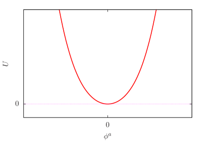
Figure 1: The potential energy density for $\mu^{2}_{0}>0$.

The minimum of the energy corresponds to the values $\phi_{0}^{a}=0,\ (a=1,\ldots,N)$. The $\phi$s in this case can be considered as excitations from the ground state.

Considering the lagrangian density (1), we can interpret it as describing the dynamics of $N$ particles with degenerate masses, equal to $\mu_{0}$, interacting by means of the quartic interaction. We have complete $O(N)$ symmetry between the particles.

This mode of symmetry realization is called the Wigner mode or the normal mode.

2) $\mu^{2}_{0}<0$.

The shape of the function $U$ is presented in Fig. 2.

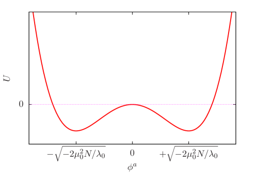
Figure 2: The potential energy density for $\mu^{2}_{0}<0$.

The minimum of the energy is no longer $\phi_{0}^{a}=0$, but a shifted value at $\phi_{0}^{a}=\pm\sqrt{-\frac{2\mu_{0}^{2}N}{\lambda_{0}}}\equiv<\phi>$ for one of the $a$ s. There is a degeneracy between the different $\phi^{a}$s. For definiteness, we choose the ground state at the minimum obtained with $\phi^{N}$.

We redefine the fields around the new ground state:

$$\chi=\phi^{N}-<\phi>,\ \ \ \ \ \ \ \pi^{a}=\phi^{a},\ \ \ a=1,\ldots,N-1.$$ (3)

The potential energy density becomes

$$U=-\mu_{0}^{2}\chi^{2}+\frac{\lambda_{0}}{2N}<\phi>\chi^{3}+\frac{\lambda_{0}}{8N}(\pi^{a}\pi^{a}+\chi^{2})^{2}.$$ (4)

The fields $\pi^{a}$ have no longer mass terms, while the field $\chi$ has a mass term. We have now the masses:

$$m_{\pi^{a}}^{2}=0,\ \ \ \ a=1,\ldots,N-1,\ \ \ \ \ \ m_{\chi}^{2}=-2\mu_{0}^{2}.$$ (5)

The $O(N)$ symmetry that we had initially has partially disappeared. There is now $O(N-1)$ symmetry in the space of the fields $\pi^{a}$. It is said that the $O(N)$ symmetry has been spontaneously broken. This happened because the ground state of the theory is not symmetric, while the lagrangian density is.

This phenomenon is accompanied with the appearance of $(N-1)$ massless fields. These are called Goldstone bosons. This way of realization of the symmetry is called the Goldstone mode.

In particle and nuclear physics, the isospin $SU(2)$ symmetry and the quark flavor $SU(3)$ symmetry are realized with the Wigner mode. The chiral $SU(3)_{R}\times SU(3)_{L}$ symmetry is realized with the Goldstone mode.

2.2 Quantum effects

We want now to take into account the quantum effects of the model that we are considering. For this, it is necessary to compute the quantum corrections that contribute to the potential energy. In quantum field theory, these are represented by the radiative corrections.

The definition of the potential energy density $U$ is enlarged. The new potential energy is called the effective potential, which is composed of the classical part, $U_{\mathrm{class}}$, that we met before [Eq. (2)], and of a part, $U_{\mathrm{rad}}$, coming from the radiative corrections:

$$U_{\mathrm{eff}}=U_{\mathrm{class}}+U_{\mathrm{rad}}\ .$$ (6)

$U_{\mathrm{rad}}$ is best defined in the path integral formalism. We refer the reader to Ref. [10] and to the many textbooks that exist on the subject. The key object is the generating functional of one-particle irreducible diagrams or proper vertices. The effective potential is obtained from the latter by considering only external constant fields in $x$-space or external lines with zero momenta in momentum space. Diagramatically, $U_{\mathrm{rad}}$ is given by the sum of all loop diagrams with such external lines. These are also accompanied with appropriate combinatorial factors due to the existing symmetry properties under exchanges among the external lines [11]. Another method of calculation hinges on a direct evaluation of the path integral contribution, avoiding explicit summation of diagrams, [12]. However, whatever the method of evaluation is, the exact calculation of the effective potential is almost impossible, since it involves an infinity of many complicated contributions. Nevertheless, the use of the $1/N$ expansion method considerably simplifies the situation. The leading terms of this expansion are calculable.

Prior to the evaluation of the effective potential, we shall introduce the propagators, vertices and loops, that are needed for our calculations.

2.3 Propagators, vertices and loops

The radiative corrections can be calculated starting from the situation where $\mu_{0}^{2}>0$. Radiative corrections will modify the value of $\mu_{0}^{2}$, bringing it into a new value $\mu^{2}$. It is then sufficient to consider at the end the analytic continuation of $\mu^{2}$ into negative values to complete the study. We therefore consider the initial Lagrangian density (1):

$$\mathcal{L}=\frac{1}{2}\ \partial_{\mu}\phi^{a}\partial^{\mu}\phi^{a}-\frac{1}{2}\ \mu_{0}^{2}\phi^{a}\phi^{a}-\frac{\lambda_{0}}{8N}(\phi^{a}\phi^{a})^{2}.$$ (7)

The inverse of the free propagator of the field $\phi^{a}$ is essentially represented by the coefficients of the quadratic parts of $\mathcal{L}$. In momentum space, the free propagator is

$$D_{0}^{ab}(p)=\delta_{ab}D_{0}(p)=\int d^{4}xe^{{\displaystyle ip.x}}<0|T(\phi^{a}(x)\phi^{b}(0))|0>,$$ (8)

where the last term represents the vacuum expectation value of the chronological product of the field operators, and $D_{0}$ has the expression

$$D_{0}(p)=\frac{i}{p^{2}-\mu_{0}^{2}+i\varepsilon}\hskip 28.45274pt\Longleftrightarrow\hskip 28.45274pt\begin{picture}(0.0,0.0)\includegraphics{f3-nexpm.pstex}\end{picture}\begin{picture}(2091.0,66.0)(2893.0,-4369.0)\end{picture}\ \ \ \ \ \ .$$ (9)

We have associated with the propagator a graphical representation in the form of a full straight line.

The bare vertex is equal to the coefficient of the four-field interaction term (contact interaction), with a multiplicative factor $i$ (Fig. 3). Its order in $N$, for large values of $N$, is $N^{-1}$.

Figure 3: The bare vertex. We have explicitly indicated its order in $N$.

Radiative corrections are represented by loops, made of closed lines (propagators). Figs. 4 and 5 represent examples of one-loop and two-loop diagrams, respectively. The order in $N$ of a loop diagram is calculated by taking into account that of the vertex at the contact point of the loop with the external lines and that of the possibly existing summation of indices of the loop. Thus, if the index $b$ of the propagators of a loop is independent of the index $a$ of external lines, then it is summed over the $N$ values the index $b$ can take; $b$ in this case is a dummy index; therefore it produces a multiplicative factor $N$. External lines are not counted.

Figure 4: Examples of one-loop diagrams with their order in $N$.

\begin{picture}(8931.0,8201.0)(1093.0,-8329.0)\end{picture}

Figure 5: Examples of two-loop diagrams.

2.4 The auxiliary field method

We observe on Fig. 4 that the last two diagrams, which have the same topological structure, have different behaviors for large $N$, depending on the values of indices the loop propagators have. This is an annoying situation, because at higher orders (many loops) it becomes more and more difficult to continue the analysis, since the number of possibilities the indices can have rapidly increases with a corresponding increase of different categories of behavior in $N$. The ideal situation is the one in which all diagrams with the same topological structure have the same behavior in $N$; in such a case, we do not need to consider the detailed values of indices of each line.

To remedy the present difficulty, we shall resort to a method, called the auxiliary field method, often used in quantum field theory, which consists of replacing composite fields by a new, nonpropagating field, without changing the physical content of the theory. The validity of the latter property is rather easily shown in the path integral formalism; when an operator formalism is used, a simple hint is provided with the use of the equations of motion.

We wish to replace the composite field $\phi^{a}\phi^{a}$ appearing in the interaction term by a single field, which we shall designate by $\sigma$. (Since in $\phi^{a}\phi^{a}$, $a$ is summed from one to $N$, this field does not have any index; it is a singlet under the $O(N)$ group of transformations.) To this end, we add to the Lagrangian density (7) a new term, thus defining a new Lagrangian density:

$$\mathcal{L^{\prime}}=\mathcal{L}+\frac{N}{2\lambda_{0}}\ \Big{(}\sigma-\frac{\lambda_{0}}{2N}\ \phi^{a}\phi^{a}-\mu_{0}^{2}\Big{)}^{2}.$$ (10)

The $\sigma$ field does not have kinetic energy. The terms in the added expression are chosen such that the quartic term in $\phi$ as well as the mass term of $\phi$ disappear from the new Lagrangian density. The equation of motion (Euler-Lagrange equation) of $\sigma$ yields its definition:

$$\sigma=\frac{\lambda_{0}}{2N}\ \phi^{a}\phi^{a}+\mu_{0}^{2}.$$ (11)

The latter also shows that the added term in the lagrangian is zero if the equation of motion of $\sigma$ is used. One may conclude that the new lagrangian is equivalent to the former one:

$$\mathcal{L^{\prime}}\approx\mathcal{L}.$$ (12)

$\mathcal{L^{\prime}}$ takes the form:

$$\mathcal{L^{\prime}}=\frac{1}{2}\ \partial_{\mu}\phi^{a}\partial^{\mu}\phi^{a}+\frac{N}{2\lambda_{0}}\sigma^{2}-\frac{1}{2}\sigma\phi^{a}\phi^{a}-\frac{N\mu_{0}^{2}}{\lambda_{0}}\sigma.$$ (13)

We have now two types of field, the $\phi$s and $\sigma$, with an interaction term between them which is no longer quartic.

We reanalyze the properties of the propagators, the vertex and the loops with the new Lagrangian.

The bare propagators are

$$D_{0\phi}(p)=\frac{i}{p^{2}+i\varepsilon}\ \ \Longleftrightarrow\ \ \begin{picture}(0.0,0.0)\includegraphics{f3-nexpm.pstex}\end{picture}\begin{picture}(2091.0,66.0)(2893.0,-4369.0)\end{picture}\ \ \ =O(N^{0}),$$ (14)

$$D_{0\sigma}(p)=\frac{i\lambda_{0}}{N}\ \ \Longleftrightarrow\ \ \begin{picture}(0.0,0.0)\includegraphics{f7-nexpm.pstex}\end{picture}\begin{picture}(2406.0,66.0)(1588.0,-3739.0)\end{picture}\ \ \ =O(N^{-1}).$$ (15)

The bare vertex $\sigma\phi\phi$, with coefficient $-i/2$, is represented in Fig. 6.

Figure 6: The vertex $\sigma\phi\phi$ and its order in $N$.

Loops and higher-order diagrams are represented in Figs. 7 and 8.

Figure 7: Higher-order diagrams and their order in $N$.

Figure 8: Higher-order diagrams and their order in $N$.

In the analysis of the above diagrams external lines are not counted. We observe now many new properties with respect to the former situation of Sec. 2.3. First, because of the behavior of the $\sigma$ propagator as $O(N^{-1})$, every internal $\sigma$ line introduces an additional factor $N^{-1}$ in the behavior of the corresponding diagram. Therefore, diagrams containing an increasing number of internal $\sigma$ lines become nondominant. The leading diagrams in their behavior in $N$ will be those that contain the least possible number of internal $\sigma$ lines. Second, loops of $\phi$s can occur only if they are joined to $\sigma$ lines or propagators or within the latter. Multiloop diagrams of $\phi$s are of the type of the first diagram of Fig. 8 and of its generalizations. However, such diagrams, as well as the second diagram of Fig. 7, are not of the one-particle irreducible type, since by cutting one internal $\sigma$ propagator, the diagrams become separated into two disconnected diagrams. Therefore, they cannot enter into the definition of the effective potential. The only loop diagrams of $\phi$s to be considered are represented by the third diagram of Fig. 7 and the last two diagrams and their generalizations of Fig. 8. The latter, containing internal $\sigma$ lines, are nondominant with respect to the first one.

In conclusion, in the limit of large $N$, the leading loop contributions to the effective potential will come from the third type of diagram of Fig. 7 and of its generalizations, where one can have any number of external $\sigma$ lines (cf. Fig. 9).

2.5 Renormalization

The effective potential can now be calculated. As expressed in Eq. (6), it is composed of two parts, $U_{\mathrm{class}}$ and $U_{\mathrm{rad}}$, corresponding to the classical part and to the part receiving contributions of radiative corrections, respectively:

$$U_{\mathrm{eff}}=U_{\mathrm{class}}+U_{\mathrm{rad}}\ .$$ (16)

The classical part is fixed by the content of the Lagrangian density (13):

$$U_{\mathrm{class}}=-\frac{N}{2\lambda_{0}}\sigma^{2}+\frac{1}{2}\sigma\phi^{a}\phi^{a}+\frac{N\mu_{0}^{2}}{\lambda_{0}}\sigma.$$ (17)

The radiative corrections are given by the sum of $\phi$ loop diagrams with an increasing number of external $\sigma$ lines (Fig. 9). Here, according to the definition of the effective potential, the external $\sigma$ fields should be considered as constants in $x$-space, or, equivalently, carrying zero momenta in momentum space.

Figure 9: Diagrams contributing to the radiative corrections in the effective potential at leading order in $N$.

The summation of the above diagrams, with appropriate combinatorial factors, can be done with conventional methods [9, 11]. The loop calculation involves a four-dimensional integration in Minkowski space of $\phi$ propagators (14). Because of the presence of the additive factor $i\varepsilon$ in the denominator of the propagator, the latter has a well-defined analyticity property, which allows one to rotate the $k_{0}$-integration from the real axis to the imaginary axis and to calculate the integrals in Euclidean space. This amounts to replacing in the integrals $k_{0}$ with $ik_{4}$, with $k_{4}$ real. In the following, we shall write the integrals directly in Euclidean space, with the definition $k^{2}=\sum_{i=1}^{4}k_{i}^{2}>0$.

After summation of the diagrams, the effective potential takes the form

$$U_{\mathrm{eff}}=-\frac{N}{2\lambda_{0}}\sigma^{2}+\frac{1}{2}\sigma\phi^{a}\phi^{a}+\frac{N\mu_{0}^{2}}{\lambda_{0}}\sigma+\frac{N}{2}\int\frac{d^{4}k}{(2\pi)^{4}}\ln(k^{2}+\sigma).$$ (18)

We are interested by the stationary point of $U_{\mathrm{eff}}$ (ground state). We therefore calculate its partial derivatives with respect to $\sigma$ and $\phi^{a}$:

$$\frac{\partial U_{\mathrm{eff}}}{\partial\sigma}=-\frac{N}{\lambda_{0}}\sigma+\frac{1}{2}\phi^{a}\phi^{a}+\frac{N\mu_{0}^{2}}{\lambda_{0}}+\frac{N}{2}\int\frac{d^{4}k}{(2\pi)^{4}}\frac{1}{(k^{2}+\sigma)}\ ,$$ (19)

$$\frac{\partial U_{\mathrm{eff}}}{\partial\phi^{a}}=\phi^{a}\sigma,\ \ \ \ \ \ \ a=1,\ldots,N.$$ (20)

The integral that appears in Eq. (19) is divergent for values of $k\rightarrow\infty$. This is a general problem of quantum field theory, which reflects the singular behavior of the theory at high energies or at short distances between the fields in $x$-space. To cure this difficulty, one generally tries to absorb the divergent parts into the bare coupling constant and the mass, as well as into redefinitions of the fields, defining finite quantities. If this happens, then the theory is classified as being of the renormalizable type. However, not all theories satisfy this requirement. There might arise divergences, with specific structure, which could not be absorbed by existing quantities. As we shall see, the present theory is of the renormalizable type.

To study the possible renormalizability of the theory, we isolate in the integrand of the above integral the dominant parts of the asymptotic behavior:

$$\frac{1}{k^{2}+\sigma}_{\stackrel{{\scriptstyle{\displaystyle\rightarrow}}}{{k^{2}\rightarrow\infty}}}\ \frac{1}{k^{2}}-\frac{\sigma}{(k^{2})^{2}}+O(1/(k^{2})^{3}).$$ (21)

The first two terms lead to ultraviolet divergences by integration. We cannot, however, manipulate them as they stand, since the second term would lead to a new artificial infrared divergence (when $k\rightarrow 0$). We have to incorporate in the second term a mass factor in the denominator to render it softer in the infrared region.

We add and subtract in $\frac{\partial U_{\mathrm{eff}}}{\partial\sigma}$ the following quantities:

$$\frac{N}{2}\int\frac{d^{4}k}{(2\pi)^{4}}\frac{1}{k^{2}}-\frac{N}{2}\sigma\int\frac{d^{4}k}{(2\pi)^{4}}\frac{1}{k^{2}(k^{2}+M^{2})},$$ (22)

where $M$ is an arbitrary mass term.

The result is

$$\frac{\partial U_{eff}}{\partial\sigma} = -N\sigma\Big{(}\ \frac{1}{\lambda_{0}}+\frac{1}{2}\int\frac{d^{4}k}{(2\pi)^{4}}\frac{1}{k^{2}(k^{2}+M^{2})}\ \Big{)}+\frac{1}{2}\phi^{a}\phi^{a}$$ (23)

$$\ +N\Big{(}\ \frac{\mu_{0}^{2}}{\lambda_{0}}+\int\frac{d^{4}k}{(2\pi)^{4}}\frac{1}{k^{2}}\ \Big{)}+\frac{N}{32\pi^{2}}\sigma\ln(\frac{\sigma}{M^{2}}).$$

The infinite integrals, together with the bare coupling constant and the bare mass term, may define finite renormalized quantities. This would be possible if we admit that the bare quantities $\lambda_{0}$ and $\mu_{0}^{2}$ may eventually take unphysical values. We thus define a finite coupling constant $\lambda$ and a finite mass term $\mu^{2}$ with the equations

$$\frac{1}{\lambda(M)}=\frac{1}{\lambda_{0}}+\frac{1}{2}\int\frac{d^{4}k}{(2\pi)^{4}}\frac{1}{k^{2}(k^{2}+M^{2})},$$ (24)

$$\frac{\mu^{2}(M)}{\lambda(M)}=\frac{\mu_{0}^{2}}{\lambda_{0}}+\int\frac{d^{4}k}{(2\pi)^{4}}\frac{1}{k^{2}}.$$ (25)

The finite quantities depend on the arbitrary mass parameter $M$. For each fixed value of $M$, they take a corresponding value.

One can better study this dependence by comparing for instance the value of the coupling constant $\lambda(M)$ to a reference value $\lambda_{1}\equiv\lambda(M_{1})$ corresponding to a reference mass parameter $M_{1}$. One obtains from the comparison of the corresponding two equations:

$$\frac{1}{\lambda(M)}=\frac{1}{\lambda_{1}}-\frac{1}{32\pi^{2}}\ln(\frac{M^{2}}{M_{1}^{2}}).$$ (26)

This equation is called the renormalization group equation (RGE) and plays an important role for the analysis and understanding of the properties of the theory.

We can also express $\lambda(M)$ in terms of $\lambda_{1}$ and the other parameters:

$$\lambda(M)=\frac{\lambda_{1}}{1-\frac{\lambda_{1}}{32\pi^{2}}\ln(\frac{M^{2}}{M_{1}^{2}})}.$$ (27)

$\lambda_{1}$ and generally $\lambda(M)$ are assumed positive for physical reasons (below boundedness of the energy; see the discussion of the classical potential energy density after Eq. (2)). Therefore, we consider domains of solution where this condition is satisfied.

From the last equation we deduce that when $M$ increases starting from $M_{1}$, $\lambda(M)$ increases. When $M$ reaches the value $M_{\mathrm{cr}}=M_{1}\exp(16\pi^{2}/\lambda_{1})$, $\lambda(M)$ diverges and for larger values of $M$, $\lambda$ becomes negative. This is a sign of the instability of the theory for large values of $\lambda$.

The RGE can also be formulated in the form of a differential equation. Defining

$$M\frac{\partial\lambda(M)}{\partial M}=\beta(\lambda(M)),$$ (28)

one finds from the finite form of $\lambda(M)$ [Eq. (27)]

$$\beta(\lambda)=\frac{\lambda^{2}}{16\pi^{2}}>0,$$ (29)

which shows that $\lambda(M)$ is an increasing function of $M$.

What is the interest of the RGE? In perturbation theory, when calculating radiative corrections, one usually finds powers of the quantity $\lambda^{2}\ln(p^{2}/M^{2})$, where $p$ is a representative of the momenta of the external particles. Even if $\lambda$ is chosen small, at high energies, i.e., at large values of $p$, the logarithm may become large enough to invalidate perturbative calculations. However, since the logarithm depends on $M$ for dimensional reasons, one can choose the latter of the order of $p$ to maintain the logarithm small. This could be useful, if on the other hand $\lambda$ remains bounded or small at these values of $M$. The RGE precisely gives us the answer to that question, indicating the way $\lambda$ behaves at large values of $M$.

Coming back to our theory, we see from the previous results that this is not the case here: $\lambda$, on the contrary, increases with $M$ and diverges at $M_{\mathrm{cr}}$. The theory is ill-defined at high energies. In $x$-space, high energies correspond to short distances. The interaction becomes stronger when the distance between two sources or two particles decreases. A similar behavior is also found in Quantum Electrodynamics (QED). These theories are better defined at low energies or large distances.

Theories for which the coupling constant decreases at high energies or at short distances are called asymptotically free.

Summarizing the results of this section, we recall that we could get rid of the divergent parts of the integrals by absorbing them in the bare coupling constant and the bare mass term, redefining at the end a finite coupling constant and a finite mass term. The theory we are considering is therefore renormalizable. The price that is paid is the introduction of an arbitrary mass parameter that essentially fixes the mass scale of the physical quantities of the theory.

2.6 The ground state

Using Eqs. (24) and (25), one can express the effective potential and its derivatives [Eqs. (18), (19) and (20)] in terms of the finite coupling constant and mass term. To simplify the notation, we denote $\lambda(M)=\lambda$ and $\mu^{2}(M)=\mu^{2}$.

The effective potential is

$$U_{\mathrm{eff}}=\frac{1}{2}\phi^{a}\phi^{a}\sigma-\frac{N\sigma^{2}}{2\lambda}(1+\frac{\lambda}{64\pi^{2}})+\frac{N\mu^{2}\sigma}{\lambda}+\frac{N\sigma^{2}}{64\pi^{2}}\ln(\frac{\sigma}{M^{2}}).$$ (30)

The equations defining the minimum of the effective potential are

$$\frac{\partial U_{\mathrm{eff}}}{\partial\sigma}=-\frac{N\sigma_{0}}{\lambda}+\frac{1}{2}\phi_{0}^{a}\phi_{0}^{a}+\frac{N\mu^{2}}{\lambda}+\frac{N}{32\pi^{2}}\sigma_{0}\ln(\frac{\sigma_{0}}{M^{2}})=0,$$ (31)

$$\frac{\partial U_{eff}}{\partial\phi^{a}}=\phi_{0}^{a}\sigma_{0}=0,\ \ \ \ \ \ a=1,\ldots,N.$$ (32)

From Eqs. (32), one deduces two possibilities: 1) $\phi_{0}^{a}=0$; 2) $\sigma_{0}=0$.

1) $\phi_{0}^{a}=0$  ($a=1,\ldots,N$), $\sigma_{0}\neq 0$. From Eq. (31) one obtains

$$\sigma_{0}\Big{(}1-\frac{\lambda}{32\pi^{2}}\ln(\frac{\sigma_{0}}{M^{2}})\Big{)}=\mu^{2}.$$ (33)

The presence of the logarithm imposes $\sigma_{0}>0$. For small values of $\lambda$, one has $\mu^{2}>0$. By continuity to larger values, one should search for positive solutions of $\sigma_{0}$. Let $\sigma_{0}$ be the solution of the equation for a certain domain of $\lambda$ and $\mu^{2}$. One should redefine the field $\sigma$ from the value of $\sigma_{0}$:

$$\sigma(x)=\sigma^{\prime}(x)+\sigma_{0}.$$ (34)

The corresponding shift of $\sigma$ in the Lagrangian gives back a common mass to the fields $\phi^{a}$. We are in a situation where the $O(N)$ symmetry is realized in the Wigner mode.

2) $\sigma_{0}=0$. From Eq. (31) one obtains

$$\frac{1}{2}\phi_{0}^{a}\phi_{0}^{a}+\frac{N\mu^{2}}{\lambda}=0.\ \ \ \ \Longrightarrow\ \ \ \ \ \mu^{2}<0.$$ (35)

$$\phi_{0}^{a}\phi_{0}^{a}=-\frac{2N\mu^{2}}{\lambda}.$$ (36)

There is a degeneracy of solutions for the $\phi_{0}^{a}$s. One can choose for example:

$$\phi_{0}^{a}=0,\ \ \ \ a=1,\ldots,N-1,\ \ \ \ \ \ \phi_{0}^{N}=\sqrt{-\frac{2N\mu^{2}}{\lambda}}\equiv<\phi>.$$ (37)

One then develops $\phi^{N}$ around $<\phi>$:

$$\phi^{N}(x)=\chi(x)+<\phi>.$$ (38)

The symmetry is realized in the Goldstone mode, with the presence of $(N-1)$ massless fields $\phi^{a}$ and one massive field $\chi$.

We summarize the results obtained so far. The $O(N)$ model defines a renormalizable theory. The radiative corrections introduce limitations into the validity domain of the model. The coupling constant increases at high energies and diverges at some critical mass scale. The ground state equations also introduce new constraints on the parameters of the model. The two modes of realization of the symmetry, found at the classical level, remain valid within the restricted domain of the parameters. The above results are obtained at the leading-order of the $1/N$ expansion, which allows us to simplify in a consistent way the equations of the theory, to solve them and to have an insight on the dynamics, going beyond ordinary perturbation theory. Unfortunately, the $O(N)$ model is not a stable theory as a whole, and the continuation of the investigations at nonleading orders of the expansion in $1/N$ reveals new restrictions and instabilities.

3 The Gross-Neveu model

3.1 General properties

We consider now an analog of the $O(N)$ model with the boson fields replaced by fermion fields of $N$ different species with the same mass. Since Dirac fermion fields are not generally hermitian, the symmetry group of transformations that leaves the Lagrangian density invariant is $U(N)$. Theories with four-fermion interactions are not renormalizable in four space-time dimensions. This is related to the fact that the fermion fields have mass dimension 3/2, instead of 1 for the boson fields. The interaction term has thus dimension 6, greater than the dimension of the Lagrangian density which is 4 (dimensions of multiplicative coefficients are not considered here). Such terms do not lead to renormalization. Historically, a model of this kind was considered by Nambu and Jona-Lasinio [13] to implement dynamical chiral symmetry breaking. This model, because of its simplicity and of its ability to describe nontrivial dynamical phenomena, is used until now as a guiding tool by many authors; on the other hand, because of its nonrenormalizability, it cannot represent a consistent theory, unless it is embedded in a wider theory from which it would emerge as an approximation.

The renormalization difficulty can, however, be circumvented by considering the model in two space-time dimensions. Here, the fermion fields have dimension 1/2 and the interaction term has dimension 2, equal to the dimension of the Lagrangian density. This ensures the renormalizability of the theory. On the other hand, many of the nontrivial dynamical properties of the Nambu–Jona-Lasinio model remain valid in two dimensions and thus allow its study in a consistent way in a simpler framework. This model was considered by Gross and Neveu [14] and is called after them.

In addition to the global $U(N)$ symmetry, the system satisfies also a discrete chiral symmetry, which prevents the fermions from having a mass. In more general versions of the model, a continuous chiral symmetry is imposed rather than a discrete one, but the latter is already sufficient to reproduce the nontrivial effects of the dynamics. We stick here to the discrete chiral symmetry.

The Lagrangian density of the system is

$$\mathcal{L}=\overline{\psi}^{a}i\gamma^{\mu}\partial_{\mu}\psi^{a}+\frac{g_{0}}{2N}(\overline{\psi}^{a}\psi^{a})^{2},\ \ \ \ \ g_{0}>0.$$ (39)

(The positivity of $g_{0}$ is justified in Ref. [14].) Summation on repeated indices is understood; $a$ runs from $1$ to $N$. $\overline{\psi}^{a}=\psi^{\dagger a}\gamma^{0}$. In two space-time dimensions, the Dirac fields have two components and the Dirac matrices $\gamma$ reduce to the Pauli $2\times 2$ matrices $\sigma$:

$$\gamma^{0}=\sigma_{z},\ \ \ \ \gamma^{1}=i\sigma_{y},\ \ \ \ \gamma_{5}=\gamma^{0}\gamma^{1}=\sigma_{x}.$$ (40)

The fermion fields are two-component spinors, with indices $\alpha$ or $\beta$ ($\alpha,\beta=1,2$). Spinor indices will often be omitted from our notations; in some cases, for instance in the Lagrangian density or in mass terms, there is an implicit summation on them together with those of the $\gamma$ matrices.

Discrete chiral transformations are defined in the following way:

$$\psi^{a}\rightarrow\gamma_{5}\psi^{a},\ \ \ \ \ \overline{\psi}^{a}=\psi^{\dagger a}\gamma^{0}\rightarrow-\overline{\psi}^{a}\gamma_{5}.$$ (41)

A mass term is not invariant under these transformations:

$$m\overline{\psi}^{a}\psi^{a}\rightarrow-m\overline{\psi}^{a}\psi^{a}.$$ (42)

Hence, the fermions should be massless (no bare mass term in the Lagrangian density) if discrete chiral invariance is imposed on the theory.

The fermion field has mass dimension 1/2. As a consequence, the bare coupling constant $g_{0}$ is dimensionless.

3.2 Asymptotic freedom

The analysis of the theory is done in much the same way as for the $O(N)$ model. We first introduce the auxiliary field $\sigma$ and then retain the leading terms in the $1/N$ expansion.

The auxiliary field is introduced with the addition of a new term to the Lagrangian density:

$$\mathcal{L^{\prime}}=\mathcal{L}-\frac{N}{2g_{0}}\Big{(}\sigma+\frac{g_{0}}{N}\ \overline{\psi}^{a}\psi^{a}\Big{)}^{2}.$$ (43)

The field $\sigma$ is defined through its equation of motion:

$$\sigma+\frac{g_{0}}{N}\ \overline{\psi}^{a}\psi^{a}=0.$$ (44)

$\mathcal{L^{\prime}}$ takes the form

$$\mathcal{L^{\prime}}=\overline{\psi}^{a}i\gamma^{\mu}\partial_{\mu}\psi^{a}-\frac{N}{2g_{0}}\sigma^{2}-\sigma\ \overline{\psi}^{a}\psi^{a}.$$ (45)

The bare fermion propagator is defined as

$$S_{0,\alpha\beta}^{ab}(p)=\delta_{ab}S_{0,\alpha\beta}(p)=\int d^{4}xe^{{\displaystyle ip.x}}<0|T(\psi_{\alpha}^{a}(x)\overline{\psi}_{\beta}^{b}(0))|0>,$$ (46)

where $\alpha$ and $\beta$ are the fermion field spinor indices and $S_{0}$ is given by the expression

$$S_{0}(p)=\frac{i\gamma.p}{p^{2}+i\varepsilon}\ \ \Longleftrightarrow\ \ \begin{picture}(0.0,0.0)\includegraphics{f3-nexpm.pstex}\end{picture}\begin{picture}(2091.0,66.0)(2893.0,-4369.0)\end{picture}\ \ \ =O(N^{0}).$$ (47)

The bare $\sigma$ propagator is

$$D_{0\sigma}(p)=-\frac{ig_{0}}{N}\ \ \Longleftrightarrow\ \ \begin{picture}(0.0,0.0)\includegraphics{f7-nexpm.pstex}\end{picture}\begin{picture}(2406.0,66.0)(1588.0,-3739.0)\end{picture}\ \ \ =O(N^{-1}).$$ (48)

The bare vertex $\sigma\overline{\psi}^{a}\psi^{a}$, with coefficient $-i$, has a graphical representation similar to that of Fig. 6.

The orders in $N$, when $N$ is large, of the propagators, the vertex and the loops are the same as those found in the $O(N)$ model, the $\psi$s replacing now the $\phi$s. The leading part in the loop contributions to the effective potential will come from single fermion loops associated with constant external sigma fields.

In the calculation of the effective potential one considers constant classical external fields. Such fields may be interpreted as the vacuum expectation value of the quantized field operator: $\phi_{\mathrm{class}}=<0|\phi(x)|0>$. Because of the translation invariance of the vacuum state, the vacuum expectation value of the field operator is $x$ independent and hence $\phi_{\mathrm{class}}$ is constant. This property can be applied to scalar fields. When the field is a fermion, it transforms under Lorentz transformations as a spinor, while the vaccum state remains invariant. This immediately implies that the vacuum expectation value of a fermion field is zero. Therefore, for the calculation of the effective potential, one has to consider only external scalar fields (in our case, the $\sigma$ field). Fermions contribute only in internal lines or loops.

Another property of fermion fields appears also in loop calculations. Loops of fermion fields involve at the end the trace operation on the spinor indices. For massless fermions, the propagator is proportional to the matrix $\gamma.p$. The loop value of a single fermion (without any external line) is proportional to the trace of the $\gamma$ matrix, which is zero. This property generalizes easily to loops associated with an odd number of external constant scalar fields. Therefore, the quantum part of the effective potential will involve only fermion loops with an even number of external lines.

The effective potential is given as usual by the sum of two contributions [Eq. (16)]:

$$U_{\mathrm{eff}}=U_{\mathrm{class}}+U_{\mathrm{rad}}\ ,$$ (49)

where $U_{\mathrm{class}}=\frac{N}{2g_{0}}\sigma^{2}$. $U_{\mathrm{eff}}$ is calculated by the infinite sum of the diagrams of Fig. 10.

Figure 10: Diagrams, at leading order in the $1/N$ expansion, composing $U_{\mathrm{eff}}$. The first diagram represents $U_{\mathrm{class}}$.

One obtains:

$$U_{\mathrm{eff}}=N\Big{(}\frac{\sigma^{2}}{2g_{0}}-\int\frac{d^{2}k}{(2\pi)^{2}}\ln(1+\frac{\sigma^{2}}{k^{2}})\Big{)}.$$ (50)

$$\frac{\partial U_{\mathrm{eff}}}{\partial\sigma}=2\sigma N\Big{(}\frac{1}{2g_{0}}-\int\frac{d^{2}k}{(2\pi)^{2}}\ \frac{1}{(k^{2}+\sigma^{2})}\Big{)}.$$ (51)

(The integration momenta are euclidean; see comment before Eq. (18).) Concentrating on Eq. (51), we have to isolate, as for the scalar case, the divergent part of the integral. We introduce a mass parameter $\mu$ in the subtracted term to avoid infrared divergence:

$$\frac{\partial U_{\mathrm{eff}}}{\partial\sigma}=\sigma N\Big{[}\frac{1}{g_{0}}-2\int\frac{d^{2}k}{(2\pi)^{2}}\ \frac{1}{(k^{2}+\mu^{2})}\Big{]}+\frac{\sigma N}{2\pi}\ln(\frac{\sigma^{2}}{\mu^{2}}).$$ (52)

We deduce from the latter expression the renormalization of the coupling constant into a finite value:

$$\frac{1}{g(\mu)}=\frac{1}{g_{0}}-2\int\frac{d^{2}k}{(2\pi)^{2}}\ \frac{1}{(k^{2}+\mu^{2})},\ \ \ \ g>0.$$ (53)

$g$ depends on the mass parameter $\mu$. Its relation to another choice, $\mu_{1}$, with $g(\mu_{1})\equiv g_{1}$, is:

$$\frac{1}{g(\mu)}=\frac{1}{g_{1}}+\frac{1}{2\pi}\ln(\frac{\mu^{2}}{\mu_{1}^{2}}),$$ (54)

or,

$$g(\mu)=\frac{g_{1}}{1+\frac{g_{1}}{2\pi}\ln(\frac{\mu^{2}}{\mu_{1}^{2}})}.$$ (55)

$g(\mu)$ decreases when $\mu$ increases. We also have:

$$\mu\frac{\partial g}{\partial\mu}=-\frac{g^{2}}{\pi}=\beta(g)<0.$$ (56)

The theory is therefore asymptotically free. This means that at high energies or at short distances, the interaction becomes weaker and weaker. In these regions perturbation theory can be used with respect to the coupling constant $g(\mu)$. On the opposite side, at low energies or at large distances, the interaction becomes strong. There is even a critical value of $\mu$, $\mu_{\mathrm{crit}}=\mu_{1}\exp{(-\pi/g_{1})}$, for which $g(\mu)$ diverges, indicating the occurrence of instabilities in the theory.

3.3 The ground state

The occurrence of instabilities may be rather a sign that the ground state that we are considering and around which calculations are done with free field propagators, is not the correct one. We have to determine from the effective potential the true ground state of the theory.

With respect to the renormalized coupling constant $g(\mu)$, the effective potential takes the form

$$U_{\mathrm{eff}}=\frac{N\sigma^{2}}{4\pi}\ \Big{[}\ \frac{2\pi}{g(\mu)}-1+\ln\big{(}\frac{\sigma^{2}}{\mu^{2}}\big{)}\ \Big{]}.$$ (57)

The minimum of the effective potential is obtained from the equation

$$\frac{\partial U_{\mathrm{eff}}}{\partial\sigma}=\frac{N\sigma}{2\pi}\ \Big{[}\ \frac{2\pi}{g(\mu)}+\ln(\frac{\sigma^{2}}{\mu^{2}})\ \Big{]}=0,$$ (58)

which possesses two types of solution: 1) $\sigma=0$; 2) $\sigma=\pm\mu e^{-\pi/g(\mu)}$.

The absolute minimum of $U_{\mathrm{eff}}$ can be searched for with a study of the shape of the function $U_{\mathrm{eff}}$. The latter is represented graphically in Fig. 11.

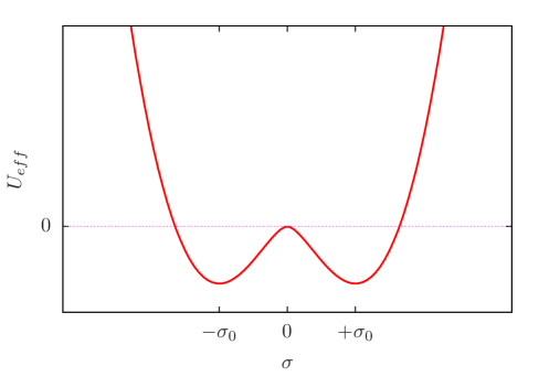
Figure 11: The shape of the function $U_{\mathrm{eff}}$ with respect to $\sigma$. We have defined $\sigma_{0}=\mu e^{-\pi/g(\mu)}$.

One notes that the solution $\sigma=0$ is a local maximum, while the solutions $\sigma=\pm\mu e^{-\pi/g(\mu)}$ represent degenerate absolute minima. Because of the symmetry of $U_{\mathrm{eff}}$ under the change of sign of $\sigma$, any of these can be equivalently chosen. We shall choose for definiteness the solution with a plus sign and shall designate it by $\sigma_{0}$:

$$\sigma_{0}=\mu e^{{\displaystyle-\pi/g(\mu)}}.$$ (59)

In order to study the physical properties of the system around the new ground state, we must shift the field $\sigma$ in the effective potential and in the Lagrangian density by $\sigma_{0}$:

$$\sigma=\sigma^{\prime}+\sigma_{0}.$$ (60)

In terms of the new field $\sigma^{\prime}$, the effective potential becomes

$$U_{\mathrm{eff}}=\frac{N\sigma_{0}^{2}}{4\pi}\ \big{(}1+\frac{\sigma^{\prime}}{\sigma_{0}}\big{)}^{2}\ \Big{[}\ -1+\ln\big{(}1+\frac{\sigma^{\prime}}{\sigma_{0}}\big{)}^{2}\ \Big{]}.$$ (61)

We find that $g(\mu)$ and $\mu$ have completely disappeared from the new expression of $U_{\mathrm{eff}}$ in favor of the single parameter $\sigma_{0}$, which has, by the definition of $\sigma$ [Eq. (44)], a dimension of mass and thus fixes the mass scale of the theory. No free adjustable parameter has remained.

The Lagrangian density becomes:

$$\mathcal{L^{\prime}}=\overline{\psi}^{a}i\gamma^{\mu}\partial_{\mu}\psi^{a}-\frac{N}{2g_{0}}(\sigma^{\prime}+\sigma_{0})^{2}-\sigma_{0}\overline{\psi}^{a}\psi^{a}-\sigma^{\prime}\overline{\psi}^{a}\psi^{a}.$$ (62)

We note the appearance of a mass term of fermions, with value

$$M_{F}=\sigma_{0}=\mu e^{{\displaystyle-\pi/g(\mu)}}.$$ (63)

The Lagrangian density still contains the bare coupling constant $g_{0}$. This is necessary, since one still has to calculate and renormalize the $\sigma^{\prime}$ propagator. The latter receives contributions from the fermion loops which are divergent and whose divergence should be combined with $g_{0}$ to reproduce a finite quantity.

The theory was invariant at the beginning under the discrete chiral transformations, imposing masslessness of the fermions, but now, after renormalization and the shift to the ground state of the energy, the fermions have acquired a mass. This phenomenon is called dynamical mass generation and is due to the spontaneous breaking of the discrete chiral symmetry.

On the other hand, $M_{F}$ is a physical quantity and should not depend on the particular choices of the arbitrary mass parameter $\mu$. From Eq. (63) one notes that $M_{F}$ has two types of dependence on $\mu$: an explicit one and an implicit one through the coupling constant $g(\mu)$ [Eq. (56)]. One verifies that $M_{F}$ is actually independent of $\mu$:

$$\frac{dM_{F}}{d\mu}=\frac{\partial M_{F}}{\partial\mu}+\frac{1}{\mu}\beta(g)\frac{\partial M_{F}}{\partial g}=0.$$ (64)

$M_{F}$ is said to be renormalization group invariant.

Once $M_{F}$ is fixed, the two other parameters, $g$ and $\mu$ should disappear from the finite quantities of the theory. Any choice of $\mu$ is compensated by a corresponding choice of $g$, to produce $M_{F}$. This property was explicitly verified on the expression of $U_{\mathrm{eff}}$ [Eq. (61)].

At the beginning, the theory had a dimensionless parameter $g$ and massless fermions. Now it has instead a dimensionful parameter, $M_{F}$, mass of the fermions, which is fixed by the physical conditions and sets the mass scale of the theory. There is no longer a free parameter in the theory. This phenomenon is called mass transmutation.

In summary, the Gross-Neveu model displays many interesting features of quantum field theory and illustrates, in two dimensions, several phenomena – asymptotic freedom, dynamical mass generation, mass transmutation – expected also to occur in four-dimensional theories.

4 QCD

Quantum Chromodynamics (QCD), the theory of the strong interaction, is a gauge theory with the non-Abelian local symmetry group of color $SU(N)_{c}$, with $N=3$. We consider henceforth the general case where the paramater $N$ is arbitrary. As “matter” fields, the theory contains quark and antiquark fields, belonging to the defining fundamental representation of the group and to its conjugate, respectively; their number is $N$. Since this is a gauge theory, there are also gauge fields, the gluons, belonging to the adjoint representation of the group; their number is $(N^{2}-1)$.

There are six “generations” of QCD, distinguished from each other by specific properties of the quarks (charge and mass), called also “flavors”. Schematically, there are three “light” quarks, $u$, $d$, $s$ and three “heavy” quarks, $c$, $b$, $t$. The free masses of the quarks $u$ and $d$ are of the order of a few MeV, while the mass of the quark $s$ is of the order of 100 MeV. The masses of the heavy quarks $c$, $b$, $t$ are approximately 1.3 GeV, 4.2 GeV and 173 GeV, respectively [15]. The gluon, which is the gauge particle, is massless.

The proton, the stable matter particle, is a bound state made mainly of the three quarks $u$, $u$, $d$. Its mass is of the order of 1 GeV. This shows that the mass of the proton is not made of the masses of its quark components, which are nearly massless. Rather, one should expect that it is produced by a dynamical mass generation mechanism, similar to what happened in the Gross-Neveu model. A similar conclusion also holds for the other low-lying hadrons (neutron, $\rho$ meson, etc.). On the other hand, the coupling constant of the QCD Lagrangian is dimensionless. This means that the mass generation phenomenon would be realized by the mechanism of mass transmutation, which also was observed in the Gross-Neveu model.

Since the light quark masses do not seem to play a fundamental role, one can consider the QCD Lagrangian in the ideal situation where the three light quarks are massless. In this case, the QCD theory also satisfies a global flavor space invariance under the group of continuous chiral transformations $SU(3)_{R}\times SU(3)_{L}$ ($R$ for right, $L$ for left). It is expected that this symmetry is realized with the Goldstone mode (no nearly degenerate parity doublets are observed in nature); the corresponding Goldstone bosons are the lowest lying $\pi$, $K$ and $\eta$ mesons. In the limit of vanishing quark masses, the masses of the latter particles would also vanish. For small values of the quark masses, the Goldstone bosons also acquire a small mass. This explains why these mesons have masses squared much smaller than the other hadron masses squared.

QCD theory has been widely investigated in ordinary perturbation theory and has been shown to be asymptotically free [16, 17]; a relation similar to Eq. (55) has been obtained. This implies that at high energies or at short distances, the QCD interaction becomes weak and ordinary perturbation theory can be applied there. This property has been experimentally verified by many high-energy experiments. The other implication of asymptotic freedom is that at low energies or at large distances the interaction becomes strong enough to forbid perturbative treatments. From asymptotic freedom one also deduces the existence of a renormalization group invariant mass, called $\Lambda_{\mathrm{QCD}}$, which realizes mass transmutation in the theory (cf. Eqs. (59), (63), (64)). Contrary to the Gross-Neveu model, however, the resolution of the nonperturbative domain of QCD has not been achieved up to now with analytic calculations. One of the main reasons of this failure is probably related to the fact that quarks and gluons are confined. These particles have not been observed as free asymptotic states like the other known particles. Their presence or existence have been detected mainly in an indirect way. Quarks and gluons are bound by the QCD force to form bound states called hadrons (proton, neutron, $\pi$ and $\rho$ mesons, etc.) It is at this level that QCD differs from the previous models that were considered or mentioned (Gross-Neveu, Nambu–Jona-Lasinio). Numerical resolution of the strong coupling regime of QCD is successfully realized with Lattice calculations.

The application of the $1/N$ expansion method to QCD leads to some simplifications and well verified qualitative predictions, but fails to solve the theory as a whole. The reason of this last negative result is due to the large number of gluon fields ($\sim N^{2}$) as compared to that of the quarks ($N$). While quark loop contributions become negiligible and do not enter in leading expressions in the large-$N$ limit, gluon loop diagrams, and more precisely the class of “planar diagrams”, become dominant at large $N$ and an infinite number of them (one-particle irreducible) survive [3, 5, 6, 7, 8]. Their summation in compact form is not an easy task. Examples of planar and non-planar diagrams are presented in Figs. 12 and 13, respectively.

Figure 12: Examples of planar diagrams. Curly lines represent gluons and oriented full lines quarks or antiquarks. When a planar diagram is drawn on a plane, a gluon line does not intersect any other gluon line, except at vertices. The latter are represented on the figures by dots.

Figure 13: Examples of non-planer or crossed diagrams. The intersection points of the gluon lines are not vertices.

One therefore is satisfied at the present time with the qualitative predictions and relative simplifications the $1/N$ expansion method provides. The method, when applied to two-dimensional QCD, has been, however, successful enough to solve the main aspects of the theory in an explicit way [4, 18].

5 Conclusion

The $1/N$ expansion method allows us to solve, at leading order of the expansion, theories and models nonperturbatively, probing directly dynamical phenomena, which would not be reached in ordinary perturbation theory based on expansions with respect to the coupling constant.

The method is also applicable to QCD, but because of the presence of the gluon fields, which belong to the adjoint representation of the gauge symmetry group, its effects are less spectacular. Nevertheless, many simplifications occur and several qualitative features can be drawn about the properties of the theory.

Acknowledgements

I thank the Organizing Committee and its members for their invitation and kind hospitality and for the stimulating atmosphere created at the Summer School. This work was partially supported by the EU I3HP Project ”Study of Strongly Interacting Matter” (acronym HadronPhysics3, Grant Agreement No. 283286).

References

- [1] H. E. Stanley, Spherical model as the limit of infinite spin dimensionality, Phys. Rev. 176 (1968) 718.
- [2] K. G. Wilson, Quantum field theory models in less than four-dimensions, Phys. Rev. D 7 (1973) 2911.
- [3] G. ’t Hooft, A planar diagram theory for strong interactions, Nucl. Phys. B 72 (1974) 461.
- [4] G. ’t Hooft, A two-dimensional model for mesons, Nucl. Phys. B 75 (1974) 461.
- [5] E. Witten, Baryons in the expansion, Nucl. Phys. B 160 (1979) 57.
- [6] E. Witten, The expansion in atomic and particle physics, 1979, Lectures at the Cargese Summer School “Recent developments in gauge theories”, edited by G. ’t Hooft et al. (Plenum, N.Y., 1980), p. 403.
- [7] S. R. Coleman, , 1979, Lectures at the Erice International School of Subnuclear Physics (Plenum, N.Y., 1980), p. 805. Also in “Aspects of symmetry” (Cambridge University Press, 1985), p. 351.
- [8] Yu. Makeenko, Large- gauge theories, 1999, Lectures at the NATO-ASI on “Quantum Geometry”, Akureyri, Iceland, NATO Sci. Ser. C 556 (2000) 285 [arXiv: hep-th/0001047].
- [9] S. R. Coleman, R. Jackiw, and H. D. Politzer, Spontaneous symmetry breaking in the model for large , Phys. Rev. D 10 (1974) 2491.
- [10] E. S. Abers and B. W. Lee, Gauge theories, Phys. Rep. 9 (1973) 1.
- [11] S. R. Coleman and E. J. Weinberg, Radiative corrections as the origin of spontaneous symmetry breaking, Phys. Rev. D 7 (1973) 1888.
- [12] R. Jackiw, Functional evaluation of the effective potential, Phys. Rev. D 9 (1974) 1686.
- [13] Y. Nambu and G. Jona-Lasinio, Dynamical model of elementary particles based on an analogy with superconductivity. 1, Phys. Rev. 122 (1961) 345.
- [14] D. J. Gross and A. Neveu, Dynamical symmetry breaking in asymptotically free field theories, Phys. Rev. D 10 (1974) 3235.
- [15] K. A. Olive et al. (Particle Data Group), Review of particle physics, Chin. Phys. C 38 (2014) 090001.
- [16] D. J. Gross and F. Wilczek, Ultraviolet behavior of non-Abelian gauge theories, Phys. Rev. Lett. 30 (1973) 1343.
- [17] H. D. Politzer, Reliable perturbative results for strong interactions?, Phys. Rev. Lett. 30 (1973) 1346.
- [18] C. G. Callan, Jr., N. Coote, and D. J. Gross, Two-dimensional Yang-Mills theory: A model of quark confinement, Phys. Rev. D 13 (1976) 1649.