Abstract

We present new method for the numerical reconstruction of the variable refractive index of multi-layered circular weakly guiding dielectric waveguides using the measurements of the propagation constants of their eigenwaves. Our numerical examples show stable reconstruction of the dielectric permittivity function $\varepsilon$ for random noise level using these measurements.

1 Introduction

The development of analytical methods for the study of mathematical models, the development and the justification of efficient numerical methods for the solution of spectral problems of the theory of dielectric waveguides attract the much attention (see, for example, [3, 6, 12]). Dielectric waveguides form the basic components of the microdevices used in the field of integrated optics, photonics, and laser technology. The development of analytical methods for the study of mathematical models of optical microdevices, the development of numerical methods for accurate and stable computations of their characteristics are essential for designing and optimizing of such devices.

The problem of reconstruction of the refractive index of an inhomogeneous dielectric waveguide from the measurements of the propagation constants of its eigenwaves is very urgent. Universal numerical methods of reconstruction of refractive index of dielectric objects are designed for coefficient inverse diffraction problems and ignore the waveguide properties of the devices (see, for example, [4]). The methods for the determination of the optical characteristics of dielectric waveguides are proposed for waveguides of some special forms (see, for example, [16, 18]). For instance, the waveguide spectroscopy is widely used for planar (one-dimensional) multi-layered waveguides [11]. For such waveguides the characteristic equation (a transcendental equation which connects the refractive indices of the waveguide’s layers with the propagation constants of its eigenwaves) is well known. The method consists in minimization of a functional, depending on the refractive indices of the layers. The value of the functional is equal to the distance between the vector of calculated (as the roots of the characteristic equation) propagation constants and the vector of experimentally measured propagation constants. Considerable efforts have been directed towards the development of effective methods of minimization of this functional [13, 14].

This method was extended in our previous works to the two-dimensional problem for the waveguide with the piecewise-constant refractive index and an arbitrary cross-sectional boundary [8, 9]. The role of the “characteristic equation" is played by the system of two boundary weakly singular integral equations whose kernels depend on the propagation constants and refractive indices of the vaweguide and the environment. We presented new numerical methods for the solution of the inverse spectral problem to determine the dielectric constants of core and cladding in optical fibers. These methods use measurements of propagation constants. Our algorithms are based on approximate solution of a nonlinear nonselfadjoint eigenvalue problem for a system of weakly singular integral equations. We studied the inverse problem and proved that it is well posed. Our numerical results indicated good accuracy of new algorithms. Clearly, the generalization of this method for an inhomogeneous waveguide is an urgent task. Theoretical justification of this method is a very interesting problem.

In the presented paper we construct a Tikhonov functional and propose a method for the numerical reconstruction of the variable refractive index of multi-layered circular weakly guiding dielectric waveguides from the measurements of the propagation constants of their eigenwaves. We theoretically investigate the Tikhonov functional and demonstrate the practical effectiveness of the proposed method. The success in the Tikhonov regularization method largely depends on a good initial approximation to the solution. The matematical analysis of the forward problem has allowed us to find a good first approximation to the refractive index of the waveguide [7, 19]. This is confirmed by the numerical experiments of solving the similar inverse problems [8, 9]. Using this initial approximation, in this paper we compute solutions of the investigated problem and demonstrate that the algorithm is accurate and stable.

2 Main equations

Let us consider a multi-layered circular optical fiber shown at Figure  1 as a regular cylindrical dielectric waveguide in a free space. The axis of the cylinder is parallel to the $x_{3}$-axis. Suppose that the circles separating the layers of the waveguide have the radiuses $r_{l}$, $l=1,\,2,\,\ldots,\,n$. Let the permittivity be prescribed as a positive piecewise constant function $\varepsilon$ which is equal to a constant $\varepsilon_{e}$ for $r=\sqrt{x_{1}^{2}+x_{2}^{2}}>r_{n}$ and to constants $\varepsilon_{l}$, where $l=1,\,2,\,\ldots,\,n$, in corresponding layers. Let us denote $\varepsilon_{+}=\max\limits_{l=1,\,2,\,\ldots,\,n}\varepsilon_{l}$, and suppose that

$$\min\limits_{l=1,\ldots,n}\varepsilon_{l}>\varepsilon_{e}\geq 1.$$ (1)

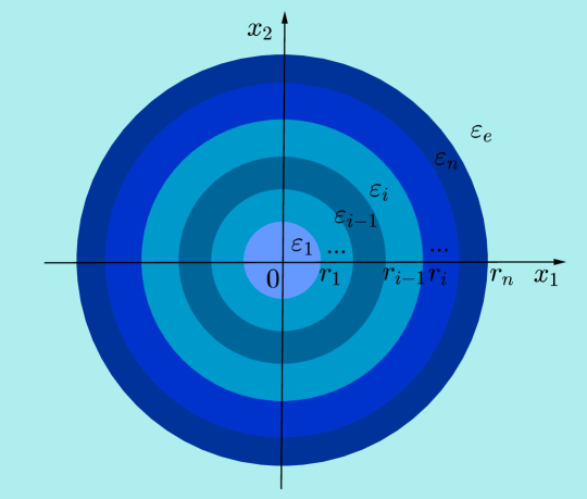
Figure 1: Geometry of a multi-layered circular optical fiber

Eigenvalue problems of optical waveguide theory [15] are formulated on the base of the set of homogeneous Maxwell equations

$$\begin{array}[]{c}\displaystyle{\textrm{rot}\cal E=}-\mu_{0}\frac{{\partial{\cal H}}}{{\partial t}},\quad{\textrm{rot}\cal H=}\varepsilon_{0}\varepsilon\frac{{\partial{\cal E}}}{{\partial t}}.\end{array}$$ (2)

Here, $\cal E$ and $\cal H$ are electric and magnetic field vectors; $\varepsilon_{0}$ and $\mu_{0}$ are the free-space dielectric and magnetic constants. Nontrivial solutions of set (2) which have the form

$$\begin{array}[]{c}\displaystyle\left[{\begin{array}[]{*{20}c}{\cal E}\\ {\cal H}\\ \end{array}}\right](x,x_{3},t)={\mathop{\rm Re}\nolimits}\left({\left[{\begin{array}[]{*{20}c}{\rm E}\\ {\rm H}\\ \end{array}}\right](x)e^{i(\beta x_{3}-\omega t)}}\right)\end{array}$$ (3)

are called the eigenwaves of the waveguide. Here, positive $\omega$ is the radian frequency, $\beta$ is the propagation constant, $\rm E$ and $\rm H$ are complex amplitudes of $\cal E$ and $\cal H$, $x=(x_{1},x_{2})$.

In forward eigenvalue problems the permittivity is known and it is necessary to calculate longitudinal wavenumbers $k=\omega\sqrt{\varepsilon_{0}\mu_{0}}$ and propagation constants $\beta$ such that there exist eigenmodes. The eigenmodes have to satisfy transparency conditions at the boundaries and satisfy an condition at infinity. In inverse problems considering in this work it is necessary to reconstruct the unknown permittivity $\varepsilon$ by some information on natural eigenwaves which exist for some eigenvalues $k$ and $\beta$.

The domain $\Omega_{e}=\{x\in\mathbb{R}^{2}:r>r_{n}\}$ is unbounded. Therefore, it is necessary to formulate a condition at infinity for complex amplitudes $\mathrm{E}$ and $\mathrm{H}$ of eigenmodes. Let us confine ourselves to the investigation of the surface modes only. The propagation constants $\beta$ of surface modes are real and belong to the interval $G=(k\varepsilon_{e},k\varepsilon_{+})$. The amplitudes of surface modes satisfy to the following condition:

$$\left[{\begin{array}[]{*{20}c}{\rm E}\\ {\rm H}\\ \end{array}}\right]=e^{{-\sigma r}}O\left({\frac{1}{\sqrt{r}}}\right),\quad r\rightarrow\infty.$$ (4)

Here, $\sigma=\sqrt{\beta^{2}-k^{2}\varepsilon_{e}}>0$ is the transverse wavenumber in the cladding.

Denote by $\chi_{l}=\sqrt{k^{2}\varepsilon_{l}-\beta^{2}}$ the transverse wavenumbers in the waveguide’s layers. Under the weakly guidance approximation [15] the original problem is reduced to the calculation of numbers $k$ and $\beta$ such that there exist nontrivial solutions $u=\rm H_{1}=H_{2}$ of Helmholtz equations

$$\Delta u+\chi_{l}^{2}u=0,\quad x\in\Omega_{l},\quad l=1,\,2,\,\ldots,\,n,$$ (5)

$$\Delta u-\sigma^{2}u=0,\quad x\in\Omega_{e},$$ (6)

which satisfy the transparency conditions

$$u^{+}=u^{-},\quad\frac{\partial u^{+}}{\partial r}=\frac{\partial u^{-}}{\partial r},\quad x\in\gamma_{l},\quad l=1,\,2,\,\ldots,\,n.$$ (7)

Here $\Omega_{1}=\{x\in\mathbb{R}^{2}:r<r_{1}\}$, $\Omega_{l}=\{x\in\mathbb{R}^{2}:r_{l-1}<r<r_{l}\}$, $\gamma_{l}=\{x\in\mathbb{R}^{2}:r=r_{l}\}$, $l=1,\,2,\,\ldots,\,n$; $u^{-}$ (respectively, $u^{+}$) is the limit value of a function $u$ from the interior (respectively, the exterior) of $\gamma_{l}$.

Let us calculate nontrivial solutions $u$ of problem (5)–(7) in the space of continuous and continuously differentiable in $\overline{\Omega}_{e}$ and $\overline{\Omega}_{l}$, $l=1,\,2,\,\ldots,\,n$, and twice continuously differentiable in $\Omega_{e}$ and $\Omega_{l}$, $l=1,\,2,\,\ldots,\,n$, functions, satisfying condition

$$u=e^{{-\sigma r}}O\left({\frac{1}{\sqrt{r}}}\right),\quad r\rightarrow\infty.$$ (8)

Denote by $U$ described functional space. We solve problem (5)–(7) by the method of separation of variables using polar coordinates $(r,\varphi)$ and look for the function $u\in U\setminus\{0\}$ in the form

$$u(r,\varphi)=R(r)\Phi(\varphi).$$ (9)

Then

$$\Phi(\varphi)=\left\{\begin{array}[]{c}\cos m\varphi\\ \sin m\varphi\\ \end{array}\right.,\quad m=0,\,1,\,2,\,\ldots,$$

$$R(r)=\left\{\begin{array}[]{c}aJ_{m}(\chi_{1}r),\quad r<r_{1}\\ b_{l}J_{m}(\chi_{l}r)+c_{l}H_{m}^{(1)}(\chi_{l}r),\quad r_{l-1}<r<r_{l},\quad l=2,\,\ldots,\,n\\ dK_{m}(\sigma r),\quad r>r_{n}.\\ \end{array}\right.,$$

here $J_{m}(z)$ is the Bessel function, $H_{m}^{(1)}(z)$ is the Hankel function of the first kind, $K_{m}(z)$ is the Macdonald function. Unknown coefficients $a$, $b_{l}$, $c_{l}$, and $d$ satisfy the following homogeneous system of linear algebraic equations:

$$\left(\begin{array}[]{cccc}A_{11}(k,\beta,\varepsilon_{1},\varepsilon_{2})&0&\ldots&0\\ 0&A_{22}(k,\beta,\varepsilon_{2},\varepsilon_{3})&\ldots&0\\ \ldots&\ldots&\ldots&\ldots\\ 0&0&\ldots&A_{nn}(k,\beta,\varepsilon_{n},\varepsilon_{e})\\ \end{array}\right)\left(\begin{array}[]{c}X_{1}\\ X_{2}\\ \ldots\\ X_{n}\\ \end{array}\right)=0.$$ (10)

Here

$$A_{11}(k,\beta,\varepsilon_{1},\varepsilon_{2})=\left(\begin{array}[]{ccc}J_{m}(\chi_{1}r_{1})&-J_{m}(\chi_{2}r_{1})&-H_{m}^{(1)}(\chi_{2}r_{1})\\ \chi_{1}J^{\prime}_{m}(\chi_{1}r_{1})&-\chi_{2}J^{\prime}_{m}(\chi_{2}r_{1})&-\chi_{2}H_{m}^{(1)^{\prime}}(\chi_{2}r_{1})\\ \end{array}\right),$$

$$A_{nn}(k,\beta,\varepsilon_{n},\varepsilon_{e})=\left(\begin{array}[]{ccc}J_{m}(\chi_{n}r_{n})&H_{m}^{(1)}(\chi_{n}r_{n})&-K_{m}(\sigma r_{n})\\ \chi_{n}J^{\prime}_{m}(\chi_{n}r_{n})&\chi_{n}H_{m}^{(1)^{\prime}}(\chi_{n}r_{n})&-\sigma K^{\prime}_{m}(\sigma r_{n})\\ \end{array}\right),$$

$$A_{ll}(k,\beta,\varepsilon_{l},\varepsilon_{l+1})=$$

$$=\left(\begin{array}[]{cccc}J_{m}(\chi_{l}r_{l})&H_{m}^{(1)}(\chi_{l}r_{l})&-J_{m}(\chi_{l+1}r_{l})&-H_{m}^{(1)}(\chi_{l+1}r_{l})\\ \chi_{l}J^{\prime}_{m}(\chi_{l}r_{l})&\chi_{l}H_{m}^{(1)^{\prime}}(\chi_{l}r_{l})&-\chi_{l+1}J^{\prime}_{m}(\chi_{l+1}r_{l})&-\chi_{l+1}H_{m}^{(1)^{\prime}}(\chi_{l+1}r_{l})\\ \end{array}\right),$$

$$X_{1}=\left(\begin{array}[]{c}a\\ b_{2}\\ c_{2}\\ \end{array}\right),\ X_{n}=\left(\begin{array}[]{c}b_{n}\\ c_{n}\\ d\\ \end{array}\right),\ X_{l}=\left(\begin{array}[]{c}b_{l}\\ c_{l}\\ b_{l+1}\\ c_{l+1}\\ \end{array}\right),$$

where $l=2,\,3,\,\ldots,\,n-1$. System (10) has a nontrivial solution if and only if the determinant of its matrix is equal to zero:

$$\det(A(k,\beta,\varepsilon))=0.$$ (11)

The last condition in the theory of optical waveguides is called the characteristic equation.

3 Ill-posed problems

In this section on the base of characteristic equation (11) we formulate problems of reconstruction of the unknown permittivity $\varepsilon$ by some information on the fundamental eigenwaves which exist for some $k$ and $\beta$. In the case of the fundamental eigenwave the permittivity $\varepsilon$ are connected with each value of the propagation constant $\beta$ and each value of the longitudinal wavenumber $k$ by characteristic equation (11) with $m=0$:

$$\det(A(k,\beta,\varepsilon))=\left|\begin{array}[]{cccc}A_{11}(k,\beta,\varepsilon_{1},\varepsilon_{2})&0&\ldots&0\\ 0&A_{22}(k,\beta,\varepsilon_{2},\varepsilon_{3})&\ldots&0\\ \ldots&\ldots&\ldots&\ldots\\ 0&0&\ldots&A_{nn}(k,\beta,\varepsilon_{n},\varepsilon_{e})\\ \end{array}\right|=0.$$ (12)

Here

$$A_{11}(k,\beta,\varepsilon_{1},\varepsilon_{2})=\left(\begin{array}[]{ccc}J_{0}(\chi_{1}r_{1})&-J_{0}(\chi_{2}r_{1})&-H_{0}^{(1)}(\chi_{2}r_{1})\\ \chi_{1}J^{\prime}_{0}(\chi_{1}r_{1})&-\chi_{2}J^{\prime}_{0}(\chi_{2}r_{1})&-\chi_{2}H_{0}^{(1)^{\prime}}(\chi_{2}r_{1})\\ \end{array}\right),$$

$$A_{nn}(k,\beta,\varepsilon_{n},\varepsilon_{e})=\left(\begin{array}[]{ccc}J_{0}(\chi_{n}r_{n})&H_{0}^{(1)}(\chi_{n}r_{n})&-K_{0}(\sigma r_{n})\\ \chi_{n}J^{\prime}_{0}(\chi_{n}r_{n})&\chi_{n}H_{0}^{(1)^{\prime}}(\chi_{n}r_{n})&-\sigma K^{\prime}_{0}(\sigma r_{n})\\ \end{array}\right),$$

$$A_{ll}(k,\beta,\varepsilon_{l},\varepsilon_{l+1})=$$

$$=\left(\begin{array}[]{cccc}J_{0}(\chi_{l}r_{l})&H_{0}^{(1)}(\chi_{l}r_{l})&-J_{0}(\chi_{l+1}r_{l})&-H_{0}^{(1)}(\chi_{l+1}r_{l})\\ \chi_{l}J^{\prime}_{0}(\chi_{l}r_{l})&\chi_{l}H_{0}^{(1)^{\prime}}(\chi_{l}r_{l})&-\chi_{l+1}J^{\prime}_{0}(\chi_{l+1}r_{l})&-\chi_{l+1}H_{0}^{(1)^{\prime}}(\chi_{l+1}r_{l})\\ \end{array}\right),$$

where $l=2,\,3,\,\ldots,\,n-1$.

We suppose that the permittivities $\varepsilon_{1}$, $\varepsilon_{2}$, … $\varepsilon_{n}$, $\varepsilon_{e}$ are real and satisfy conditions (1). Denote by $\varepsilon=(\varepsilon_{1},\varepsilon_{2},\ldots,\varepsilon_{n},\varepsilon_{e})\in\mathbb{R}^{n+1}$ the vector of the permittivities of the waveguide. Then we can write condition (1) in the matrix form:

$$C\varepsilon\leq q,$$ (13)

$$C=\left(\begin{array}[]{ccccc}\phantom{-}0&0&\ldots&\phantom{-}0&-1\\ -1&0&\ldots&\phantom{-}0&\phantom{-}1\\ \phantom{-}\ldots&\ldots&\phantom{-}\ldots&\ldots&\phantom{-}\ldots\\ \phantom{-}0&0&\ldots&-1&\phantom{-}1\\ \end{array}\right),\quad q=\left(\begin{array}[]{c}-1\\ -\mu\\ -\mu\\ -\mu\\ \end{array}\right),$$

where $\mu$ is a small positive number.

Suppose that we know $m\geq n+1$ pairs of values of the longitudinal wavenumber and the propagation constant of the fundamental eigenwave of the waveguide: $(k_{i},\beta_{i})$, $i=1,\,2,\,\ldots,\,m$. Let us introduce $m$ functions $f_{i}(\varepsilon)$ of the variable $\varepsilon$ by the following way:

$$f_{i}(\varepsilon)=1/\textrm{cond}(A(k_{i},\beta_{i},\varepsilon)),\quad i=1,\,2,\,\ldots,\,m.$$

Here $A$ is the matrix defined in (12). By cond we denote the condition number of $A$. Clearly, all $f_{i}$ are non-negative and if $\varepsilon$ satisfies characteristic equation (12), then $f_{i}(\varepsilon)=0$, $i=1,\,2,\,\ldots,\,m$. Let us introduce the nonlinear operator $F:\mathbb{R}^{n+1}\to\mathbb{R}^{m}$ by the formula:

$$F(\varepsilon)=(f_{1}(\varepsilon),f_{2}(\varepsilon),\ldots,f_{m}(\varepsilon)).$$

It seems natural to find the vector $\varepsilon$ of the permittivities as a solution of the problem

$$F(\varepsilon)=0,\quad C\varepsilon\leq q,$$ (14)

it also seems useful to study along with (14) the minimization problem

$$\min\limits_{C\varepsilon\leq q}\frac{1}{2}||F(\varepsilon)||^{2}_{\mathbb{R}^{m}},$$ (15)

but this way is not correct. Problems (14) and (15) are not equivalent; each solution of (14) is evidently a global minimizer of problem (15) while a solution of (15) do not necessarily satisfy (14). Moreover, problems (14) and (15) are ill-posed (see, for example [2]). The ill-posedness of these problems means that analyzing problems close in some sense to (14) and (15), we can not guarantee that solutions to these perturbed problems are close to corresponding solutions of the original ones.

4 The Tikhonov functional

In real-life applications for each fixed longitudinal wavenumber the propagation constant of the fundamental eigenwave of the waveguide is measured by physical experiments. Denote by $({k}_{i},\widetilde{\beta}_{i})$, $i=1,\,2,\,\ldots,\,m$, these values. Denote by $\widetilde{F}:\mathbb{R}^{n+1}\to\mathbb{R}^{m}$ the perturbed operator, where

$$\widetilde{F}(\varepsilon)=(\widetilde{f}_{1}(\varepsilon),\widetilde{f}_{2}(\varepsilon),\ldots,\widetilde{f}_{m}(\varepsilon)),$$

$$\widetilde{f}_{i}(\varepsilon)=1/\textrm{cond}(A({k}_{i},\widetilde{\beta}_{i},\varepsilon)),\quad i=1,\,2,\,\ldots,\,m.$$

Therefore instead of original problem (14) we have perturbed problem

$$\widetilde{F}(\varepsilon)=0,\quad C\varepsilon\leq q.$$ (16)

We suppose that the perturbation is small, namely,

$$||\widetilde{F}(\varepsilon_{*})||_{\mathbb{R}^{m}}\leq\delta.$$

Here the small parameter $\delta\in(0,1)$ characterizes the level of the error in data, $\varepsilon_{*}$ is the exact solution of non-perturbed problem (14).

As we have seen, problem (14) is a classical ill-posed problem [20]. Thus, we assume that there exists the exact solution $\varepsilon_{*}$ to our problem (14) but we never will get this solution in computations. Because of that we call by the regularized solution $\varepsilon_{\alpha}$ some approximation of the unknown exact solution $\varepsilon_{*}$ which is satisfied to the requirements of closeness to the exact solution $\varepsilon_{*}$ and stability with respect to the small errors $\delta$.

We use Tikhonov regularization algorithm (see [20]) which is based on the minimization of the Tikhonov functional. Thus, to find regularized solution $\varepsilon_{\alpha}$ of problem (16), we minimize the Tikhonov regularization functional

$$M_{\alpha}(\varepsilon)=\frac{1}{2}\left\|\widetilde{F}(\varepsilon)\right\|_{\mathbb{R}^{m}}^{2}+\frac{\alpha}{2}\left\|\varepsilon-\varepsilon_{0}\right\|_{\mathbb{R}^{n+1}}^{2},\quad C\varepsilon\leq q,$$ (17)

$$M_{\alpha}:\mathbb{R}^{n+1}\rightarrow\mathbb{R},\quad\varepsilon_{0}\in\mathbb{R}^{n+1},$$

where $\alpha=\alpha\left(\delta\right)>0$ is a small regularization parameter. The choice of the point $\varepsilon_{0}$ and the regularization parameter $\alpha$ depends on the concrete minimization problem. This question will be investigated later by numerical experiments. Usually $\varepsilon_{0}$ is a good first approximation for the exact solution $\varepsilon_{*}.$

It follows from [20] that an algorithm for solution of the equation (16) which is based on the minimization of the Tikhonov functional (17) is the regularization algorithm, and the element $\varepsilon_{\alpha}\in\mathbb{R}^{n+1}$ where the functional (17) reaches its minimum is the regularized solution.

In our theoretical investigations below we need reformulate results of [5, 4] for the case of our IP. In this section below $||\cdot||$ denotes $\mathbb{R}^{n+1}$ norm. Let $H_{1}$ be the finite dimensional linear space. Let $Y$ be the set of admissible parameters for $\varepsilon\in\mathbb{R}^{n+1}$ defined in (13) and let us define by $Y_{1}:=Y\cap H_{1}$ with $G:=\bar{Y}_{1}$. Now the operator $\widetilde{F}:G\to H_{2}$ corresponds to the operator in the Tikhonov functional (17).

We now assume that the operator $\widetilde{F}(\varepsilon)$ defined in (16) is one-to-one and denote by $V_{r}\left(\varepsilon\right)$ neighborhood of the radius $r$ of $\varepsilon$ such that

$$V_{r}\left(\varepsilon\right)=\left\{\varepsilon^{\prime}\in H_{1}:\left\|\varepsilon^{\prime}-\varepsilon\right\|<r,~{}~{}\forall r>0~{}~{}\forall\varepsilon\in H_{1}\right\}.$$ (18)

We also make common assumptions, see for details [1, 21], that the operator $\widetilde{F}$ has the Lipschitz continuous Frechét derivative $\widetilde{F}^{\prime}(\varepsilon)$ for $\varepsilon\in V_{1}(\varepsilon^{\ast}),$ such that there exist constants $N_{1},N_{2}>0$

$$\left\|\widetilde{F}^{\prime}(\varepsilon)\right\|\leq N_{1},\left\|\widetilde{F}^{\prime}(\varepsilon_{1})-\widetilde{F}^{\prime}(\varepsilon_{2})\right\|\leq N_{2}\left\|\varepsilon_{1}-\varepsilon_{2}\right\|,\forall\varepsilon_{1},\varepsilon_{2}\in V_{1}\left(\varepsilon^{\ast}\right).$$ (19)

Similarly with [5] we choose the constant $D=D\left(N_{1},N_{2}\right)=const.>0$ such that

$$|M_{\alpha}^{\prime}(\varepsilon_{1})-M_{\alpha}^{\prime}(\varepsilon_{2})|\leq D\left\|\varepsilon_{1}-\varepsilon_{2}\right\|,\forall\varepsilon_{1},\varepsilon_{2}\in V_{1}(\varepsilon^{*}).$$ (20)

Through the paper as in [5] we assume that

$$\left\|\varepsilon_{0}-\varepsilon^{\ast}\right\| \leq \delta^{\xi},~{}\xi=const.\in\left(0,1\right),$$ (21)

$$\alpha = \delta^{\zeta},\zeta=const.\in(0,\min(\xi,2-2\xi)),$$ (22)

where $\alpha$ is the regularization parameter. Equation (21) means that we assume that all initial guess $\varepsilon_{0}$ in the Tikhonov functional is located in a sufficiently small neighborhood $V_{\delta^{\xi}}(\varepsilon^{*})$ of the exact solution $\varepsilon^{*}$. From Lemmata 2.1 and 3.2 of [5] follows that conditions (22) ensures that $(\varepsilon^{\ast},\varepsilon_{0})$ belong to an appropriate neighborhood of the regularized solution of the Tikhonov functiona.

Below we reformulate Theorem 1.9.1.2 of [4] for the case of our Tikhonov functional. Different proofs of this theorem can be found in [4] and in [5] and are straightly applied to our case.

Theorem 1 Let $\Omega\subset\mathbb{R}^{3}$  be a convex bounded domain with the boundary $\partial\Omega\in C^{3}.$ Assume that there exists the exact solution $\varepsilon^{*}\in G$ of the equation $\widetilde{F}(\varepsilon^{*})=0$  for the case of the exact data $(k_{i}^{\ast},\beta_{i}^{\ast})$. Let regularization parameter $\alpha$ in (17) is such that

$$\alpha=\alpha(\delta)=\delta^{2\nu},~{}~{}\nu=const.\in\left(0,\frac{1}{4}\right),~{}\quad\forall\delta\in\left(0,1\right).$$

Let $\varepsilon_{0}$ satisfies conditions (21). Then the Tikhonov functional (17) is strongly convex in the neighborhood $V_{\alpha}\left(\delta\right)(\varepsilon^{*})$  with the strong convexity constant $\gamma=\alpha.$ The strong convexity property can be also written as

$$\left\|\varepsilon_{1}-\varepsilon_{2}\right\|^{2}\leq\frac{2}{\delta^{2\nu}}\left(M_{\alpha}^{\prime}(\varepsilon_{1})-M_{\alpha}^{\prime}(\varepsilon_{2}),\varepsilon_{1}-\varepsilon_{2}\right),\text{ }\forall\varepsilon_{1},\varepsilon_{2}\in H_{1},$$ (23)

where $(\cdot,\cdot)$ is a scalar product. Next, there exists the unique regularized solution $\varepsilon_{\alpha}$ of the functional (17) and this solution $\varepsilon_{\alpha}\in V_{\delta^{3\nu}/3}(\varepsilon^{*}).$ The gradient method of the minimization of the functional (17) which starts at $\varepsilon_{0}$ converges to the regularized solution of this functional. Furthermore,

$$\left\|\varepsilon_{\alpha}-\varepsilon^{*}\right\|\leq\theta\left\|\varepsilon_{0}-\varepsilon^{*}\right\|,~{}~{}\theta\in(0,1).$$ (24)

The property(24) means that the regularized solution of the Tikhonov functional (17) provides a better accuracy than the initial guess $\varepsilon_{0}$ if it satisfies condition (21).

5 Numerical experiments

We minimized the Tikhonov functional (17) using the GlobalSearch Algorithm of the GlobalSearch object in MATLAB in the case of the one-layered waveguide. The exact values of parameters are chosen as follows: $\varepsilon_{i}=\varepsilon_{1}=2.383936$ (quartz) and $\varepsilon_{e}=2.21235876$ (optical glass). The exact solutions $(k_{i}^{2},\beta_{i}^{2})$ of the forward spectral problem for this waveguide are well known (see, for example, [19]). We constructed the Tikhonov functional using five pairs of eigenvalues corresponding to the fundamental eigenwave, see Table 1.

Table 1. Five pairs of eigenvalues corresponding to the fundamental eigenwave which are used in numerical tests.

$i$	$k_{i}^{2}$	$\beta_{i}^{2}$
1	02.4	05.30978783787819
2	04.8	10.63618822212100
3	07.2	16.02129849868130
4	09.6	21.46863534179760
5	12.0	26.96464966481510

It follows from the results of [19] that for the wide range of frequencies the following formula gives a very good approximation from above to the permittivity $\varepsilon_{e}$ of the cladding of the waveguide:

$$\varepsilon_{e}\approx{\beta_{1}^{2}}/{k_{1}^{2}}.$$

Using this formula and condition (13), we took the first approximation to the vector of permittivities $\varepsilon=(\varepsilon_{i},\,\varepsilon_{e})$ as

$$\varepsilon_{0}=(\varepsilon_{0,i},\varepsilon_{0,e})=({\beta_{1}^{2}}/{k_{1}^{2}},\,{\beta_{1}^{2}}/{k_{1}^{2}})=(2.21241159911591,\,2.21241159911591).$$

In our computations by analogy with [8] we introduced a randomly distributed noise in the propagation constants as

$$\widetilde{\beta_{i}}=\beta_{i}(1+p\alpha),\quad i=1,\,2,\,\ldots\,5,$$

where $\beta_{i}$ are the exact measured propagation constants, $\alpha\in(-1,1)$ are randomly distributed numbers, and $p$ is the noise level. In our computations we used $p=0.05$ and thus, the noise level was $5\%$. In the numerical experiments we accounted this noise in perturbed operator (16) and also in the perturbed initial approximations

$$\widetilde{\varepsilon}_{0}=(\widetilde{\varepsilon}_{0,i},\widetilde{\varepsilon}_{0,e})=({\widetilde{\beta}_{1}^{2}}/{k_{1}^{2}},\,{\widetilde{\beta}_{1}^{2}}/{k_{1}^{2}})$$

that we used in (17) instead of $\varepsilon_{0}$. The regularization parameter was $\alpha=0.01$.

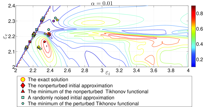
Figure 2: The results of numerical minimization of the nonperturbed and perturbed (by the randomly noised propagation constants $\widetilde{\beta_{i}}$ with the $5\%$ noise level) Tikhonov functional. The background is the pattern of the nonperturbed functional.

Some numerical results of reconstruction of the vector $\varepsilon$ of the permittivies are presented at Figure 2. The exact value $\varepsilon$ is marked at Figure  2 by the big yellow circle. The approximated value

$$\varepsilon_{\alpha}=(2.38393603911088,\,2.21235872913944)$$

of $\varepsilon$ for the noise-free data is marked by the red triangle. The background of this figure is the pattern of the nonperturbed Tikhonov functional. Approximated values $\widetilde{\varepsilon}_{\alpha}=(\widetilde{\varepsilon}_{\alpha,i},\widetilde{\varepsilon}_{\alpha,e})$ of $\varepsilon$ for randomly distributed noise $\widetilde{\beta_{i}}$ with the $5\%$ noise level are marked by the colored circles. The nonperturbed initial approximation ${\varepsilon}_{0}$ is marked by the red rhomb, and the perturbed initial approximations $\widetilde{\varepsilon}_{0}$ are marked by the colored squares. The Table 2 presents results of the reconstruction for different initial guesses with random noise level $\sigma=5\%$ in data. Using the Figure 3 and the Table 2 we observe that the approximate solutions were stable even for the randomly noised $\widetilde{\beta_{i}}$. Using the Table 2 we also observe that the computed relative error $e={\|\varepsilon-\widetilde{\varepsilon}_{\alpha}\|_{\mathbb{R}^{2}}}/{\|\varepsilon\|_{\mathbb{R}^{2}}}$ is on the interval $[0,\,0.05]$, and thus, approximated values $\widetilde{\varepsilon}_{\alpha}$ differs from the exact values of $\varepsilon$ not more than $5\%$.

Table 2. Computational results of the reconstructions $\widetilde{\varepsilon}_{\alpha,i},\widetilde{\varepsilon}_{\alpha,e}$ together with computational errors $e$ for different initial guesses $\widetilde{\varepsilon}_{0,i}=\widetilde{\varepsilon}_{0,e}$. Noise in data is $\sigma=5\%$.

$\widetilde{\varepsilon}_{0,i}=\widetilde{\varepsilon}_{0,e}$	$\widetilde{\varepsilon}_{\alpha,i}$	$\widetilde{\varepsilon}_{\alpha,e}$	$e$
2.11768385759666	2.28552927271664	2.11830350061034	0.04186
2.12734296884777	2.26254671102130	2.15032840068311	0.04192
2.13098610290990	2.26628839765012	2.15401089492431	0.04038
2.16434434702641	2.33397022113028	2.16467608183591	0.02124
2.20248954651734	2.37362289984480	2.20251745727489	0.00439
2.21597381604893	2.34013490935047	2.25067212773741	0.01790
2.24374276867624	2.38204127941254	2.26798587326534	0.01712
2.29968977385246	2.43945637236437	2.32453737220619	0.03849
2.30737609305936	2.48261925050832	2.30651724858946	0.04194
2.31946862194614	2.45975978096066	2.34452993693523	0.04686

Analogous results we obtained for the $20\%$ noise level. We present reconstruction results in Figure 3 and in the Table 3. Using the Table 3 we see, that the relative error $e$ is located on the interval $[0,\,0.20]$, and approximated values $\widetilde{\varepsilon}_{\alpha}$ differs from the exact values of $\varepsilon$ not more than $20\%$.

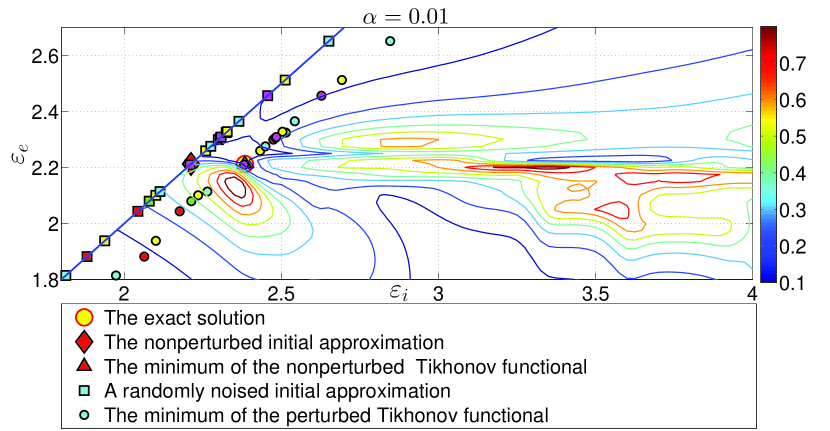
Figure 3: The results of numerical minimization of the nonperturbed and perturbed (by the randomly noised propagation constants $\widetilde{\beta_{i}}$ with the $20\%$ noise level) Tikhonov functional. The background is the pattern of the nonperturbed functional.

Table 3. Computational results of the reconstructions $\widetilde{\varepsilon}_{\alpha,i},\widetilde{\varepsilon}_{\alpha,e}$ together with computational errors $e$ for different initial guesses $\widetilde{\varepsilon}_{0,i}=\widetilde{\varepsilon}_{0,e}$. Noise in data is $\sigma=20\%$.

$\widetilde{\varepsilon}_{0,i}=\widetilde{\varepsilon}_{0,e}$	$\widetilde{\varepsilon}_{\alpha,i}$	$\widetilde{\varepsilon}_{\alpha,e}$	$e$
1.81417751127505	1.97381469634454	1.81480974434505	0.17563
1.88178880974403	2.06363445374894	1.87910974743464	0.14212
1.93807256082554	2.10049008805235	1.93817330919554	0.12126
2.04345147329207	2.17638931794059	2.06553048164261	0.07817
2.07966690316895	2.21358678746843	2.10213721049311	0.06239
2.10053329208657	2.23501858364500	2.12322904231478	0.05337
2.11410009015371	2.26444198310842	2.14720323360852	0.04185
2.20972436445250	2.38114288964767	2.20969348288490	0.00119
2.25920990213314	2.43257430919639	2.25876527535809	0.02067
2.27540878243121	2.44940844145173	2.27482428589175	0.02783
2.29950015590045	2.47444275383217	2.29870392359414	0.03847
2.30564544562698	2.48082751592143	2.30479520038292	0.04118
2.30861157840774	2.48391025002180	2.30773406680037	0.04249
2.32443445081245	2.51439918461942	2.36083107170200	0.06078
2.32757009410069	2.50359310544044	2.32653791258360	0.05086
2.36509793984544	2.54259737446660	2.36370206817162	0.06742
2.45636539769611	2.62761067485400	2.45337536941920	0.10539
2.51223352049175	2.69257246813461	2.51223352049175	0.13232
2.65120325027458	2.84608346134752	2.64927524365834	0.19555

Using Tables 2, 3 and Figures 2, 3 we conclude that the optimization algorithm with the proposed first approximations for $\varepsilon_{0}$, computed using theory of [7, 19], gives stable reconstruction of $\varepsilon$.

6 Discussion and Conclusion

In this work, we present new method for the numerical reconstruction of the variable refractive index of multi-layered circular weakly guiding dielectric waveguides using the measurements of the propagation constants of their eigenwaves. The method is new in the sense that instead of the conventional measurements of the time-dependent electrical field we use measurements of the propagation constants. Such measurements for a multi-layered dielectric waveguide of arbitrary cross-section can be done in the millimeter range by a resonance method [10, 17].

We present computational study of the reconstruction of function $\varepsilon$ using propagation constant measurements. Theorem 1 guarantees convergence of this algorithm in the case if we have a good first approximation to the function $\varepsilon$. However, this is not issue in our case since the analysis of the forward problem developed in [7, 19] allows us to obtain a good first approximation to the refractive index of the waveguide, and we use this initial guess in all our experiments. We have confirmed our theoretical investigations by numerical tests, where we have obtained stable reconstruction of the dielectric permittivity function $\varepsilon$ for random noise level $\sigma=5\%$ and $\sigma=20\%$ in data.

References

• [1] Bakushinsky A., Kokurin M.Y., Smirnova A., Iterative Methods for Ill-posed Problems, Inverse and Ill-Posed Problems Series 54, De Gruyter, 2011.
• [2] Bakushinsky A.B., Kokurin M.Y., Iterative methods for approximate solution of inverce problems, Springer, 2004.
• [3] Beilina L., Karchevskii E., The layer-stripping algorithm for reconstruction of dielectrics in an optical fiber, Inverse problems and applications, Springer Proceedings in Mathematics & Statistics, 120, pp. 125-134, 2015.
• [4] Beilina L., Klibanov M.V., Approximate global convergence and adaptivity for coefficient inverse problems, Springer, New-York, 2012.
• [5] Beilina L., M.V. Klibanov M.V., and Kokurin M.Yu., Adaptivity with relaxation for ill-posed problems and global convergence for a coefficient inverse problem, Journal of Mathematical Sciences, 167, pp. 279-325, 2010.
• [6] Coldren L., Corzine S., Mashanovitch M., Diode Lasers and Photonic Integrated Circuits, John Wiley and Sons, 2012.
• [7] Frolov A., Kartchevskiy E., Integral Equation Methods in Optical Waveguide Theory // Springer Proceedings in Mathematics and Statistics, Vol. 52, 2013, pp. 119-133.
• [8] Karchevskii E., Spiridonov A., Beilina L., Determination of permittivity from propagation constant measurements in optical fibers, Inverse problems and applications, Springer Proceedings in Mathematics & Statistics, Vol. 120, pp. 55-65, 2015.
• [9] Karchevskii E.M., Spiridonov A.O., Repina A.I., and Beilina L., Reconstruction of Dielectric Constants of Core and Cladding of Optical Fibers Using Propagation Constants Measurements, Physics Research International, Vol. 2014, Article ID 253435, 9 pages, 2014.
• [10] Karpenko V.A., Stolyarov Yu.D., Kholomeev V.F, Theoretical and experimental study of plane dielectric waveguides, Radiophysics and Quantum Electronics, Vol. 24, No. 12, pp. 1024-1029, 1981.
• [11] Khomchenko A.V., Waveguide Spectroscopy of thin Films, NY: Academic Press, 2005.
• [12] Obayya S., Computational Photonics, John Wiley and Sons, 2011.
• [13] Robert S., Battie Y., Jamon D., Royer F., Accurate and rapid optical characterization of an anisotropic guided structure based on a neural method, Applied Optics, Vol. 46, No. 11, pp. 2036-2040, 2007.
• [14] Schneider T., Leduc D., Lupi C., Cardin J., Gundel H., and Boisrobert C., A method to retrieve optical and geometrical characteristics of three layer waveguides from m-lines measurements, Journal of Applied Physics, Vol. 103, 063110, 2008.
• [15] Snyder A.W., Love J.D., Optical Waveguide Theory. Chapman and Hall, London, 1983.
• [16] Sokolov, V.I., Glebov, V.N., Malyutin, A.M., Molchanova, S.I., Khaydukov, E.V., Panchenko, V.Y., Investigation of optical properties of multilayer dielectric structures using prism-coupling technique, Quantum Electronics, Vol. 45, No. 9, pp. 868-872, 2015.
• [17] Sotskii A.B., Sotskaya L.I., Stolyarov Yu.D., Approximate separation of variables in the theory of anisotropic dielectric strip waveguides, Radiophysics and Quantum Electronics, Vol. 30, No. 12, pp. 1076-1081, 1987.
• [18] Sotsky A.B., Steingartb L.M., Jacksonb J.H., Parashkova S.O., Dzena I.S., and Sotskaya L.I., Waveguide spectroscopy of bilayer structures, Technical Physics, Vol. 60, No. 8, pp. 1220-1226, 2015.
• [19] Spiridonov A.O., Karchevskiy E.M., Projection methods for computation of spectral characteristics of weakly guiding optical waveguides, Proceedings of the International Conference Days on Diffraction 2013, St. Petersburg, Russian Federation, 27 May – 31 May, 2013 pp. 131-135.
• [20] Tikhonov A.N., Leonov A.S., Yagola A.G., Nonlinear ill-posed problems, Chapman & Hall, 1998.
• [21] Tikhonov A.N., Goncharsky A.V., Stepanov V.V. and A.G. Yagola, Numerical Methods for the Solution of Ill-Posed Problems (London: Kluwer), 1995.