Solitons in Multi-Component Nonlinear Schrödinger Models: A Survey of Recent Developments

Abstract

In this review we try to capture some of the recent excitement induced by experimental developments, but also by a large volume of theoretical and computational studies addressing multi-component nonlinear Schrödinger models and the localized structures that they support. We focus on some prototypical structures, namely the dark-bright and dark-dark solitons. Although our focus will be on one-dimensional, two-component Hamiltonian models, we also discuss variants, including three (or more)-component models, higher-dimensional states, as well as dissipative settings. We also offer an outlook on interesting possibilities for future work on this theme.

1 Introduction

Since the early days of nonlinear science and the explosion of interest in integrable models, it was realized that the nonlinear Schrödinger (NLS) equation [1, 2, 3] is a universal model describing envelope solitons in dispersive nonlinear media; as such, it plays a central role in a variety of contexts, ranging from water waves and plasmas [4] to nonlinear optics [5] and atomic Bose-Einstein condensates (BECs) [6]. Furthermore, already from the 70s, it was found that the interaction of waves of different frequencies gives rise to vector (multi-component) NLS models [7, 8]. It is thus not surprising that since then a considerable volume of work was dedicated into multi-component NLS equation settings. Arguably, the workhorse of many relevant studies was the Manakov system [7] (which is integrable [9]), characterized by equal nonlinear interactions within and between components.

Vector solitons of this model have attracted much attention, especially in the setting of defocusing intra- and inter-component interactions. In such a case, of particular interest are dark-bright (DB) solitons. In these structures, the bright soliton, which would not exist in the defocusing setting, only emerges because of an effective potential well created by the dark soliton through the inter-component interaction; as such, DB solitons can be thought of as “symbiotic” structures. DB solitons have attracted much attention [10, 11, 12, 13, 14, 15, 16], especially due to potential applications in optics, where dark solitons could be used as adjustable waveguides for weak signals (see, e.g., Ref. [5] and references therein). Importantly, these early theoretical developments, focusing on the integrable theory, its exact solutions and perturbations thereof, were also accompanied by pioneering experiments in photorefractive media, where DB solitons were observed and studied [17, 18].

Here, we target this specific multi-component setting, featuring defocusing inter- and intra-component nonlinearities, and the corresponding solitary waves (below, we use the term “soliton” in a loose sense, without implying complete integrability); for focusing multi-component systems and bright solitons see, e.g., Refs. [19, 6] and references therein. We will also consider atomic BECs [20, 21], which have provided a new spark for this theme [3, 6]. Indeed, seminal experiments have realized multi-component BECs, as mixtures of, e.g., different spin states of the same atom species (pseudo-spinor condensates) [22, 23], or different Zeeman sub-levels of the same hyperfine level (spinor condensates) [24, 25, 26]. In BECs, the soliton in one species can be the same or different to that in the other species. Of particular interest here will be vector solitons where one component is a dark soliton.

Our presentation is structured as follows. In Sec. 2, we present the model and discuss its experimental motivation. In Sec. 3, we analyze statics and dynamics of single and multiple vector solitons. In Sec. 4, we discuss various settings and parameter regimes for vector solitons. Finally, in Sec. 5, we briefly summarize our conclusions and discuss future challenges.

2 Background and experimental motivation

2.1 The multi-component NLS model

A mixture of $\mathcal{N}$ bosonic components can be described, at the mean-field level [20], by a system of $\mathcal{N}$ coupled NLS equations [alias Gross-Pitaevskii equations (GPEs) in this context]. When the different components pertain to the same atom species, this system reads (see, e.g., Refs. [6, 3]):

$$i\frac{\partial\psi_{n}}{\partial t}=-\frac{1}{2}\nabla^{2}\psi_{n}+V_{n}({\bf r})\psi_{n}+\sum_{k=1}^{\mathcal{N}}\left[g_{nk}|\psi_{k}|^{2}\psi_{n}-\kappa_{nk}\psi_{k}+(\Delta\mu_{nk})\psi_{n}\right].$$ (1)

Here, $\psi_{n}$ denotes the wavefunction of the $n$-th component ($n=1,\dots,{\mathcal{N}}$), $V_{n}({\bf r})$ is the trapping potential confining the $n$-th component which is typically parabolic, $(\Delta\mu_{nk})$ is the chemical potential (eigenvalue parameter) difference between components $n$ and $k$, the nonlinearity coefficients $g_{nk}=g_{kn}$ characterize inter-atomic collisions, while the linear coupling coefficients $\kappa_{nk}=\kappa_{kn}$ are responsible for spin state inter-conversion, induced typically by a spin-flipping resonant electromagnetic wave [27]. This system conserves the energy $E$ and the total number of atoms, $N\equiv\sum_{k=1}^{\mathcal{N}}N_{k}=\sum_{k=1}^{\mathcal{N}}\int|\psi_{k}|^{2}d\mathbf{r}$; furthermore, in the absence of linear inter-conversions (i.e., $\kappa_{nk}=0$), the number of atoms of each component $N_{k}$ is conserved.

The principal paradigm on which our exposition will be based is that of two bosonic species (${\mathcal{N}}=2$), where we will assume that the system is homogeneous ($V_{n}=0$) or trapped ($V_{n}\neq 0$). In the homogeneous case with $\kappa_{nk}=0$ and $(\Delta\mu_{nk})=0$, the binary mixture is immiscible provided that the following immiscibility condition holds [28]:

$$\Delta\equiv(g_{12}^{2}-g_{11}g_{22})/g_{11}^{2}>0,$$ (2)

where $\Delta$ is the so-called miscibility parameter. In the experiments, this parameter assumes values of the order of $10^{-3}$ or even less; for example, $\Delta\approx 9\times 10^{-4}$ or $\Delta\approx 0.036$ for a mixture of two spin states of ⁸⁷Rb [22] or ²³Na [23] BEC, respectively. Condition (2) corresponds to the case where the mutual repulsion between species is stronger than the repulsion between atoms of the same species. Then, the two species do not mix and instead tend to separate by filling two different spatial regions, thus forming, e.g., a “ball and shell” configuration (cf. experiment of Ref. [22]), or two domain-wall structures of a similar type, one in each component [29].

In what follows, we will chiefly operate in the vicinity of this threshold which favors the emergence of DB solitons, and use $\kappa_{nk}=0$. This setting is relevant both to experiments and to the mathematically tractable Manakov limit of $g_{nk}=1$ [7]. Experimental results have demonstrated that the prototypical vector solitons that may be supported in such quasi one-dimensional (1D) systems involve a dark soliton in one component, while the second one may be either a bright soliton, so that the vector soliton is a dark-bright (DB) soliton [30, 31, 32, 33, 34], or a dark soliton, so that the vector soliton is a dark-dark (DD) soliton [35, 36]. It should also be noted that, in theory, dark-antidark solitons (the latter being humps, instead of dips, on top of the background state), have also been predicted [37, 38, 39].

2.2 Optics experiments

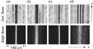
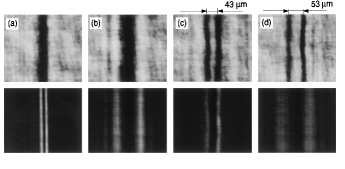
Figure 1: (Color Online) Formation of DB solitons in photorefractive crystals: the left four panels (adapted from Ref. [17]) showcase the evolution of an initial condition [panel (a)], upon propagation under linear evolution, leading to dispersion [panel (b)], nonlinear evolution of uncoupled components, again leading to breakup/dispersion [panel (d)], and under coupled nonlinear evolution [panel (c)]. A similar case example, but for two bright beams, is shown in the right four panels (adapted from Ref. [18]). The dark (bright) component is shown in the top (bottom) panel.

As discussed above, DB soliton states were first observed in pioneering experiments in optics [17, 18]; their key findings, summarized also in Fig. 1, were as follows. Experiments were performed in a photorefractive (strontium barium niobate) medium, with an input corresponding to a dark soliton (created through an optical mask) in one component, coupled to a bright soliton in the second component [panel (a) in the left of the figure]. For low intensity, i.e., for a linear evolution, both components underwent dispersion-induced broadening [panel (b)]. On the other hand, uncoupled nonlinear evolution [panel (d)] again resulted in dispersion of the bright component, since the corresponding structure was not effectively confined by the presence of the dark one. Only when the evolution is nonlinear and the two components are coupled [panel (c)], is it possible for the DB soliton state to persist. Similarly, for initial conditions conducive to a breakup into two DB waves (right four panels in Fig. 1), linear propagation, and uncoupled nonlinear propagation [panels (b) and (d)] do not lead to coherent states. Only the coupled nonlinear evolution [panel (c)] leads to a robust pair of DB solitons, i.e., a so-called “solitonic gluon” [18], or “soliton molecule”.

2.3 BEC experiments

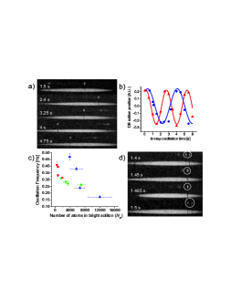
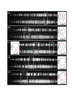
Figure 2: (Color Online) The left four panels (adapted from Ref. [32]), show: the oscillation of a DB soliton in a trapped BEC (a); the soliton position for different “masses” of the bright soliton (b); the oscillation frequency as a function of the bright soliton mass (c) and the collision of two DB solitons (d). The right panel (adapted from Ref. [33]) shows (transient) states bearing 2 (a), 3 (b), 4 (c), 5 (d) and even 6 (e) DB solitons.

In the context of BECs, DB solitons were first predicted and studied in binary BECs in Ref. [40]. While this theoretical work triggered a number of follow-up studies ramifying the original idea [3], arguably, it was the Hamburg experiment [30], and subsequently those at Pullman [31, 35, 32, 33, 36, 34] that put the topic in a fundamentally new perspective by revealing the experimental possibilities thereof. In particular, in Ref. [30] it was demonstrated that DB solitons can be created by a phase-imprinting technique in the two-component setting, and also showcased their robust oscillations in a quasi-1D parabolic trap. In turn, a different breed of experiments was introduced later, where both DB [31, 32, 33] and DD [35, 36] solitons were generated spontaneously via instability mechanisms in counterflow experiments: specifically, the condensates (composed of two distinct hyperfine states) were spatially separated and subsequently “slammed” against each other, leading to the spontaneous emergence of the coherent structures of interest.

Examples illustrating the above mentioned experimental possibilities and findings are shown in Figs. 2 and 3. In particular, Fig. 2 depicts robust oscillations of a DB soliton in a quasi-1D trap [left panel (a)]. The time-series of the wave center position [left panel (b)] allows to infer the oscillation frequency, as well as its dependence on the “mass” (number of atoms) of the bright component [left panel (c)]; this suggests that heavier solitons become slower, bearing an increasing period. In addition, collisions between two separately oscillating DB solitons are shown [left panel (d)]. The right set of panels depicts that states with two up to six DB solitons can (at least transiently) form during the complex evolution of the counterflow experiments. This again points to the idea of soliton molecules and progressively more elaborate states bearing multiple DB solitons.

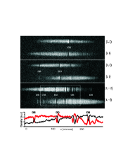
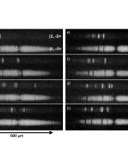
Figure 3: (Color Online) The left panels (adapted from Ref. [36]) depict different experimental snapshots of counterflow experiments of two different BEC components; the density profiles shown in the fourth panel correspond to a spatial region depicted in the third panel. The eight panels on the right (adapted from Ref. [34]) show progressively in time the interaction of a DB soliton with a Gaussian barrier: for a sufficiently high energy the wave is transmitted [panels (a-d)], while for a lower energy it is reflected [panels (e-h)].

Finally, Fig. 3 motivates some variants on the theme of DB solitons in BECs, by virtue of additional experiments [33, 34]. The left panel shows that in the counterflow experiments not only DB solitons but also DD ones are generated. The middle and right panels depict the interaction of a DB soliton with a potential barrier, induced by a Gaussian laser beam. When the barrier is shallow (or equivalently the wave bears sufficient energy to overcome the barrier), transmission through the barrier is observed (middle panel), while in the reverse scenario of a deep barrier (or insufficiently energetic DB solitons), near perfect reflection is realized (right panel).

3 Dark-Bright and Dark-Dark Solitons in 1D

3.1 The homogeneous setting

Motivated by these experimental results, we now turn to a theoretical study of the DB and DD solitons in the 1D setting. There, in the case of two components and in the absence of linear coupling, Eq. (1) becomes:

$$\begin{array}[]{rcl}i\partial_{t}\psi_{1}&=&-\frac{1}{2}\,\partial_{x}^{2}\psi_{1}+V(x)\psi_{1}+(|\psi_{1}|^{2}+|\psi_{2}|^{2}-\mu_{1})\psi_{1},\\[6.45831pt] i\partial_{t}\psi_{2}&=&-\frac{1}{2}\,\partial_{x}^{2}\psi_{2}+V(x)\psi_{2}+(|\psi_{1}|^{2}+|\psi_{2}|^{2}-\mu_{2})\psi_{2},\end{array}$$ (3)

where we have considered the Manakov limit with $g_{ij}=1$ [7]. This is motivated, e.g., by the physically relevant case of the ⁸⁷Rb BEC, where hyperfine states are characterized by almost equal coupling strengths [30, 31]. For $\mu_{1}=\mu_{2}=\mu$, and neglecting —to a first approximation— the confining potential, Eqs. (3) possess the following DB soliton solution:

$$\psi_{1}(x,t) = \sqrt{\mu}(\cos\phi\,\tanh\xi+i\sin\phi),$$ (4)

$$\psi_{2}(x,t) = \eta\,\mathop{\rm sech}\nolimits\xi\,\exp[ikx+i\theta(t)],$$ (5)

where $\xi=D(x-x_{0}(t))$, $\phi$ is the phase angle of the dark soliton, $\cos\phi$ and $\eta$ are the amplitudes of the dark and bright solitons, while $D$ and $x_{0}(t)$ describe the inverse width and the center position of the DB soliton. For this solution to be valid, $D^{2}=\mu\cos^{2}\phi-\eta^{2}$, the soliton velocity is given by $\dot{x}_{0}=k=D\tan\phi$, and phase $\theta(t)=(1/2)(D^{2}-k^{2})t+\theta_{0}$ (with $\theta_{0}={\rm const.}$).

A remarkable feature of the above Manakov system is its invariance under SU$(2)$ rotations, i.e., under the action of matrices of the form:

$$U=\left(\begin{array}[]{ccc}\alpha&-\beta^{*}\\ \beta&\alpha^{*}\end{array}\right),$$

with $|\alpha|^{2}+|\beta|^{2}=1$, for complex $\alpha,\beta$ (stars denote complex conjugation). For concreteness, limiting our considerations to the SO$(2)$ case [36], we choose $\alpha=\cos(\delta)$ and $\beta=\sin(\delta)$. Then, the respective (time-dependent) densities $n_{i}=|\psi_{i}|^{2}$ of the two components, upon rotation of a DB solution become:

$$n_{1} = \mu\cos^{2}(\delta)-(\mu\cos^{2}(\delta)\cos^{2}\phi-\eta^{2}\sin^{2}(\delta)){\mathop{\rm sech}\nolimits}^{2}\xi-\sqrt{\mu}\eta\sin(2\delta)\quad$$ (6)

$$\times \left\{\sin\phi\sin[kx+\theta(t)]+\cos\phi\cos[kx+\theta(t)]\tanh\xi\right\}{\mathop{\rm sech}\nolimits}\xi,$$

$$n_{2} = \mu\sin^{2}(\delta)-(\mu\sin^{2}(\delta)\cos^{2}\phi-\eta^{2}\cos^{2}(\delta)){\mathop{\rm sech}\nolimits}^{2}\xi+\sqrt{\mu}\eta\sin(2\delta)\quad$$ (7)

$$\times \left\{\sin\phi\sin[kx+\theta(t)]+\cos\phi\cos[kx+\theta(t)]\tanh\xi\right\}{\mathop{\rm sech}\nolimits}\xi.$$

There are three key features to discern within these complicated expressions. This DD soliton family contains the “standard” co-located DD solitons in the $\eta=0$ limit (i.e., in the absence of the bright component). Second, the DD solitons are generally asymmetric, unless $\delta=\pi/4$. Third, the time-dependence of phase $\theta(t)$ results in time-dependent density profiles, unless $\eta=0$; thus, DD solitons may feature time-dependent densities. For $\eta\neq 0$, the time-dependence is harmonic, with an oscillation frequency $\omega_{0}$ such that:

$$\frac{1}{2}k^{2}<\omega_{0}=\frac{1}{2}(k^{2}+D^{2})=\frac{1}{2}(\mu-\eta^{2}\sec^{2}\phi)<\frac{1}{2}\mu,$$ (8)

These important features highlighted above are illustrated in Fig. 4.

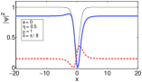
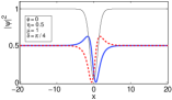
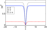
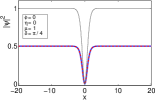
Figure 4: (Color Online) Profiles of non-co-located (for $\eta=0.5$; top panels), and co-located ($\eta=0$; bottom panels) DD solitons. For the left (right) panels, $\delta=\pi/8$ ($\delta=\pi/4$), so density profiles are asymmetric (symmetric). Thick solid (dashed) line represents the first (second) component and the thin solid line is the total density (adapted from Ref. [3]).

3.2 Dark-bright and dark-dark solitons in the trap.

We now turn to the case where a parabolic trapping potential is present. In this setting, the experimental findings depicted in Fig. 2 (see also Ref. [40]) illustrate that a DB soliton oscillates in the trap, following the dynamics of a classical harmonic oscillator. Such a “particle-like” oscillation of the DB soliton can be treated perturbatively [41, 42] in the Thomas-Fermi (TF) limit [20], where the wave can be considered as a Newtonian particle inside an effective potential.

To elaborate on this, we first recall that in the TF limit the ground state density of the first component (assumed to carry the dark soliton) is $|\psi_{1{\rm TF}}|^{2}=\max\{\mu-V(x),0\}$ [20]. Then, denoting by $u_{d}$ and $u_{b}$ the wavefunctions of the dark and bright soliton, we use $\psi_{1}\rightarrow\psi_{1{\rm TF}}u_{d}$ and $|\psi_{2}|^{2}\rightarrow\mu^{-1}|u_{b}|^{2}$, as well as $t\rightarrow\mu t$ and $x\rightarrow{\sqrt{\mu}}x$, and derive from Eq. (3) the system [41]:

$$\begin{array}[]{rcl}i\partial_{t}u_{d}+\frac{1}{2}\partial^{2}_{x}u_{d}-\left(|u_{d}|^{2}+|u_{b}|^{2}-1\right)u_{d}&=&R_{d},\\[6.45831pt] i\partial_{t}u_{b}+\frac{1}{2}\partial^{2}_{x}u_{b}-\left(|u_{b}|^{2}+|u_{d}|^{2}-\tilde{\mu}\right)u_{b}&=&R_{b},\end{array}$$ (9)

where we have assumed chemical potentials for the dark and bright solitons $\mu_{1}=\mu_{d}=\mu$ and $\mu_{2}=\mu_{b}=\mu+\Delta$ (with the difference being $\Delta<0$), so that $\tilde{\mu}=1+\Delta/\mu$. Finally, the perturbations $R_{d}$ and $R_{b}$ are given by:

$$R_{d} \equiv (2\mu^{2})^{-1}[2(1-|u_{d}|^{2})V(x)u_{d}+V^{\prime}(x)\partial_{x}u_{d}],$$ (10)

$$R_{b} \equiv \mu^{-2}[(1-|u_{d}|^{2})V(x)u_{b}].$$ (11)

We now assume adiabatic evolution of the DB soliton in the presence of the perturbations $R_{d,b}$, so that the soliton preserves its shape but its parameters become unknown functions of time, namely:

$$D^{2}(t)=\cos^{2}\phi(t)-\frac{1}{2}\chi D(t)\quad{\rm and}\quad\dot{x}_{0}(t)=D(t)\tan\phi(t).$$ (12)

Then, calculating the rate of change of the total energy of the system:

$$E=\frac{1}{2}\int_{-\infty}^{+\infty}|\partial_{x}u_{d}|^{2}+|\partial_{x}u_{b}|^{2}+(|u_{d}|^{2}+|u_{b}|^{2}-1)^{2}-2(\tilde{\mu}-1)|u_{b}|^{2}\,dx,$$ (13)

we obtain:

$$4\dot{D}D^{2}+\chi D\sec^{2}\phi(\dot{D}+D\dot{\phi}\tan\phi)=\frac{\cos\phi}{\mu^{2}}\left(\sin 2\phi-\chi D\sin\phi\right)V^{\prime}(x_{0}).$$ (14)

We thus derive the dynamical system of Eqs. (12) and (14), which possesses the fixed point: $x_{0,{\rm eq}}=0$, $\phi_{\rm eq}=0$, $D_{\rm eq}=\sqrt{1+\left(\frac{\chi}{4}\right)^{2}}-\frac{\chi}{4}$. Linearizing around it, and assuming a parabolic trap of strength $\Omega$, i.e., $V(x)=(1/2)\Omega^{2}x^{2}$, we find the equation of motion for the DB soliton center:

$$\ddot{x}_{0}=-\omega_{\rm osc}^{2}x_{0}\quad{\rm where}\quad\omega_{\rm osc}^{2}=\Omega^{2}\left(\frac{1}{2}-\frac{\chi}{8\sqrt{1+(\chi/4)^{2}}}\right).$$ (15)

Note that the oscillation frequency can also be derived via a Bogolyubov-de Gennes (BdG) analysis [20, 3] as follows. Denoting by $u_{d,b}^{(0)}$ the dark and bright components of a stationary DB soliton in the trap (cf. left panel of Fig. 5 for an example), we use the ansatz

$$u_{d}(x,t) = e^{-i\mu_{d}t}\left[u_{d}^{(0)}(x)+\epsilon\left(a(x)e^{\lambda t}+b^{\star}(x)e^{\lambda^{\star}t}\right)\right],$$ (16)

$$u_{b}(x,t) = e^{-i\mu_{b}t}\left[u_{b}^{(0)}(x)+\epsilon\left(c(x)e^{\lambda t}+d^{\star}(x)e^{\lambda^{\star}t}\right)\right],$$ (17)

where $(a,b,c,d)^{T}$ is the eigenvector of the perturbation and $\lambda$ is its corresponding eigenvalue. Substituting Eqs. (16)-(17) in the equations of motion, and linearizing in the small parameter $\epsilon$, we derive an eigenvalue problem for $[\lambda,(a,b,c,d)^{T}]$. The essence of the BdG analysis is that, once this problem is solved and $\lambda$ are found, if ${\rm Re}\{\lambda\}>0$ then the solution is unstable; else it is spectrally stable. The BdG analysis in our case reveals that the eigenvalues are imaginary, attesting to the DB soliton stability.

The middle and right panels of Fig. 5 show the dependence of the imaginary part of the lowest nonzero eigenvalue on the chemical potential of the dark and bright component, respectively. It is observed that the lowest nonzero eigenfrequency, associated with an internal mode (so-called anomalous mode [20, 3]) of the wave describing its oscillation in the trap, is in very good agreement with the theoretical prediction of Eq. (14).

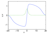
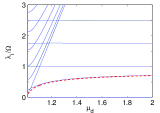
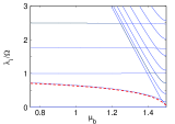
Figure 5: (Color Online) Left panel: a stationary DB soliton in a parabolic trap; solid blue (dashed green) line depicts the dark (bright) component. Middle and right panels: dependence of the eigenvalues (normalized to the trap strength) on the chemical potential of the dark and bright component, respectively, as obtained numerically via the BdG analysis. The lowest nonzero eigenfrequency is in very good agreement with the theoretical prediction (red dashed line) of Eq. (14) (adapted from Ref. [33]).

The analytical approach presented above is rather general in its nature: this energy balance methodology can be used to study the dynamics of coherent structures of different nature, and even different dimensionality, in Hamiltonian models in the presence of perturbations. On the other hand, it is relevant to remark that the SU$(2)$ and SO$(2)$ transformations are unaffected by the presence of the trap, and hence apply to the case of DD solitons with time-dependent density (so-called “beating DD solitons” [36]) as they do for the DB ones. Hence, the beating DD solitons have the same oscillation frequency [cf. Eq. (15)] as the DB ones [36]. Lastly, we note that the above BdG results for the 1D setting, indicate that the DB soliton is generally robust/spectrally stable; however, in the full 3D setting DB solitons turn out to be more prone to instabilities [32].

3.3 Multiple vector solitons and solitonic gluons

The next experimental aspect that we address is that of the emergence of bound states of multiple DB solitons. Such solitonic gluons (or “soliton molecules”) were observed first in optics [18] and also, more recently, in BEC experiments [33]. To provide an understanding for such states, we employ the variational approach of Ref. [33], and use the following ansatz for two equal-amplitude DB solitons traveling in opposite directions:

$$\!\!\!\!\!\!u_{d}(x,t) \!\!=\!\! \left(\cos\phi\tanh X_{-}+i\sin\phi\right)\left(\cos\phi\tanh X_{+}-i\sin\phi\right),$$ (18)

$$\!\!\!\!\!\!u_{b}(x,t) \!\!=\!\! \eta\,{\mathop{\rm sech}\nolimits}X_{-}\,e^{i\left[kx+\theta)+(\tilde{\mu}-1)t\right]}+\eta\,{\mathop{\rm sech}\nolimits}X_{+}\,e^{i\left[-kx+\theta)+(\tilde{\mu}-1)t\right]}\,e^{i\Delta\theta},\quad$$ (19)

where $X_{\pm}=D\left(x\pm x_{0}(t)\right)$, $2x_{0}$ is the relative distance between the two waves, and $\Delta\theta$ is the relative phase between the two bright components. Substituting the above ansatz into the energy of the system [cf. Eq. (13)], and considering low-velocity and well-separated ($x_{0}\gg 1$) solitons, it is found that the energy of the system assumes the form:

$$E=2E_{1}+E_{\rm DD}+E_{\rm BB}+2E_{\rm DB},$$ (20)

i.e., the energy consists of twice the energy $E_{1}$ of one DB soliton, the interaction energies $E_{DD}$ and $E_{BB}$ between the two dark and the two bright solitons, and twice the cross interaction energy $E_{DB}$ of the dark component of one soliton with the bright of the other (cf. Ref. [33] for expressions of these energies). We can then find the evolution of the soliton parameters from the energy conservation, $dE/dt=0$, as in the previous case of the single DB soliton in the trap. This way, for low-velocity, almost black solitons, energy conservation leads to the following equation for the soliton center:

$$\ddot{x}_{0}=F_{\rm int}\equiv F_{\rm DD}+F_{\rm BB}+2F_{\rm DB},$$ (21)

where we have used the same notation for the respective interaction forces. To the leading order of approximation, it can be found that [33]:

$$F_{\rm BB}\propto{\rm e}^{-2D_{\rm eq}x_{0}}\cos(\Delta\theta),~{}~{}F_{\rm DD}\propto{\rm e}^{-4D_{\rm eq}x_{0}},~{}~{}F_{\rm DB}\propto{\rm e}^{-2D_{\rm eq}x_{0}}\cos(\Delta\theta).$$ (22)

The key feature here is that while the DD interaction is always repulsive, the BB and DB ones depend on the relative phase $\Delta\theta$ between the bright components. In particular, if $\Delta\theta=0$ then the BB interaction is also repulsive, rendering impossible a stationary “molecular” state. However, if $\Delta\theta=\pi$ (as found in Ref. [18]), then the repulsive nature of the DD interaction dominates at short distances, while the attractive nature of the BB interaction at long ones, yielding the potential for a “bound state”, the solitonic gluon.

The above analysis allows for the identification of this state numerically (even in the absence of a trap), and also provides the dependence of the center of the solitonic gluon on, e.g., the bright component chemical potential. Equally importantly, linearization around the equilibrium position $x_{\rm eq}$ (i.e., the distance between the constituent DB solitons forming the stationary solitonic gluon) suggests the existence of an internal mode of the two DB solitons, involving their out-of-phase oscillation with a frequency $\omega_{0}^{2}=-\frac{\partial F_{\rm int}}{\partial x_{0}}\big{|}_{x_{0}=x_{\rm eq}}$. These predictions are illustrated in Fig. 6.

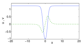
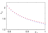
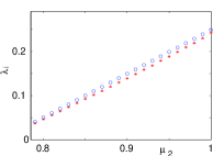
Figure 6: (Color Online) The dark (solid blue line) and bright (dashed green line) components of a solitonic gluon in the homogeneous case (left panel). The equilibrium distance between two DB solitons (middle panel) and the out-of-phase oscillation frequency (right panel) as functions of the bright component chemical potential; red stars denote the theoretical prediction and blue circles the numerical result (adapted from Ref. [33]).

These molecular states can be generalized in the presence of a trap: in this case, the equation of motion for the center $x_{0}$ of the solitonic gluon involves not only the pairwise interaction force $F_{\rm int}$, but also the restoring force of the trap $F_{\rm tr}$, inducing an in-trap oscillation with a frequency $\omega_{\rm osc}$ [cf. Eq. (15)]. Hence, the equation of motion for $x_{0}$ reads:

$$\ddot{x}_{0}=F_{\rm tr}+F_{\rm int}.$$ (23)

Thus, in this setting, a molecular state exists even when the two DB solitons are in-phase, because their DD and BB (and DB) repulsion is counterbalanced by $F_{\rm tr}$. An additional consequence is that, inside the trap, a pair of DB solitons will bear two, rather than one, internal modes. The lowest one, pertains to their in-phase oscillation, characterized by the frequency $\omega_{\rm osc}$; the other internal mode corresponds to their out-of-phase motion, characterized by the frequency $\omega_{1}^{2}=\omega_{0}^{2}+\omega_{\rm osc}^{2}$.

Motivated by the observation of multi-DB-solitons (cf. right panel of Fig. 2), we may also consider “lattices” of such states. In particular, lattices of DB solitons, with out- or in-phase bright neighbors respectively read [42]:

$$u_{d} = A_{1}~{}{\rm sn}(bx,k),\quad u_{b}=A_{2}~{}{\rm cn}(bx,k),$$ (24)

$$u_{d} = A_{1}~{}{\rm sn}(bx,k),\quad u_{b}=A_{2}~{}{\rm dn}(bx,k),$$ (25)

where suitable (explicit) conditions connect amplitudes, $A_{1},~{}A_{2}$, and width as well as inter-soliton separation parameters $b$ and $k$. Such solutions exist for general nonlinearity coefficients $g_{ij}$, and can be numerically found even well beyond the regime of validity of the analytical solutions [42].

Furthermore, in Ref. [43], it was found that the lattice states can still be described via the above particle model characterizing the pairwise interactions between the nearest-neighbor DB solitons. Moreover, a notion of “kinetic temperature” was introduced, depending on the solitons’ initial kinetic energy. In that light, a (gradual) transition of the dynamics of a large number of solitons could be identified as follows. When the kinetic energy (and hence the kinetic temperature) of the system was low, the array of the DB solitons behaved as a crystal. As the kinetic temperature was increased, the DBs progressively demonstrated a more gaseous behavior with a large number of collision events. Intriguingly, these also included an exchange of mass between the bright components, rendering the particle description less accurate in this limit. This is a topic worthwhile of further exploration.

4 Variations on the theme

We now turn to a number of case examples in which variants of the standard homogeneous or trapped DB solitons are of relevance/interest.

4.1 The case of unequal masses

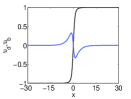
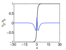
Figure 7: (Color Online) Excited states of bright solitons trapped by the dark soliton for $D<1$. Left, middle and right panels show, respectively, the first, the second (for $D<1/3$), and the third (for $D<1/6$) excited state. The dark and bright component profiles are depicted by black and blue lines, respectively (adapted from Ref. [47]).

Motivated by studies of spin-orbit coupled BECs [44, 45], it was recently shown [46] that pertinent GPEs can be reduced to an effective Manakov-type system but with “unequal masses” (i.e., unequal dispersion coefficients) among the two components of Eq. (3). Assuming that $D$ is the mass ratio of dark and bright components, and seeking stationary solutions of the GPEs (3) of the form $\psi_{1,2}=\upsilon_{d,b}(x)\exp(-i\mu_{d,b}t)$, we obtain the system:

$$\begin{array}[]{rcl}\mu_{d}\,\upsilon_{d}&=&-\frac{1}{2}\left(\upsilon_{d}\right)^{\prime\prime}+\left(\upsilon_{d}^{2}+\upsilon_{b}^{2}\right)\upsilon_{d}+V(x)\,\upsilon_{d},\\[4.30554pt] \mu_{b}\,\upsilon_{b}&=&-\frac{D}{2}\left(\upsilon_{b}\right)^{\prime\prime}+\left(\upsilon_{d}^{2}+\upsilon_{b}^{2}\right)\upsilon_{b}+V(x)\,\upsilon_{b}.\end{array}$$ (26)

The existence of DB solitons can be explored upon realizing that the dark soliton $u_{d}(x)=\sqrt{\mu_{d}}\tanh\left(\sqrt{\mu_{d}}x\right)$ [for $V(x)=0$] acts as an effective potential for the bright component [47]. This way, linearization of Eq. (26) for a small bright component gives rise to the eigenvalue problem:

$$\begin{array}[]{c}\mathcal{L}\,\upsilon_{b}=\lambda\,\upsilon_{b}\quad{\rm with}\quad{\mathcal{L}=\frac{D}{2}}\frac{d^{2}}{dx^{2}}{+\mu_{d}\,\mathrm{sech}^{2}\left(\sqrt{\mu_{d}}x\right)},\end{array}$$ (27)

where $\lambda=\mu_{d}-\mu_{b}$, while the Schrödinger operator $\mathcal{L}$ corresponds to the Pöschl-Teller potential, known from quantum mechanics [48]. Equation (27) supports bound states for integers $n$ satisfying $D<D_{\mathrm{crit}}^{(n)}=\frac{2}{n\left(1+n\right)}$. Hence, a fundamental (bound) state of the bright component, pertaining to the DB soliton, always exists. Furthermore, for $D<1$ (for $n=1$), it is also possible for the dark component to trap a first excited state in the bright one (i.e., a two-bright-soliton anti-phase pair). For $D<1/3$, it will be possible to trap a second excited state, and so on. Examples of such states, which were identified in Ref. [47], are shown in Fig. 7.

4.2 Dissipative dynamics under the action of thermal effects

Dissipative effects, induced by the interaction of the BEC with the thermal cloud, can be studied in the framework of the so-called dissipative GPE model [49]. In the two-component setting, this model arises from Eq. (3) upon the substitution $i\partial_{t}\psi_{1,2}\rightarrow(i-\gamma_{1,2})\partial_{t}\psi_{1,2}$ [50], where parameters $\gamma_{1,2}$ depend on temperature [51]. The dissipative GPE system describes phenomenologically, via the presence of losses, the transfer of atoms from the condensate to the thermal cloud. The dissipative dynamics of DB solitons in this setting can be studied upon generalizing the methodology of Sec. 3.2. This way, it is possible to derive an equation for motion for the DB soliton center, of the form: $\ddot{x}_{0}-a\,\dot{x}_{0}+\omega_{\rm osc}^{2}\,x_{0}=0$ [50], where

$$a=\frac{2}{3}\mu\left(\gamma_{1}-\frac{1}{8}\chi^{2}\gamma_{2}\right)+\frac{1}{6}\mu\left(\gamma_{2}-\gamma_{1}+\frac{1}{8}\chi^{2}\gamma_{2}\right)\frac{\chi}{\sqrt{1+(\chi/4)^{2}}}.$$ (28)

The generic positivity of parameter $a$ suggests that the newly introduced term, $-a\dot{x}_{0}$, represents an effective anti-damping. This term characterizes the interaction of the DB soliton with the thermal cloud. It results in the acceleration of the soliton toward the velocity of sound, i.e., the dark component becomes continuously grayer and, eventually, the wave transforms to the ground state of the BEC. A similar situation, in addition to their internal mode motion, is encountered in the case of multiple DB solitons. The accuracy of this effective particle picture in capturing the anti-damped dynamics is shown in Fig. 8.

It is important to note that, although this dynamics is similar to that of dark solitons in single BECs [51], the analysis of Ref. [50] reveals that the effect of the bright (“filling”) component is to partially stabilize dark solitons against temperature-induced dissipation, thus providing longer lifetimes.

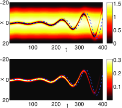
Figure 8: (Color Online) Examples of the anti-damped dynamics of one (left panels) and two (right panels) DB solitons; top (bottom) panels depict the dark (bright) component. Dashed (blue) lines depict the analytical predictions (adapted from Ref. [50]).

4.3 Dark-bright solitons in spinor condensates

We now proceed with a case involving more than two components, and study, more specifically, spinor BECs. The latter, have been realized by employing optical trapping techniques, which allow for the confinement of atoms regardless of their spin hyperfine state; thus, spinor BECs formed by atoms with spin $F$, are described by a macroscopic wave function with $2F+1$ components [20]. It is relevant to highlight that spinor BECs give rise to various phenomena that are not present in single-component BECs, including formation of spin domains, spin textures, topological states, and others [25, 26].

Here, we only consider a case example, namely a quasi-1D spinor $F=1$ BEC, described by the following dimensionless mean-field model [52, 53]:

$$i\partial_{t}\psi_{\pm 1} = H_{0}\psi_{\pm 1}+\delta\left[(|\psi_{\pm 1}|^{2}+|\psi_{0}|^{2}-|\psi_{\mp 1}|^{2})\psi_{\pm 1}+\psi_{0}^{2}\psi_{\mp 1}^{\ast}\right],$$ (29)

$$i\partial_{t}\psi_{0} = H_{0}\psi_{0}+\delta\left[(|\psi_{-1}|^{2}+|\psi_{+1}|^{2})\psi_{0}+2\psi_{-1}\psi_{0}^{\ast}\psi_{+1}\right].$$ (30)

Here, the components $\psi_{0,\pm 1}$ correspond to the three values of the vertical spin component $m_{F}=0,\pm 1$, while $H_{0}\equiv-(1/2)\partial_{x}^{2}+V(x)+|\psi_{-1}|^{2}+|\psi_{0}|^{2}+|\psi_{+1}|^{2}$, and $\delta$ is the ratio of the strengths of the spin-dependent and spin-independent interatomic interactions. Note that $\delta$ is positive (negative) for polar (ferromagnetic) spinor BECs as, e.g., in the case of ²³Na (⁸⁷Rb) atoms, where this parameter takes the value $\delta=+3.14\times 10^{-2}$ ($\delta=-4.66\times 10^{-3}$).

As shown in Ref. [52], for $\delta>0$ the background state (on which a dark soliton may be supported) is modulationally stable; this suggests that DB soliton solutions of Eqs. (29)-(30) may be possible. Indeed, in Ref. [53], exploiting the smallness of $\delta$, a multiscale expansion method was used [for $V(x)=0$] to show that such states do exist, and assume the following form:

$$\begin{array}[]{rcl}\psi_{\pm 1}&=&\sqrt{\left(\mu/2\right)+\delta\rho(X,T)}\exp\left[-i\mu t+(2i\delta/\mu)\int\rho(X)dX\right],\\[4.30554pt] \psi_{0}&=&\delta^{3/4}q(X,T)\exp(-i\mu t),\end{array}$$ (31)

where $\mu$ is the chemical potential, $X=\sqrt{\delta}(x-\sqrt{\mu}t)$ and $T=\delta t$ are stretched variables, while functions the $\rho(X,T)$ and $q(X,T)$ obey the following system:

$$\begin{array}[]{c}\partial_{T}\rho=-\frac{1}{2}\sqrt{\mu}\partial_{X}\left(|q|^{2}\right),\quad i\partial_{T}q+\frac{1}{2}\partial_{X}^{2}q-2\rho q=0.\end{array}$$ (32)

The above is the Yajima-Oikawa (YO) system, which was originally derived to describe the interaction of Langmuir and sound waves in plasmas [54]. This system is completely integrable, and possesses soliton solutions of the form $\rho\propto-{\rm sech}^{2}(k_{s}X-\omega_{s}T)$ and $q\propto{\rm sech}(k_{s}X-\omega_{s}T)$, where $k_{s},~{}\omega_{s}$ are constants. These expressions, when substituted into Eq. (31), give rise to approximate dark-dark-bright (for the $m_{F}=+1,-1,0$ spin components) solitons, while a similar analysis can also lead to bright-bright-dark ones. As shown in Ref. [53], these small-amplitude structures persist for large amplitudes and, in the presence of a parabolic trap, they perform harmonic oscillations, in a way reminiscent of the two-component case.

We note in passing that similar asymptotic reductions of other multi-component GPEs, have been used to construct vector soliton solutions described by integrable systems, such as the Yajima-Oikawa (already mentioned above) and the Davey-Stewartson (DS) ones [55], the Mel’nikov system [55, 56], and a coupled Korteweg-de Vries (KdV) equations system [57].

4.4 Vector solitons in higher-dimensions

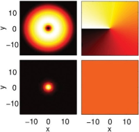
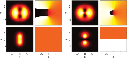
Figure 9: (Color Online) The left panel quartet shows a single vortex-bright solitary wave, while the middle and right quartets show, respectively, dipoles thereof, with in-phase or out-of-phase bright components (adapted from Ref. [59]). Top (bottom) panels depict the vortex (bright) component, while left (right) panels depict densities (phases).

The concept that one component acts as a potential to trap the other, is one that transcends dimensionality. Indeed, considering the 2D variant of Eq. (3), a vortex (which is a prototypical coherent structure in 2D repulsive BECs [3]) in component $\psi_{1}$ can play the role of a potential trapping a bright soliton in component $\psi_{2}$. A case example of a vortex-bright soliton is shown in Fig. 9. Note that these structures bear different names in different communities, such as vortex-bright solitons [58, 59], half-quantum vortices [60] or baby Skyrmions [61]. Various studies have been devoted to the stability [62, 58] and dynamics [58, 60] of these structures. Moreover, it was found that they feature intriguing interactions that decay as $1/r^{3}$ [60]. They also allow much of the phenomenology discussed previously, including their potential to form molecular states with out-of-phase and in-phase bright solitons in the presence of the trap (cf. middle and right panels of Fig. 9, as well as the work of Ref. [59]).

Another quasi-2D state, is the ring DB soliton explored in Ref. [63]. The matter-wave ring dark soliton (RDS), introduced in Ref. [64], is a 2D radial generalization of the dark soliton which, however, is generically unstable due to breakup into vortex-antivortex polygonal structures (squares, hexagons, etc.). Nevertheless, in the two-component setting, the RDS in one component can form an effective potential that supports a bright ring soliton structure in the other component. As found in Ref. [63], although the presence of the bright component weakens the instability of the RDS, it is not possible to eliminate it completely. Nevertheless, the instability gives rise to states of interest in their own right, such as vortex-bright polygons and DB soliton stripes.

4.5 The double-well potential perspective

Lastly, as regards the variants considered herein, when two dark solitons (or two vortices) trap two bright ones, one can also view the relevant molecule under a different prism, namely that of topological states in the first component forming an effective double-well potential for the second one. This perspective was used in the cases of DB solitons in 1D [65], and vortex-bright solitons in 2D [59]. Importantly, given their genuine topological nature, vortices form, in a sense, a more “robust” double-well. Namely, while this approach neglects the back-action of the bright components on the dark ones (i.e., this is a “soft” potential, rather than a hard, externally imposed, one), this feedback mechanism is present and is more significant in 1D than in 2D. Nevertheless, in both settings, this approach enabled the observation of features associated with double-well potentials, such as symmetry-breaking bifurcations, Josephson oscillations, and so-called $\pi$-states emerging from the bifurcations (see Ref. [66] and references therein).

5 Conclusions & Outlook

In this review, we examined coherent structures arising in coupled defocusing nonlinear Schrödinger equations, especially so in the vicinity of the so-called Manakov limit of equal self- and cross-interactions. There (but also away from that limit), a fundamental concept emerges, namely that a “dark structure” in one component (be it a dark soliton in 1D or a vortex in 2D) acts as a potential well for the second component. This enables the confinement therein of a bright soliton and the formation of “dark-bright states”. These states also persist in the presence of external (e.g., parabolic) potentials, wherein they oscillate as Newtonian particles. Molecular states involving multiple dark-bright waves may exist for appropriate phase difference between the bright components in the homogeneous setting (solitonic gluons), and in the presence of external traps. Moreover, rotated versions of such dark-bright solitons also emerge in experiments, in the form of the so-called beating dark-dark solitons.

Additionally, variations on these themes were recognized and explored. The dark structure potential well was, for instance, recognized as possibly trapping higher-excited states. Another possibility concerned the prototypical characterization of the thermal-induced dissipation, that leads to anti-damping and eventual expulsion of dark-bright solitons from trapped atomic condensates. The relevance of higher-component settings bearing spinor analogues of the considered states was also discussed. Here, dark-dark-bright, or bright-bright-dark states were found via a multiscale asymptotic analysis. Another equally important and experimentally tractable generalization arose in higher-dimensional settings, where vortex-bright solitons, as well as dark-bright ring solitons were presented. Finally, molecular states bearing two (or more) dark entities were also perceived as double (or, respectively, multi-) well potentials, thus enabling related phenomena.

We hope that it is clear that the above ideas and paradigms are powerful and broad beyond any one of the particular examples used, and could lead to a wealth of future possibilities and explorations, both in theory and experiments. As a small sample of the questions that merit future consideration, we pose the following. Is it possible to identify dark-bright solitonic states (and their variants) in the context of the intensely studied recently spin-orbit coupled BECs ? Can a quantitative understanding of the scattering of vector solitons off of Gaussian barriers (or wells) be achieved ? Can we trap higher-excited states in higher-dimensional settings (radial and/or azimuthally dependent ones) ? Can an analogue of dark-dark states be observed in higher-dimensions ? What are the implications of these ideas in three-dimensional settings ? All these are important open questions, a number of which are under active current consideration and, we expect, will lead to numerous discoveries ahead…

References

References

- [1] C. Sulem and P.L. Sulem, The Nonlinear Schrödinger Equation, Springer-Verlag (New York, 1999).
- [2] M.J. Ablowitz, B. Prinari, and A.D. Trubatch, Discrete and Continuous Nonlinear Schrödinger Systems, Cambridge University Press (Cambridge, 2004).
- [3] P.G. Kevrekidis, D.J. Frantzeskakis, and R. Carretero-González, The Defocusing Nonlinear Schrödinger Equation, SIAM (Philadelphia, 2015).
- [4] E. Infeld, G. Rowlands, Nonlinear Waves, Solitons and Chaos, Cambridge University Press (Cambridge, 1990).
- [5] Yu.S. Kivshar and G.P. Agrawal, Optical Solitons: from fibers to photonic crystals, Academic Press (San Diego, 2003).
- [6] P.G. Kevrekidis, D.J. Frantzeskakis, and R. Carretero-González (Eds.), Emergent Nonlinear Phenomena in Bose-Einstein Condensates: Theory and Experiment Springer-Verlag (Heidelberg, 2008).
- [7] S.V. Manakov, Sov. Phys. JETP, 38 (1973) 248–253.
- [8] V.E. Zakharov and S.V. Manakov, Sov. Phys. JETP, 42 (1976) 842–850
- [9] V.E. Zakharov and E.I. Schulman, Physica D, 4 (1982) 270–274.
- [10] D.N. Christodoulides, Phys. Lett. A, 132 (1988) 451–452.
- [11] V.V. Afanasyev, Yu.S. Kivshar, V.V. Konotop, and V.N. Serkin, Opt. Lett., 14 (1989) 805–807.
- [12] Yu.S. Kivshar and S.K. Turitsyn, Opt. Lett., 18 (1993) 337–339.
- [13] R. Radhakrishnan and M. Lakshmanan, J. Phys. A: Math. Gen., 28 (1995) 2683–2692.
- [14] A.V. Buryak, Yu.S. Kivshar, and D.F. Parker, Phys. Lett. A, 215 (1996) 57–62.
- [15] A.P. Sheppard and Yu.S. Kivshar, Phys. Rev. E, 55 (1997) 4773–4782.
- [16] Q.-H. Park and H.J. Shin, Phys. Rev. E, 61 (2000) 3093–3106.
- [17] Z. Chen, M. Segev, T.H. Coskun, D.N. Christodoulides, and Yu.S. Kivshar, J. Opt. Soc. Am. B, 14 (1997) 3066–3077.
- [18] E.A. Ostrovskaya, Yu.S. Kivshar, Z. Chen, and M. Segev, Opt. Lett., 24 (1999) 327–329.
- [19] B.A. Malomed, Prog. Optics, 43 (2002) 71–194.
- [20] L.P. Pitaevskii and S. Stringari, Bose-Einstein Condensation. Oxford University Press (Oxford, 2003).
- [21] V.S. Bagnato, D.J. Frantzeskakis, P.G. Kevrekidis, B.A. Malomed, and D. Mihalache, Rom. Rep. Phys., 67 (2015) 5–50.
- [22] D.S. Hall, M.R. Matthews, J.R. Ensher, C.E. Wieman, and E.A. Cornell, Phys. Rev. Lett., 81 (1998) 1539–1542.
- [23] D.M. Stamper-Kurn, M.R. Andrews, A.P. Chikkatur, S. Inouye, H.-J. Miesner, J. Stenger, and W. Ketterle, Phys. Rev. Lett., 80 (1998) 2027–2030.
- [24] J. Stenger, S. Inouye, D.M. Stamper-Kurn, H.-J. Miesner, A.P. Chikkatur, and W. Ketterle, Nature, 396 (1998) 345–348.
- [25] Y. Kawaguchi and M. Ueda, Phys. Rep., 520 (2012) 253–381.
- [26] D.M. Stamper-Kurn and M. Ueda, Rev. Mod. Phys., 85 (2013) 1191–1244.
- [27] R.J. Ballagh, K. Burnett, and T.F. Scott, Phys. Rev. Lett., 78 (1997) 1607–1611.
- [28] V.P. Mineev, Sov. Phys. JETP, 40 (1974) 132–136.
- [29] M. Trippenbach, K. Goral, K. Rzazewski, B.A. Malomed, and Y.B. Band, J. Phys. B, 33 (2000) 4017–4031.
- [30] C. Becker, S. Stellmer, P. Soltan-Panahi, S. Dörscher, M. Baumert, E.-M. Richter, J. Kronjäger, K. Bongs, and K. Sengstock, Nature Phys., 4 (2008) 496–501.
- [31] C. Hamner, J.J. Chang, P. Engels, and M.A. Hoefer, Phys. Rev. Lett., 106 (2011) 065302.
- [32] S. Middelkamp, J.J. Chang, C. Hamner, R. Carretero-González, P.G. Kevrekidis, V. Achilleos, D.J. Frantzeskakis, P. Schmelcher, and P. Engels, Phys. Lett. A, 375 (2011) 642–646.
- [33] D. Yan, J.J. Chang, C. Hamner, P.G. Kevrekidis, P. Engels, V. Achilleos, D.J. Frantzeskakis, R. Carretero-González, and P. Schmelcher, Phys. Rev. A, 84 (2011) 053630.
- [34] A. Álvarez, J. Cuevas, F.R. Romero, C. Hamner, J.J. Chang, P. Engels, P.G. Kevrekidis, and D.J. Frantzeskakis, J. Phys. B, 46 (2013) 065302.
- [35] M.A. Hoefer, J.J. Chang, C. Hamner, and P. Engels, Phys. Rev. A, 84 (2011) 041605(R).
- [36] D. Yan, J.J. Chang, C. Hamner, M. Hoefer, P.G. Kevrekidis, P. Engels, V. Achilleos, D.J. Frantzeskakis, and J. Cuevas, J. Phys. B: At. Mol. Opt. Phys., 45 (2012) 115301.
- [37] P.G. Kevrekidis, H.E. Nistazakis, D.J. Frantzeskakis, B.A. Malomed, and R. Carretero-González, Eur. Phys. J. D, 28 (2004) 181–185.
- [38] H. Susanto, P.G. Kevrekidis, R. Carretero-González, B.A. Malomed, D.J. Frantzeskakis, and A.R. Bishop, Phys. Rev. A, 75 (2007) 055601.
- [39] K. Kasamatsu and M. Tsubota, Phys. Rev. A, 74 (2006) 013617.
- [40] Th. Busch and J.R. Anglin, Phys. Rev. Lett., 87 (2001) 010401.
- [41] V. Achilleos, P.G. Kevrekidis, V.M. Rothos, and D.J. Frantzeskakis, Phys. Rev. A, 84 (2011) 053626.
- [42] D. Yan, F. Tsitoura, P.G. Kevrekidis, and D.J. Frantzeskakis, Phys. Rev. A, 91 (2015) 023619.
- [43] Wenlong Wang and P. G. Kevrekidis, Phys. Rev. E, 91 (2015) 032905.
- [44] J. Dalibard, F. Gerbier, G. Juzeliunas, and P. Öhberg, Rev. Mod. Phys. 83 (2011) 1523–1543.
- [45] V. Galitski and I.B. Spielman, Nature 494 (2013) 49–54.
- [46] V. Achilleos, D. J. Frantzeskakis, and P.G. Kevrekidis, Phys. Rev. A, 89 (2014) 033636.
- [47] E.G. Charalampidis, P.G. Kevrekidis, D.J. Frantzeskakis, and B.A. Malomed, Phys. Rev. E, 91 (2015) 012924.
- [48] L.D. Landau and E.M. Lifshitz, Quantum Mechanics, Nauka (Moscow, 1989).
- [49] L.P. Pitaevskii, Sov. Phys. JETP, 8 (1959) 282–287.
- [50] V. Achilleos, D. Yan, P.G. Kevrekidis, and D.J. Frantzeskakis, New J. Phys., 14 (2012) 055006.
- [51] S.P. Cockburn, H.E. Nistazakis, T.P. Horikis, P.G. Kevrekidis, N.P. Proukakis, and D.J. Frantzeskakis, Phys. Rev. Lett., 104 (2010) 174101.
- [52] N.P. Robins, W. Zhang, E.A. Ostrovskaya, and Yu.S. Kivshar, Phys. Rev. A, 64 (2001) 021601(R).
- [53] H.E. Nistazakis, D.J. Frantzeskakis, P.G. Kevrekidis, B.A. Malomed, and R. Carretero-González, Phys. Rev. A, 77 (2008) 033612.
- [54] N. Yajima and M. Oikawa, Prog. Theor. Phys. 56 (1976) 1719–1739.
- [55] M. Aguero, D.J. Frantzeskakis, and P.G. Kevrekidis, J. Phys. A: Math. Gen., 39 (2006) 7705–7718.
- [56] F. Tsitoura, V. Achilleos, B.A. Malomed, D. Yan, P.G. Kevrekidis, and D.J. Frantzeskakis, Phys. Rev. A 87, 063624 (2013).
- [57] V.A. Brazhnyi and V.V. Konotop, Phys. Rev. E, 72 (2005) 026616.
- [58] K.J.H. Law, P.G. Kevrekidis, and L.S. Tuckerman, Phys. Rev. Lett., 105 (2010) 160405.
- [59] M. Pola, J. Stockhofe, P. Schmelcher, and P.G. Kevrekidis, Phys. Rev. A, 86 (2012) 053601.
- [60] M. Eto, K. Kasamatsu, M. Nitta, H. Takeuchi, and M. Tsubota, Phys. Rev. A, 83 (2011) 063603.
- [61] R.A. Battye, N.R. Cooper, and P.M. Sutcliffe, Phys. Rev. Lett., 88 (2002) 080401.
- [62] D.V. Skryabin, Phys. Rev. A, 63 (2001) 013602.
- [63] J. Stockhofe, P.G. Kevrekidis, D.J. Frantzeskakis, and P. Schmelcher, J. Phys. B, 44 (2011) 191003.
- [64] G. Theocharis, D.J. Frantzeskakis, P.G. Kevrekidis, B.A. Malomed and Yu.S. Kivshar, Phys. Rev. Lett., 90 (2003) 120403.
- [65] E.T. Karamatskos, J. Stockhofe, P.G. Kevrekidis, and P. Schmelcher, Phys. Rev. A, 91 (2015) 043637.
- [66] B.A. Malomed, Spontaneous Symmetry Breaking, Self-Trapping and Josephson Oscillations, Springer-Verlag (Berlin, 2013).