Axion phenomenology and $\theta$-dependence from $N_{f}=2+1$ lattice QCD

Abstract

We investigate the topological properties of $N_{f}=2+1$ QCD with physical quark masses, both at zero and finite temperature. We adopt stout improved staggered fermions and explore a range of lattice spacings $a\sim 0.05-0.12$ fm. At zero temperature we estimate both finite size and finite cut-off effects, comparing our continuum extrapolated results for the topological susceptibility $\chi$ with predictions from chiral perturbation theory. At finite temperature, we explore a region going from $T_{c}$ up to around $4\,T_{c}$, where we provide continuum extrapolated results for the topological susceptibility and for the fourth moment of the topological charge distribution. While the latter converges to the dilute instanton gas prediction the former differs strongly both in the size and in the temperature dependence. This results in a shift of the axion dark matter window of almost one order of magnitude with respect to the instanton computation.

1 Introduction

Axions are among the most interesting candidates for physics beyond the Standard Model. Their existence has been advocated long ago Peccei:1977hh ; Peccei:1977ur ; Wilczek:1977pj ; Weinberg:1977ma as a solution to the so-called strong-CP problem through the Peccei-Quinn (PQ) mechanism. It was soon realized that they could also explain the observed dark matter abundance of the visible Universe Preskill:1982cy ; Abbott:1982af ; Dine:1982ah . However, a reliable computation of the axion relic density requires a quantitative estimate of the parameters entering the effective potential of the axion field, in particular its mass and self-couplings as a function of the temperature $T$ of the thermal bath.

The purpose of this study is to obtain predictions from the numerical simulations of Quantum Chromodynamics (QCD) on a lattice. Our results, which are summarized at the end of this section, suggest a possible shift of the axion dark matter window by almost one order of magnitude with respect to instanton computations. This shift is a consequence of the much slower decrease of the axion mass with the temperature in comparison to the dilute instanton gas prediction. Our present simulations are however limited to a range of temperatures not exceeding 600 MeV: the main obstruction is represented by the freezing of the topological modes on fine lattices, which afflicts present lattice QCD algorithms. For a more complete understanding of axion dynamics at finite $T$, in the future a major effort must be undertaken to reach higher temperatures.

1.1 General framework

Given the strong bounds on its couplings, the axion field can be safely treated as a non-dynamical external field. Its potential is completely determined by the dependence of the QCD partition function on the $\theta$-angle, which enters the pure gauge part of the QCD Euclidean Lagrangian as

$$\mathcal{L}_{\theta}=\frac{1}{4}F_{\mu\nu}^{a}(x)F_{\mu\nu}^{a}(x)-i\theta q(x),$$ (1)

where

$$q(x)=\frac{g^{2}}{64\pi^{2}}\epsilon_{\mu\nu\rho\sigma}F_{\mu\nu}^{a}(x)F_{\rho\sigma}^{a}(x)$$ (2)

is the topological charge density. The $\theta$-dependent part of the free energy density can be parametrized as follows

$$\mathcal{F}(\theta,T)\equiv F(\theta,T)-F(0,T)={1\over 2}\chi(T)\theta^{2}s(\theta,T)$$ (3)

where $\chi(T)$ is the topological susceptibility at $\theta=0$,

$$\chi=\int d^{4}x\langle q(x)q(0)\rangle_{\theta=0}={\langle Q^{2}\rangle_{\theta=0}\over{\cal V}}$$ (4)

($Q=\int d^{4}x\,q(x)$ is the global topological charge and $\mathcal{V}=V/T$), while $s(\theta,T)$ is a dimensionless even function of $\theta$ such that $s(0,T)=1$. The quadratic term in $\theta$, $\chi(T)$, is proportional to the axion mass, while non-linear corrections in $\theta^{2}$, contained in $s(\theta,T)$, provide information about axion interactions. In particular, assuming analyticity around $\theta=0$, $s(\theta,T)$ can be expanded as follows Vicari:2008jw

$$s(\theta,T)=1+b_{2}(T)\theta^{2}+b_{4}(T)\theta^{4}+\cdots,$$ (5)

where the coefficients $b_{n}$ are proportional to the cumulants of the topological charge distribution. For instance $b_{2}$, which is related to quartic interactions terms in the axion potential, can be expressed as

$$b_{2}=-\frac{\langle Q^{4}\rangle_{\theta=0}-3\langle Q^{2}\rangle^{2}_{\theta=0}}{12\langle Q^{2}\rangle_{\theta=0}}\,.$$ (6)

The function ${\cal F}(\theta,T)$, related to the topological properties of QCD, is of non-perturbative nature and hence not easy to predict reliably with analytic methods. This is possible only in some specific regimes: chiral perturbation theory (ChPT) represents a valid approach only in the low temperature phase; at high-$T$, instead, a possible analytic approach is the Dilute Instanton Gas Approximation (DIGA). DIGA predictions can in fact be classified in two groups: those that make only use of the DIGA hypothesis itself (i.e. that just relies on the existence of weakly interacting objects of topological charge one), and those that exploit also perturbation theory, the latter being expected to hold only at asymptotically high values of $T$. Using only the dilute gas approximation one can show that the $\theta$-dependence of the free energy is of the form (see e.g. Gross:1980br ; Schafer:1996wv )

$$F(\theta,T)-F(0,T)\simeq\chi(T)(1-\cos\theta)\ ,$$ (7)

and thus $b_{2}^{DIGA}=-1/12$, $b_{4}^{DIGA}=1/360$ and so on. Using also perturbation theory it is possible to obtain an explicit form for the dependence of the topological susceptibility on the temperature. To leading order, for $N_{f}^{(l)}$ light quark flavors of mass $m_{l}$, one obtains (see e.g. Gross:1980br ; Schafer:1996wv )

$$\chi(T)\sim T^{4-\beta_{0}}\left(\frac{m_{l}}{T}\right)^{N_{f}^{(l)}}\ ,$$ (8)

where $\beta_{0}=11N_{c}/3-2N_{f}/3$. Only part of the NLO corrections to this expression are known (see Morris:1984zi or Ringwald:1999ze for a summary, Borsanyi:2015cka for the $N_{f}=0$ case).

As an alternative, a fully non-perturbative approach, which is based completely on the first principles of the theory, is represented by lattice QCD simulations. In fact, extensive studies have been carried out regarding the $\theta$-dependence of pure gauge theories. It was shown in Ref. Bonati:2013tt , and later confirmed in Refs. Bonati:2015uga ; Borsanyi:2015cka ; Xiong:2015dya , that the form of the free energy in Eq. (7) describes with high precision the physics of the system for $T\gtrsim 1.15~{}T_{c}$, while for $T\lesssim T_{c}$ everything is basically independent of the temperature, thus strengthening the conclusion $\chi(T<T_{c})\approx\chi(T=0)$ obtained in previous studies Alles:1996nm ; Alles:2000cg ; Gattringer:2002mr ; Lucini:2004yh ; DelDebbio:2004rw . In Refs. Berkowitz:2015aua ; Borsanyi:2015cka it was also shown that the temperature dependence of the topological susceptibility is correctly reproduced by Eq. (8) for temperatures just above $T_{c}$, even if the overall normalization is about a factor ten larger than the perturbative prediction.

A realistic study of $\theta$-dependence aimed at being relevant to axion phenomenology requires the numerical simulation of lattice QCD including dynamical quarks with physical masses. Apart from the usual computational burden involved in the numerical simulation of light quarks, that represents a challenge from at least two different but interrelated points of view.

Because of the strict connection, in the presence of light fermions, between the topological content of gauge configurations and the spectrum of the fermion matrix (in particular regarding the presence of zero modes), a reliable study of topological quantities requires a discretization of the theory in which the chiral properties of fermions fields are correctly implemented. For standard discretizations, such properties are recovered only for small enough lattice spacings, so that a careful investigation of the continuum limit becomes essential. Indeed only recently it was possible to measure the dependence of the topological susceptibility on the quark masses to a sufficient accuracy to be compared with the prediction of chiral perturbation theory Bazavov:2010xr ; Bazavov:2012xda ; Cichy:2013rra ; Bruno:2014ova ; Fukaya:2014zda .

On the other hand, it is well known that, as the continuum limit is approached, it becomes increasingly difficult to correctly sample the topological charge distribution, because of the large energy barriers developing between configurations belonging to different homotopy classes, i.e. to different topological sectors, which can be hardly crossed by standard algorithms Alles:1996vn ; DelDebbio:2002xa ; DelDebbio:2004xh ; Schaefer:2010hu ; Kitano:2015fla . That causes a loss of ergodicity which, in principle, can spoil any effort to approach the continuum limit itself.

Combining these two problems together, the fact that a proper window exists, in which the continuum limit can be taken and still topological modes can be correctly sampled by current state-of-the-art algorithms, is highly non-trivial. In a finite temperature study, since the equilibrium temperature is related to the inverse temporal extent of the lattice by $T=1/(N_{t}a)$, the fact that one cannot explore arbitrarily small values of the lattice spacing $a$, because of the above mentioned sampling problem, limits the range of explorable temperatures from above.

In the present study we show that, making use of current state-of-the-art algorithms, one can obtain continuum extrapolated results for the $\theta$-dependence of QCD at the physical point, in a range of temperatures going up to about 4 $T_{c}$, where $T_{c}\sim 155$ MeV is the pseudo-critical temperature at which chiral symmetry restoration takes place. Then we discuss the consequences of such results to axion phenomenology in a cosmological context.

Our investigation is based on the numerical simulation of $N_{f}=2+1$ QCD, adopting a stout staggered fermions discretization with physical values of the quark masses and the tree level improved Symanzik gauge action. First, we consider simulations at zero temperature and various different values of the lattice spacing, in a range $\sim 0.05-0.12$ fm and staying on a line of constant physics, in order to identify a proper scaling window where the continuum limit can be taken without incurring in severe problems with the freezing of topological modes. Results are then successfully compared to the predictions of chiral perturbation theory. We also show that, for lattice spacings smaller than those explored by us, the freezing problem becomes severe, making the standard Rational Hybrid Monte-Carlo (RHMC) algorithm useless.

For a restricted set of lattice spacings, belonging to the scaling window mentioned above, we perform finite temperature simulations, obtaining continuum extrapolated results for $\chi$ and $b_{2}$ in a range of $T$ going up to around 600 MeV. These results are then taken as an input to fix the parameters of the axion potential in the same range of temperatures and perform a phenomenological analysis.

1.2 Summary of main results and paper organization

Our main results are the following. Up to $T_{c}$ the topological susceptibility is almost constant, and compatible with the prediction from ChPT. Above $T_{c}$ the value of $b_{2}$ rapidly converges to what predicted by DIGA computations; on the contrary the dependence of the topological susceptibility on $T$ shows significant deviations from DIGA. This has a significant impact on axion phenomenology, in particular it results in a shift of the axion dark matter window by almost one order of magnitude with respect to the instanton computation. Since the $T$-dependence is much milder than expected from instanton calculations, it becomes crucial, for future studies, to investigate the system for higher values of $T$, something which also claims for the inclusion of dynamical charm quarks and for improved algorithms, capable to defeat or at least alleviate the problem of the freezing of topological modes.

The paper is organized as follows. In Section 2, we discuss the setup of our numerical simulations, in particular the lattice discretization adopted and the technique used to extract the topological content of gauge configurations. In Section 3 we present our numerical analysis and continuum extrapolated result for the $\theta$-dependence of the free energy density, both at zero and finite temperature. Section 4 is dedicated to the analysis of the consequences of our results in the context of axion cosmology. Finally, in Section 5, we draw our conclusions and discuss future perspectives.

2 Numerical setup

2.1 Discretization adopted

The action of $N_{f}=2+1$ QCD is discretized by using the tree level improved Symanzik gauge action weisz ; curci and the stout improved staggered Dirac operator. Explicitly, the Euclidean partition function is written as

$$\mathcal{Z} =\int\!\mathcal{D}U\,e^{-\mathcal{S}_{Y\!M}}\!\!\!\!\prod_{f=u,\,d,\,s}\!\!\!\det{\left({M^{f}_{\textnormal{st}}[U]}\right)^{1/4}},$$ (9)

$$\mathcal{S}_{Y\!M} =-\frac{\beta}{3}\sum_{i,\mu\neq\nu}\left(\frac{5}{6}W^{1\!\times\!1}_{i;\,\mu\nu}-\frac{1}{12}W^{1\!\times\!2}_{i;\,\mu\nu}\right),$$ (10)

$$(M^{f}_{\mathrm{st}})_{i,\,j} =am_{f}\delta_{i,\,j}+$$

$$+\sum_{\nu=1}^{4}\frac{\eta_{i;\,\nu}}{2}\left[U^{(2)}_{i;\,\nu}\delta_{i,j-\hat{\nu}}-U^{(2)\dagger}_{i-\hat{\nu};\,\nu}\delta_{i,j+\hat{\nu}}\right]\ .$$ (11)

The symbol $W^{n\times m}_{i;\ \mu\nu}$ denotes the trace of the $n\times m$ Wilson loop built using the gauge links departing from the site in position $i$ along the positive $\mu,\nu$ directions. The gauge matrices $U^{(2)}_{i,\mu}$, used in the definition of the staggered Dirac operator, are related to the gauge links $U_{i;\ \mu}$ (used in $\mathcal{S}_{YM}$) by two levels of stout-smearing Morningstar:2003gk with isotropic smearing parameter $\rho=0.15$.

The bare parameters $\beta$, $m_{s}$ and $m_{l}\equiv m_{u}=m_{d}$ were chosen in such a way to have physical pion mass $m_{\pi}\approx 135\,\mathrm{MeV}$ and physical $m_{s}/m_{l}$ ratio. The values of the bare parameters used in this study to move along this line of constant physics are reported in Tab. 1. Most of them were determined in physline1 ; physline2 , the remaining have been extrapolated by using a cubic spline interpolation. The lattice spacings reported in Tab. 1 have a $2-3\%$ of systematic uncertainty, as discussed in physline1 ; physline2 (see also physline3 ).

$\beta$	$a$ [fm]	$am_{s}$
3.750	0.1249	$5.03\times 10^{-2}$
3.850	0.0989	$3.94\times 10^{-2}$
3.938	0.0824	$3.30\times 10^{-2}$
4.020	0.0707	$2.81\times 10^{-2}$
4.140	0.0572	$2.24\times 10^{-2}$

Table 1: Bare parameters used in this work, from physline1 ; physline2 or spline interpolation of data thereof. The systematic uncertainty on the lattice spacing determination is $2-3\%$ and the light quark mass is fixed by using $m_{s}/m_{l}=28.15$.

2.2 Determination of the topological content

In order to expose the topological content of the gauge configurations, we adopt a gluonic definition of the topological charge density, measured after a proper smoothing procedure, which has been shown to provide results equivalent to definitions based on fermionic operators Neuberger:1997fp ; Hasenfratz:1998ri ; Luscher:1998pqa ; Luscher:2004fu ; Giusti:2008vb . The basic underlying idea is that, close enough to the continuum limit, the topological content of gauge configurations becomes effectively stable under a local minimization of the gauge action, while ultraviolet fluctuations are smoothed off.

A number of smoothing algorithms has been devised along the time. A well known procedure is cooling cooling : an elementary cooling step consists in the substitution of each link variable $U_{i;\ \mu}$ with the $SU(3)$ matrix that minimizes the Wilson action, in order to reduce the UV noise. While for the case of the $SU(2)$ group this minimization can be performed analytically, in the $SU(3)$ case the minimization is usually performed à la Cabibbo-Marinari, i.e. by iteratively minimizing on the $SU(2)$ subgroups. When this elementary cooling step is subsequently applied to all the lattice links we obtain a cooling step.

Possible alternatives may consist in choosing a different action to be minimized during the smoothing procedure, or in performing a continuous integration of the minimization equations. The latter procedure is known as the gradient flow Luscher:2009eq ; Luscher:2010iy and has been shown to provide results equivalent to cooling regarding topology Bonati:2014tqa ; Cichy:2014qta ; Namekawa:2015wua ; Alexandrou:2015yba . Because of its computational simplicity in this work we will thus use cooling, however it will be interesting to consider in future studies also the gradient flow, especially as an independent way to fix the physical scale Luscher:2010iy ; Sommer:2014mea ; Fodor:2014cpa .

Since the topological charge will be measured on smoothed configurations, we can use the simplest discretization of the topological charge density with definite parity DiVecchia:1981qi

$$q_{L}(x)=-\frac{1}{2^{9}\pi^{2}}\sum_{\mu\nu\rho\sigma=\pm 1}^{\pm 4}\tilde{\epsilon}_{\mu\nu\rho\sigma}\mathrm{Tr}\left(U_{x;\,\mu\nu}U_{x;\,\rho\sigma}\right)\;,$$ (12)

where $U_{x;\,\mu\nu}$ is the plaquette located in $x$ and directed along the $\mu,\nu$ directions. The tensor $\tilde{\epsilon}$ is the completely antisymmetric tensor which coincides with the usual Levi-Civita tensor $\epsilon_{\mu\nu\rho\sigma}$ for positive indices and is defined by ${\tilde{\epsilon}}_{\mu\nu\rho\sigma}=-{\tilde{\epsilon}}_{(-\mu)\nu\rho\sigma}$ and antisymmetry for negative indices.

The lattice topological charge $Q_{L}=\sum_{x}q_{L}(x)$ is not in general an integer, although its distribution gets more and more peaked around integer values as the continuum limit is approached. In order to assign to a given configuration an integer value of the topological charge we will follow the prescription introduced in DelDebbio:2002xa : the topological charge is defined as $Q=\mathrm{round}(\alpha Q_{L})$, where ‘$\mathrm{round}$’ denotes the rounding to the closest integer and $\alpha$ is fixed by the minimization of

$$\left\langle\left(\alpha\,Q_{L}-\mathrm{round}\left[\alpha\,Q_{L}\right]\right)^{2}\right\rangle\ ,$$ (13)

i.e. in such a way that $\alpha Q_{L}$ is ‘as integer’ as possible. Actually, one could take the non-rounded definition $Q=Q_{L}$ as well, the only difference being a different convergence of results to the common continuum limit (see Ref. Bonati:2015sqt for a more detailed discussion on this point). The topological susceptibility is then defined by

$$a^{4}\chi=\frac{\langle Q^{2}\rangle}{V_{4}}\ ,$$ (14)

where $V_{4}=N_{t}N_{s}^{3}$ is the four-dimensional volume of the lattice, and the coefficient $b_{2}$ has been introduced in Eq. (6).

We measured the topological charge every $20$ cooling steps up to a maximum of $120$ steps and verified the stability of the topological quantities under smoothing. Results that will be presented in the following have been obtained by using $100$ cooling steps, a number large enough to clearly identify the different topological sectors but for which no significant signals of tunneling to the trivial sector are distinguishable in mean values.

For all data reported in the following we verified that the corresponding time histories were long enough to correctly sample the topological charge. In particular we checked that $\langle Q\rangle$ is compatible with zero and that the topological charge is not frozen. Indeed it is well known that, while approaching the continuum limit, the autocorrelation time of the topological charge increases very steeply until no tunneling events between different sectors happen anymore Alles:1996vn ; DelDebbio:2002xa ; DelDebbio:2004xh ; Schaefer:2010hu ; Kitano:2015fla . An example of this behavior can be observed in Fig. 1, where some time-histories for zero temperature runs are showed, for three different lattice spacings. While the general features of this phenomenon are common to all the lattice actions, the critical value of the lattice spacing at which the charge gets stuck may depend on the specific discretization adopted. In our case we were able to obtain reasonable sampling for lattice spacings down to $a=0.0572\,\mathrm{fm}$, while finer lattices (in particular, with $a\lesssim 0.04$ fm) showed severe freezing over thousands of trajectories and had to be discarded.

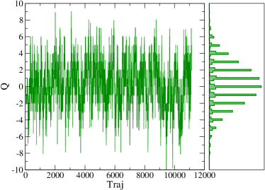
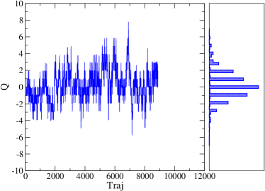
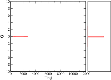
Figure 1: Check for the correct sampling of the topological charge. (Upper left) Topological charge time history and histogram for $a=0.0824\,\mathrm{fm}$ on a $32^{4}$ lattice. (Upper right) Topological charge time history and histogram for $a=0.0572\,\mathrm{fm}$ on a $48^{4}$ lattice. (Lower) Topological charge time history for $a=0.0397\,\mathrm{fm}$ on a $40^{4}$ lattice; in this case the run was stopped earlier because of the visible freezing of the topological charge. Note that the upper histories correspond to approximately the same physical volume: hence the visible shrink in the topological charge distribution is the actual effect of the approach to the continuum limit (see the discussion in Sec. 3).

3 Numerical Results

The main purpose of our numerical study is to provide results for the $\theta$-dependence of QCD at finite temperature, in particular above the pseudo-critical temperature, in order to take them as an input for axion phenomenology. However, in order to make sure that our lattice discretization is accurate enough to reproduce the chiral properties of light fermions, we have also performed numerical simulations at zero or low temperature, where results can be compared to reliable analytic predictions.

Indeed, at zero temperature, the full $\theta$ dependence of the QCD partition function, can be estimated reliably using chiral Lagrangians Weinberg:1977ma ; DiVecchia:1980ve ; Leutwyler:1992yt . In particular, at leading order in the expansion, $\chi$ and $b_{2}$ can be written just in terms of $m_{\pi}$, $f_{\pi}$ and $z=m_{u}/m_{d}$ as

$$\chi^{\rm LO}=\frac{z}{(1+z)^{2}}m_{\pi}^{2}f_{\pi}^{2}\,,\qquad b_{2}^{\rm LO}=-\frac{1}{12}\frac{1+z^{3}}{(1+z)^{3}}\,.$$ (15)

NLO corrections have been computed in Mao:2009sy ; Guo:2015oxa ; diCortona:2015ldu and are of the order of percent for physical values of the light quark masses. Using the estimate in diCortona:2015ldu we have $\chi^{1/4}=75.5(5)$ MeV and $b_{2}=-0.029(2)$ for $z=0.48(3)$, while $\chi^{1/4}=77.8(4)$ MeV and $b_{2}=-0.022(1)$ for $z=1$ used here. Note that for pure SU(3) Yang-Mills these numbers become $\chi^{1/4}_{N_{f}=0}\approx 180$ MeV Alles:1996nm ; DelDebbio:2002xa ; DelDebbio:2004ns ; Durr:2006ky ; Luscher:2010ik ; Cichy:2015jra ; Ce:2015qha and $b_{2,N_{f}=0}=-0.0216(15)$ Bonati:2015sqt (see also Refs. DelDebbio:2002xa ; D'Elia:2003gr ; Giusti:2007tu ; Panagopoulos:2011rb ; Ce:2015qha for previous determinations in the literature).

ChPT provides a prediction at finite temperature as well. In particular we have

$$\chi_{\rm ChPT}(T) =\chi(0)\,\left(1-\frac{3}{2}\frac{T^{2}}{f_{\pi}^{2}}\,J_{1}\left[\frac{T^{2}}{m_{\pi}^{2}}\right]\right)\,,$$ (16)

$$b_{2}^{\rm ChPT}(T) =b_{2}(0)\,\left(1+\frac{9}{2}\frac{m_{\pi}^{2}}{f_{\pi}^{2}}\,\frac{z(1+z)}{1+z^{3}}J_{2}\left[\frac{T^{2}}{m_{\pi}^{2}}\right]\right)\,,$$

where the functions $J_{n}$ are defined in Ref. diCortona:2015ldu . However, at temperatures around and above $T_{c}$, the chiral condensate drops and chiral Lagrangians break down, so that the finite $T$ predictions in Eq. (16) are expected to fail. In this regime non-perturbative computations based on first principle QCD are mandatory.

3.1 Zero Temperature

In Tab. 2 we report our determinations of the topological susceptibility on $N_{s}^{4}$ lattices for several values of $N_{s}$ and different lattice spacings. The results on the three smallest lattice spacings are also plotted in Fig. 2.

In order to extract the infinite volume limit of $\chi$ at fixed lattice spacing, one can either consider only results obtained on the largest available lattices and fit them to a constant, or try to model the behavior of $\chi$ with the lattice size using all available data. We have followed both procedures in order to better estimate possible systematics.

The topological susceptibility can be written as the integral of the two point function of the topological charge density; since the $\eta^{\prime}$ is the lightest intermediate state that significantly contributes to this two point function (three pions states are OZI suppressed), one expects the leading asymptotic behavior to be

$$\chi_{N_{s}}\sim\chi_{\infty}+Ce^{-aN_{s}m_{\eta^{\prime}}}\ ,$$ (17)

where $C$ is an unknown constant. This form nicely fits data in the whole available range of $aN_{s}$ (see Fig. 2), both when $m_{\eta^{\prime}}$ is fixed to its physical value and when it is left as a fit parameter. The results obtained using this last procedure (which gives the most conservative estimates) are reported in Tab. 2 and correspond to the entries denoted by $N_{s}=\infty$. On the other hand, a fit to a constant value works well when using only data coming from lattices with $aN_{s}>1.5\,\mathrm{fm}$, and provides consistent results within errors. This analysis makes also us confident that results obtained on the lattices with $a\simeq 0.1249$ fm and $a\simeq 0.0989$ fm, where a single spatial volume is available with $aN_{s}>3$ fm, are not affected by significant finite size effects.

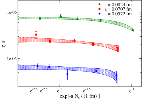
Figure 2: Volume dependence of the topological susceptibility for different lattice spacings. The lattice extent is reported in physical units, while $\chi$ in lattice spacing units. Bands represent best fits to Eq. (17) for the infinite volume limit extrapolation.

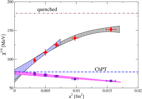
Figure 3: Continuum limit of the topological susceptibility: our final result is $\chi^{1/4}=73(9)\,\mathrm{MeV}$. Also shown is the value expected from chiral perturbation theory, denoted by the horizontal dashed line, together with the quenched value. Square points correspond to the combination $\chi^{1/4}_{tc}(a)$ defined in Eq. (20).

In Fig. 3 we plot $\chi^{1/4}$, extrapolated to infinite volume, against the square of the lattice spacing, together with the ChPT prediction. Finite cut-off effects are significant, especially for $a\gtrsim 0.1\,\mathrm{fm}$, meaning that we are not close enough to the continuum limit to reproduce the correct chiral properties of light quarks. In the case of staggered quarks, such lattice artifacts originate mostly from the fact that the full chiral symmetry group is reproduced only in the continuum limit, so that the pion spectrum is composed of a light pseudo-Goldstone boson and other massive states which become degenerate only as $a\to 0$. The physical signal vanishes in the chiral limit whereas this is not the case for its discretization effects. This means that it is necessary to work on very fine lattice spacings in order to keep these effects under control, a task which is particularly challenging with present algorithms, because of the freezing of the topological charge.

Despite the large cut-off effects, we can perform the continuum extrapolation of our data. If one considers only the three finest lattice spacings, the finite cut-off effects for this quantity can be parametrized as simple $O(a^{2})$ corrections

$$\chi^{1/4}(a)=\chi^{1/4}+Ba^{2}$$ (18)

and a best fit yields $\chi^{1/4}=73(9)$ MeV, while in order to describe the whole range of available data one must take into account $O(a^{4})$ corrections as well, i.e.

$$\chi^{1/4}(a)=\chi^{1/4}+Ba^{2}+Ca^{4}\,,$$ (19)

obtaining $\chi^{1/4}=69(9)$ MeV. Both best fits are reported in Fig. 3. Therefore we conclude that the continuum extrapolation is already under control with the available lattice data, and is in satisfactory agreement with the predictions of chiral perturbation theory.

In order to further inquire about the reliability of our continuum extrapolation and the importance of the partial breaking of chiral symmetry in the staggered discretization, we studied the combination

$$\chi^{1/4}_{tc}(a)=a\chi^{1/4}(a)\frac{m_{\pi}^{\mathrm{phys}}}{am_{ngb}(a)}\ .$$ (20)

Here $m_{ngb}(a)$ is the mass of one of the non-Goldstone pions, i.e. of a state that becomes massless in the chiral limit only if the continuum limit is performed; since in the continuum $m_{ngb}(a)\to m_{\pi}^{\mathrm{phys}}$, this ratio converges to $\chi^{1/4}$ as $a\to 0$. The state with taste structure $\gamma_{i}\gamma_{\mu}$ was used, whose mass is close to the root mean square value of all the taste states (see Ref. physline2 Fig. 2) and the values of $\chi^{1/4}_{tc}(a)$ are shown in Fig. 3 as square points. It is clear that the combination $\chi^{1/4}_{tc}(a)$ strongly reduces lattice artefacts with respect to $\chi^{1/4}(a)$, moreover a linear fit in $a^{2}$ well describes data for all available lattice spacings, giving the result $\chi^{1/4}=77(3)$. Although a complete study of the systematics affecting $\chi^{1/4}_{tc}(a)$ was not performed (e.g. the dependence of $m_{ngb}(a)$ on the lattice size was not studied, just the largest size was used), this is a strong indication that the dominant source of lattice artefacts in $\chi^{1/4}(a)$ is the chiral symmetry breaking present at finite lattice spacing in the staggered discretization.

$N_{s}$	$a$ [fm]	$\chi a^{4}$
32	0.1249	$8.55(32)\times 10^{-5}$
32	0.0989	$2.22(10)\times 10^{-5}$
12	0.0824	$4.14(20)\times 10^{-6}$
16	0.0824	$6.60(45)\times 10^{-6}$
20	0.0824	$7.17(36)\times 10^{-6}$
24	0.0824	$8.21(70)\times 10^{-6}$
32	0.0824	$7.32(39)\times 10^{-6}$
$\infty$	0.0824	$7.50(40)\times 10^{-6}$
16	0.0707	$1.57(16)\times 10^{-6}$
20	0.0707	$2.06(15)\times 10^{-6}$
24	0.0707	$2.42(16)\times 10^{-6}$
32	0.0707	$2.41(19)\times 10^{-6}$
40	0.0707	$3.29(56)\times 10^{-6}$
$\infty$	0.0707	$2.60(36)\times 10^{-6}$
20	0.0572	$4.34(90)\times 10^{-7}$
24	0.0572	$5.40(76)\times 10^{-7}$
32	0.0572	$4.7(1.2)\times 10^{-7}$
40	0.0572	$6.61(96)\times 10^{-7}$
48	0.0572	$6.88(87)\times 10^{-7}$
$\infty$	0.0572	$6.60(82)\times 10^{-7}$

Table 2: Topological susceptibility in lattice units, measured on several $N_{s}^{4}$ lattices for different values of the lattice spacing. Values denoted by $N_{s}=\infty$ correspond to the thermodynamical extrapolation and they are obtained by a fit to exponential without fixing $m_{\eta^{\prime}}$ to its physical value, see Eq. (17).

3.2 Finite Temperature

Finite temperature simulations can in principle be affected by lattice artifacts comparable to those present at $T=0$. For that reason, we have limited our finite $T$ simulations to the three smallest lattice spacings explored at $T=0$, i.e. those in the scaling window adopted for the extrapolation to the continuum limit with only $O(a^{2})$ corrections. At fixed lattice spacing the temperature has been varied by changing the temporal extent $N_{t}$ of the lattice and, in all cases, we have fixed $N_{s}=48$. This gives a spatial extent equal or larger than those explored at $T=0$ and an aspect ratio $N_{s}/N_{t}\geq 3$ for all explored values of $N_{t}$. The absence of significant finite volume effects has also been verified directly by comparing results with those obtained on $N_{t}\times 40^{3}$ lattices. In Tab. 3 we report the numerical values obtained for the topological susceptibility, for the ratio $\chi(T,a)/\chi(T=0,a)$ (where for $\chi(T=0,a)$ the infinite volume extrapolation has been taken) and for the cumulant ratio $b_{2}$.

$N_{t}$	$a$ [fm]	$T/T_{c}$	$\chi(T,a)a^{4}$	$\frac{\chi(T,a)}{\chi(0,a)}$	$b_{2}$
16	0.0824	0.964	$6.12(48)\cdot 10^{-6}$	$0.817(75)$	-0.23(33)
14	0.0824	1.102	$5.25(47)\cdot 10^{-6}$	$0.701(70)$	-0.191(95)
12	0.0824	1.285	$4.04(11)\cdot 10^{-6}$	$0.539(29)$	-0.003(25)
10	0.0824	1.542	$2.87(12)\cdot 10^{-6}$	$0.383(23)$	-0.083(29)
8	0.0824	1.928	$1.296(97)\cdot 10^{-6}$	$0.173(15)$	-0.065(25)
24	0.0707	0.749	$2.82(36)\cdot 10^{-6}$	$1.08(18)$	-0.11(12)
16	0.0707	1.124	$1.53(15)\cdot 10^{-6}$	$0.589(84)$	-0.057(43)
14	0.0707	1.284	$1.385(79)\cdot 10^{-6}$	$0.532(62)$	-0.019(30)
12	0.0707	1.498	$1.05(11)\cdot 10^{-6}$	$0.403(60)$	-0.101(21)
10	0.0707	1.798	$7.87(87)\cdot 10^{-7}$	$0.302(46)$	-0.096(26)
8	0.0707	2.247	$3.41(31)\cdot 10^{-7}$	$0.131(18)$	-0.077(18)
6	0.0707	2.996	$1.22(21)\cdot 10^{-7}$	$0.0469(94)$	-0.076(10)
16	0.0572	1.389	$2.92(41)\cdot 10^{-7}$	$0.41(16)$	-0.049(17)
14	0.0572	1.587	$2.04(32)\cdot 10^{-7}$	$0.29(11)$	-0.058(16)
12	0.0572	1.852	$1.43(19)\cdot 10^{-7}$	$0.202(79)$	-0.0626(90)
10	0.0572	2.222	$8.3(1.4)\cdot 10^{-8}$	$0.118(48)$	-0.0705(74)
8	0.0572	2.777	$4.85(86)\cdot 10^{-8}$	$0.068(27)$	-0.091(11)
6	0.0572	3.703	$2.51(72)\cdot 10^{-8}$	$0.035(16)$	-0.0792(12)

Table 3: Finite temperature results; in all cases $N_{s}=48$ was used.

$T_{cut}/T_{c}$	$A_{0}$ (MeV)	$A_{1}$(fm-2)	$A_{2}$
1.2	76.0(5.1)	103(17)	-0.671(40)
1.4	80.2(6.9)	100(20)	-0.728(57)
1.6	86(10)	85(24)	-0.750(80)
2.0	83(18)	97(53)	-0.718(14)

Table 4: Best fit values for the coefficients in (21) obtained by fitting only data corresponding to temperatures $T>T_{cut}$.

$T_{cut}/T_{c}$	$D_{0}$	$D_{1}$(fm-2)	$D_{2}$
1.2	1.17(24)	-2(28)	-2.71(15)
1.4	1.56(39)	-12(30)	-3.02(23)
1.6	1.81(76)	-33(32)	-2.99(39)
2.0	1.8(1.5)	2(22)$\times 10^{3}$	-2.90(65)

Table 5: Best fit values for the coefficients in (22) obtained by fitting only data corresponding to temperatures $T>T_{cut}$.

Results for $\chi^{1/4}$ as a function of $T/T_{c}$, where $T_{c}=155$ MeV, are reported in Fig. 4 for the three different lattice spacings. The dependence on $a$ is quite strong, as expected from the $T=0$ case. Inspired by the instanton gas prediction, Eq. (8), we have performed a fit with the following ansatz

$$\chi^{1/4}(a,T)=A_{0}(1+A_{1}a^{2})\left(\frac{T}{T_{c}}\right)^{A_{2}}\ ,$$ (21)

which also takes into account the dependence on $a$ and nicely describes all data in the range $T>1.2\,T_{c}$ with $\chi^{2}/\mathrm{dof}\simeq 0.7$. In Tab. 4 we report the best fit values obtained performing the fit in the region $T>T_{cut}$ for some $T_{cut}$ values; best fit curves are reported in Fig. 4 as well, together with a band corresponding to the continuum extrapolation.

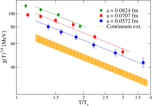
Figure 4: Continuum extrapolation of the fourth root topological susceptibility, using the function $\chi^{1/4}(a,T)=A_{0}(1+A_{1}a^{2})(T/T_{c})^{A_{2}}$. Only data corresponding to $T\gtrsim 1.2T_{c}$ have been used in the fit.

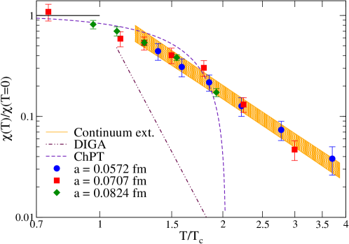
Figure 5: Ratio of the topological susceptibilities $\chi(T)/\chi(T=0)$, evaluated at fixed lattice spacing. The horizontal solid line describes trivial scaling $\chi(T)=\chi(T=0)$, while the dashed line is the prediction from finite temperature ChPT and the dashed-dotted line shows the slope predicted by DIGA computation. The band corresponds to the continuum extrapolation using the function $\chi(a,T)/\chi(a,T=0)=D_{0}(1+D_{1}a^{2})(T/T_{c})^{D_{2}}$, only data corresponding to $T\gtrsim 1.2T_{c}$ have been used in the fit.

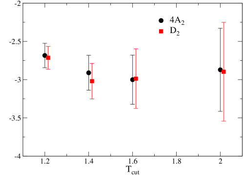
Figure 6: Plot of the exponent of the power-law behavior of $\chi(T)$, extracted from fit to Eqs. (21) and (22) for $T>T_{cut}$ (see Tabs. 4-5). The value predicted by the dilute instanton gas approximation and perturbation theory is $4A_{2},D_{2}\sim-8$.

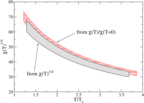
Figure 7: Comparison of the two continuum extrapolations for $\chi(T)^{1/4}$. Continuum extrapolated results for $\chi(T)/\chi(0)$ have been multiplied by the ChPT prediction for $\chi(0)$.

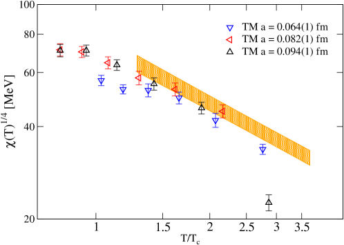
Figure 8: Comparison of our continuum extrapolated $\chi^{1/4}(T)$ (band) with results from Ref. Trunin:2015yda . Data for $\chi(T)$ obtained at unphysical quark masses have been rescaled according to the DIGA relation $\chi(T)\sim m_{q}^{2}\sim m_{\pi}^{4}$.

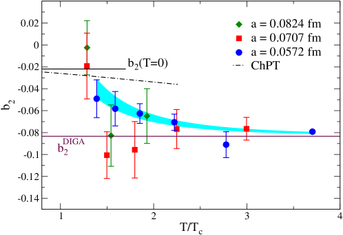
Figure 9: $b_{2}$ evaluated at three lattice spacing. The horizontal solid lines correspond to the value of $b_{2}$ at $T=0$ predicted by ChPT (which is about $-0.022$) and to the instanton-gas expected value $b_{2}^{DIGA}=-1/12$. The dotted-dashed line is the prediction of finite temperature ChPT, while the light blue band is the result of a fit to the smallest lattice spacing data using Eq. (26) with $d_{2}$ independent of $T$.

It is remarkable that most of the lattice artifacts disappear when one considers, in place of $\chi$ itself, the ratio $\chi(T,a)/\chi(T=0,a)$, whose dependence on the lattice spacing is indeed quite mild. That is clearly visible in Fig. 5. Also in this case we have adopted a fit ansatz similar to Eq. (21)

$$\frac{\chi(a,T)}{\chi(a,T=0)}=D_{0}(1+D_{1}a^{2})\left(\frac{T}{T_{c}}\right)^{D_{2}}\ ,$$ (22)

which well fits all data in the range $T>1.2\,T_{c}$ with a $\chi^{2}/\mathrm{dof}\simeq 1$. The best fit curves and the continuum extrapolation are shown in Fig. 5. The best fit parameters, again for different $T_{cut}$ values, are reported in Tab. 5. It is important to note, in order to assess the reliability of our continuum limit, that the two different extrapolations, Eqs. (21) and (22), provide perfectly consistent results: that can be appreciated both from Fig. 6, where we compare the two coefficients $D_{2}$ and $4A_{2}$, and from Fig. 7, where we directly compare the two continuum extrapolations. As a further check, we have also verified that by fitting $[\chi(a,T)/\chi(a,T=0)]^{1/4}$ we obtain results in perfect agreement with the ones obtained by fitting $\chi(a,T)/\chi(a,T=0)$. As an example, using in the fit the values corresponding to $T>1.2T_{c}$ one obtains for the exponent the value $-0.674(38)$, to be compared with $D_{2}/4$ from the first line of Tab. 5 and $A_{2}$ from the first line of Tab. 4. However in the following analysis we will refer to results obtained through the ratio $\chi(T)/\chi(0)$, which is the quantity showing smaller finite cut-off corrections.

Let us now comment on our results for the topological susceptibility. For temperatures below or around $T_{c}$, the temperature dependence is quite mild and, for temperatures up to $T\simeq 1.2\,T_{c}$, even compatible with the prediction from ChPT, which is reported in Fig. 5 for comparison. Then, for higher values of $T$, a sharp power law drop starts. However, it is remarkable that the power law exponent is smaller, by more than a factor two, with respect to the instanton gas computation, Eq. (8), which predicts $D_{2}\simeq-8$ in the case of three light flavors (the dependence on the number of flavor is however quite mild). DIGA is expected to provide the correct result in a region of asymptotically large temperatures, which however seems to be quite far from the range explored in the present study, which goes up to $T\simeq 4\,T_{c}$.

This is in sharp contrast with the quenched theory, where the DIGA power law behavior sets in at lower temperatures Borsanyi:2015cka ; Berkowitz:2015aua . In order to allow for a direct comparison, we have reported the DIGA prediction in Fig. 5, after fixing it by imposing $\chi(T_{c})=\chi(0)$ as an overall normalization. As we discuss in the following section, the much milder drop of $\chi$ as a function of $T$ has important consequences for axion cosmology.

A determination of the topological susceptibility has been presented in Ref. Buchoff:2013nra , based on the Domain Wall discretization, in the range $T/T_{c}\sim$ 0.9 - 1.2. Since the data have been produced with different lattice spacings at different temperatures, it is however difficult to compare their results with ours. An extended range of $T$ has been explored in Ref. Trunin:2015yda in the presence of twisted mass Wilson fermions, reporting a behavior similar to that observed in this study, although with larger values of the quark masses (corresponding to a pion mass $m_{\pi}\sim 370$ MeV). The comparison is performed in Fig. 8, and shows a reasonable agreement if results from Ref. Trunin:2015yda are rescaled according to the mass dependence expected from DIGA, i.e. $\chi(T)\sim m_{q}^{2}\sim m_{\pi}^{4}$.

Let us now turn to a discussion of our results for the coefficient $b_{2}$ (defined in Eq. (5)), which is related to the non-gaussianity of the topological charge distribution and gives information about the shape of the $\theta$-dependent part of the free energy density. Data for $b_{2}$ are reported in Fig. 9. For $T<T_{c}$ this observable is too noisy to give sensible results but a reasonable guess, motivated by what happens in the quenched case and by the ChPT prediction, is that $b_{2}$ is almost temperature independent for $T\lesssim T_{c}$, like the topological susceptibility. In the high temperature region $b_{2}$ can instead be measured with reasonable accuracy and, due to the peculiar dependence of the noise on this observable on $\chi{\cal V}$, data on the smaller lattice spacing turned out to be significantly more precise than the others (see the discussion in Ref. Bonati:2015sqt ). While data clearly approach the dilute instanton gas prediction $b_{2}^{DIGA}=-1/12$ at high temperature, deviations from this value are clearly visible on all the lattice spacings for $T\simeq 1.3~{}T_{c}$ and, for the smallest lattice spacing, also up to $T\sim 2.5~{}T_{c}$.

This is in striking contrast to what is observed in pure gauge theory, where deviations from $-1/12$ are practically absent for $T\gtrsim 1.15~{}T_{c}$, with a precision higher than $10\%$ Bonati:2013tt ; Borsanyi:2015cka ; Bonati:2015uga ; Xiong:2015dya . As discussed in the introduction deviations from $b_{2}^{DIGA}$ cannot be simply ascribed to a failure of perturbation theory (like e.g. for the behavior of $\chi(T)$) but are instead unambiguous indications of interaction between instantons. Another difference with respect to the quenched case is that in the pure gauge theory (with both gauge groups $SU(N)$ and $G_{2}$, see Bonati:2013tt ; Bonati:2015uga ) the asymptotic value is approached from below, while in the present case it is approached from above. These peculiar features can be related to a different interaction between instantons mediated by light quarks, as it is clear from the following discussion.

To describe deviations from the instanton gas behavior it is convenient to use the parametrization of $\mathcal{F}(\theta,T)$ introduced in Ref. Bonati:2013tt :

$$\mathcal{F}(\theta,T)=\sum_{n>0}c_{2(n-1)}(T)\sin^{2n}(\theta/2)\ .$$ (23)

Indeed it is not difficult to show that every even function of $\theta$ of period $2\pi$ can be written in this form, and the main advantage of this form is that the value of coefficient $c_{2n}$ influences only $b_{2j}$ with $j\geq n$: in particular

$$\chi(T)=c_{0}(T)/2;\quad b_{2}(T)=-\frac{1}{12}+\frac{c_{2}(T)}{8\chi(T)};$$ (24)

$$b_{4}(T)=\frac{1}{360}-\frac{c_{2}(T)}{48\chi(T)}+\frac{c_{4}(T)}{32\chi(T)}\ .$$

Since the coefficients $c_{2n}$ parametrize deviations from the instanton gas that manifest themselves only in higher-cumulants of the topological charge, it is natural to interpret Eq. (23) as a virial expansion, in which the role of the “density” is played by the first coefficient (i.e. the topological susceptibility $\chi$), and to introduce the dimensionless coefficients $d_{2n}$ by

$$c_{2(n-1)}(T)=d_{2(n-1)}(T)\frac{\chi(T)^{n}}{\chi(T=0)^{n-1}}\ ,$$ (25)

where $\chi(T=0)$ was used just as a dimensional normalization and one expects a mild dependence of $d_{2(n-1)}(T)$ on the temperature, since the strongly dependent component $\chi(T)^{n}$ have been factorized. To lowest order we thus have

$$b_{2}(T)=-\frac{1}{12}+\frac{d_{2}}{8}\frac{\chi(T)}{\chi(T=0)}\ ,$$ (26)

which nicely describes the $b_{2}$ data for the smallest lattice spacing using $d_{2}=0.80(16)$, see Fig. 9, where the expression $\chi(T)/\chi(T=0)\simeq(T_{c}/T)^{2.7}$ was used.

In the spirit of a virial expansion interpretation of Eq. (23), the coefficient $d_{2}$ can be considered as the lowest order interaction term between instantons. In particular, a positive value of $d_{2}$ corresponds to an attractive potential, which is in sharp contrast with the pure gauge case, where a repulsive, negative value of $d_{2}$ is observed. This peculiar difference can be surely interpreted in terms of effective instanton interactions mediated by light quarks, which are likely also responsible for the much slower convergence, with respect to the quenched case, to the DIGA prediction.

4 Implications for Axion Phenomenology

The big departure of the results for the topological susceptibility at finite temperature from the DIGA prediction has a strong impact on the computation of the axion relic abundance. In particular the model independent contribution from the misalignment mechanism is determined to be diCortona:2015ldu

$$\Omega_{a}^{mis}=\frac{86}{33}\frac{\Omega_{\gamma}}{T_{\gamma}}\frac{n_{a}^{\star}}{s^{\star}}m_{a}\,,$$ (27)

where $\Omega_{\gamma}$ and $T_{\gamma}$ are the present abundance and temperature of photons while $n_{a}^{\star}/s^{\star}$ is the ratio between the comoving number density $n_{a}=\langle m_{a}a^{2}\rangle$ and the entropy density $s$ computed at a late time $t_{\star}$ such that the ratio $n_{a}/s$ became constant. The number density $n_{a}$ can be extracted by solving the axion equation of motion

$$\ddot{a}+3H\dot{a}+V^{\prime}(a)=0\,,$$ (28)

The temperature (and time) dependence of the Hubble parameter $H$ is determined by the Friedmann equations and the QCD equation of state. The biggest uncertainties come therefore from the temperature dependence of the axion potential $V(a)$. At high temperatures the Hubble friction dominates over the vanishing potential and the field is frozen to its initial value $a_{0}$. As the Universe cools the pull from the potential starts winning over the friction (this happens when $T\approx T_{osc}$, defined as $m_{a}(T_{osc})\approx 3H(T_{osc})$) and the axion starts oscillating around the minimum. Shortly after $H$ becomes negligible and the mass term is the leading scale in Eq. (28). In this regime the approximate WKB solution has the form

$$a(t) \sim A(t)\cos\left(\int_{t_{0}}^{t}dt^{\prime}m_{a}(t^{\prime})\right)=$$ (29)

$$=a(t_{0})\,\left(\frac{m_{a}(t_{0})R^{3}(t_{0})}{m_{a}(t)R^{3}(t)}\right)^{1/2}\,\cos\left(\int_{t_{0}}^{t}dt^{\prime}m_{a}(t^{\prime})\right)\,,$$

where $R(t)$ is the cosmic scale factor. Since the energy density is given by $\rho_{a}\sim m_{a}^{2}A^{2}/2$, the solution (29) implies that what is conserved in the comoving volume is not the energy density but $N_{a}=\rho_{a}R^{3}/m_{a}$, which can be interpreted as the number of axions Preskill:1982cy ; Abbott:1982af ; Dine:1982ah . Through the conservation of the comoving entropy $S$, it follows that $n_{a}^{\star}/s^{\star}$ becomes an adiabatic invariant. Hence, it is enough to integrate the equation of motion (28) in the small window around the time when $T\approx T_{osc}$. We integrated numerically Eq. (28) in the interval between the time when $m_{a}=H/10$ to that corresponding to $m_{a}=2400H$ and extract the ratio $n_{a}^{\star}/s^{\star}$ when $m_{a}\sim 300H$, namely a factor a hundred since the oscillation regime begins. The value for $T_{osc}$ varies from $T_{c}$ to several GeV depending on the axion decay parameter $f_{a}$ and the temperature dependence of the axion potential. More details about this standard computation can be found for example in Wantz:2009it ; diCortona:2015ldu . In order to estimate the uncertainty in the results given below we varied the fitting parameters of the topological susceptibility $D_{2}$, $D_{0}$ and those relative to the QCD equation of state physline2 within the quoted statistical and systematic errors.

Given that $b_{2}(T)$ converges relatively fast to the value predicted by a single cosine potential, we can assume $V(a)=-\chi(T)\cos(a/f_{a})$ for $T\gtrsim T_{c}$. Using the most conservative results for the fit of $\chi(T)$, i.e. $\chi(T)/\chi(0)=(1.8\pm 1.5)(T_{c}/T)^{2.90\pm 0.65}$, in Fig. 10 we plot the prediction for the parameter $f_{a}$ as a function of the initial value of the axion field $\theta_{0}=a_{0}/f_{a}$ assuming that the misalignment axion contribution make up for the whole observed dark matter abundance, $\Omega_{\rm DM}=0.259(4)$ Ade:2015xua . We also plot the case where the axion misalignment contribution accounts only for part (10% for definiteness) of the dark matter abundance.

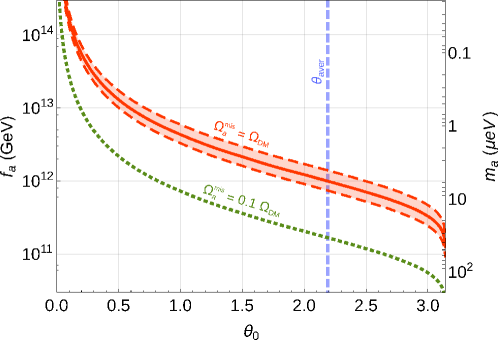
Figure 10: Values of the axion decay constant $f_{a}$ as a function of the initial field value $\theta_{0}=a_{0}/f_{a}$ such that the axion misalignment contribution matches the full or a tenth of the observed dark matter abundance (red band or dotted green line respectively). When the PQ symmetry is broken only after inflation the axion abundance is reproduced by choosing $\theta_{0}\approx 2.2$, i.e. the vertical blue dashed line.

In some cases the axion field acquires all possible values within the visible horizon, therefore the initial condition to the Eq. (28) needs to be integrated over. This happens if the PQ symmetry is broken only after inflation or if the PQ symmetric phase is temporarily restored after inflation (e.g. if the Hubble scale during inflation or the maximum temperature at reheating are at or above the PQ scale $f_{a}$). Numerically it corresponds to choosing $\theta_{0}\approx 2.2$ and the value of the PQ scale in this case is fixed to:

$$f_{a}(\theta_{0})=(1.00^{+0.40}_{-0.26}{}^{+0.07}_{-0.18}\pm 0.06)\cdot 10^{12}~{}{\rm GeV}\,,$$ (30)

where the errors correspond respectively to the uncertainties on the fit parameters $D_{2}$, $D_{0}$, and to the error in the QCD equation of state. Note that, in this case, also other contributions from topological defects are expected to contribute. In case their effects are not negligible, or if axions are not responsible for the whole dark matter abundance, the value above should just be read as an upper bound to the PQ scale.

The value in Eq. (30) is almost one order of magnitude bigger than the one computed with instantons techniques ($f_{a}\lesssim 0.2\cdot 10^{12}$ GeV), which in fact corresponds to the value we instead get for one tenth of the dark matter abundance.

Some few remarks are in order. While the uncertainties on the axion mass fit we used are not small, the final axion abundance is rather insensitive to them and the prediction for $f_{a}$ has therefore a good precision. The results above, however, rely on the extrapolation of the axion mass fit formula up to few GeV, where no lattice data is available. In particular for the value of $f_{a}$ in Eq. (30) the axion field starts oscillating around $T_{osc}=4.3$ GeV. An even longer extrapolation is required for $f_{a}=1.67\cdot 10^{11}$ GeV, corresponding to $\Omega_{a}^{\rm mis}=0.1\,\Omega_{\rm DM}$, where the axion starts oscillating around $T_{osc}=7.2$ GeV.

Given the stability of the fit in the accessible window of temperatures (see Fig. 6) big changes in the axion mass behavior are not expected. Still, extending the analysis to even higher temperatures would be extremely useful to control better the extrapolation systematics.

Larger values of $f_{a}$ corresponds instead to smaller $T_{osc}$, for example for $f_{a}=10^{13}$ GeV, $T_{osc}=2.2$ GeV while for $f_{a}=10^{14}$ GeV, $T_{osc}=1.1$ GeV. Above these values no extrapolation is required and the corresponding results are free from the extrapolation uncertainties.

5 Conclusions

We studied the topological properties and the $\theta$-dependence for $N_{f}=2+1$ QCD along a line of constant physics, corresponding to physical quarks masses, and for temperatures up to $4\,T_{c}$, where $T_{c}=155$ MeV is the pseudo-critical temperature at which chiral symmetry restoration takes place. We explored several lattice spacings, in a range $0.05-0.12$ fm, in order to perform a continuum extrapolation of our results. Our investigation at even smaller lattice spacings has been hindered by a severe slowing down in the decorrelation of the topological charge.

At zero temperature we observe large cut-off effects for the topological susceptibility. Nevertheless we are able to perform a continuum extrapolation, obtaining from the three finest lattice spacings $\chi^{1/4}=73(9)$ MeV, in reasonable agreement with the ChPT prediction in the case of degenerate light flavors, $\chi^{1/4}_{\rm ChPT}=77.8(4)$ MeV.

At finite temperature we observe that cut-off effects are drastically reduced when one considers the ratio $\chi(T)/\chi(T=0)$, which turns out to be the most convenient quantity to perform a continuum extrapolation. The agreement with ChPT persists up to around $T_{c}$. At higher temperatures the topological susceptibility presents the power-law dependence $\chi(T)/\chi(0)=D_{0}(T/T_{c})^{D_{2}}$, with $D_{2}\sim-3$. The exponent of the power-law behavior is however substantially smaller than the DIGA prediction, $D_{2}\sim-8$.

Regarding the shape of the $\theta$-dependent part of the free energy density, and in particular the lowest order coefficient $b_{2}$, a visible convergence to the instanton gas prediction is observed in the explored range. With respect to the pure gauge case, the convergence of $b_{2}$ to DIGA is slower and the deviation is opposite in sign  Bonati:2013tt ; Bonati:2015uga . This suggests a different interaction between instantons right above $T_{c}$, namely repulsive in the quenched case and attractive in full QCD Callan:1977gz .

The deviations from the dilute instanton gas predictions that we found in the present study have a significant impact on axions, resulting in particular in a shift of the axion dark matter window by almost one order of magnitude with respect to estimates based on DIGA. The softer temperature dependence of the topological susceptibility also changes the onset of the axion oscillations, which would now start at a higher temperatures ($T\sim 4$ GeV).

An important point is that this seems an effect directly related to the presence of light fermionic degrees of freedom: indeed, pure gauge computations Borsanyi:2015cka ; Berkowitz:2015aua observe a power-law behavior in good agreement with DIGA in a range of temperatures comparable to those explored in the present study.

One might wonder whether a different power law behavior might set in at temperatures higher than 1 GeV. That claims for future studies extending the range explored by us. The main obstruction to this extension is represented by the freezing of the topological modes at smaller lattice spacings which would be necessary to investigate such temperatures ($a<0.05$ fm). Such an obstruction could be overcome by the development of new Monte-Carlo algorithms. Proposals in this respect have been made in the past deForcrand:1997fm ; openbc and some new strategies have been put forward quite recently surfing ; endres . In view of the exploration of higher temperatures, one should also consider the inclusion of dynamical charm quarks.

- (1) R. D. Peccei and H. R. Quinn, Phys. Rev. Lett. 38, 1440 (1977).
- (2) R. D. Peccei and H. R. Quinn, Phys. Rev. D 16, 1791 (1977).
- (3) F. Wilczek, Phys. Rev. Lett. 40 (1978) 279.
- (4) S. Weinberg, Phys. Rev. Lett. 40 (1978) 223.
- (5) J. Preskill, M. B. Wise and F. Wilczek, Phys. Lett. B 120 (1983) 127.
- (6) L. F. Abbott and P. Sikivie, Phys. Lett. B 120 (1983) 133.
- (7) M. Dine and W. Fischler, Phys. Lett. B 120 (1983) 137.
- (8) E. Vicari and H. Panagopoulos, Phys. Rept. 470, 93 (2009) [arXiv:0803.1593 [hep-th]].
- (9) D. J. Gross, R. D. Pisarski and L. G. Yaffe, Rev. Mod. Phys. 53, 43 (1981).
- (10) T. Schäfer and E. V. Shuryak, Rev. Mod. Phys. 70, 323 (1998) [hep-ph/9610451].
- (11) T. R. Morris, D. A. Ross and C. T. Sachrajda, Nucl. Phys. B 255, 115 (1985).
- (12) A. Ringwald and F. Schrempp, Phys. Lett. B 459, 249 (1999) [hep-lat/9903039].
- (13) S. Borsanyi et al., Phys. Lett. B 752, 175 (2016) [arXiv:1508.06917 [hep-lat]].
- (14) C. Bonati, M. D’Elia, H. Panagopoulos and E. Vicari, Phys. Rev. Lett. 110, 252003 (2013) [arXiv:1301.7640 [hep-lat]].
- (15) C. Bonati, JHEP 1503, 006 (2015) [arXiv:1501.01172 [hep-lat]].
- (16) G. Y. Xiong, J. B. Zhang, Y. Chen, C. Liu, Y. B. Liu and J. P. Ma, Phys. Lett. B 752, 34 (2016) [arXiv:1508.07704 [hep-lat]].
- (17) B. Alles, M. D’Elia and A. Di Giacomo, Nucl. Phys. B 494, 281 (1997) [Erratum Nucl. Phys. B 679, 397 (2004)] [hep-lat/9605013].
- (18) B. Alles, M. D’Elia and A. Di Giacomo, Phys. Lett. B 483, 139 (2000) [hep-lat/0004020].
- (19) C. Gattringer, R. Hoffmann and S. Schaefer, Phys. Lett. B 535, 358 (2002) [hep-lat/0203013].
- (20) B. Lucini, M. Teper and U. Wenger, Nucl. Phys. B 715, 461 (2005) [hep-lat/0401028].
- (21) L. Del Debbio, H. Panagopoulos and E. Vicari, JHEP 0409, 028 (2004) [hep-th/0407068].
- (22) E. Berkowitz, M. I. Buchoff and E. Rinaldi, Phys. Rev. D 92, 034507 (2015) [arXiv:1505.07455 [hep-ph]].
- (23) A. Bazavov et al. [MILC Collaboration], Phys. Rev. D 81, 114501 (2010) [arXiv:1003.5695 [hep-lat]].
- (24) A. Bazavov et al. [MILC Collaboration], Phys. Rev. D 87, 054505 (2013) [arXiv:1212.4768 [hep-lat]].
- (25) K. Cichy et al. [ETM Collaboration], JHEP 1402, 119 (2014) [arXiv:1312.5161 [hep-lat]].
- (26) M. Bruno, S. Schaefer and R. Sommer [ALPHA Collaboration], JHEP 1408, 150 (2014) [arXiv:1406.5363 [hep-lat]].
- (27) H. Fukaya et al. [JLQCD Collaboration], PoS LATTICE 2014, 323 (2014) [arXiv:1411.1473 [hep-lat]].
- (28) B. Alles, G. Boyd, M. D’Elia, A. Di Giacomo and E. Vicari, Phys. Lett. B 389, 107 (1996) [hep-lat/9607049].
- (29) L. Del Debbio, H. Panagopoulos and E. Vicari, JHEP 0208, 044 (2002) [hep-th/0204125].
- (30) L. Del Debbio, G. M. Manca and E. Vicari, Phys. Lett. B 594, 315 (2004) [hep-lat/0403001].
- (31) S. Schaefer et al. [ALPHA Collaboration], Nucl. Phys. B 845, 93 (2011) [arXiv:1009.5228 [hep-lat]].
- (32) R. Kitano and N. Yamada, JHEP 1510, 136 (2015) [arXiv:1506.00370 [hep-ph]].
- (33) P. Weisz, Nucl. Phys. B 212, 1 (1983).
- (34) G. Curci, P. Menotti and G. Paffuti, Phys. Lett. B 130, 205 (1983) [Erratum-ibid. B 135, 516 (1984)].
- (35) C. Morningstar and M. J. Peardon, Phys. Rev. D 69, 054501 (2004) [hep-lat/0311018].
- (36) Y. Aoki, S. Borsanyi, S. Durr, Z. Fodor, S. D. Katz, S. Krieg and K. K. Szabo, JHEP 0906, 088 (2009) [arXiv:0903.4155 [hep-lat]].
- (37) S. Borsanyi, G. Endrodi, Z. Fodor, A. Jakovac, S. D. Katz, S. Krieg, C. Ratti and K. K. Szabo, JHEP 1011, 077 (2010) [arXiv:1007.2580 [hep-lat]];
- (38) S. Borsanyi, Z. Fodor, C. Hoelbling, S. D. Katz, S. Krieg and K. K. Szabo, Phys. Lett. B 730, 99 (2014) [arXiv:1309.5258 [hep-lat]].
- (39) H. Neuberger, Phys. Lett. B 417, 141 (1998) [hep-lat/9707022].
- (40) P. Hasenfratz, V. Laliena and F. Niedermayer, Phys. Lett. B 427, 125 (1998) [hep-lat/9801021].
- (41) M. Luscher, Phys. Lett. B 428, 342 (1998) [hep-lat/9802011].
- (42) M. Luscher, Phys. Lett. B 593, 296 (2004) [hep-th/0404034].
- (43) L. Giusti and M. Luscher, JHEP 0903, 013 (2009) [arXiv:0812.3638 [hep-lat]].
- (44) B. Berg, Phys. Lett. B 104, 475 (1981); Y. Iwasaki and T. Yoshie, Phys. Lett. B 131, 159 (1983); S. Itoh, Y. Iwasaki and T. Yoshie, Phys. Lett. B 147, 141 (1984); M. Teper, Phys. Lett. B 162, 357 (1985); E. -M. Ilgenfritz et al., Nucl. Phys. B 268, 693 (1986).
- (45) M. Luscher, Commun. Math. Phys. 293, 899 (2010) [arXiv:0907.5491 [hep-lat]].
- (46) M. Luscher, JHEP 1008, 071 (2010) [JHEP 1403, 092 (2014)] [arXiv:1006.4518 [hep-lat]].
- (47) C. Bonati and M. D’Elia, Phys. Rev. D 89, 105005 (2014) [arXiv:1401.2441 [hep-lat]].
- (48) K. Cichy, A. Dromard, E. Garcia-Ramos, K. Ottnad, C. Urbach, M. Wagner, U. Wenger and F. Zimmermann, PoS LATTICE 2014, 075 (2014) [arXiv:1411.1205 [hep-lat]].
- (49) Y. Namekawa, PoS LATTICE 2014, 344 (2015) [arXiv:1501.06295 [hep-lat]].
- (50) C. Alexandrou, A. Athenodorou and K. Jansen, Phys. Rev. D 92, 125014 (2015) [arXiv:1509.04259 [hep-lat]].
- (51) R. Sommer, PoS LATTICE 2013, 015 (2014) [arXiv:1401.3270 [hep-lat]].
- (52) Z. Fodor, K. Holland, J. Kuti, S. Mondal, D. Nogradi and C. H. Wong, JHEP 1409, 018 (2014) [arXiv:1406.0827 [hep-lat]].
- (53) P. Di Vecchia, K. Fabricius, G. C. Rossi and G. Veneziano, Nucl. Phys. B 192, 392 (1981).
- (54) C. Bonati, M. D’Elia and A. Scapellato, Phys. Rev. D 93, 025028 (2016) [arXiv:1512.01544 [hep-lat]].
- (55) P. Di Vecchia and G. Veneziano, Nucl. Phys. B 171 (1980) 253.
- (56) H. Leutwyler and A. V. Smilga, Phys. Rev. D 46, 5607 (1992).
- (57) Y. Y. Mao et al. [TWQCD Collaboration], Phys. Rev. D 80 (2009) 034502 [arXiv:0903.2146 [hep-lat]].
- (58) F. K. Guo and U. G. Meißner, Phys. Lett. B 749 (2015) 278 [arXiv:1506.05487 [hep-ph]].
- (59) G. G. di Cortona, E. Hardy, J. P. Vega and G. Villadoro, JHEP 1601, 034 (2016) [arXiv:1511.02867 [hep-ph]].
- (60) L. Del Debbio, L. Giusti and C. Pica, Phys. Rev. Lett. 94, 032003 (2005) [hep-th/0407052].
- (61) S. Durr, Z. Fodor, C. Hoelbling and T. Kurth, JHEP 0704, 055 (2007) [hep-lat/0612021].
- (62) M. Luscher and F. Palombi, JHEP 1009, 110 (2010) [arXiv:1008.0732 [hep-lat]].
- (63) K. Cichy et al. [ETM Collaboration], JHEP 1509, 020 (2015) [arXiv:1504.07954 [hep-lat]].
- (64) M. Cé, C. Consonni, G. P. Engel and L. Giusti, Phys. Rev. D 92, 074502 (2015) [arXiv:1506.06052 [hep-lat]].
- (65) M. D’Elia, Nucl. Phys. B 661, 139 (2003) [hep-lat/0302007].
- (66) L. Giusti, S. Petrarca and B. Taglienti, Phys. Rev. D 76, 094510 (2007) [arXiv:0705.2352 [hep-th]].
- (67) H. Panagopoulos and E. Vicari, JHEP 1111, 119 (2011) [arXiv:1109.6815 [hep-lat]].
- (68) M. I. Buchoff et al., Phys. Rev. D 89, 054514 (2014) [arXiv:1309.4149 [hep-lat]].
- (69) A. Trunin, F. Burger, E.-M. Ilgenfritz, M. P. Lombardo and M. Müller-Preussker, arXiv:1510.02265 [hep-lat].
- (70) O. Wantz and E. P. S. Shellard, Phys. Rev. D 82 (2010) 123508 [arXiv:0910.1066 [astro-ph.CO]].
- (71) P. A. R. Ade et al. [Planck Collaboration], arXiv:1502.01589 [astro-ph.CO].
- (72) C. G. Callan, Jr., R. F. Dashen and D. J. Gross, Phys. Rev. D 17, 2717 (1978).
- (73) P. de Forcrand, J. E. Hetrick, T. Takaishi and A. J. van der Sijs, Nucl. Phys. Proc. Suppl. 63, 679 (1998) [hep-lat/9709104].
- (74) M. Luscher and S. Schaefer, JHEP 1107, 036 (2011) [arXiv:1105.4749 [hep-lat]].
- (75) A. Laio, G. Martinelli and F. Sanfilippo, arXiv:1508.07270 [hep-lat].
- (76) M. G. Endres, R. C. Brower, W. Detmold, K. Orginos and A. V. Pochinsky, Phys. Rev. D 92, 114516 (2015) [arXiv:1510.04675 [hep-lat]].