Multipole decomposition of the nucleon transverse phase space

Abstract

We present a complete study of the leading-twist quark Wigner distributions in the nucleon, discussing both the $\mathsf{T}$-even and $\mathsf{T}$-odd sector, along with all the possible configurations of the quark and nucleon polarizations. We identify the basic multipole structures associated with each distribution in the transverse phase space, providing a transparent interpretation of the spin-spin and spin-orbit correlations of quarks and nucleon encoded in these functions. Projecting the multipole parametrization of the Wigner functions onto the transverse-position and the transverse-momentum spaces, we find a natural link with the corresponding multipole parametrizations for the generalized parton distributions and transverse-momentum dependent parton distributions, respectively. Finally, we show results for all the distributions in the transverse phase space, introducing a representation that allows one to visualize simultaneously the multipole structures in both the transverse-position and transverse-momentum spaces.

I Introduction

The concept of phase-space distributions borrowed from Classical Mechanics has been transposed to Quantum Mechanics Wigner:1932eb , where it finds numerous applications Balazs:1983hk ; Hillery:1983ms ; Lee:1995 . Phase-space distributions have also been defined in the context of Relativistic Field Theory Carruthers:1982fa ; Hakim:1976bn ; DeGroot:1980dk and more specifically in Quantum ChromoDynamics Elze:1986qd ; Ochs:1998qj ; Heinz:1983nx ; Heinz:1984yq ; Elze:1986hq . The six-dimensional version of these phase-space distributions has been discussed for the first time in connection with Generalized Parton Distributions (GPDs) in Refs. Ji:2003ak ; Belitsky:2003nz . However, in this case the physical interpretation is plagued by relativistic corrections. This issue has been solved in the light-front formalism by integrating over the longitudinal spatial dimension Soper:1976jc ; Burkardt:2000za ; Burkardt:2002hr ; Burkardt:2005hp , leading to five-dimensional phase-space distributions Lorce:2011kd which are related via a proper Fourier transform to Generalized Transverse-Momentum dependent Distributions (GTMDs) Meissner:2009ww ; Lorce:2011dv ; Lorce:2013pza .

The GTMDs recently received increasing attention due to the fact that they can be considered as the mother distributions of GPDs and Transverse-Momentum dependent Distributions (TMDs) Meissner:2009ww ; Lorce:2011dv ; Lorce:2013pza . Moreover, it turned out that they are naturally related to the parton orbital angular momentum (OAM) Lorce:2011kd ; Hatta:2011ku ; Lorce:2011ni ; Liu:2015xha . Except possibly at low-$x$ Martin:1999wb ; Khoze:2000cy ; Martin:2001ms ; Albrow:2008pn ; Martin:2009ku , no experimental process directly sensitive to GTMDs has been identified so far. Nevertheless, these distributions can be studied using phenomenological or perturbative models Meissner:2009ww ; Lorce:2011kd ; Kanazawa:2014nha ; Mukherjee:2014nya ; Liu:2014vwa ; Liu:2015eqa ; Miller:2014vla ; Mukherjee:2015aja ; Burkardt:2015qoa , and can also in principle be computed on a lattice Ji:2013dva .

In total, there are at leading twist 32 quark phase-space distributions among which half originate from naive $\mathsf{T}$-odd GTMDs. In a former work Lorce:2011kd , we studied the four naive $\mathsf{T}$-even distributions associated with longitudinal polarization. Here, we present for the first time a complete study of all the 32 distributions.

Even though the number of independent functions is fixed by hermiticity and space-time symmetries, the parametrization of the correlator is not unique. In some sense, choosing a particular parametrization amounts to choosing a particular basis for decomposing the correlator. One can change the basis, but not the number of independent basis elements. The choice of a particular decomposition is arbitrary and is often motivated by the simplicity of the mathematical expressions. However, simple mathematical expressions often turn out to have rather obscure physical interpretation.

In this work, we choose natural combinations of GTMDs corresponding to distributions for all the possible configurations of the target and quark polarizations, and perform a multipole decomposition of each of these distributions in the transverse phase space. This multipole analysis allows us to identify in a clear way all the possible spin-spin and spin-orbit correlations of quarks and nucleon in phase space, and has a direct connection with the spin densities in impact-parameter space described by GPDs and the transverse-momentum densities described by TMDs.

The plan of the manuscript is as follows. In Sec. II we review the definition of the Wigner distributions obtained by Fourier transform of the GTMDs to the impact-parameter space, and we summarize the transformation properties of these functions under time-reversal, parity and hermitian conjugation. In Sec. III, we outline the general method for the decomposition of the Wigner functions in basic multipoles in the transverse phase space, and we identify all the possible correlations between target polarization, quark polarization and quark OAM encoded in these phase-space distributions. In Sec. IV we introduce a new representation of the transverse phase space, which allows one to visualize the multipole structures simultaneously in both the transverse-momentum and transverse-position spaces. In Sec. V we present and discuss the results of both the $\mathsf{T}$-even and $\mathsf{T}$-odd distributions, for all the possible quark and target polarizations. Although the calculation is performed within a specific relativistic light-front constituent quark model Lorce:2011dv , we can draw general and model-independent conclusions about the physical information encoded in these functions. Finally, we summarize our results in Sec. VI.

II Polarized relativistic phase-space distributions

We introduce two lightlike four-vector $n_{\pm}$ satisfying $n_{+}\cdot n_{-}=1$. Any four-vector $a^{\mu}$ can then be decomposed as

$$a^{\mu}=a^{+}n^{\mu}_{+}+a^{-}n^{\mu}_{-}+a^{\mu}_{T},$$ (1)

where $a^{\pm}=a\cdot n_{\mp}$ and $a^{\mu}_{T}=-\delta^{\mu\nu}_{T}a_{\nu}$ with

$$\delta^{\mu\nu}_{T}\equiv n^{\mu}_{+}n^{\nu}_{-}+n^{\mu}_{-}n^{\nu}_{+}-g^{\mu\nu}.$$ (2)

Writing the light-front components of $a^{\mu}$ as $[a^{+},a^{-},\boldsymbol{a}_{T}]$, we have $a^{2}_{T}=-\boldsymbol{a}^{2}_{T}$. The transverse skewed product is then given by

$$\epsilon^{\mu\nu}_{T}\equiv\epsilon^{\mu\nu\alpha\beta}n_{-\alpha}n_{+\beta}$$ (3)

with $\epsilon_{0123}=1$ so that $\epsilon^{12}_{T}=-\epsilon^{21}_{T}=1$. Denoting by $\vec{P}=\tfrac{1}{2}(\vec{p}\,^{\prime}+\vec{p})$ the average hadron three-momentum and working in a frame where $\boldsymbol{P}_{T}=\boldsymbol{0}_{T}$, any spatial three-vector $\vec{a}$ can similarly be decomposed as

$$\vec{a}=a_{L}\,\hat{P}+\vec{a}_{T},$$ (4)

where $a_{L}=\vec{a}\cdot\hat{P}$ with $\hat{P}=\vec{P}/|\vec{P}|$, and $a^{i}_{T}=\delta^{ij}_{T}a^{j}$. For later convenience, we shall also denote the longitudinal component of the skewed product as $(\vec{a}\times\vec{b})\cdot\hat{P}=\epsilon^{ij}_{T}a^{i}_{T}b^{j}_{T}=(\boldsymbol{a}_{T}\times\boldsymbol{b}_{T})_{L}$.

The quark GTMD correlator is defined as Meissner:2009ww ; Lorce:2013pza

$$W^{ab}_{\Lambda^{\prime}\Lambda}\equiv\int\mathrm{d}k^{-}\int\frac{\mathrm{d}^{4}z}{(2\pi)^{4}}\,e^{ik\cdot z}\,\langle P+\tfrac{\Delta}{2},\Lambda^{\prime}|\overline{\psi}_{b}(-\tfrac{z}{2})\,\mathcal{W}\,\psi_{a}(\tfrac{z}{2})|P-\tfrac{\Delta}{2},\Lambda\rangle,$$ (5)

where $\mathcal{W}$ is an appropriate Wilson line ensuring color gauge invariance, $k$ is the quark average four-momentum conjugate to the quark field separation $z$, and $|p,\Lambda\rangle$ is the spin-$1/2$ target state with four-momentum $p$ and light-front helicity $\Lambda$. The correlator $W^{ab}_{\Lambda^{\prime}\Lambda}$ can be thought of as a $2\times 2$ matrix in target polarization space and as a $4\times 4$ matrix in Dirac space. At leading twist, one can interpret

$$W_{\vec{S}\vec{S}^{q}}=\tfrac{1}{8}\sum_{\Lambda^{\prime},\Lambda}(\mathds{1}+\vec{S}\cdot\vec{\sigma})_{\Lambda\Lambda^{\prime}}\,\mathrm{Tr}[W_{\Lambda^{\prime}\Lambda}\Gamma_{\vec{S}^{q}}]$$ (6)

with $\Gamma_{\vec{S}^{q}}=\gamma^{+}+S^{q}_{L}\,\gamma^{+}\gamma_{5}+S^{qj}_{T}\,i\sigma^{j+}_{T}\gamma_{5}$, as the GTMD correlator describing the distribution of quarks with polarization $\vec{S}^{q}$ inside a target with polarization $\vec{S}$ Lorce:2011zta .

The corresponding phase-space distribution is obtained by performing an appropriate Fourier transform Lorce:2011kd

$$\rho_{\vec{S}\vec{S}^{q}}(x,\boldsymbol{k}_{T},\boldsymbol{b}_{T};\hat{P},\eta)=\int\frac{\mathrm{d}^{2}\Delta_{T}}{(2\pi)^{2}}\,e^{-i\boldsymbol{\Delta}_{T}\cdot\boldsymbol{b}_{T}}\,W_{\vec{S}\vec{S}^{q}}(P,k,\Delta;n_{-})\big{|}_{\xi=0},$$ (7)

where $x=k^{+}/P^{+}$ and $\boldsymbol{k}_{T}$ are, respectively, the longitudinal fraction and transverse component of the quark average momentum, $\boldsymbol{b}_{T}$ is the quark average impact parameter conjugate to the transverse-momentum transfer $\boldsymbol{\Delta}_{T}$, $\xi=-\Delta^{+}/2P^{+}$ is the fraction of longitudinal momentum transfer, and $\eta=\text{sgn}(n^{0}_{-})$. This phase-space distribution can be interpreted semi-classically as giving the quasi-probability of finding a quark with polarization $\vec{S}^{q}$, transverse position $\vec{b}_{T}$ and light-front momentum $(xP^{+},\vec{k}_{T})$ inside a spin-$1/2$ target with polarization $\vec{S}$ Lorce:2011kd . The hermiticity property of the GTMD correlator (6) ensures that these phase-space distributions are always real-valued Lorce:2011ni , see Table 1, which is consistent with their quasi-probabilistic interpretation. The behavior of the variables $x$, $\boldsymbol{k}_{T}$, $\boldsymbol{b}_{T}$, $\hat{P}$, $\eta$, $\vec{S}$, and $\vec{S}^{q}$ under parity and time-reversal can also be read from Table 1 by looking at the arguments of the functions.

There are 16 independent polarization configurations Lorce:2011kd ; Lorce:2013pza which correspond to particular linear combinations of the 16 independent complex-valued GTMDs Meissner:2009ww ; Lorce:2013pza . By construction, the real and imaginary parts of the GTMDs have opposite behavior under naive time-reversal transformation Meissner:2009ww ; Lorce:2013pza , which is defined as usual time-reversal but without interchange of initial and final states. Similarly, we can separate each phase-space distribution into naive $\mathsf{T}$-even and $\mathsf{T}$-odd contributions

$$\rho_{\vec{S}\vec{S}^{q}}=\rho^{e}_{\vec{S}\vec{S}^{q}}+\rho^{o}_{\vec{S}\vec{S}^{q}},$$ (8)

where

$$\rho^{e,o}_{\vec{S}\vec{S}^{q}}(x,\boldsymbol{k}_{T},\boldsymbol{b}_{T};\hat{P},\eta)=\pm\rho^{e,o}_{\vec{S}\vec{S}^{q}}(x,\boldsymbol{k}_{T},\boldsymbol{b}_{T};\hat{P},-\eta)=\pm\rho^{e,o}_{-\vec{S}-\vec{S}^{q}}(x,-\boldsymbol{k}_{T},\boldsymbol{b}_{T};-\hat{P},\eta).$$ (9)

In some sense, the naive $\mathsf{T}$-even contributions describe the intrinsic distribution of quarks inside the target, whereas the naive $\mathsf{T}$-odd contributions describe how initial- and final-state interactions modify this distribution.

So, based on hermiticity and space-time symmetries, we find in total 32 (leading-twist) phase-space distributions. We stress that this counting is completely model-independent, though it may appear that some linear combinations of these distributions vanish in particular models or theories for deeper symmetry reasons.

Table 1: Transformation properties of the polarized GTMD correlator and phase-space distribution. For a generic four-vector $a^{\mu}$ with light-front components $[a^{+},a^{-},\boldsymbol{a}_{T}]$, the light-front components of $\bar{a}^{\mu}$ are $[a^{+},a^{-},-\boldsymbol{a}_{T}]$.

	$W_{\vec{S}\vec{S}^{q}}(P,k,\Delta;n_{-})$	$\rho_{\vec{S}\vec{S}^{q}}(x,\boldsymbol{k}_{T},\boldsymbol{b}_{T};\hat{P},\eta)$
Hermiticity	$W^{*}_{\vec{S}\vec{S}^{q}}(P,k,-\Delta;n_{-})$	$\rho_{\vec{S}\vec{S}^{q}}(x,\boldsymbol{k}_{T},\boldsymbol{b}_{T};\hat{P},\eta)$
Parity	$W_{\vec{S}\vec{S}^{q}}(\bar{P},\bar{k},\bar{\Delta};\bar{n}_{-})$	$\rho_{\vec{S}\vec{S}^{q}}(x,-\boldsymbol{k}_{T},-\boldsymbol{b}_{T};-\hat{P},\eta)$
Time-reversal	$W^{*}_{-\vec{S}-\vec{S}^{q}}(\bar{P},\bar{k},\bar{\Delta};-\bar{n}_{-})$	$\rho_{-\vec{S}-\vec{S}^{q}}(x,-\boldsymbol{k}_{T},\boldsymbol{b}_{T};-\hat{P},-\eta)$

III Multipole decomposition

The relativistic phase-space distribution is linear in $\vec{S}$ and $\vec{S}^{q}$

$$\rho_{\vec{S}\vec{S}^{q}} =\rho_{UU}+S_{L}\,\rho_{LU}+S^{q}_{L}\,\rho_{UL}+S_{L}S^{q}_{L}\,\rho_{LL}$$ (10)

$$\phantom{=}+S^{i}_{T}\,(\rho_{T^{i}U}+S^{q}_{L}\,\rho_{T^{i}L})+S^{qi}_{T}\,(\rho_{UT^{i}}+S_{L}\,\rho_{LT^{i}})+S^{i}_{T}S^{qj}_{T}\,\rho_{T^{i}T^{j}},$$

and can further be decomposed into two-dimensional multipoles in both $\boldsymbol{k}_{T}$ and $\boldsymbol{b}_{T}$ spaces. While there is no limit in the multipole order, parity and time-reversal impose certain constraints on the allowed multipoles. It is therefore more sensible to decompose the phase-space distributions $\rho_{X}$ with $X=UU,LU,\cdots$ as follows

$$\rho_{X}(x,\boldsymbol{k}_{T},\boldsymbol{b}_{T};\hat{P},\eta) =\sum_{m_{k},m_{b}}\rho^{(m_{k},m_{b})}_{X}(x,\boldsymbol{k}_{T},\boldsymbol{b}_{T};\hat{P},\eta),$$ (11)

$$\rho^{(m_{k},m_{b})}_{X}(x,\boldsymbol{k}_{T},\boldsymbol{b}_{T};\hat{P},\eta) =B^{(m_{k},m_{b})}_{X}(\hat{k}_{T},\hat{b}_{T};\hat{P},\eta)\,C^{(m_{k},m_{b})}_{X}[x,\boldsymbol{k}^{2}_{T},(\boldsymbol{k}_{T}\cdot\boldsymbol{b}_{T})^{2},\boldsymbol{b}^{2}_{T}],$$ (12)

where $B^{(m_{k},m_{b})}_{X}$ represent the basic (or simplest) multipoles allowed by parity and time-reversal symmetries. These basic multipoles are multiplied by the coefficient functions $C^{(m_{k},m_{b})}_{X}$ which depend on $\mathsf{P}$ and $\mathsf{T}$-invariant variables only. The couple of integers $(m_{k},m_{b})$ gives the basic multipole order in both $\boldsymbol{k}_{T}$ and $\boldsymbol{b}_{T}$ spaces. An illustration of the decomposition of a phase-space density into basic multipole and coefficient function is given in Fig. 1.

The basic multipoles can be expressed in terms of transverse multipoles in $\boldsymbol{k}_{T}$-space

$$m_{k} =0\qquad\qquad M_{k} =1,$$ (13)

$$m_{k} =1 D^{i}_{k} =\hat{k}^{i}_{T},$$

$$m_{k} =2 Q^{ij}_{k} =\hat{k}^{i}_{T}\hat{k}^{j}_{T}-\tfrac{1}{2}\,\delta^{ij}_{T},$$

$$m_{k} =3 O^{ijl}_{k} =\hat{k}^{i}_{T}\hat{k}^{j}_{T}\hat{k}^{l}_{T}-\tfrac{1}{4}\left(\delta^{ij}_{T}\hat{k}^{l}_{T}+\delta^{jl}_{T}\hat{k}^{i}_{T}+\delta^{li}_{T}\hat{k}^{j}_{T}\right),$$

$$\,\,\,\vdots \,\,\,\vdots$$

and the corresponding ones in $\boldsymbol{b}_{T}$-space. For example, for the spin-independent contribution $\rho_{UU}$, the simplest basic multipole one can build is obviously in terms of the transverse monopoles $B^{(0,0)}_{UU}=M_{k}M_{b}=1$. The only possibility involving the transverse dipoles is $B^{(1,1)}_{UU}=\eta\,D^{i}_{k}D^{i}_{b}=\eta\,(\hat{k}_{T}\cdot\hat{b}_{T})$, where the $\eta$ factor ensures time-reversal invariance. Higher transverse multipoles do not lead to new basic multipoles since they always reduce to $B^{(0,0)}_{UU}$ and $B^{(1,1)}_{UU}$ multiplied by some function of $\boldsymbol{k}^{2}_{T}$, $(\boldsymbol{k}_{T}\cdot\boldsymbol{b}_{T})^{2}$ and $\boldsymbol{b}^{2}_{T}$. This analysis is consistent with the fact that there exists only one spin-independent complex-valued GTMD denoted as $F_{11}$ Meissner:2009ww , leading to two different real-valued phase-space distributions. Note also that, from the explicit expressions for the basic multipoles $B^{(m_{k},m_{b})}_{UU}$, we find that $\rho^{e}_{UU}=\rho^{(0,0)}_{UU}$ and $\rho^{o}_{UU}=\rho^{(1,1)}_{UU}$. All the basic multipoles associated with the other contributions $\rho_{X}$ are obtained following the same strategy.

Note that only the multipoles with $m_{b}=0$ survive integration over $\boldsymbol{b}_{T}$ and reduce to TMD amplitudes. Similarly, only the multipoles with $m_{k}=0$ survive integration over $\boldsymbol{k}_{T}$ and reduce to impact-parameter distributions. Since GPDs do not depend on $\eta$, only the naive $\mathsf{T}$-even multipoles correspond to the Fourier transforms of GPD amplitudes Diehl:2005jf ; Lorce:2011dv . Interestingly, the naive $\mathsf{T}$-odd ones represent new contributions, just like new contributions were obtained in the general parametrization of the light-front energy-momentum tensor Lorce:2015lna .

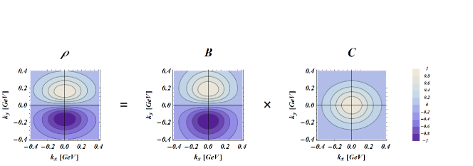
Figure 1: Simple illustration of the decomposition (12) at fixed $x$ and $\boldsymbol{b}_{T}$. The phase-space distribution $\rho$ can be written as a product of a basic multipole $B$ (here a dipole in $\boldsymbol{k}_{T}$-space) with an oval-shaped coefficient function $C$.

Table 2: Correlations between target polarization ($S_{L},\boldsymbol{S}_{T}$), quark polarization ($S^{q}_{L},\boldsymbol{S}^{q}_{T}$) and quark OAM ($\ell^{q}_{L},\boldsymbol{\ell}^{q}_{T}$) encoded in the various phase-space distributions $\rho_{X}$. We then see that e.g. $\rho_{UL}$ encodes the spin-orbit correlation $\langle S^{q}_{L}\ell^{q}_{L}\rangle$, and $\rho_{T_{x}T_{y}}$ encodes the double spin-orbit correlation $\langle S_{x}\ell^{q}_{x}S^{q}_{y}\ell^{q}_{y}\rangle$.

$\rho_{X}$	$U$	$L$	$T_{x}$	$T_{y}$
$U$	$\langle 1\rangle$	$\langle S^{q}_{L}\ell^{q}_{L}\rangle$	$\langle S^{q}_{x}\ell^{q}_{x}\rangle$	$\langle S^{q}_{y}\ell^{q}_{y}\rangle$
$L$	$\langle S_{L}\ell^{q}_{L}\rangle$	$\langle S_{L}S^{q}_{L}\rangle$	$\langle S_{L}\ell^{q}_{L}S^{q}_{x}\ell^{q}_{x}\rangle$	$\langle S_{L}\ell^{q}_{L}S^{q}_{y}\ell^{q}_{y}\rangle$
$T_{x}$	$\langle S_{x}\ell^{q}_{x}\rangle$	$\langle S_{x}\ell^{q}_{x}S^{q}_{L}\ell^{q}_{L}\rangle$	$\langle S_{x}S^{q}_{x}\rangle$	$\langle S_{x}\ell^{q}_{x}S^{q}_{y}\ell^{q}_{y}\rangle$
$T_{y}$	$\langle S_{y}\ell^{q}_{y}\rangle$	$\langle S_{y}\ell^{q}_{y}S^{q}_{L}\ell^{q}_{L}\rangle$	$\langle S_{y}\ell^{q}_{y}S^{q}_{x}\ell^{q}_{x}\rangle$	$\langle S_{y}S^{q}_{y}\rangle$

Remarkably, it turns out that all the contributions $\rho_{X}$ can be understood as encoding all the possible correlations between target and quark angular momenta, see Table 2. We stress in particular that $\vec{\ell}^{q}$ refers to the canonical quark OAM, since it is defined in terms of the canonical quark momentum $\vec{k}$ Lorce:2012ce . As will be discussed in more detail in Sec. V, the relation with all the possible angular correlations becomes more transparent once one sees the 5-dimensional relativistic phase-space distributions as 6-dimensional phase-space distributions integrated over the quark average longitudinal position

$$\rho_{X}(x,\boldsymbol{k}_{T},\boldsymbol{b}_{T};\hat{P},\eta)=\int\mathrm{d}b_{L}\,\rho_{X}(\vec{k},\vec{b};\hat{P},\eta).$$ (14)

Noting that $b_{L}$ is even under parity and odd under time-reversal, one can perform a similar multipole expansion for the 6-dimensional distributions. Naturally, the integral over $b_{L}$ of the 6-dimensional multipoles can be expressed in terms of the 5-dimensional ones

$$\int\mathrm{d}b_{L}\,\mathcal{B}(\vec{k},\vec{b};\hat{P},\eta)\,\mathcal{C}[x,\vec{k}^{2},(\vec{k}\cdot\vec{b})^{2},\vec{b}^{2},b_{L}(\vec{k}\cdot\vec{b})]=\sum_{i}B^{i}(\hat{k}_{T},\hat{b}_{T};\hat{P},\eta)\,C^{i}[x,\boldsymbol{k}^{2}_{T},(\boldsymbol{k}_{T}\cdot\boldsymbol{b}_{T})^{2},\boldsymbol{b}^{2}_{T}].$$ (15)

For convenience, this correspondence will simply be denoted in Sec. V as

$$\int\mathrm{d}b_{L}\,\mathcal{B}\sim\sum_{i}B^{i}.$$ (16)

We shall also implicitly use the fact that

$$b_{L}\,\mathcal{C}[x,\vec{k}^{2},(\vec{k}\cdot\vec{b})^{2},\vec{b}^{2},b_{L}(\vec{k}\cdot\vec{b})] =(\vec{k}\cdot\vec{b})\,\frac{b_{L}(\vec{k}\cdot\vec{b})}{(\vec{k}\cdot\vec{b})^{2}}\,\mathcal{C}[x,\vec{k}^{2},(\vec{k}\cdot\vec{b})^{2},\vec{b}^{2},b_{L}(\vec{k}\cdot\vec{b})]$$

$$\equiv(\vec{k}\cdot\vec{b})\,\mathcal{C}^{\prime}[x,\vec{k}^{2},(\vec{k}\cdot\vec{b})^{2},\vec{b}^{2},b_{L}(\vec{k}\cdot\vec{b})],$$ (17)

so that we can write e.g. $\int\mathrm{d}b_{L}\,b_{L}\sim(\hat{k}_{T}\cdot\hat{b}_{T})$. As we will explicitly show in the following, working at the level of phase-space distributions gives us much more insight about the physics encoded in the various GPDs and TMDs.

IV Representation of transverse phase space

The relativistic phase-space distributions are functions of five continuous variables. It is therefore particularly difficult to represent them on a two-dimensional space. Since we are mainly interested in the transverse direction, we reduce the number of variables by

1. integrating these phase-space distributions over $x$;

2. discretizing the polar coordinates of $\boldsymbol{b}_{T}$.

For further convenience, we also set $\eta=+1$ and choose $\hat{P}=\vec{e}_{z}=(0,0,1)$ so that $\hat{b}_{T}=(\cos\phi_{b},\sin\phi_{b},0)$ and $\hat{k}_{T}=(\cos\phi_{k},\sin\phi_{k},0)$. The resulting transverse phase-space distributions are then represented as sets of distributions in $\boldsymbol{k}_{T}$-space

$$\rho_{X}(\boldsymbol{k}_{T}|\,\boldsymbol{b}_{T})=\int\mathrm{d}x\,\rho_{X}(x,\boldsymbol{k}_{T},\boldsymbol{b}_{T};\hat{P}=\vec{e}_{z},\eta=+1)\big{|}_{\boldsymbol{b}_{T}\text{ fixed}}$$ (18)

with the origin of axes lying on circles of radius $|\boldsymbol{b}_{T}|$ at polar angle $\phi_{b}$ in impact-parameter space, see Fig. 2. In this way, one can see how the transverse momentum is distributed at some point in the impact-parameter space. In the language of differential geometry, the $\boldsymbol{b}_{T}$-space plays the role of a base space and the $\boldsymbol{k}_{T}$-space plays the role of the corresponding tangent space. All we do is just drawing the tangent spaces associated with a couple of points in the base space and situated at a fixed distance from the center. Naturally, one can also represent the same transverse phase-space distributions in terms of $\boldsymbol{b}_{T}$-distributions

$$\rho_{X}(\boldsymbol{b}_{T}|\,\boldsymbol{k}_{T})=\int\mathrm{d}x\,\rho_{X}(x,\boldsymbol{k}_{T},\boldsymbol{b}_{T};\hat{P}=\vec{e}_{z},\eta=+1)\big{|}_{\boldsymbol{k}_{T}\text{ fixed}}$$ (19)

with the origin of axes lying on circles of radius $|\boldsymbol{k}_{T}|$ at polar positions $\phi_{k}$ in transverse-momentum space. In this case, one sees how some specific transverse momentum is distributed in impact-parameter space. In the following, we shall only consider the discrete $\boldsymbol{b}_{T}$ representation $\rho_{X}(\boldsymbol{k}_{T}|\,\boldsymbol{b}_{T})$.

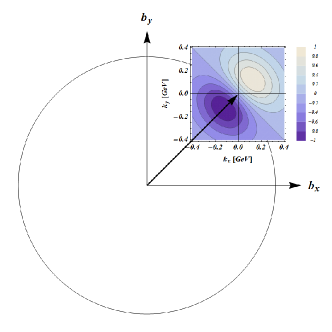
Figure 2: Representation of the transverse phase space. The circle represents the points in impact-parameter space at a fixed distance $|\boldsymbol{b}_{T}|$ from the center of the target. To each point on this circle is associated a distribution in transverse-momentum space. See text for more details.

The above representation of transverse phase space has the advantage to make the multipole structure in both $\boldsymbol{k}_{T}$ and $\boldsymbol{b}_{T}$ spaces particularly clear. For example, the basic multipole $B^{(m_{k},m_{b})}_{X}$ simply displays a $m_{k}$-pole in transverse-momentum space at any transverse position $\boldsymbol{b}_{T}$. The orientation of this $m_{k}$-pole is determined by $m_{b}$ and $\phi_{b}=\arg\hat{b}_{T}$. More precisely, by going once around the circle, the $m_{k}$-pole will undergo $\tfrac{m_{b}}{m_{k}}$ complete rotations. The case $m_{k}=0$ does not cause any problem since a monopole is invariant under rotations.

V Discussion

Since the focus of this paper is on the multipole decomposition of the transverse phase space, we choose for all the figures in the following to represent only eight points in impact-parameter space lying on a circle with radius $|\boldsymbol{b}_{T}|=0.4$ fm. Also, for a better legibility, the $\boldsymbol{k}_{T}$-distributions are normalized to the absolute maximal value over the whole circle in impact-parameter space

$$\max_{|\boldsymbol{b}_{T}|=0.4\text{ fm}}|\rho_{X}(\boldsymbol{k}_{T}|\boldsymbol{b}_{T})|=1.$$ (20)

The results presented in the following are obtained using the light-front constituent quark model (LFCQM) Lorce:2011dv for up quarks, by computing directly the Fourier transform of the helicity amplitudes associated with the GTMD correlator. Light and dark regions represent, respectively, positive and negative domains of the transverse phase-space distributions. Since our purpose at this point is simply to illustrate the multipole structure, we computed only the naive $\mathsf{T}$-even contributions in this model. The fact that the calculated distributions perfectly match the expected multipole decomposition presented in Sec. III proves the consistency of the approach. The naive $\mathsf{T}$-odd contributions have been obtained by extracting the coefficient functions from the naive $\mathsf{T}$-even part and multiplying them by the appropriate basic multipoles. We stress that the global sign of these naive $\mathsf{T}$-odd contributions has been chosen arbitrarily. Only a proper calculation including initial- and/or final-state interactions can determine these global signs.

V.1 Unpolarized target

V.1.1 Unpolarized quark

The simplest contribution is $\rho_{UU}$. It describes the distribution of unpolarized quarks inside an unpolarized target. As already discussed at the end of Sec. III, there exist only two spin-independent phase-space distributions

$$\rho^{e}_{UU}=\rho^{(0,0)}_{UU},\qquad\rho^{o}_{UU}=\rho^{(1,1)}_{UU},$$ (21)

which are represented in Fig. 3.

             

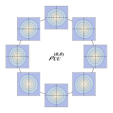
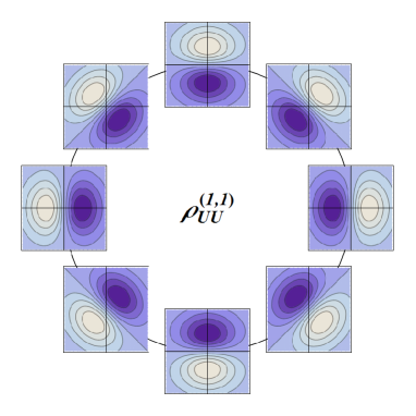
Figure 3: Naive $\mathsf{T}$-even (left) and $\mathsf{T}$-odd (right) contributions to the transverse phase-space distribution $\rho_{UU}$. See text for more details.

The corresponding basic multipoles are

$$B^{(0,0)}_{UU}(\hat{k}_{T},\hat{b}_{T};\hat{P},\eta) =M_{k}M_{b}=1,$$ (22)

$$B^{(1,1)}_{UU}(\hat{k}_{T},\hat{b}_{T};\hat{P},\eta) =\eta\,D^{i}_{k}D^{i}_{b}=\eta\,(\hat{k}_{T}\cdot\hat{b}_{T}).$$ (23)

Only $\rho^{(0,0)}_{UU}$ survives integration over $\boldsymbol{k}_{T}$ or $\boldsymbol{b}_{T}$ and is then naturally related to both the unpolarized GPD $H$ and the unpolarized TMD $f_{1}$ Diehl:2005jf ; Lorce:2011dv . Contrary to its $\boldsymbol{k}_{T}$- and $\boldsymbol{b}_{T}$-integrated versions, $\rho^{(0,0)}_{UU}$ is not circularly symmetric. The reason is that $\rho^{(0,0)}_{UU}$ also contains information about the correlation between $\boldsymbol{k}_{T}$ and $\boldsymbol{b}_{T}$, which is lost under integration over one of the transverse variables Lorce:2011kd . As one can see from Fig. 3, the $\boldsymbol{k}_{T}$-distribution is elongated in the direction orthogonal to the transverse position. This means that a polar flow ($\boldsymbol{k}_{T}\perp\boldsymbol{b}_{T}$) is preferred over a radial flow ($\boldsymbol{k}_{T}\parallel\boldsymbol{b}_{T}$), which is expected because the quarks are bound in the target. In other words, the preferred flow of quarks is along circles around the center of the target. The quark motion is of course not limited to the transverse plane. So, for fixed quark momentum $\vec{k}$, $\rho^{(0,0)}_{UU}$ should better be thought of as the projection of a 3-dimensional distribution in position space onto the transverse plane

$$\int\mathrm{d}b_{L}\,1\sim 1.$$ (24)

Note however that the net OAM is zero in this case, because there is no preferred direction in $\rho_{UU}$. Quarks tend to follow circular motion equally in both clockwise and anti-clockwise directions.

Since it integrates to zero in both $\boldsymbol{k}_{T}$ and $\boldsymbol{b}_{T}$-spaces, $\rho^{(1,1)}_{UU}$ represents a completely new piece of information which is not accessible via GPDs or TMDs at leading twist. The dipole in $\boldsymbol{k}_{T}$-space signals the presence of a net flow in the transverse radial direction $(\hat{k}_{T}\cdot\hat{b}_{T})$, which can be seen as the projection of a 3-dimensional radial flow $(\hat{k}\cdot\hat{b})$ onto the transverse position space

$$\int\mathrm{d}b_{L}\,(\vec{k}\cdot\vec{b})\sim(\hat{k}_{T}\cdot\hat{b}_{T}).$$ (25)

For a stable target, this must obviously be zero. A non-vanishing net radial flow therefore originates purely from initial- and final-state interactions, in agreement with the naive $\mathsf{T}$-odd nature of $\rho^{(1,1)}_{UU}$. The coefficient function $C^{(1,1)}_{UU}$ then represents in some sense the strength of the spin-independent part of the force felt by the quark due to initial- and final-state interactions.

V.1.2 Longitudinally polarized quark

The contribution $\rho_{UL}$ describes how the distribution of quarks inside an unpolarized target is affected by the quark longitudinal polarization. We find only two phase-space distributions

$$\rho^{e}_{UL}=\rho^{(1,1)}_{UL},\qquad\rho^{o}_{UL}=\rho^{(2,2)}_{UL},$$ (26)

which are represented in Fig. 4.

             

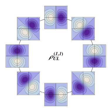
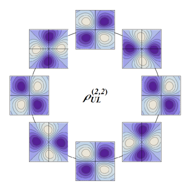
Figure 4: Naive $\mathsf{T}$-even (left) and $\mathsf{T}$-odd (right) contributions to the transverse phase-space distribution $\rho_{UL}$. See text for more details.

The corresponding basic multipoles are

$$S^{q}_{L}\,B^{(1,1)}_{UL}(\hat{k}_{T},\hat{b}_{T};\hat{P},\eta) =-S^{q}_{L}\epsilon^{ij}_{T}D^{i}_{k}D^{j}_{b}=S^{q}_{L}(\hat{b}_{T}\times\hat{k}_{T})_{L},$$ (27)

$$S^{q}_{L}\,B^{(2,2)}_{UL}(\hat{k}_{T},\hat{b}_{T};\hat{P},\eta) =-\eta\,S^{q}_{L}\epsilon^{ij}_{T}Q^{il}_{k}Q^{jl}_{b}=\eta\,S^{q}_{L}(\hat{b}_{T}\times\hat{k}_{T})_{L}\,(\hat{k}_{T}\cdot\hat{b}_{T}).$$ (28)

None of these survive integration over $\boldsymbol{k}_{T}$ or $\boldsymbol{b}_{T}$. Both therefore represent completely new information which is not accessible via GPDs or TMDs at leading twist. The $\boldsymbol{k}_{T}$-dipole in $\rho^{(1,1)}_{UL}$ signals the presence of a net flow in the polar direction $(\hat{b}_{T}\times\hat{k}_{T})_{L}$, i.e. a net longitudinal component of quark OAM, which can be seen as the projection of a 3-dimensional azimuthal flow $(\vec{b}\times\vec{k})\cdot\hat{P}$ onto the transverse position space

$$\int\mathrm{d}b_{L}\,[(\vec{b}\times\vec{k})\cdot\hat{P}]\sim(\hat{b}_{T}\times\hat{k}_{T})_{L}.$$ (29)

By reversing the quark longitudinal polarization $S^{q}_{L}$, one reverses also the orbital flow. The coefficient function $C^{(1,1)}_{UL}$ then represents in some sense the strength of the correlation between the longitudinal components of quark polarization and OAM $\langle S^{q}_{L}\ell^{q}_{L}\rangle$ Lorce:2011kd ; Lorce:2014mxa .

On the contrary, the contribution $\rho^{(2,2)}_{UL}$ does not modify the net quark flow. The effect of the $\boldsymbol{k}_{T}$-quadrupoles is to globally tilt the $\boldsymbol{k}_{T}$-distributions with respect to $\boldsymbol{b}_{T}$, so that the preferred flow is now a spiral correlated with the quark longitudinal polarization, which can be seen as the projection of a 3-dimensional spiral flow onto the transverse position space

$$\int\mathrm{d}b_{L}\,[(\vec{b}\times\vec{k})\cdot\hat{P}]\,(\vec{k}\cdot\vec{b})\sim(\hat{b}_{T}\times\hat{k}_{T})_{L}\,(\hat{k}_{T}\cdot\hat{b}_{T}).$$ (30)

In other words, the contribution $\rho^{(2,2)}_{UL}$ gives the difference of radial flows between quarks with opposite $\langle S^{q}_{L}\ell^{q}_{L}\rangle$ correlations. The coefficient function $C^{(2,2)}_{UL}$ then represents in some sense the strength of the $\langle S^{q}_{L}\ell^{q}_{L}\rangle$-dependent part of the force felt by the quark due to initial- and final-state interactions.

V.1.3 Transversely polarized quark

The contribution $\rho_{UT^{i}}$ describes how the distribution of quarks inside an unpolarized target is affected by the quark transverse polarization. We find in total four phase-space distributions

$$\rho^{e}_{UT^{i}}=\rho^{(0,1)}_{UT^{i}}+\rho^{(2,1)}_{UT^{i}},\qquad\rho^{o}_{UT^{i}}=\rho^{(1,0)}_{UT^{i}}+\rho^{(1,2)}_{UT^{i}},$$ (31)

which are represented in Fig. 5 for the quark polarization $\vec{S}^{q}_{T}=\vec{e}_{x}$.

             

             

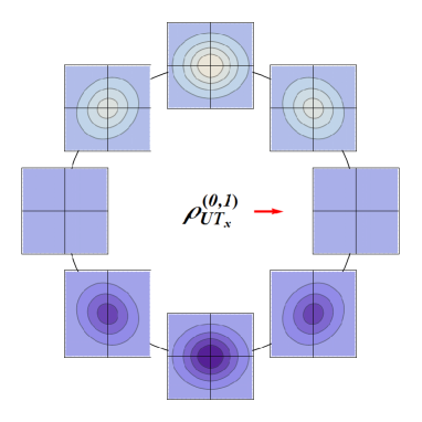
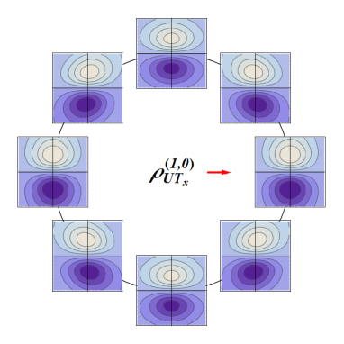
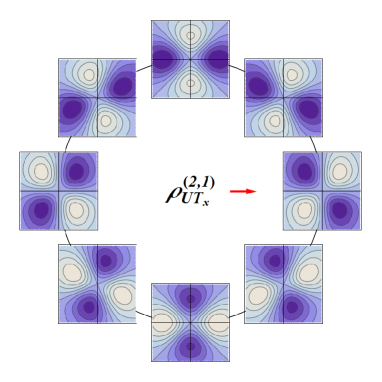
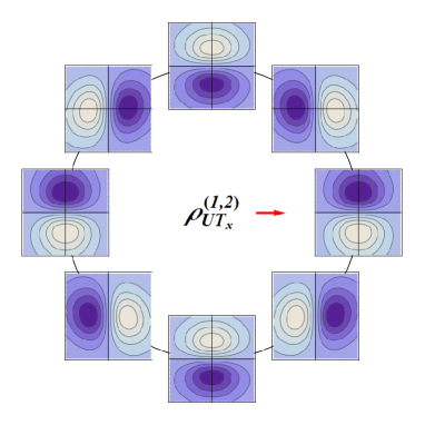
Figure 5: Naive $\mathsf{T}$-even (left) and $\mathsf{T}$-odd (right) contributions to the transverse phase-space distribution $\rho_{UT}$ for the quark polarization $\vec{S}^{q}_{T}=\vec{e}_{x}$ (red arrow). See text for more details.

The corresponding basic multipoles are

$$S^{qi}_{T}\,B^{(0,1)}_{UT^{i}}(\hat{k}_{T},\hat{b}_{T};\hat{P},\eta) =S^{qi}_{T}\epsilon^{ij}_{T}M_{k}D^{j}_{b}=(\boldsymbol{S}^{q}_{T}\times\hat{b}_{T})_{L},$$ (32)

$$S^{qi}_{T}\,B^{(2,1)}_{UT^{i}}(\hat{k}_{T},\hat{b}_{T};\hat{P},\eta) =S^{qi}_{T}\epsilon^{ij}_{T}Q^{jl}_{k}D^{l}_{b}=(\boldsymbol{S}^{q}_{T}\times\hat{k}_{T})_{L}\,(\hat{k}_{T}\cdot\hat{b}_{T})-\tfrac{1}{2}\,(\boldsymbol{S}^{q}_{T}\times\hat{b}_{T})_{L},$$ (33)

$$S^{qi}_{T}\,B^{(1,0)}_{UT^{i}}(\hat{k}_{T},\hat{b}_{T};\hat{P},\eta) =\eta\,S^{qi}_{T}\epsilon^{ij}_{T}D^{j}_{k}M_{b}=\eta\,(\boldsymbol{S}^{q}_{T}\times\hat{k}_{T})_{L},$$ (34)

$$S^{qi}_{T}\,B^{(1,2)}_{UT^{i}}(\hat{k}_{T},\hat{b}_{T};\hat{P},\eta) =\eta\,S^{qi}_{T}\epsilon^{jl}_{T}D^{l}_{k}Q^{ij}_{b}=\eta\left[(\boldsymbol{S}^{q}_{T}\cdot\hat{b}_{T})\,(\hat{b}_{T}\times\hat{k}_{T})_{L}-\tfrac{1}{2}\,(\boldsymbol{S}^{q}_{T}\times\hat{k}_{T})_{L}\right].$$ (35)

The contribution $\rho^{(0,1)}_{UT^{i}}$ is the only one surviving the integration over $\boldsymbol{k}_{T}$ and is then naturally related to the GPD combination $2\tilde{H}_{T}+E_{T}$ Diehl:2005jf ; Lorce:2011dv ; Pasquini:2007xz . The dipole in $\boldsymbol{b}_{T}$-space indicates the presence of a spatial separation between quarks with opposite transverse polarizations. This transverse shift is actually an effect related to the light-front imaging due to the fact that the light-front densities are defined in terms of the $j^{+}=\tfrac{1}{\sqrt{2}}(j^{0}+j^{3})$ component of the current instead of the $j^{0}$ component, and finds its physical origin in the correlation between the transverse components of quark polarization and OAM $\langle\boldsymbol{S}^{q}_{T}\cdot\boldsymbol{\ell}^{q}_{T}\rangle$ Burkardt:2005hp . Indeed, because of transverse OAM, quarks situated at opposite sides tend to have opposite longitudinal momenta $k_{L}\,\hat{P}$, i.e. opposite $j^{3}$ components, and are then associated with different light-front densities $j^{+}$. From a slightly different perspective, the transverse shift can also be understood from the fact that the position of the relativistic center-of-mass of a rotating body is frame-dependent Moller:1949 ; Moller:1972 .

There are actually two independent transverse correlations, say $\langle S^{q}_{x}\ell^{q}_{x}\rangle$ and $\langle S^{q}_{y}\ell^{q}_{y}\rangle$. The contribution $\rho^{(0,1)}_{UT^{i}}$ gives us information about only one particular combination. The other combination is given by the other naive $\mathsf{T}$-even contribution $\rho^{(2,1)}_{UT^{i}}$ which is not accessible via GPDs or TMDs at leading twist. Indeed, let us consider the projection of a 3-dimensional $\langle(\vec{S}^{q}_{T}\cdot\vec{n}_{T})(\vec{\ell}^{q}_{T}\cdot\vec{n}_{T})\rangle$ correlation onto the transverse position space, where $\vec{n}_{T}$ is some transverse vector. For $\vec{n}_{T}=\vec{k}_{T}$ and $\vec{n}_{T}=(\vec{k}_{T}\times\hat{P})$, we respectively find

$$\int\mathrm{d}b_{L}\,(\vec{S}^{q}_{T}\cdot\vec{k}_{T})\,[(\vec{b}\times\vec{k})_{T}\cdot\vec{k}_{T}] \sim(\boldsymbol{S}^{q}_{T}\cdot\hat{k}_{T})\,(\hat{k}_{T}\times\hat{b}_{T})_{L},$$ (36)

$$\int\mathrm{d}b_{L}\,[\vec{S}^{q}_{T}\cdot(\vec{k}_{T}\times\hat{P})]\,[(\vec{b}\times\vec{k})_{T}\cdot(\vec{k}_{T}\times\hat{P})] \sim(\boldsymbol{S}^{q}_{T}\times\hat{k}_{T})_{L}\,(\hat{k}_{T}\cdot\hat{b}_{T}).$$ (37)

Noting that

$$(\boldsymbol{S}^{q}_{T}\cdot\hat{k}_{T})\,(\hat{k}_{T}\times\hat{b}_{T})_{L}+(\boldsymbol{S}^{q}_{T}\times\hat{k}_{T})_{L}\,(\hat{k}_{T}\cdot\hat{b}_{T})=(\boldsymbol{S}^{q}_{T}\times\hat{b}_{T})_{L}$$ (38)

and comparing with the basic multipoles (32) and (33), we can see that the two coefficient functions $C^{(0,1)}_{UT^{i}}$ and $C^{(2,1)}_{UT^{i}}$ are related to the strength of two different combinations of the transverse correlations $\langle S^{q}_{x}\ell^{q}_{x}\rangle$ and $\langle S^{q}_{y}\ell^{q}_{y}\rangle$.

Similarly, the contribution $\rho^{(1,0)}_{UT^{i}}$ is the only one surviving the integration over $\boldsymbol{b}_{T}$ and is then naturally related to the Boer-Mulders TMD $h^{\perp}_{1}$. The dipole in $\boldsymbol{k}_{T}$-space indicates the presence of a net transverse flow orthogonal to the quark transverse polarization. Interestingly, this phenomenon is reminiscent of the spin Hall effect in spintronics and the Magnus effect in fluid mechanics Dyakonov:1971a ; Dyakonov:1971b . Such a net transverse flow can only arise from initial- and/or final-state interactions, in accordance with the naive $\mathsf{T}$-odd nature of $\rho^{(1,0)}_{UT^{i}}$.

The contribution $\rho^{(1,2)}_{UT^{i}}$ corresponds to a completely new information which is not accessible via GPDs or TMDs at leading twist. Combined with $\rho^{(1,0)}_{UT^{i}}$, it tells us how the initial- and final-state interactions depend on the two transverse correlations, say $\langle S^{q}_{x}\ell^{q}_{x}\rangle$ and $\langle S^{q}_{y}\ell^{q}_{y}\rangle$. Indeed, let us consider the projection of a 3-dimensional transverse spiral flow $(\vec{S}^{q}_{T}\cdot\vec{n}_{T})\,[(\vec{b}\times\vec{k})_{T}\cdot\vec{n}_{T}]\,(\vec{k}\cdot\vec{b})$ onto the transverse position space. For $\vec{n}_{T}=\vec{b}_{T}$ and $\vec{n}_{T}=(\vec{b}_{T}\times\hat{P})$, we respectively find

$$\int\mathrm{d}b_{L}\,(\vec{S}^{q}_{T}\cdot\vec{b}_{T})\,[(\vec{b}\times\vec{k})_{T}\cdot\vec{b}_{T}]\,(\vec{k}\cdot\vec{b}) \sim(\boldsymbol{S}^{q}_{T}\cdot\hat{b}_{T})\,(\hat{b}_{T}\times\hat{k}_{T})_{L},$$ (39)

$$\int\mathrm{d}b_{L}\,[\vec{S}^{q}_{T}\cdot(\vec{b}_{T}\times\hat{P})]\,[(\vec{b}\times\vec{k})_{T}\cdot(\vec{b}_{T}\times\hat{P})]\,(\vec{k}\cdot\vec{b}) \sim(\boldsymbol{S}^{q}_{T}\times\hat{b}_{T})_{L}\,(\hat{b}_{T}\cdot\hat{k}_{T}).$$ (40)

Noting that

$$(\boldsymbol{S}^{q}_{T}\cdot\hat{b}_{T})\,(\hat{b}_{T}\times\hat{k}_{T})_{L}+(\boldsymbol{S}^{q}_{T}\times\hat{b}_{T})_{L}\,(\hat{b}_{T}\cdot\hat{k}_{T})=(\boldsymbol{S}^{q}_{T}\times\hat{k}_{T})_{L}$$ (41)

and comparing with the basic multipoles (34) and (35), we can see that the two coefficient functions $C^{(1,0)}_{UT^{i}}$ and $C^{(1,2)}_{UT^{i}}$ are related to the strength of the $\langle S^{q}_{x}\ell^{q}_{x}\rangle$- and $\langle S^{q}_{y}\ell^{q}_{y}\rangle$-dependent parts of the force felt by the quark due to initial- and final-state interactions. In other words, the contributions $\rho^{(1,0)}_{UT^{i}}$ and $\rho^{(1,2)}_{UT^{i}}$ describe the difference of radial flows between quarks with opposite $\langle S^{q}_{x}\ell^{q}_{x}\rangle$ or $\langle S^{q}_{y}\ell^{q}_{y}\rangle$ correlations.

As a final remark, it has been suggested by Burkardt Burkardt:2005hp that $\int\mathrm{d}^{2}k_{T}\,\rho^{e}_{UT^{i}}$ and $\int\mathrm{d}^{2}b_{T}\,\rho^{o}_{UT^{i}}$ could be related by some lensing effect. We cannot unfortunately confirm this suggestion, because such a relation relies on a dynamical mechanism which goes beyond the general constraints considered in the present paper.

V.2 Longitudinally polarized target

V.2.1 Unpolarized quark

The contribution $\rho_{LU}$ describes how the distribution of unpolarized quarks is affected by the target longitudinal polarization. Its structure is very similar to $\rho_{UL}$ because one just exchanges the roles of quark and target polarizations. We then find only two phase-space distributions

$$\rho^{e}_{LU}=\rho^{(1,1)}_{LU},\qquad\rho^{o}_{LU}=\rho^{(2,2)}_{LU},$$ (42)

which are represented in Fig. 6. None of these survive integration over $\boldsymbol{k}_{T}$ or $\boldsymbol{b}_{T}$. Both therefore represent completely new information which is not accessible via GPDs or TMDs at leading twist.

Following the same arguments as in Sec. V.1.2, with $S_{L}^{q}$ replaced by $S_{L}$, we can relate the $\rho^{(1,1)}_{LU}$ contribution to the presence of a net longitudinal component of quark OAM correlated with the target longitudinal polarization $S_{L}$, with the coefficient function $C^{(1,1)}_{LU}$ giving the amount of longitudinal quark OAM in a longitudinally polarized target $\langle S_{L}\ell^{q}_{L}\rangle$ Lorce:2011kd . Similarly, the contribution $\rho^{(2,2)}_{LU}$ gives the difference of radial flows between quarks with opposite OAM $\langle S_{L}\ell^{q}_{L}\rangle$, with the coefficient function $C^{(2,2)}_{LU}$ representing in some sense the strength of the $\langle S_{L}\ell^{q}_{L}\rangle$-dependent part of the force felt by the quark due to initial- and final-state interactions.

             

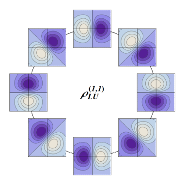
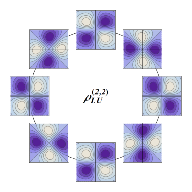
Figure 6: Naive $\mathsf{T}$-even (left) and $\mathsf{T}$-odd (right) contributions to the transverse phase-space distribution $\rho_{LU}$. See text for more details.

The corresponding basic multipoles are

$$S_{L}\,B^{(1,1)}_{LU}(\hat{k}_{T},\hat{b}_{T};\hat{P},\eta) =-S_{L}\epsilon^{ij}_{T}D^{i}_{k}D^{j}_{b}=S_{L}(\hat{b}_{T}\times\hat{k}_{T})_{L},$$ (43)

$$S_{L}\,B^{(2,2)}_{LU}(\hat{k}_{T},\hat{b}_{T};\hat{P},\eta) =-\eta\,S_{L}\epsilon^{ij}_{T}Q^{il}_{k}Q^{jl}_{b}=\eta\,S_{L}(\hat{b}_{T}\times\hat{k}_{T})_{L}\,(\hat{k}_{T}\cdot\hat{b}_{T}).$$ (44)

V.2.2 Longitudinally polarized quark

The contribution $\rho_{LL}$ describes how the quark distribution is affected by the correlation between the quark and target longitudinal polarizations. Since the product $S_{L}S^{q}_{L}$ is invariant under parity and time-reversal, the contribution $\rho_{LL}$ turns out to be very similar to $\rho_{UU}$. We then find only two phase-space distributions

$$\rho^{e}_{LL}=\rho^{(0,0)}_{LL},\qquad\rho^{o}_{LL}=\rho^{(1,1)}_{LL},$$ (45)

which are represented in Fig. 7. The corresponding basic multipoles are

$$S_{L}S^{q}_{L}\,B^{(0,0)}_{LL}(\hat{k}_{T},\hat{b}_{T};\hat{P},\eta) =S_{L}S^{q}_{L}M_{k}M_{b}=S_{L}S^{q}_{L},$$ (46)

$$S_{L}S^{q}_{L}\,B^{(1,1)}_{LL}(\hat{k}_{T},\hat{b}_{T};\hat{P},\eta) =\eta\,S_{L}S^{q}_{L}D^{i}_{k}D^{i}_{b}=\eta\,S_{L}S^{q}_{L}(\hat{k}_{T}\cdot\hat{b}_{T}).$$ (47)

Only $\rho^{(0,0)}_{LL}$ survives integration over $\boldsymbol{k}_{T}$ or $\boldsymbol{b}_{T}$ and is then naturally related to both the helicity GPD $\tilde{H}$ and the helicity TMD $g_{1L}$ Diehl:2005jf ; Lorce:2011dv . Contrary to its $\boldsymbol{k}_{T}$- and $\boldsymbol{b}_{T}$-integrated versions, $\rho^{(0,0)}_{LL}$ is not circularly symmetric. The reason is that $\rho^{(0,0)}_{LL}$ also contains information about the correlation between $\boldsymbol{k}_{T}$ and $\boldsymbol{b}_{T}$, which is lost under integration over one of the transverse variables Lorce:2011kd .
Following the same arguments as in Sec. V.1.1, with now all expressions multiplied by $S_{L}S_{L}^{q}$, we can relate the coefficient function $C^{(0,0)}_{LL}$ to the strength of the correlation between the longitudinal component of quark and target polarizations $\langle S_{L}S^{q}_{L}\rangle$. Similarly, the contribution $\rho^{(1,1)}_{LL}$ gives the difference of radial flows between quarks with opposite $\langle S_{L}S^{q}_{L}\rangle$ correlations, with the coefficient function $C^{(1,1)}_{LL}$ representing in some sense the strength of the $\langle S_{L}S^{q}_{L}\rangle$-dependent part of the force felt by the quark due to initial- and final-state interactions.

V.2.3 Transversely polarized quark

             

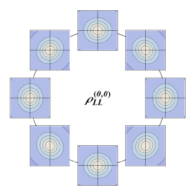
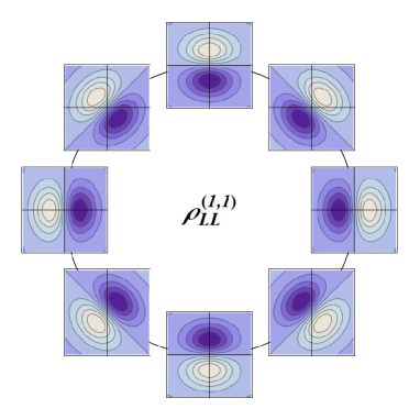
Figure 7: Naive $\mathsf{T}$-even (left) and $\mathsf{T}$-odd (right) contributions to the transverse phase-space distribution $\rho_{LL}$. See text for more details.

The contribution $\rho_{LT^{i}}$ describes how the distribution of quarks is affected by the combination of quark transverse polarization and target longitudinal polarization. We find in total four phase-space distributions

$$\rho^{e}_{LT^{i}}=\rho^{(1,0)}_{LT^{i}}+\rho^{(1,2)}_{LT^{i}},\qquad\rho^{o}_{LT^{i}}=\rho^{(0,1)}_{LT^{i}}+\rho^{(2,1)}_{LT^{i}},$$ (48)

which are represented in Fig. 8 for the quark polarization $\vec{S}^{q}_{T}=\vec{e}_{x}$.

             

             

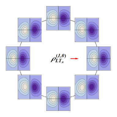
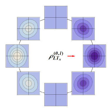
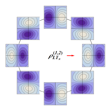
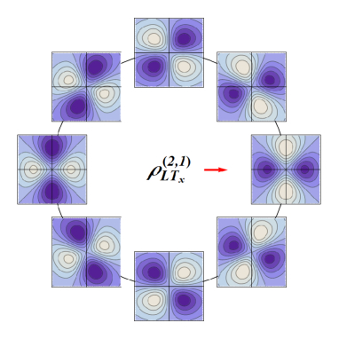
Figure 8: Naive $\mathsf{T}$-even (left) and $\mathsf{T}$-odd (right) contributions to the transverse phase-space distribution $\rho_{LT}$ for the quark polarization $\vec{S}^{q}_{T}=\vec{e}_{x}$ (red arrow). See text for more details.

The corresponding basic multipoles are

$$S_{L}S^{qi}_{T}\,B^{(1,0)}_{LT^{i}}(\hat{k}_{T},\hat{b}_{T};\hat{P},\eta) =S_{L}S^{qi}_{T}D^{i}_{k}M_{b}=S_{L}(\boldsymbol{S}^{q}_{T}\cdot\hat{k}_{T}),$$ (49)

$$S_{L}S^{qi}_{T}\,B^{(1,2)}_{LT^{i}}(\hat{k}_{T},\hat{b}_{T};\hat{P},\eta) =S_{L}S^{qi}_{T}D^{j}_{k}Q^{ij}_{b}=S_{L}\!\left[(\boldsymbol{S}^{q}_{T}\cdot\hat{b}_{T})\,(\hat{b}_{T}\cdot\hat{k}_{T})-\tfrac{1}{2}\,(\boldsymbol{S}^{q}_{T}\cdot\hat{k}_{T})\right],$$ (50)

$$S_{L}S^{qi}_{T}\,B^{(0,1)}_{LT^{i}}(\hat{k}_{T},\hat{b}_{T};\hat{P},\eta) =\eta\,S_{L}S^{qi}_{T}M_{k}D^{i}_{b}=\eta\,S_{L}(\boldsymbol{S}^{q}_{T}\cdot\hat{b}_{T}),$$ (51)

$$S_{L}S^{qi}_{T}\,B^{(2,1)}_{LT^{i}}(\hat{k}_{T},\hat{b}_{T};\hat{P},\eta) =\eta\,S_{L}S^{qi}_{T}Q^{ij}_{k}D^{j}_{b}=\eta\,S_{L}\!\left[(\boldsymbol{S}^{q}_{T}\cdot\hat{k}_{T})\,(\hat{k}_{T}\cdot\hat{b}_{T})-\tfrac{1}{2}\,(\boldsymbol{S}^{q}_{T}\cdot\hat{b}_{T})\right].$$ (52)

The contribution $\rho^{(1,0)}_{LT^{i}}$ is the only one surviving the integration over $\boldsymbol{b}_{T}$ and is then naturally related to the worm-gear TMD $h^{\perp}_{1L}$ Diehl:2005jf ; Lorce:2011dv . The dipole in $\boldsymbol{k}_{T}$-space indicates the presence of a net transverse flow parallel to the quark transverse polarization. This transverse flow is actually an effect due to the light-front imaging, once again associated with the fact that the light-front densities are defined in terms of the $j^{+}=\tfrac{1}{\sqrt{2}}(j^{0}+j^{3})$ component of the current instead of the $j^{0}$ component. As we will soon see, it turns out that the transverse flow finds its physical origin in the correlation between the longitudinal component of quark OAM and the transverse spin-orbit coupling $\langle S_{L}\ell^{q}_{L}(\boldsymbol{S}^{q}_{T}\cdot\boldsymbol{\ell}^{q}_{T})\rangle$.

The contribution $\rho^{(1,2)}_{LT^{i}}$ corresponds to a completely new information which is not accessible via GPDs or TMDs at leading twist. Combined with $\rho^{(1,0)}_{LT^{i}}$, it tells us how the quark distribution is affected by the two longitudinal-transverse worm-gear correlations, say $\langle S_{L}\ell^{q}_{L}S^{q}_{x}\ell^{q}_{x}\rangle$ and $\langle S_{L}\ell^{q}_{L}S^{q}_{y}\ell^{q}_{y}\rangle$. Indeed, let us consider the projection of a 3-dimensional $\langle S_{L}\ell^{q}_{L}(\vec{S}^{q}_{T}\cdot\vec{n}_{T})(\vec{\ell}^{q}_{T}\cdot\vec{n}_{T})\rangle$ correlation onto the transverse position space. For $\vec{n}_{T}=\vec{b}_{T}$ and $\vec{n}_{T}=(\vec{b}_{T}\times\hat{P})$, we respectively find

$$\int\mathrm{d}b_{L}\,[(\vec{b}\times\vec{k})\cdot\hat{P}]\,(\vec{S}^{q}_{T}\cdot\vec{b}_{T})\,[(\vec{b}\times\vec{k})_{T}\cdot\vec{b}_{T}] \sim(\boldsymbol{S}^{q}_{T}\cdot\hat{b}_{T})\,(\hat{b}_{T}\cdot\hat{k}_{T}),$$ (53)

$$\int\mathrm{d}b_{L}\,[(\vec{b}\times\vec{k})\cdot\hat{P}]\,[\vec{S}^{q}_{T}\cdot(\vec{b}_{T}\times\hat{P})]\,[(\vec{b}\times\vec{k})_{T}\cdot(\vec{b}_{T}\times\hat{P})] \sim(\boldsymbol{S}^{q}_{T}\times\hat{b}_{T})_{L}\,(\hat{b}_{T}\times\hat{k}_{T})_{L}.$$ (54)

Noting that

$$(\boldsymbol{S}^{q}_{T}\cdot\hat{b}_{T})\,(\hat{b}_{T}\cdot\hat{k}_{T})-(\boldsymbol{S}^{q}_{T}\times\hat{b}_{T})_{L}\,(\hat{b}_{T}\times\hat{k}_{T})_{L}=(\boldsymbol{S}^{q}_{T}\cdot\hat{k}_{T})$$ (55)

and comparing with the basic multipoles (49) and (50), we can see that the two coefficient functions $C^{(1,0)}_{LT^{i}}$ and $C^{(1,2)}_{LT^{i}}$ are related to the strength of two different combinations of the two longitudinal-transverse worm-gear correlations $\langle S_{L}\ell^{q}_{L}S^{q}_{x}\ell^{q}_{x}\rangle$ and $\langle S_{L}\ell^{q}_{L}S^{q}_{y}\ell^{q}_{y}\rangle$.

Similarly, the contribution $\rho^{(0,1)}_{LT^{i}}$ is the only one surviving the integration over $\boldsymbol{k}_{T}$. It cannot however be related to the GPD $\tilde{E}_{T}$ Diehl:2005jf ; Lorce:2011dv ; Pasquini:2007xz since the latter is $\eta$-independent. It then corresponds to a completely new information. Once again, the dipole in $\boldsymbol{b}_{T}$-space indicates the presence of a spatial separation between quarks with opposite correlations. This is again an effect related to the light-front imaging.

The contribution $\rho^{(2,1)}_{LT^{i}}$ corresponds to another completely new information which is not accessible via GPDs or TMDs at leading twist. Combined with $\rho^{(0,1)}_{LT^{i}}$, it tells us how the initial- and final state-interactions depend on the two longitudinal-transverse worm-gear correlations, say $\langle S_{L}\ell^{q}_{L}S^{q}_{x}\ell^{q}_{x}\rangle$ and $\langle S_{L}\ell^{q}_{L}S^{q}_{y}\ell^{q}_{y}\rangle$. Indeed, let us consider the projection of a 3-dimensional spiral worm-gear flow $[(\vec{b}\times\vec{k})\cdot\hat{P}]\,(\vec{S}^{q}_{T}\cdot\vec{n}_{T})\,[(\vec{b}\times\vec{k})_{T}\cdot\vec{n}_{T}]\,(\vec{k}\cdot\vec{b})$ onto the transverse position space. For $\vec{n}_{T}=\vec{k}_{T}$ and $\vec{n}_{T}=(\vec{k}_{T}\times\hat{P})$, we respectively find

$$\int\mathrm{d}b_{L}\,[(\vec{b}\times\vec{k})\cdot\hat{P}]\,(\vec{S}^{q}_{T}\cdot\vec{k}_{T})\,[(\vec{b}\times\vec{k})_{T}\cdot\vec{k}_{T}]\,(\vec{k}\cdot\vec{b}) \sim(\boldsymbol{S}^{q}_{T}\cdot\hat{k}_{T})\,(\hat{k}_{T}\cdot\hat{b}_{T}),$$ (56)

$$\int\mathrm{d}b_{L}\,[(\vec{b}\times\vec{k})\cdot\hat{P}]\,[\vec{S}^{q}_{T}\cdot(\vec{k}_{T}\times\hat{P})]\,[(\vec{b}\times\vec{k})_{T}\cdot(\vec{k}_{T}\times\hat{P})]\,(\vec{k}\cdot\vec{b}) \sim(\boldsymbol{S}^{q}_{T}\times\hat{k}_{T})_{L}\,(\hat{k}_{T}\times\hat{b}_{T})_{L}.$$ (57)

Noting that

$$(\boldsymbol{S}^{q}_{T}\cdot\hat{k}_{T})\,(\hat{k}_{T}\cdot\hat{b}_{T})-(\boldsymbol{S}^{q}_{T}\times\hat{k}_{T})_{L}\,(\hat{k}_{T}\times\hat{b}_{T})_{L}=(\boldsymbol{S}^{q}_{T}\cdot\hat{b}_{T})$$ (58)

and comparing with the basic multipoles (51) and (52), we can see that the two coefficient functions $C^{(0,1)}_{LT^{i}}$ and $C^{(2,1)}_{LT^{i}}$ are related to the strength of the $\langle S_{L}\ell^{q}_{L}S^{q}_{x}\ell^{q}_{x}\rangle$- and $\langle S_{L}\ell^{q}_{L}S^{q}_{y}\ell^{q}_{y}\rangle$-dependent parts of the force felt by the quark due to initial and final-state interactions. In other words, the contributions $\rho^{(0,1)}_{LT^{i}}$ and $\rho^{(2,1)}_{LT^{i}}$ describe the difference of radial flows between quarks with opposite $\langle S_{L}\ell^{q}_{L}S^{q}_{x}\ell^{q}_{x}\rangle$ or $\langle S_{L}\ell^{q}_{L}S^{q}_{y}\ell^{q}_{y}\rangle$ correlations.

V.3 Transversely polarized target

V.3.1 Unpolarized quark

The contribution $\rho_{T^{i}U}$ describes how the distribution of unpolarized quarks is affected by the target transverse polarization. Its structure is very similar to $\rho_{UT^{i}}$ because one just exchanges the roles of quark and target polarizations. We then find in total four phase-space distributions

$$\rho^{e}_{T^{i}U}=\rho^{(0,1)}_{T^{i}U}+\rho^{(2,1)}_{T^{i}U},\qquad\rho^{o}_{T^{i}U}=\rho^{(1,0)}_{T^{i}U}+\rho^{(1,2)}_{T^{i}U},$$ (59)

which are represented in Fig. 9 for the target polarization $\vec{S}_{T}=\vec{e}_{x}$.

             

             

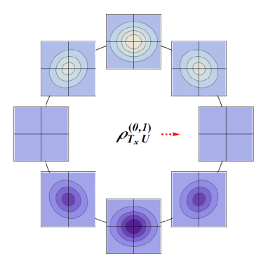
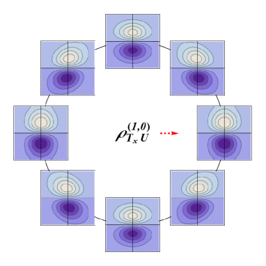
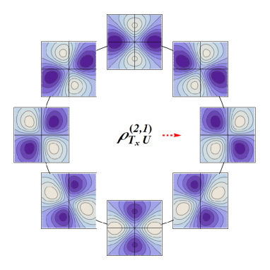
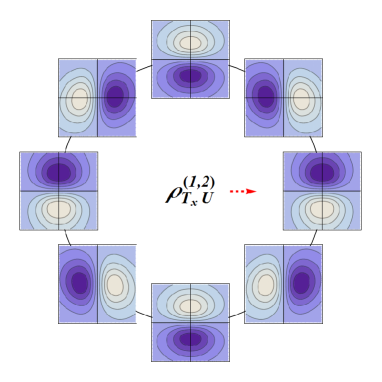
Figure 9: Naive $\mathsf{T}$-even (left) and $\mathsf{T}$-odd (right) contributions to the transverse phase-space distribution $\rho_{TU}$ for the target polarization $\vec{S}_{T}=\vec{e}_{x}$ (red dashed arrow). See text for more details.

The corresponding basic multipoles are

$$S^{i}_{T}\,B^{(0,1)}_{T^{i}U}(\hat{k}_{T},\hat{b}_{T};\hat{P},\eta) =S^{i}_{T}\epsilon^{ij}_{T}M_{k}D^{j}_{b}=(\boldsymbol{S}_{T}\times\hat{b}_{T})_{L},$$ (60)

$$S^{i}_{T}\,B^{(2,1)}_{T^{i}U}(\hat{k}_{T},\hat{b}_{T};\hat{P},\eta) =S^{i}_{T}\epsilon^{ij}_{T}Q^{jl}_{k}D^{l}_{b}=(\boldsymbol{S}_{T}\times\hat{k}_{T})_{L}\,(\hat{k}_{T}\cdot\hat{b}_{T})-\tfrac{1}{2}\,(\boldsymbol{S}_{T}\times\hat{b}_{T})_{L},$$ (61)

$$S^{i}_{T}\,B^{(1,0)}_{T^{i}U}(\hat{k}_{T},\hat{b}_{T};\hat{P},\eta) =\eta\,S^{i}_{T}\epsilon^{ij}_{T}D^{j}_{k}M_{b}=\eta\,(\boldsymbol{S}_{T}\times\hat{k}_{T})_{L},$$ (62)

$$S^{i}_{T}\,B^{(1,2)}_{T^{i}U}(\hat{k}_{T},\hat{b}_{T};\hat{P},\eta) =\eta\,S^{i}_{T}\epsilon^{jl}_{T}D^{l}_{k}Q^{ij}_{b}=\eta\left[(\boldsymbol{S}_{T}\cdot\hat{b}_{T})\,(\hat{b}_{T}\times\hat{k}_{T})_{L}-\tfrac{1}{2}\,(\boldsymbol{S}_{T}\times\hat{k}_{T})_{L}\right].$$ (63)

The contribution $\rho^{(0,1)}_{T^{i}U}$ is the only one surviving the integration over $\boldsymbol{k}_{T}$ and is then naturally related to the GPD $E$ Diehl:2005jf ; Lorce:2011dv ; Pasquini:2007xz . The dipole in $\boldsymbol{b}_{T}$-space indicates a spatial shift in the distribution of quarks due to the target transverse polarization. This is again a result of the light-front imaging associated with the fact that the light-front densities are defined in terms of the $j^{+}=\tfrac{1}{\sqrt{2}}(j^{0}+j^{3})$ component of the current instead of the $j^{0}$ component. The spatial shift finds its physical origin in the transverse quark OAM $\langle\boldsymbol{S}_{T}\cdot\boldsymbol{\ell}^{q}_{T}\rangle$ Burkardt:2002hr , and can also be understood from the fact that the position of the relativistic center-of-mass of a rotating body is frame-dependent Moller:1949 ; Moller:1972 .

The contribution $\rho^{(2,1)}_{T^{i}U}$ corresponds to a completely new information which is not accessible via GPDs or TMDs at leading twist. Combined with $\rho^{(0,1)}_{T^{i}U}$, it tells us how the quark distribution is affected by the two transverse components of quark OAM, say $\langle S_{x}\ell^{q}_{x}\rangle$ and $\langle S_{y}\ell^{q}_{y}\rangle$. Following the same arguments as in Sec. V.1.3, with $\boldsymbol{S}_{T}^{q}$ replaced by $\boldsymbol{S}_{T}$, we can relate the two coefficient functions $C^{(0,1)}_{T^{i}U}$ and $C^{(2,1)}_{T^{i}U}$ to the amount of transverse quark OAM in a transversely polarized target $\langle S_{x}\ell^{q}_{x}\rangle$ and $\langle S_{y}\ell^{q}_{y}\rangle$.

Similarly, the contribution $\rho^{(1,0)}_{T^{i}U}$ is the only one surviving the integration over $\boldsymbol{b}_{T}$ and is then naturally related to the Sivers TMD $f^{\perp}_{1T}$ Diehl:2005jf ; Lorce:2011dv . The dipole in $\boldsymbol{k}_{T}$-space indicates the presence of a net transverse flow orthogonal to the quark transverse polarization. Such a net transverse flow can only arise from initial- and/or final-state interactions, in accordance with the naive $\mathsf{T}$-odd nature of $\rho^{(1,0)}_{T^{i}U}$.

The contribution $\rho^{(1,2)}_{T^{i}U}$ corresponds to a completely new information which is not accessible via GPDs or TMDs at leading twist. Combined with $\rho^{(1,0)}_{T^{i}U}$, it tells us how the initial- and final-state interactions depend on the two transverse components of quark OAM, say $\langle S_{x}\ell^{q}_{x}\rangle$ and $\langle S_{y}\ell^{q}_{y}\rangle$. Following once again the same arguments as in Sec. V.1.3, with $\boldsymbol{S}_{T}^{q}$ replaced by $\boldsymbol{S}_{T}$, we can relate the two coefficient functions $C^{(1,0)}_{T^{i}U}$ and $C^{(1,2)}_{T^{i}U}$ to the strength of the $\langle S_{x}\ell^{q}_{x}\rangle$- and $\langle S_{y}\ell^{q}_{y}\rangle$-dependent parts of the force felt by the quark due to initial- and final-state interactions. In other words, the contributions $\rho^{(1,0)}_{T^{i}U}$ and $\rho^{(1,2)}_{T^{i}U}$ describe the difference of radial flows between quarks with opposite transverse components of OAM $\langle S_{x}\ell^{q}_{x}\rangle$ or $\langle S_{y}\ell^{q}_{y}\rangle$.

Note that it has been suggested that $\int\mathrm{d}^{2}k_{T}\,\rho^{e}_{T^{i}U}$ and $\int\mathrm{d}^{2}b_{T}\,\rho^{o}_{T^{i}U}$ could be related by some lensing effect Burkardt:2002hr ; Bacchetta:2011gx . We cannot unfortunately confirm this suggestion, because such a relation relies on a dynamical mechanism which goes beyond the general constraints considered in the present paper.

V.3.2 Longitudinally polarized quark

The contribution $\rho_{T^{i}L}$ describes how the distribution of quarks is affected by the combination of quark longitudinal polarization and target transverse polarization. Its structure is very similar to $\rho_{LT^{i}}$ because one just exchanges the roles of quark and target polarizations. We then find in total four phase-space distributions

$$\rho^{e}_{T^{i}L}=\rho^{(1,0)}_{T^{i}L}+\rho^{(1,2)}_{T^{i}L},\qquad\rho^{o}_{T^{i}L}=\rho^{(0,1)}_{T^{i}L}+\rho^{(2,1)}_{T^{i}L},$$ (64)

which are represented in Fig. 10 for the target polarization $\vec{S}_{T}=\vec{e}_{x}$.

             

             

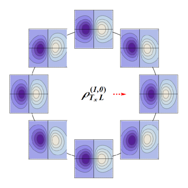
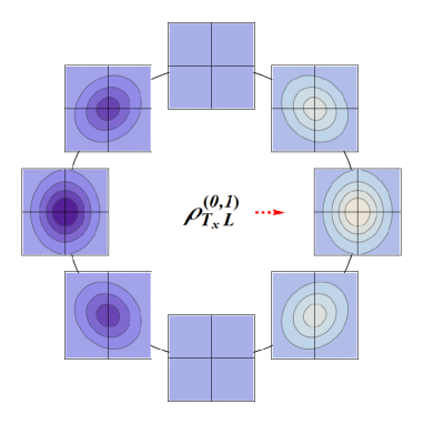
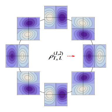
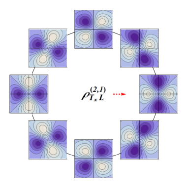
Figure 10: Naive $\mathsf{T}$-even (left) and $\mathsf{T}$-odd (right) contributions to the transverse phase-space distribution $\rho_{TL}$ for the target polarization $\vec{S}_{T}=\vec{e}_{x}$ (red dashed arrow). See text for more details.

The corresponding basic multipoles are

$$S^{i}_{T}S^{q}_{L}\,B^{(1,0)}_{T^{i}L}(\hat{k}_{T},\hat{b}_{T};\hat{P},\eta) =S^{i}_{T}S^{q}_{L}D^{i}_{k}M_{b}=S^{q}_{L}(\boldsymbol{S}_{T}\cdot\hat{k}_{T}),$$ (65)

$$S^{i}_{T}S^{q}_{L}\,B^{(1,2)}_{T^{i}L}(\hat{k}_{T},\hat{b}_{T};\hat{P},\eta) =S^{i}_{T}S^{q}_{L}D^{j}_{k}Q^{ij}_{b}=S^{q}_{L}\!\left[(\boldsymbol{S}_{T}\cdot\hat{b}_{T})\,(\hat{b}_{T}\cdot\hat{k}_{T})-\tfrac{1}{2}\,(\boldsymbol{S}_{T}\cdot\hat{k}_{T})\right],$$ (66)

$$S^{i}_{T}S^{q}_{L}\,B^{(0,1)}_{T^{i}L}(\hat{k}_{T},\hat{b}_{T};\hat{P},\eta) =\eta\,S^{i}_{T}S^{q}_{L}M_{k}D^{i}_{b}=\eta\,S^{q}_{L}(\boldsymbol{S}_{T}\cdot\hat{b}_{T}),$$ (67)

$$S^{i}_{T}S^{q}_{L}\,B^{(2,1)}_{T^{i}L}(\hat{k}_{T},\hat{b}_{T};\hat{P},\eta) =\eta\,S^{i}_{T}S^{q}_{L}Q^{ij}_{k}D^{j}_{b}=\eta\,S^{q}_{L}\!\left[(\boldsymbol{S}_{T}\cdot\hat{k}_{T})\,(\hat{k}_{T}\cdot\hat{b}_{T})-\tfrac{1}{2}\,(\boldsymbol{S}_{T}\cdot\hat{b}_{T})\right].$$ (68)

The contribution $\rho^{(1,0)}_{T^{i}L}$ is the only one surviving the integration over $\boldsymbol{b}_{T}$ and is then naturally related to the worm-gear TMD $g_{1T}$ Diehl:2005jf ; Lorce:2011dv . The dipole in $\boldsymbol{k}_{T}$-space indicates the presence of a net transverse flow parallel to the quark transverse polarization. This transverse flow is once again due to the light-front imaging, associated with the fact that the light-front densities are defined in terms of the $j^{+}=\tfrac{1}{\sqrt{2}}(j^{0}+j^{3})$ component of the current instead of the $j^{0}$ component. As we will soon see, it turns out that the transverse flow finds its physical origin in the correlation between the transverse component of quark OAM and the longitudinal spin-orbit coupling $\langle(\boldsymbol{S}_{T}\cdot\boldsymbol{\ell}^{q}_{T})S^{q}_{L}\ell^{q}_{L}\rangle$.

The contribution $\rho^{(1,2)}_{T^{i}L}$ corresponds to a completely new information which is not accessible via GPDs or TMDs at leading twist. Combined with $\rho^{(1,0)}_{T^{i}L}$, it tells us how the quark distribution is affected by the two transverse-longitudinal worm-gear correlations, say $\langle S_{x}\ell^{q}_{x}S^{q}_{L}\ell^{q}_{L}\rangle$ and $\langle S_{y}\ell^{q}_{y}S^{q}_{L}\ell^{q}_{L}\rangle$. Following the same arguments as in Sec. V.2.3, with $S_{L}\boldsymbol{S}_{T}^{q}$ replaced by $\boldsymbol{S}_{T}S^{q}_{L}$, we can relate the two coefficient functions $C^{(1,0)}_{T^{i}L}$ and $C^{(1,2)}_{T^{i}L}$ to the strength of the two transverse-longitudinal worm-gear correlations $\langle S_{x}\ell^{q}_{x}S^{q}_{L}\ell^{q}_{L}\rangle$ and $\langle S_{y}\ell^{q}_{y}S^{q}_{L}\ell^{q}_{L}\rangle$.

Similarly, the contribution $\rho^{(0,1)}_{T^{i}L}$ is the only one surviving the integration over $\boldsymbol{k}_{T}$. It cannot however be related to the GPD $\tilde{E}$ Diehl:2005jf ; Lorce:2011dv ; Pasquini:2007xz since the latter is $\eta$-independent. Once again, the dipole in $\boldsymbol{b}_{T}$-space indicates the presence of a spatial separation between quarks with opposite correlations. This is likely another effect due to the light-front imaging.

The contribution $\rho^{(2,1)}_{T^{i}L}$ corresponds to a completely new information which is not accessible via GPDs or TMDs at leading twist. Combined with $\rho^{(0,1)}_{T^{i}L}$, it tells us how the initial- and final-state interactions depend on the two transverse-longitudinal worm-gear correlations, say $\langle S_{x}\ell^{q}_{x}S^{q}_{L}\ell^{q}_{L}\rangle$ and $\langle S_{y}\ell^{q}_{y}S^{q}_{L}\ell^{q}_{L}\rangle$.

Following once again the same arguments as in Sec. V.2.3, with $S_{L}\boldsymbol{S}_{T}^{q}$ replaced by $\boldsymbol{S}_{T}S^{q}_{L}$, we can relate the two coefficient functions $C^{(0,1)}_{T^{i}L}$ and $C^{(2,1)}_{T^{i}L}$ to the strength of the $\langle S_{x}\ell^{q}_{x}S^{q}_{L}\ell^{q}_{L}\rangle$- and $\langle S_{y}\ell^{q}_{y}S^{q}_{L}\ell^{q}_{L}\rangle$-dependent parts of the force felt by the quark due to initial- and final-state interactions. In other words, the contributions $\rho^{(0,1)}_{T^{i}L}$ and $\rho^{(2,1)}_{T^{i}L}$ describe the difference of radial flows between quarks with opposite $\langle S_{x}\ell^{q}_{x}S^{q}_{L}\ell^{q}_{L}\rangle$ or $\langle S_{y}\ell^{q}_{y}S^{q}_{L}\ell^{q}_{L}\rangle$ correlations.

V.3.3 Transversely polarized quark

The contribution $\rho_{T^{i}T^{j}}$ describes how the quark distribution is affected by the correlation between the quark and target transverse polarizations. Focusing on the naive $\mathsf{T}$-even sector, we find four phase-space distributions

$$\rho^{e}_{T^{i}T^{j}}=\rho^{(0,0)}_{T^{i}T^{j}}+\rho^{(0,2)}_{T^{i}T^{j}}+\rho^{(2,0)}_{T^{i}T^{j}}+\rho^{(2,2)}_{T^{i}T^{j}},$$ (69)

which are represented in Fig. 11 for the target polarization $\vec{S}_{T}=\vec{e}_{x}$ and for the two quark polarizations $\vec{S}^{q}_{T}=\vec{e}_{x,y}$.

             

             

             

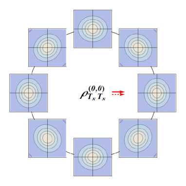
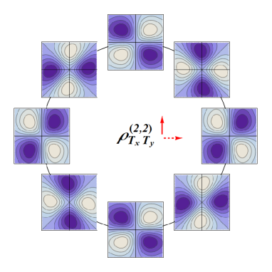
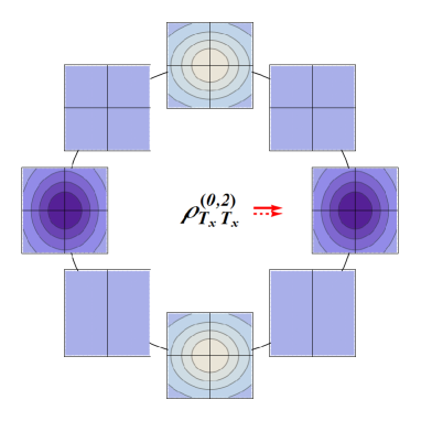
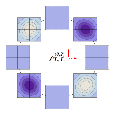
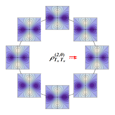
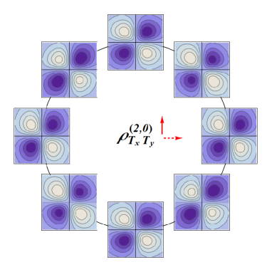
Figure 11: Naive $\mathsf{T}$-even contributions to the transverse phase-space distribution $\rho_{TT}$ for the target polarization $\vec{S}_{T}=\vec{e}_{x}$ (red dashed arrow) and for the two quark polarizations (red solid arrow) $\vec{S}^{q}_{T}=\vec{e}_{x}$ (left) and $\vec{S}^{q}_{T}=\vec{e}_{y}$ (right). See text for more details.

The corresponding basic multipoles are

$$S^{i}_{T}S^{qj}_{T}\,B^{(0,0)}_{T^{i}T^{j}}(\hat{k}_{T},\hat{b}_{T};\hat{P},\eta) =S^{i}_{T}S^{qi}_{L}M_{k}M_{b}=(\boldsymbol{S}_{T}\cdot\boldsymbol{S}^{q}_{T}),$$ (70)

$$S^{i}_{T}S^{qj}_{T}\,B^{(0,2)}_{T^{i}T^{j}}(\hat{k}_{T},\hat{b}_{T};\hat{P},\eta) =S^{i}_{T}S^{qj}_{T}M_{k}Q^{ij}_{b}=(\boldsymbol{S}_{T}\cdot\hat{b}_{T})\,(\hat{b}_{T}\cdot\boldsymbol{S}^{q}_{T})-\tfrac{1}{2}\,(\boldsymbol{S}_{T}\cdot\boldsymbol{S}^{q}_{T}),$$ (71)

$$S^{i}_{T}S^{qj}_{T}\,B^{(2,0)}_{T^{i}T^{j}}(\hat{k}_{T},\hat{b}_{T};\hat{P},\eta) =S^{i}_{T}S^{qj}_{T}Q^{ij}_{k}M_{b}=(\boldsymbol{S}_{T}\cdot\hat{k}_{T})\,(\hat{k}_{T}\cdot\boldsymbol{S}^{q}_{T})-\tfrac{1}{2}\,(\boldsymbol{S}_{T}\cdot\boldsymbol{S}^{q}_{T}),$$ (72)

$$S^{i}_{T}S^{qj}_{T}\,B^{(2,2)}_{T^{i}T^{j}}(\hat{k}_{T},\hat{b}_{T};\hat{P},\eta) =-S^{i}_{T}S^{qj}_{T}\epsilon^{ij}_{T}\epsilon^{mn}_{T}Q^{lm}_{k}Q^{ln}_{b}=(\boldsymbol{S}_{T}\times\boldsymbol{S}^{q}_{T})_{L}\,(\hat{b}_{T}\times\hat{k}_{T})_{L}\,(\hat{k}_{T}\cdot\hat{b}_{T}).$$ (73)

The contribution $\rho^{(0,0)}_{T^{i}T^{j}}$ is the only one surviving both integrations over $\boldsymbol{b}_{T}$ and $\boldsymbol{k}_{T}$, and is then naturally related to both the transversity GPD combination $H_{T}+\tfrac{\boldsymbol{\Delta}^{2}_{T}}{4M^{2}}\,\tilde{H}_{T}$ and the transversity TMD $h_{1}$ Diehl:2005jf ; Lorce:2011dv . Contrary to its $\boldsymbol{k}_{T}$- and $\boldsymbol{b}_{T}$-integrated versions, $\rho^{(0,0)}_{T^{i}T^{j}}$ is not circularly symmetric. The reason is that $\rho^{(0,0)}_{T^{i}T^{j}}$ also contains information about the correlation between $\boldsymbol{k}_{T}$ and $\boldsymbol{b}_{T}$, which is lost under integration over one of the transverse variables Lorce:2011kd .
Following the same arguments as in Sec. V.1.1 for $\rho_{UU}^{(0,0)}$, with now the corresponding expressions multiplied by $\boldsymbol{S}_{T}\cdot\boldsymbol{S}^{q}_{T}$, we can relate the coefficient function $C^{(0,0)}_{T^{i}T^{j}}$ to the strength of the correlation between the transverse component of quark and target polarizations $\langle\boldsymbol{S}_{T}\cdot\boldsymbol{S}^{q}_{T}\rangle$.

The contribution $\rho^{(0,2)}_{T^{i}T^{j}}$ is the only other contribution surviving integration over $\boldsymbol{k}_{T}$ and is then naturally related to the the GPD $\tilde{H}_{T}$ Diehl:2005jf ; Lorce:2011dv ; Pasquini:2007xz . Similarly, the contribution $\rho^{(2,0)}_{T^{i}T^{j}}$ is the only other contribution surviving integration over $\boldsymbol{b}_{T}$ and is then naturally related to the the pretzelosity TMD $h^{\perp}_{1T}$ Diehl:2005jf ; Miller:2007ae ; She:2009jq ; Avakian:2010br ; Lorce:2011kn . Combined with $\rho^{(0,0)}_{T^{i}T^{j}}$, these two contributions tell us how the quark distribution is affected by the two transverse spin-spin correlations, say $\langle S_{x}S^{q}_{x}\rangle$ and $\langle S_{y}S^{q}_{y}\rangle$. Indeed, let us consider the projection of a 3-dimensional $\langle(\vec{S}_{T}\cdot\vec{n}_{T})(\vec{S}^{q}_{T}\cdot\vec{n}_{T})\rangle$ correlation onto the transverse position space. For $\vec{n}_{T}=\vec{b}_{T}$ and $\vec{n}_{T}=(\vec{b}_{T}\times\hat{P})$, we respectively find

$$\int\mathrm{d}b_{L}\,(\vec{S}_{T}\cdot\vec{b}_{T})\,(\vec{S}^{q}_{T}\cdot\vec{b}_{T}) \sim(\boldsymbol{S}_{T}\cdot\hat{b}_{T})\,(\boldsymbol{S}^{q}_{T}\cdot\hat{b}_{T}),$$ (74)

$$\int\mathrm{d}b_{L}\,[\vec{S}_{T}\cdot(\vec{b}_{T}\times\hat{P})]\,[\vec{S}^{q}_{T}\cdot(\vec{b}_{T}\times\hat{P})] \sim(\boldsymbol{S}_{T}\times\hat{b}_{T})_{L}\,(\boldsymbol{S}^{q}_{T}\times\hat{b}_{T})_{L},$$ (75)

and similarly for $\vec{n}_{T}=\vec{k}_{T}$ and $\vec{n}_{T}=(\vec{k}_{T}\times\hat{P})$. Now, noting that for any unit transverse vector $\hat{n}_{T}$

$$(\boldsymbol{S}_{T}\cdot\hat{n}_{T})\,(\boldsymbol{S}^{q}_{T}\cdot\hat{n}_{T})+(\boldsymbol{S}_{T}\times\hat{n}_{T})_{L}\,(\boldsymbol{S}^{q}_{T}\times\hat{n}_{T})_{L}=(\boldsymbol{S}_{T}\cdot\boldsymbol{S}^{q}_{T})$$ (76)

and comparing with the basic multipoles (70), (71) and (72), we can see that the three coefficient functions $C^{(0,0)}_{T^{i}T^{j}}$, $C^{(0,2)}_{T^{i}T^{j}}$ and $C^{(2,0)}_{T^{i}T^{j}}$ are related to the strength of the two transverse spin-spin correlations $\langle S_{x}S^{q}_{x}\rangle$ and $\langle S_{y}S^{q}_{y}\rangle$.

It may seem weird that we need three contributions to determine two transverse spin-spin correlations. The reason is that the two contributions $\rho^{(0,2)}_{T^{i}T^{j}}$ and $\rho^{(2,0)}_{T^{i}T^{j}}$ also contain information about another type of correlation. Combined with $\rho^{(2,2)}_{T^{i}T^{j}}$, which corresponds to a completely new information not accessible via GPDs or TMDs at leading twist, they also tell us how the quark distribution is affected by the two transverse-transverse worm-gear correlations, say $\langle S_{x}\ell^{q}_{x}S^{q}_{y}\ell^{q}_{y}\rangle$ and $\langle S_{y}\ell^{q}_{y}S^{q}_{x}\ell^{q}_{x}\rangle$. Indeed, let us consider the projection of a 3-dimensional $\langle(\vec{S}_{T}\cdot\vec{n}_{T})(\vec{\ell}^{q}_{T}\cdot\vec{n}_{T})[\vec{S}^{q}_{T}\cdot(\vec{n}_{T}\times\hat{P})][\vec{\ell}^{q}_{T}\cdot(\vec{n}_{T}\times\hat{P})]\rangle$ correlation onto the transverse position space. For $\vec{n}_{T}=\vec{b}_{T}$ and $\vec{n}_{T}=(\vec{b}_{T}\times\hat{P})$, we respectively find

$$\int\mathrm{d}b_{L}\,(\vec{S}_{T}\cdot\vec{b}_{T})\,[(\vec{b}\times\vec{k})_{T}\cdot\vec{b}_{T}]\,[\vec{S}^{q}_{T}\cdot(\vec{b}_{T}\times\hat{P})]\,[(\vec{b}\times\vec{k})_{T}\cdot(\vec{b}_{T}\times\hat{P})] \sim(\boldsymbol{S}_{T}\cdot\hat{b}_{T})\,(\boldsymbol{S}^{q}_{T}\times\hat{b}_{T})_{L}\,(\hat{b}_{T}\times\hat{k}_{T})_{L}\,(\hat{k}_{T}\cdot\hat{b}_{T}),$$ (77)

$$\int\mathrm{d}b_{L}\,[\vec{S}_{T}\cdot(\vec{b}_{T}\times\hat{P})]\,[(\vec{b}\times\vec{k})_{T}\cdot(\vec{b}_{T}\times\hat{P})]\,(\vec{S}^{q}_{T}\cdot\vec{b}_{T})\,[(\vec{b}\times\vec{k})_{T}\cdot\vec{b}_{T})] \sim(\boldsymbol{S}_{T}\times\hat{b}_{T})_{L}\,(\boldsymbol{S}^{q}_{T}\cdot\hat{b}_{T})\,(\hat{b}_{T}\times\hat{k}_{T})_{L}\,(\hat{k}_{T}\cdot\hat{b}_{T}),$$ (78)

and similarly for $\vec{n}_{T}=\vec{k}_{T}$ and $\vec{n}_{T}=(\vec{k}_{T}\times\hat{P})$. Now, noting that for any unit transverse vector $\hat{n}_{T}$

$$(\boldsymbol{S}_{T}\times\hat{n}_{T})_{L}\,(\boldsymbol{S}^{q}_{T}\cdot\hat{n}_{T})- (\boldsymbol{S}_{T}\cdot\hat{n}_{T})\,(\boldsymbol{S}^{q}_{T}\times\hat{n}_{T})_{L}=(\boldsymbol{S}_{T}\times\boldsymbol{S}^{q}_{T})_{L},$$ (79)

$$[(\boldsymbol{S}_{T}\times\hat{n}_{T})_{L}\,(\boldsymbol{S}^{q}_{T}\cdot\hat{n}_{T})+ (\boldsymbol{S}_{T}\cdot\hat{n}_{T})\,(\boldsymbol{S}^{q}_{T}\times\hat{n}_{T})_{L}]\,(\hat{b}_{T}\times\hat{k}_{T})_{L}\,(\hat{k}_{T}\cdot\hat{b}_{T})$$

$$=[(\hat{k}_{T}\cdot\hat{n}_{T})^{2}-(\hat{k}_{T}\times\hat{n}_{T})^{2}_{L}]\,[(\boldsymbol{S}_{T}\cdot\hat{b}_{T})\,(\hat{b}_{T}\cdot\boldsymbol{S}^{q}_{T})-\tfrac{1}{2}\,(\boldsymbol{S}_{T}\cdot\boldsymbol{S}^{q}_{T})]$$

$$- [(\hat{b}_{T}\cdot\hat{n}_{T})^{2}-(\hat{b}_{T}\times\hat{n}_{T})^{2}_{L}]\,[(\boldsymbol{S}_{T}\cdot\hat{k}_{T})\,(\hat{k}_{T}\cdot\boldsymbol{S}^{q}_{T})-\tfrac{1}{2}\,(\boldsymbol{S}_{T}\cdot\boldsymbol{S}^{q}_{T})],$$ (80)

and comparing with the basic multipoles (71), (72) and (73), we can see that the three coefficient functions $C^{(0,2)}_{T^{i}T^{j}}$, $C^{(2,0)}_{T^{i}T^{j}}$ and $C^{(2,2)}_{T^{i}T^{j}}$ are related to the strength of the two transverse-transverse worm-gear correlations $\langle S_{x}\ell^{q}_{x}S^{q}_{y}\ell^{q}_{y}\rangle$ and $\langle S_{y}\ell^{q}_{y}S^{q}_{x}\ell^{q}_{x}\rangle$.

Focusing now on the naive $\mathsf{T}$-odd sector, we also find four phase-space distributions

$$\rho^{o}_{T^{i}T^{j}}=\rho^{(1,1)}_{T^{i}T^{j}}+\rho^{(1,3)}_{T^{i}T^{j}}+\rho^{(3,1)}_{T^{i}T^{j}}+\rho^{(1,1)^{\prime}}_{T^{i}T^{j}},$$ (81)

which are represented in Fig. 12 for the target polarization $\vec{S}_{T}=\vec{e}_{x}$ and for the two quark polarizations $\vec{S}^{q}_{T}=\vec{e}_{x,y}$.

             

             

             

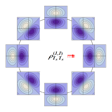
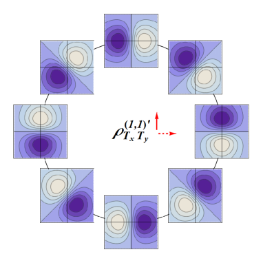
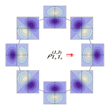
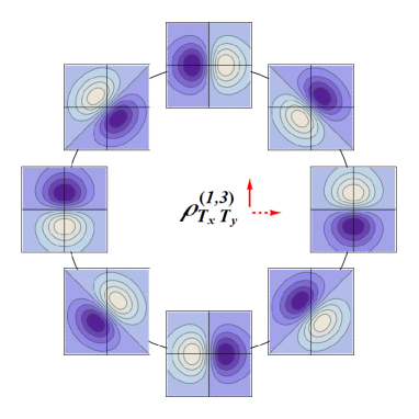
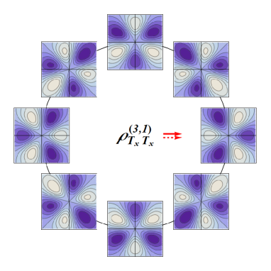
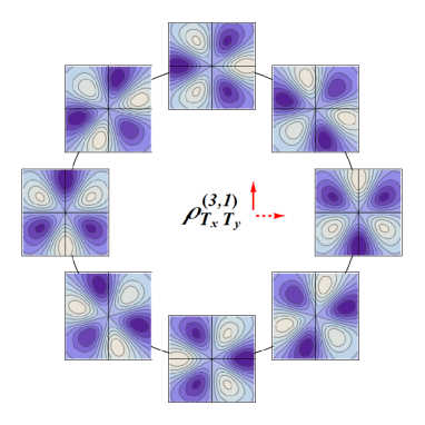
Figure 12: Naive $\mathsf{T}$-odd contributions to the transverse phase-space distribution $\rho_{TT}$ for the target polarization $\vec{S}_{T}=\vec{e}_{x}$ (red dashed arrow) and for the two quark polarizations (red solid arrow) $\vec{S}^{q}_{T}=\vec{e}_{x}$ (left) and $\vec{S}^{q}_{T}=\vec{e}_{y}$ (right). See text for more details.

The corresponding basic multipoles are

$$S^{i}_{T}S^{qj}_{T}\,B^{(1,1)}_{T^{i}T^{j}}(\hat{k}_{T},\hat{b}_{T};\hat{P},\eta) =S^{i}_{T}S^{qi}_{L}D^{j}_{k}D^{j}_{b}=(\boldsymbol{S}_{T}\cdot\boldsymbol{S}^{q}_{T})\,(\hat{k}_{T}\cdot\hat{b}_{T}),$$ (82)

$$S^{i}_{T}S^{qj}_{T}\,B^{(1,3)}_{T^{i}T^{j}}(\hat{k}_{T},\hat{b}_{T};\hat{P},\eta) =S^{i}_{T}S^{qj}_{T}D^{l}_{k}O^{ijl}_{b}$$

$$=(\boldsymbol{S}_{T}\cdot\hat{b}_{T})\,(\boldsymbol{S}^{q}_{T}\cdot\hat{b}_{T}) \,(\hat{k}_{T}\cdot\hat{b}_{T})-\tfrac{1}{4}\,[(\boldsymbol{S}_{T}\cdot\boldsymbol{S}^{q}_{T})\,(\hat{k}_{T}\cdot\hat{b}_{T})+(\boldsymbol{S}_{T}\cdot\hat{b}_{T})\,(\boldsymbol{S}^{q}_{T}\cdot\hat{k}_{T})+(\boldsymbol{S}_{T}\cdot\hat{k}_{T})\,(\boldsymbol{S}^{q}_{T}\cdot\hat{b}_{T})],$$ (83)

$$S^{i}_{T}S^{qj}_{T}\,B^{(3,1)}_{T^{i}T^{j}}(\hat{k}_{T},\hat{b}_{T};\hat{P},\eta) =S^{i}_{T}S^{qj}_{T}O^{ijl}_{k}D^{l}_{b}$$

$$=(\boldsymbol{S}_{T}\cdot\hat{k}_{T})\,(\boldsymbol{S}^{q}_{T}\cdot\hat{k}_{T}) \,(\hat{k}_{T}\cdot\hat{b}_{T})-\tfrac{1}{4}\,[(\boldsymbol{S}_{T}\cdot\boldsymbol{S}^{q}_{T})\,(\hat{k}_{T}\cdot\hat{b}_{T})+(\boldsymbol{S}_{T}\cdot\hat{b}_{T})\,(\boldsymbol{S}^{q}_{T}\cdot\hat{k}_{T})+(\boldsymbol{S}_{T}\cdot\hat{k}_{T})\,(\boldsymbol{S}^{q}_{T}\cdot\hat{b}_{T})],$$ (84)

$$S^{i}_{T}S^{qj}_{T}\,B^{(1,1)^{\prime}}_{T^{i}T^{j}}(\hat{k}_{T},\hat{b}_{T};\hat{P},\eta) =-S^{i}_{T}S^{qj}_{T}\epsilon^{ij}_{T}\epsilon^{lm}_{T}D^{l}_{k}D^{m}_{b}=(\boldsymbol{S}_{T}\times\boldsymbol{S}^{q}_{T})_{L}\,(\hat{b}_{T}\times\hat{k}_{T})_{L}.$$ (85)

None of these survive integration over $\boldsymbol{k}_{T}$ or $\boldsymbol{b}_{T}$. They therefore represent completely new information which is not accessible via GPDs or TMDs at leading twist.

Following the same arguments as in Sec. V.1.1 for $\rho_{UU}^{(1,1)}$, with now the corresponding expressions multiplied by $\boldsymbol{S}_{T}\cdot\boldsymbol{S}^{q}_{T}$, we can relate the coefficient function $C^{(1,1)}_{T^{i}T^{j}}$ to the strength of the correlation between the transverse component of quark and target polarizations $\langle\boldsymbol{S}_{T}\cdot\boldsymbol{S}^{q}_{T}\rangle$. Combining $\rho^{(1,1)}_{T^{i}T^{j}}$ with $\rho^{(1,3)}_{T^{i}T^{j}}$ and $\rho^{(3,1)}_{T^{i}T^{j}}$ tells us how the initial- and final-state interactions depend separately on the two transverse spin-spin correlations, say $\langle S_{x}S^{q}_{x}\rangle$ and $\langle S_{y}S^{q}_{y}\rangle$. Indeed, let us consider the projection of a 3-dimensional radial flow $(\vec{S}_{T}\cdot\vec{n}_{T})\,(\vec{S}^{q}_{T}\cdot\vec{n}_{T})\,(\vec{k}\cdot\vec{b})$ onto the transverse position space. For $\vec{n}_{T}=\vec{b}_{T}$ and $\vec{n}_{T}=(\vec{b}_{T}\times\hat{P})$, we respectively find

$$\int\mathrm{d}b_{L}\,(\vec{S}_{T}\cdot\vec{b}_{T})\,(\vec{S}^{q}_{T}\cdot\vec{b}_{T})\,(\vec{k}\cdot\vec{b}) \sim(\boldsymbol{S}_{T}\cdot\hat{b}_{T})\,(\boldsymbol{S}^{q}_{T}\cdot\hat{b}_{T})\,(\hat{k}_{T}\cdot\hat{b}_{T}),$$ (86)

$$\int\mathrm{d}b_{L}\,[\vec{S}_{T}\cdot(\vec{b}_{T}\times\hat{P})]\,[\vec{S}^{q}_{T}\cdot(\vec{b}_{T}\times\hat{P})]\,(\vec{k}\cdot\vec{b}) \sim(\boldsymbol{S}_{T}\times\hat{b}_{T})_{L}\,(\boldsymbol{S}^{q}_{T}\times\hat{b}_{T})_{L}\,(\hat{k}_{T}\cdot\hat{b}_{T}),$$ (87)

and similarly for $\vec{n}_{T}=\vec{k}_{T}$ and $\vec{n}_{T}=(\vec{k}_{T}\times\hat{P})$. Now, noting that for any unit transverse vectors $\hat{n}_{T}$ and $\hat{n}^{\prime}_{T}$

$$(\boldsymbol{S}_{T}\cdot\hat{n}_{T})\,(\boldsymbol{S}^{q}_{T}\cdot\hat{n}_{T})+(\boldsymbol{S}_{T}\times\hat{n}_{T})_{L}\,(\boldsymbol{S}^{q}_{T}\times\hat{n}_{T})_{L} =(\boldsymbol{S}_{T}\cdot\boldsymbol{S}^{q}_{T}),$$ (88)

$$(\boldsymbol{S}_{T}\cdot\hat{n}_{T})\,(\boldsymbol{S}^{q}_{T}\cdot\hat{n}_{T})(\hat{n}_{T}\cdot\hat{n}^{\prime}_{T})+(\boldsymbol{S}_{T}\cdot\hat{n}^{\prime}_{T})\,(\boldsymbol{S}^{q}_{T}\cdot\hat{n}^{\prime}_{T})(\hat{n}^{\prime}_{T}\cdot\hat{n}_{T})$$

$$=[(\boldsymbol{S}_{T}\cdot\hat{n}_{T})\,(\boldsymbol{S}^{q}_{T}\cdot\hat{n}^{\prime}_{T})+(\boldsymbol{S}_{T}\cdot\hat{n}^{\prime}_{T})\,(\boldsymbol{S}^{q}_{T}\cdot\hat{n}_{T})]\,(\hat{n}_{T}\cdot\hat{n}^{\prime}_{T})^{2} +[(\boldsymbol{S}_{T}\cdot\boldsymbol{S}^{q}_{T})(\hat{n}_{T}\cdot\hat{n}^{\prime}_{T})]\,(\hat{n}_{T}\times\hat{n}^{\prime}_{T})^{2}_{L},$$ (89)

and comparing with the basic multipoles (82), (83) and (84), we can see that the three coefficient functions $C^{(1,1)}_{T^{i}T^{j}}$, $C^{(1,3)}_{T^{i}T^{j}}$ and $C^{(3,1)}_{T^{i}T^{j}}$ are related to the strength of the $\langle S_{x}S^{q}_{x}\rangle$- and $\langle S_{y}S^{q}_{y}\rangle$-dependent parts of the force felt by the quark due to initial- and final-state interactions. In other words, the contributions $\rho^{(1,1)}_{T^{i}T^{j}}$, $\rho^{(1,3)}_{T^{i}T^{j}}$ and $\rho^{(3,1)}_{T^{i}T^{j}}$ describe the difference of radial flows between quarks with opposite $\langle S_{x}S^{q}_{x}\rangle$ or $\langle S_{y}S^{q}_{y}\rangle$ correlations.

Like in the naive $\mathsf{T}$-even sector, it may seem weird that we need three contributions to determine the dependence of initial- and final-state interactions on two transverse spin-spin correlations. The reason is that the two contributions $\rho^{(1,3)}_{T^{i}T^{j}}$ and $\rho^{(3,1)}_{T^{i}T^{j}}$ also contain information about another type of dependence. Combined with $\rho^{(1,1)^{\prime}}_{T^{i}T^{j}}$, they also tell us how the initial- and final-state interactions depend separately on the two transverse-transverse worm-gear correlations, say $\langle S_{x}\ell^{q}_{x}S^{q}_{y}\ell^{q}_{y}\rangle$ and $\langle S_{y}\ell^{q}_{y}S^{q}_{x}\ell^{q}_{x}\rangle$. Indeed, let us consider the projection of a 3-dimensional spiral worm-gear flow $(\vec{S}_{T}\cdot\vec{n}_{T})(\vec{\ell}^{q}_{T}\cdot\vec{n}_{T})[\vec{S}^{q}_{T}\cdot(\vec{n}_{T}\times\hat{P})][\vec{\ell}^{q}_{T}\cdot(\vec{n}_{T}\times\hat{P})](\vec{k}\cdot\vec{b})$ onto the transverse position space. For $\vec{n}_{T}=\vec{b}_{T}$ and $\vec{n}_{T}=(\vec{b}_{T}\times\hat{P})$, we respectively find

$$\int\mathrm{d}b_{L}\,(\vec{S}_{T}\cdot\vec{b}_{T})\,[(\vec{b}\times\vec{k})_{T}\cdot\vec{b}_{T}]\,[\vec{S}^{q}_{T}\cdot(\vec{b}_{T}\times\hat{P})]\,[(\vec{b}\times\vec{k})_{T}\cdot(\vec{b}_{T}\times\hat{P})]\,(\vec{k}\cdot\vec{b}) \sim(\boldsymbol{S}_{T}\cdot\hat{b}_{T})\,(\boldsymbol{S}^{q}_{T}\times\hat{b}_{T})_{L}\,(\hat{b}_{T}\times\hat{k}_{T})_{L},$$ (90)

$$\int\mathrm{d}b_{L}\,[\vec{S}_{T}\cdot(\vec{b}_{T}\times\hat{P})]\,[(\vec{b}\times\vec{k})_{T}\cdot(\vec{b}_{T}\times\hat{P})]\,(\vec{S}^{q}_{T}\cdot\vec{b}_{T})\,[(\vec{b}\times\vec{k})_{T}\cdot\vec{b}_{T}]\,(\vec{k}\cdot\vec{b}) \sim(\boldsymbol{S}_{T}\times\hat{b}_{T})_{L}\,(\boldsymbol{S}^{q}_{T}\cdot\hat{b}_{T})\,(\hat{b}_{T}\times\hat{k}_{T})_{L},$$ (91)

and similarly for $\vec{n}_{T}=\vec{k}_{T}$ and $\vec{n}_{T}=(\vec{k}_{T}\times\hat{P})$. Noting that for any unit transverse vectors $\hat{n}_{T}$ and $\hat{n}^{\prime}_{T}$

$$(\boldsymbol{S}_{T}\times\hat{n}_{T})_{L}\,(\boldsymbol{S}^{q}_{T}\cdot\hat{n}_{T})- (\boldsymbol{S}_{T}\cdot\hat{n}_{T})\,(\boldsymbol{S}^{q}_{T}\times\hat{n}_{T})_{L}=(\boldsymbol{S}_{T}\times\boldsymbol{S}^{q}_{T})_{L},$$ (92)

$$4(\boldsymbol{S}_{T}\cdot\hat{n}_{T})\,(\boldsymbol{S}^{q}_{T}\cdot\hat{n}_{T})\,(\hat{n}_{T}\cdot\hat{n}^{\prime}_{T})- [(\boldsymbol{S}_{T}\cdot\boldsymbol{S}^{q}_{T})\,(\hat{n}_{T}\cdot\hat{n}^{\prime}_{T})+(\boldsymbol{S}_{T}\cdot\hat{n}_{T})\,(\boldsymbol{S}^{q}_{T}\cdot\hat{n}^{\prime}_{T})+(\boldsymbol{S}_{T}\cdot\hat{n}^{\prime}_{T})\,(\boldsymbol{S}^{q}_{T}\cdot\hat{n}_{T})]$$

$$=[(\boldsymbol{S}_{T}\cdot\hat{n}_{T})\,(\boldsymbol{S}^{q}_{T}\cdot\hat{n}_{T})-(\boldsymbol{S}_{T}\times\hat{n}_{T})_{L}\,(\boldsymbol{S}^{q}_{T}\times\hat{n}_{T})_{L}]\,(\hat{n}_{T}\cdot\hat{n}^{\prime}_{T})$$

$$+ [(\boldsymbol{S}_{T}\cdot\hat{n}_{T})\,(\boldsymbol{S}^{q}_{T}\times\hat{n}_{T})_{L}+(\boldsymbol{S}_{T}\times\hat{n}_{T})_{L}\,(\boldsymbol{S}^{q}_{T}\cdot\hat{n}_{T})]\,(\hat{n}_{T}\times\hat{n}^{\prime}_{T})_{L},$$ (93)

and comparing with the basic multipoles (83), (84) and (85), we can see that the three coefficient functions $C^{(1,3)}_{T^{i}T^{j}}$, $C^{(3,1)}_{T^{i}T^{j}}$ and $C^{(1,1)^{\prime}}_{T^{i}T^{j}}$ are related to the strength of the $\langle S_{x}\ell^{q}_{x}S^{q}_{y}\ell^{q}_{y}\rangle$- and $\langle S_{y}\ell^{q}_{y}S^{q}_{x}\ell^{q}_{x}\rangle$-dependent parts of the force felt by the quark due to initial- and final-state interactions. In other words, the contributions $\rho^{(1,3)}_{T^{i}T^{j}}$, $\rho^{(3,1)}_{T^{i}T^{j}}$ and $\rho^{(1,1)^{\prime}}_{T^{i}T^{j}}$ describe the difference of radial flows between quarks with opposite $\langle S_{x}\ell^{q}_{x}S^{q}_{y}\ell^{q}_{y}\rangle$ or $\langle S_{y}\ell^{q}_{y}S^{q}_{x}\ell^{q}_{x}\rangle$ correlations.

VI Conclusions

We presented for the first time a systematic study of the complete set of the leading-twist quark Wigner distributions in the nucleon, introducing a multipole analysis in the transverse phase space. In this approach each distribution is represented as combination of basic multipoles structures multiplied by coefficient functions giving the corresponding strengths. The multipole structures are obtained for each configuration of the nucleon and target polarizations, taking into account the constraints from hermiticity, parity and time-reversal transformations, while the coefficient functions depend on $\mathsf{P}$- and $\mathsf{T}$-invariant hermitian variables only. There are several advantages in using this representation. First, it provides a clear interpretation of all the amplitudes in terms of the possible correlations between target and quark angular momenta in the transverse phase space. Second, it provides a convenient basis to make a direct connection with GPDs in impact-parameter space and TMD in transverse-momentum space after integration over the transverse-momentum and the transverse-position space, respectively. In order to emphasize these multipole structures, we also proposed a new graphical representation of the transverse phase-space distributions.

We presented results for both the naive $\mathsf{T}$-even and naive $\mathsf{T}$-odd contributions. The first ones describe the contributions to the intrinsic distribution of quarks inside the target, whereas the naive $\mathsf{T}$-odd contributions describe how initial- and final-state interactions modify this distribution. We have explicitly calculated the naive $\mathsf{T}-$even contributions adopting a light-front quark model, whereas the naive $\mathsf{T}$-odd contributions have been obtained by extracting the coefficient functions from the naive $\mathsf{T}$-even part and multiplying them by the appropriate basic multipoles. In this way, the global sign of the naive $\mathsf{T}$-odd contributions has been chosen arbitrarily. Only a proper calculation taking into account the dynamics of the initial- and/or final-state interactions can determine the global signs. However, these global signs are not important for the purpose of the present paper since we wanted to emphasize the general features related to the multipole structure of the distribution, and to identify the physical (angular) correlation encoded in each distribution.

References

- (1) E. P. Wigner, Phys. Rev. 40, 749 (1932).
- (2) N. L. Balazs and B. K. Jennings, Phys. Rept. 104, 347 (1984).
- (3) M. Hillery, R. F. O’Connell, M. O. Scully and E. P. Wigner, Phys. Rept. 106, 121 (1984).
- (4) H.-W. Lee, Phys. Rept. 259, 147 (1995).
- (5) P. Carruthers and F. Zachariasen, Rev. Mod. Phys. 55, 245 (1983).
- (6) R. Hakim, Riv. Nuovo Cim. 1N6, 1 (1978). doi:10.1007/BF02724474
- (7) S. R. De Groot, W. A. Van Leeuwen and C. G. Van Weert, Amsterdam, Netherlands: North-holland ( 1980) 417p
- (8) H. T. Elze, M. Gyulassy and D. Vasak, Nucl. Phys. B 276, 706 (1986).
- (9) S. Ochs and U. W. Heinz, Annals Phys. 266, 351 (1998).
- (10) U. W. Heinz, Phys. Rev. Lett. 51, 351 (1983). doi:10.1103/PhysRevLett.51.351
- (11) U. W. Heinz, Annals Phys. 161, 48 (1985). doi:10.1016/0003-4916(85)90336-7
- (12) H. T. Elze, M. Gyulassy and D. Vasak, Phys. Lett. B 177, 402 (1986). doi:10.1016/0370-2693(86)90778-1
- (13) X. d. Ji, Phys. Rev. Lett. 91, 062001 (2003).
- (14) A. V. Belitsky, X. d. Ji and F. Yuan, Phys. Rev. D 69, 074014 (2004).
- (15) D. E. Soper, Phys. Rev. D 15, 1141 (1977).
- (16) M. Burkardt, Phys. Rev. D 62, 071503 (2000) [Erratum-ibid. D 66, 119903 (2002)].
- (17) M. Burkardt, Int. J. Mod. Phys. A 18, 173 (2003).
- (18) M. Burkardt, Phys. Rev. D 72, 094020 (2005).
- (19) C. Lorcé and B. Pasquini, Phys. Rev. D 84, 014015 (2011).
- (20) S. Meissner, A. Metz and M. Schlegel, JHEP 0908, 056 (2009).
- (21) C. Lorcé, B. Pasquini and M. Vanderhaeghen, JHEP 1105, 041 (2011).
- (22) C. Lorcé and B. Pasquini, JHEP 1309, 138 (2013).
- (23) Y. Hatta, Phys. Lett. B 708, 186 (2012).
- (24) C. Lorcé, B. Pasquini, X. Xiong and F. Yuan, Phys. Rev. D 85, 114006 (2012).
- (25) K. F. Liu and C. Lorcé, arXiv:1508.00911 [hep-ph].
- (26) A. D. Martin, M. G. Ryskin and T. Teubner, Phys. Rev. D 62, 014022 (2000).
- (27) V. A. Khoze, A. D. Martin and M. G. Ryskin, Eur. Phys. J. C 14, 525 (2000).
- (28) A. D. Martin and M. G. Ryskin, Phys. Rev. D 64, 094017 (2001).
- (29) M. G. Albrow et al. [FP420 R and D Collaboration], JINST 4, T10001 (2009).
- (30) A. D. Martin, M. G. Ryskin and V. A. Khoze, Acta Phys. Polon. B 40, 1841 (2009).
- (31) K. Kanazawa, C. Lorcé, A. Metz, B. Pasquini and M. Schlegel, Phys. Rev. D 90, 014028 (2014).
- (32) A. Mukherjee, S. Nair and V. K. Ojha, Phys. Rev. D 90, 014024 (2014).
- (33) T. Liu, arXiv:1406.7709 [hep-ph].
- (34) T. Liu and B. Q. Ma, Phys. Rev. D 91, 034019 (2015).
- (35) G. A. Miller, Phys. Rev. D 90, 113001 (2014).
- (36) A. Mukherjee, S. Nair and V. K. Ojha, Phys. Rev. D 91, 054018 (2015).
- (37) M. Burkardt and B. Pasquini, arXiv:1510.02567 [hep-ph].
- (38) X. Ji, Phys. Rev. Lett. 110, 262002 (2013).
- (39) C. Lorcé and B. Pasquini, Phys. Rev. D 84, 034039 (2011).
- (40) D. E. Soper, Phys. Rev. D 5, 1956 (1972).
- (41) C. E. Carlson and C. R. Ji, Phys. Rev. D 67, 116002 (2003).
- (42) S. J. Brodsky, S. Gardner and D. S. Hwang, Phys. Rev. D 73, 036007 (2006).
- (43) M. Diehl and P. Hagler, Eur. Phys. J. C 44, 87 (2005).
- (44) C. Lorcé, JHEP 1508, 045 (2015).
- (45) C. Lorcé, Phys. Lett. B 719, 185 (2013).
- (46) M.G. Echevarria et al., in preparation.
- (47) C. Lorcé, Phys. Lett. B 735, 344 (2014).
- (48) B. Pasquini and S. Boffi, Phys. Lett. B 653, 23 (2007).
- (49) C. Møller, Commun. Dublin Inst. Adv. Stud. A 5, 1 (1949).
- (50) C. Møller, The Theory of Relativity, 2nd ed., Oxford Univ. Press, Oxford, 1972, p. 176.
- (51) M. I. Dyakonov and V. I. Perel, Sov. Phys. JETP Lett. 13, 467 (1971).
- (52) M. I. Dyakonov and V. I. Perel, Phys. Lett. A 35, 459 (1971).
- (53) X. Ji, X. Xiong and F. Yuan, Phys. Rev. D 88, no. 1, 014041 (2013).
- (54) Y. Hatta and S. Yoshida, JHEP 1210, 080 (2012).
- (55) A. Bacchetta and M. Radici, Phys. Rev. Lett. 107, 212001 (2011).
- (56) G. A. Miller, Phys. Rev. C 76, 065209 (2007).
- (57) J. She, J. Zhu and B. Q. Ma, Phys. Rev. D 79, 054008 (2009).
- (58) H. Avakian, A. V. Efremov, P. Schweitzer and F. Yuan, Phys. Rev. D 81, 074035 (2010).
- (59) C. Lorcé and B. Pasquini, Phys. Lett. B 710, 486 (2012).