Improved variational approach to QCD in Coulomb gauge

Abstract

The variational approach to QCD in Coulomb gauge developed previously by the Tübingen group is improved by enlarging the space of quark trial vacuum wave functionals through a new Dirac structure in the quark-gluon coupling. Our ansatz for the quark vacuum wave functional ensures that all linear divergences cancel in the quark gap equation resulting from the minimization of the energy calculated to two-loop order. The logarithmic divergences are absorbed in a renormalized coupling which is adjusted to reproduce the phenomenological value of the quark condensate. We also unquench the gluon propagator and show that the unquenching effects are generally small and amount to a small reduction in the mid-momentum regime.

I Introduction

During the last two decades the infrared sector of QCD was intensively studied both on the lattice and in the continuum theory. Substantial insight into the two basic features of the QCD vacuum, confinement and spontaneous breaking of chiral symmetry (SBCS), has been gained although a rigorous understanding of these two phenomena is still lacking. Confinement is a property of the Yang–Mills sector. Indeed, the order parameter of confinement, the Wilson loop, is a purely gluonic observable, from which the static quark potential can be extracted. SBCS takes place in the quark sector: The quarks in the Dirac vacuum condense similar as the electrons in a superconductor, and the first microscopic explanations of the SBCS were based on superconductor types of effective models like the Nambu–Jona-Lasinio model Nambu and Jona-Lasinio (1961a, b); Ebert and Reinhardt (1986). Indeed, the order parameter of SBCS is the quark condensate. However, by the Banks–Casher relation Banks and Casher (1980) this order parameter is related to the level density near zero virtuality of the quarks in the fluctuating gluonic background. Consequently, SBCS is also caused indirectly by the gluons.

Extensive lattice studies have shown that confinement and SBCS are both caused by topologically non-trivial field configurations like center vortices and magnetic monopoles, see ref. Greensite (2011) for a review. Indeed, when center vortices or magnetic monopoles are removed by hand from the ensemble of gauge field configurations the area law of the Wilson loop and thus the confining part of the extracted quark potential is lost Del Debbio et al. (1998); Engelhardt et al. (2000). At the same time the level density of the quarks develops a gap near zero virtuality Gattnar et al. (2005) and, by the Banks–Casher relation, SBCS disappears. On the other hand, when one projects the ensemble of gauge field configurations on those containing center vortices, the short distance Coulomb part of the static quark potential disappears while the linearly rising confining part is preserved at all distances. At the same time the quark levels are squeezed in the region around zero virtuality Höllwieser et al. (2008).

A seemingly different confinement scenario was proposed by Gribov Gribov (1978) and further developed by Zwanziger Zwanziger (1998), in which confinement manifests itself in an infrared diverging ghost form factor. Extensive studies, both on the lattice and in the continuum, have shown that this picture is not realized in Landau gauge Cucchieri and Mendes (2007) (as originally assumed) but only in Coulomb gauge Feuchter and Reinhardt (2004a, b); Epple et al. (2007); Burgio et al. (2009). Though confinement is a gauge invariant phenomenon, it may manifest itself differently in different gauges. In Coulomb gauge not only an infrared diverging ghost form factor but also a linearly rising static quark potential (the so-called non-Abelian Coulomb potential) is obtained. The infrared slope of this potential is given by the so-called Coulomb string tension, which is an upper bound to the Wilson string tension Zwanziger (2003). The Gribov–Zwanziger picture was mainly established within the Hamiltonian approach to QCD in Coulomb gauge by means of variational calculations Feuchter and Reinhardt (2004a, b); Epple et al. (2007); Szczepaniak and Swanson (2001) and is also supported by lattice calculations Burgio et al. (2009); Greensite et al. (2004). Lattice and continuum studies have shown that the Gribov–Zwanziger confinement scenario is tightly related to the center vortex and magnetic monopole pictures of confinement: Center vortices and magnetic monopoles live on the so-called Gribov horizon Greensite et al. (2004), i.e. are field configurations for which the Faddeev–Popov determinant vanishes. When these center vortices are removed from the Yang–Mills ensemble, the ghost form factor becomes infrared finite and the non-Abelian Coulomb potential is no longer linearly rising but becomes infrared flat Greensite et al. (2004), i.e. the Coulomb string tension disappears. Recently, it was also shown that the Coulomb string tension is not related to the temporal Wilson string tension but to the spatial string tension Burgio et al. (2015). This also explains why the Coulomb string tension does not disappear above the deconfinement phase transition Vogt et al. (2014). Furthermore, within the Hamiltonian approach in Coulomb gauge it was shown that the inverse of the ghost form factor can be interpreted as the dielectric function of the Yang–Mills vacuum Reinhardt (2008). An infrared diverging ghost form factor then implies that the dielectric function vanishes in the infrared, which makes the Yang–Mills vacuum a perfect color dielectricum, i.e. a dual superconductor, which arises from the condensation of magnetic monopoles. In this sense the Gribov–Zwanziger picture is also related to the magnetic monopole picture of confinement.

Variational calculations within the Hamiltonian approach in Coulomb gauge were initiated in ref. Schütte (1985), where a Gaussian trial ansatz was used for the Yang–Mills vacuum wave functional. The same ansatz was used in ref. Szczepaniak and Swanson (2001) where also the first numerical calculations were carried out. The approach developed by the Tübingen group Feuchter and Reinhardt (2004a, b); Epple et al. (2007) differs from previous work in the choice of the trial wave functional and more importantly in the treatment of the Faddeev–Popov determinant as well as in the renormalization, see ref. Greensite et al. (2011) for more details. In fact, in previous work the Faddeev–Popov determinant was not (properly) included. However, it turns out that the Faddeev–Popov determinant is crucial for the infrared properties of the theory and for the Gribov–Zwanziger picture to be realized Feuchter and Reinhardt (2004a, b); Epple et al. (2007). Within our approach we have obtained a decent description of the infrared properties of QCD as, for example, an infrared diverging gluon energy Feuchter and Reinhardt (2004a, b); Epple et al. (2007) (which is a signal of gluon confinement and also supported by the lattice calculation Burgio et al. (2009)), a linearly rising non-Abelian Coulomb potential, an infrared finite running coupling constant Epple et al. (2007), a perimeter law for the ’t Hooft loop Reinhardt and Epple (2007) and an area law for the Wilson loop Pak and Reinhardt (2009). For a recent review, see ref. Reinhardt et al. (2015).

The advantage of the Hamiltonian approach in Coulomb gauge is that the gauge fixed Hamiltonian contains already a confining four-quark interaction, which depends on the fluctuating transversal gauge field by the so-called Coulomb kernel, see eqs. (11) and (12). If this kernel is replaced by its Yang–Mills vacuum expectation value a confining quark potential is obtained. Keeping from the gauge fixed QCD Hamiltonian only this confining two-body interaction and the free Dirac Hamiltonian of the quarks one obtains a confining quark model, which has been treated originally by Finger and Mandula within a variational approach using for the quark vacuum wave functional a BCS-type of ansatz Finger and Mandula (1982). From this model one finds indeed SBCS but the quark condensate turns out to be much too small compared to the phenomenological values when realistic values for the Coulomb string tension are used. The model was reconsidered in Adler and Davis (1984) where the renormalization was improved and also in ref. Le Yaouanc et al. (1984) and was extended to non-zero current quark masses in ref. Alkofer and Amundsen (1988). Similar studies of chiral symmetry breaking within quark models with confining two-body interactions were carried out in de A. Bicudo and Ribeiro (1990) and Szczepaniak and Krupinski (2002).

The variational approach to Yang–Mills theory developed in ref. Feuchter and Reinhardt (2004a, b) was extended in refs. Pak and Reinhardt (2012, 2013) to full QCD. For the quark vacuum wave functional a trial ansatz was used, which goes beyond the BCS-type of state considered previously in refs. Finger and Mandula (1982); Adler and Davis (1984); Alkofer and Amundsen (1988) by explicitly including the coupling of the quarks to the spatial gluons. It was shown that the inclusion of the quark-gluon coupling substantially increases the amount of chiral symmetry breaking. Unfortunately, in ref. Pak and Reinhardt (2012) a simplifying approximation was used in the evaluation of the gluonic expectation value of quark observables, which leads to the unrealistic property that the form factor of the quark-gluon coupling term in the wave functional depends only on one independent momentum, while on general grounds, with the overall momentum conservation taken into account, it should depend on two independent momenta. In the present paper we will go beyond ref. Pak and Reinhardt (2013) and develop an improved variational approach to QCD in Coulomb gauge. The improvement is twofold: First, we will use a generalized ansatz for the quark vacuum wave functional, which (compared to ref. Pak and Reinhardt (2013)) includes an additional quark-gluon coupling term with a new Dirac structure. This term can be motivated by perturbation theory and has the advantage that it removes all linear UV divergences from the quark gap equation. Second, we will abandon the approximation used in ref. Pak and Reinhardt (2013) and calculate the expectation value of the QCD Hamiltonian consistently to two-loop order.

The organization of this paper is as follows: In the next section we present the main features of the Hamilton formulation of QCD in Coulomb gauge and fix our notation. In section III we summarize the essential results obtaind within the variational approach in Coulomb gauge for the Yang–Mills sector, which will serve as input for the quark sector. Our trial ansatz for the quark vacuum wave functional is presented in section IV. The quark propagator is calculated in section V for our trial wave functional and in section VI the vacuum energy is determined to two-loop order. The equations of motion for the variational kernels of our vacuum wave functional are derived in section VII by minimizing the energy. The UV analysis of these equations and their renormalization are carried out in section VIII. In section IX we study the physical implications of the coupling of the quarks to the spatial gluons. Our numerical results are presented in section X. A short summary and our conclusions are given in section XI. Some mathematical details are presented in appendices.

II Hamiltonian formulation of QCD in Coulomb gauge

Canonical quantization of QCD in Weyl, $A_{0}=0$, and Coulomb gauge, $\nabla\cdot\boldsymbol{A}=0$, results in the following Hamiltonian Christ and Lee (1980); Pak and Reinhardt (2012, 2013)

$$H_{\mathrm{QCD}}=H_{\mathrm{YM}}+H_{\mathrm{Q}}+H_{\mathrm{C}}\,.$$ (1)

Here

$$H_{\mathrm{YM}}=\frac{1}{2}\int\mathrm{d}^{3}x\left(J^{-1}[A]\,\mathbf{\Pi}(\boldsymbol{x})J[A]\,\mathbf{\Pi}(\boldsymbol{x})+\boldsymbol{B}^{2}(\boldsymbol{x})\right)\equiv H^{E}_{\mathrm{YM}}+H^{B}_{\mathrm{YM}}$$ (2)

is the gauge fixed Hamiltonian of the transversal components of the gauge field $A$ which satisfy $A_{k}=t_{kl}A_{l}$ with the transversal projector $t_{kl}(\boldsymbol{x})=\delta_{kl}+\partial_{k}(-\Delta)^{-1}\partial_{l}$. In eq. (2)

$$B^{a}_{k}(\boldsymbol{x})=\varepsilon_{klm}\left(\partial_{l}A^{a}_{m}(\boldsymbol{x})-\frac{g}{2}f^{abc}A^{b}_{l}(\boldsymbol{x})A^{c}_{m}(\boldsymbol{x})\right)$$ (3)

is the non-Abelian color magnetic field with bare coupling constant $g$ and structure constants $f^{abc}$ of the color group. Furthermore,

$$\Pi^{a}_{k}(\boldsymbol{x})=\frac{\delta}{\mathrm{i}\delta A^{a}_{k}(\boldsymbol{x})}$$ (4)

is the canonical momentum operator conjugate to the transversal gauge field in coordinate representation. It represents the operator of the color electric field and fulfills the canonical commutator relations

$$\left[A_{k}^{a}(\boldsymbol{x}),\Pi_{l}^{b}(\boldsymbol{y})\right] =\mathrm{i}\delta^{ab}t_{kl}(\boldsymbol{x}-\boldsymbol{y})$$ (5a)

$$\left[A_{k}^{a}(\boldsymbol{x}),A_{l}^{b}(\boldsymbol{y})\right] =\left[\Pi_{k}^{a}(\boldsymbol{x}),\Pi_{l}^{b}(\boldsymbol{y})\right]=0\,.$$ (5b)

Finally,

$$J[A]=\det\bigl{(}{\hat{G}}^{-1}\bigr{)}$$ (6)

is the Faddeev–Popov determinant in Coulomb gauge, where

$$\bigl{(}\hat{G}^{-1}\bigr{)}^{ab}(\boldsymbol{x},\boldsymbol{y})\equiv\bigl{(}-\nabla\cdot\hat{\boldsymbol{D}}\bigr{)}^{ab}(\boldsymbol{x},\boldsymbol{y})$$ (7)

is the Faddeev–Popov operator with

$$\hat{D}^{ab}_{k}(\boldsymbol{x})=\delta^{ab}\partial_{k}-gf^{acb}A^{c}_{k}(\boldsymbol{x})$$ (8)

being the covariant derivative in the adjoint representation.

The second term in eq. (1),

$$H_{\mathrm{Q}}=\int\mathrm{d}^{3}x\,\psi^{\dagger}(\boldsymbol{x})\Bigl{[}\boldsymbol{\alpha}\cdot\bigl{(}-\mathrm{i}\nabla+gt^{a}\boldsymbol{A}^{a}(\boldsymbol{x})\bigr{)}+\beta m_{\mathrm{Q}}\Bigr{]}\psi(\boldsymbol{x})\equiv H_{\mathrm{Q}}^{0}+H_{\mathrm{Q}}^{A}\,,$$ (9)

is the Hamiltonian of the quarks in the background of the fluctuating gauge field $A$. The quark field $\psi$ satisfies the usual equal time anti-commutation relation

$$\Bigl{\{}\psi_{i}^{m}(\boldsymbol{x}),{\psi_{j}^{n}}^{\dagger}(\boldsymbol{y})\Bigr{\}} =\delta^{mn}\delta_{ij}\delta(\boldsymbol{x}-\boldsymbol{y})$$ (10a)

$$\Bigl{\{}\psi_{i}^{m}(\boldsymbol{x}),\psi_{j}^{n}(\boldsymbol{y})\Bigr{\}} =0\,.$$ (10b)

Furthermore, $\alpha$, $\beta$ in eq. (9) are the usual Dirac matrices and $t^{a}$ denotes the generator of the color group in the fundamental representation. Finally, $m_{\mathrm{Q}}$ is the bare quark mass. In this paper we will consider only one quark flavor but the extension to several flavors with different quark masses is straightforward.

Finally, the last term in eq. (1) is the so-called Coulomb term, which arises from the longitudinal part of the gluonic kinetic energy after resolution of Gauß’s law in Coulomb gauge and is given by

$$H_{\mathrm{C}}=\frac{g^{2}}{2}\int\mathrm{d}^{3}x\int\mathrm{d}^{3}y\,J^{-1}[A]\rho^{a}(\boldsymbol{x})J[A]\hat{F}^{ab}(\boldsymbol{x},\boldsymbol{y})\rho^{b}(\boldsymbol{y})\,,$$ (11)

where the Coulomb kernel

$$\hat{F}^{ab}(\boldsymbol{x},\boldsymbol{y})=\int\mathrm{d}^{3}z\,\hat{G}^{ac}(\boldsymbol{x},\boldsymbol{z})(-\Delta_{\boldsymbol{z}})\hat{G}^{cb}(\boldsymbol{z},\boldsymbol{y})$$ (12)

is a highly non-local functional of the gauge field. Furthermore,

$$\rho(\boldsymbol{x})=\rho_{\mathrm{YM}}(\boldsymbol{x})+\rho_{\mathrm{Q}}(\boldsymbol{x})$$ (13)

is the total color charge density, which besides the quark part

$$\rho^{a}_{\mathrm{Q}}(\boldsymbol{x})=\psi^{\dagger}(\boldsymbol{x})t^{a}\psi(\boldsymbol{x})$$ (14)

receives also a gluonic contribution given by

$$\rho^{a}_{\mathrm{YM}}(\boldsymbol{x})=f^{abc}\boldsymbol{A}^{b}(\boldsymbol{x})\cdot\mathbf{\Pi}^{c}(\boldsymbol{x})\,.$$ (15)

Note that the gluonic charge density (15) does not commute with the Faddeev–Popov determinant.

Since the total color charge density $\rho$ (13) is the sum of a quark and a gluon part, the Coulomb Hamiltonian (11) can be expressed as

$$H_{\mathrm{C}}=H_{\mathrm{C}}^{\mathrm{YM}}+H_{\mathrm{C}}^{\mathrm{INT}}+H_{\mathrm{C}}^{\mathrm{Q}}\,,$$ (16)

where $H_{\mathrm{C}}^{\mathrm{YM}}$ and $H_{\mathrm{C}}^{\mathrm{Q}}$ depend exclusively on the charges of the gauge field, $\rho_{\mathrm{YM}}$, and the quark field, $\rho_{\mathrm{Q}}$, respectively, while $H_{\mathrm{C}}^{\mathrm{INT}}$ contains the coupling between both. Note that the Faddeev–Popov determinant drops out from the quark part

$$H_{\mathrm{C}}^{\mathrm{Q}}=\frac{g^{2}}{2}\int\mathrm{d}^{3}x\int\mathrm{d}^{3}y\,\rho_{\mathrm{Q}}^{a}(\boldsymbol{x})\hat{F}^{ab}(\boldsymbol{x},\boldsymbol{y})\rho_{\mathrm{Q}}^{b}(\boldsymbol{y})\,.$$ (17)

For subsequent considerations it will be convenient to reshuffle the QCD Hamiltonian as

$$H_{\mathrm{QCD}}=\bar{H}_{\mathrm{YM}}+\bar{H}_{\mathrm{Q}}\,,$$ (18)

where

$$\bar{H}_{\mathrm{YM}}=H_{\mathrm{YM}}+H_{\mathrm{C}}^{\mathrm{YM}}$$ (19)

is the Hamiltonian of the pure Yang–Mills sector (i.e. $\bar{H}_{\mathrm{YM}}$ does not contain the quark field) and

$$\bar{H}_{\mathrm{Q}}=H_{\mathrm{Q}}+H_{\mathrm{C}}^{\mathrm{Q}}+H_{\mathrm{C}}^{\mathrm{INT}}$$ (20)

decribes the quark sector coupled to the gluons.

The aim of the Hamiltonian approach is to solve the functional Schrödinger equation

$$H_{\mathrm{QCD}}|\phi\rangle=E|\phi\rangle$$ (21)

for the vacuum state of QCD. In the present paper we attempt this in an approximate fashion by exploiting the variational principle. In analogy to the splitting (18) of the QCD Hamiltonian we write the QCD vacuum wave functional in the factorized form

$$|\phi[A]\rangle=\phi_{\mathrm{YM}}[A]\,|\phi_{\mathrm{Q}}[A]\rangle\,,$$ (22)

where $|\phi_{\mathrm{Q}}[A]\rangle$ is the wave functional of the Dirac sea of the quarks in the background of the fluctuating gauge field $A$ and $\phi_{\mathrm{YM}}[A]=\langle A|\phi_{\mathrm{YM}}\rangle$ is the vacuum wave functional of the Yang–Mills sector. The ansatz (22) is, in principle, exact, since the quark wave functional $|\phi_{\mathrm{Q}}[A]\rangle$ depends explicitly on the gluon field, and thus could capture the entire quark-gluon interaction. Of course, in the actual calculation we have to restrict the trial wave functionals to a subspace of the whole Hilbert space. Note also that we have chosen the coordinate representation for the Yang–Mills part of the vacuum wave functional while for the fermionic part we prefer to use the second quantized form of the Fock space representation. In principle, we could also use a coordinate representation for the quark wave functional, which is defined in terms of Graßmann variables Campagnari and Reinhardt (2015a). However, the mixed representation (22) turns out to be not only sufficient but also quite convenient.

The expectation value of an observable $O[A,\Pi,\psi]$ in the state (22) is given by

$$\langle O[A,\Pi,\psi]\rangle=\int\mathcal{D}A\,J[A]\phi_{\mathrm{YM}}^{*}[A]\,\langle\phi_{\mathrm{Q}}[A]|O[A,\Pi,\psi]|\phi_{\mathrm{Q}}[A]\rangle\,\phi_{\mathrm{YM}}[A]\,,$$ (23)

where the Faddeev–Popov determinant arises in the integration measure of the gauge field from the fixing to Coulomb gauge. In the present paper we will concentrate on the determination of the quark vacuum wave functional $|\phi_{\mathrm{Q}}[A]\rangle$ using the results obtained previously in the Yang–Mills sector as input. For this purpose, we will briefly summarize these results in the next section.

III Variational results for the gluon sector of QCD

In refs. Feuchter and Reinhardt (2004a, b); Epple et al. (2007) the gluon sector of QCD in Coulomb gauge was treated in a variational approach using the following ansatz for the vacuum state

$$\phi_{\mathrm{YM}}[A]=\mathcal{N}_{\mathrm{YM}}J^{-\frac{1}{2}}[A]\exp\left(-\frac{1}{2}\int\mathrm{d}^{3}x\int\mathrm{d}^{3}y\,A_{k}^{a}(\boldsymbol{x})\omega(\boldsymbol{x},\boldsymbol{y})A_{k}^{a}(\boldsymbol{y})\right),$$ (24)

where $\mathcal{N}_{\mathrm{YM}}$ is a normalization factor fixed by the condition $\langle\phi_{\mathrm{YM}}|\phi_{\mathrm{YM}}\rangle=1$, $J$ is the Faddeev–Popov determinant (6) and $\omega$ is a variational kernel. Compared to a pure Gaussian, this ansatz with the preexponential factor included has the advantage that the Faddeev–Popov determinant drops out from the integration measure of the scalar product (23), and as a consequence the static gluon propagator is given by

$$D^{ab}_{kl}(\boldsymbol{x},\boldsymbol{y})=\langle A_{k}^{a}(\boldsymbol{x})A_{l}^{b}(\boldsymbol{y})\rangle_{\mathrm{YM}}=\frac{1}{2}\delta^{ab}t_{kl}(\boldsymbol{x})\omega^{-1}(\boldsymbol{x},\boldsymbol{y})\,,$$ (25)

where $\langle\ldots\rangle_{\mathrm{YM}}$ denotes the expectation value in the Yang–Mills vacuum state $\phi_{\mathrm{YM}}$ [eq. (24)]. Furthermore, the ansatz (24) guarantees that Wick’s theorem holds so that all gluonic expectation values $\langle\ldots\rangle_{\mathrm{YM}}$ can, in principle, be entirely expressed in terms of the gluon propagator (25). In ref. Feuchter and Reinhardt (2004a, b) the energy of the gluon sector $\langle\bar{H}_{\mathrm{YM}}\rangle_{\mathrm{YM}}$ was calculated up to two loops. This implies that for the expectation value of the Coulomb kernel $\hat{F}$ [eq. (12)] the factorization

$$\langle\hat{G}(-\Delta)\hat{G}\rangle_{\mathrm{YM}}\approx\langle\hat{G}\rangle_{\mathrm{YM}}(-\Delta)\langle\hat{G}\rangle_{\mathrm{YM}}$$ (26)

was used, where $\langle\hat{G}\rangle_{\mathrm{YM}}$ is the ghost propagator. Furthermore, up to two-loop order in the energy it is sufficient to replace the Faddeev–Popov determinant by the Gaussian functional Reinhardt and Feuchter (2005)

$$J[A]=\exp\left(-\int\mathrm{d}^{3}x\int\mathrm{d}^{3}y\,A_{k}^{a}(\boldsymbol{x})\chi_{kl}^{ab}(\boldsymbol{x},\boldsymbol{y})A_{l}^{b}(\boldsymbol{y})\right)$$ (27)

where

$$\chi_{kl}^{ab}(\boldsymbol{x},\boldsymbol{y})=-\frac{1}{2}\Bigl{\langle}\frac{\delta}{\delta A_{k}^{a}(\boldsymbol{x})}\frac{\delta}{\delta A_{l}^{b}(\boldsymbol{y})}\ln J[A]\Bigr{\rangle}_{\mathrm{YM}}$$ (28)

denotes the ghost loop, which in this context is referred to as curvature. Minimizing the energy with respect to $\omega$ results in a gluonic gap equation which contains only up to one-loop terms. This equation together with the Dyson–Schwinger equation for the ghost propagator can be solved analytically both in the infrared and the ultraviolet by power law ansätze. One finds that the gluon energy behaves like the photon energy, $\omega\sim p$, for large momenta $p\to\infty$, while it is infrared diverging, $\omega\sim 1/p$ for $p\to 0$. These analytic results are confirmed by the full numerical calculations which are compared in fig. 1 with lattice data. The gluon propagator obtained in the variational approach Feuchter and Reinhardt (2004a, b) agrees nicely with the lattice data in the infrared and in the ultraviolet but misses some strength in the mid-momentum regime. In this regime the variational results can be considerable improved by using a non-Gaussian trial state which in the exponent includes also terms cubic and quartic in the gauge field Campagnari and Reinhardt (2010), see fig. 1. The most remarkable feature of the lattice data for the gluon propagator is that its representation eq. (25) can be nicely fitted by the Gribov formula Gribov (1978)

$$\omega(p)=\sqrt{p^{2}+\frac{M_{\mathrm{G}}^{4}}{p^{2}}}\,$$ (29)

with a Gribov mass of $M_{\mathrm{G}}\approx 880\,\mathrm{MeV}\approx 2\sqrt{\sigma}$ Burgio et al. (2009), where $\sigma$ is the Wilsonian string tension. From eq. (17) it is seen that the gluonic vacuum expectation value of the Coulomb kernel $\hat{F}$ [eq. (12)]

$$g^{2}\langle F^{ab}(\boldsymbol{x},\boldsymbol{y})\rangle_{\mathrm{YM}}=\delta^{ab}V_{\mathrm{C}}(|\boldsymbol{x}-\boldsymbol{y}|)\,$$ (30)

represents a static color charge potential. At small distances this potential can be calculated in perturbation theory and one finds

$$V_{\mathrm{C}}(r)\xrightarrow[r\to 0]{}\frac{\alpha_{\mathrm{S}}}{r}\,,\quad\quad\alpha_{\mathrm{S}}=\frac{g^{2}}{4\pi}$$ (31)

in agreement with asymptotic freedom. With the approximation (26) it was found Epple et al. (2007) that at large distances this potential rises linearly,

$$V_{\mathrm{C}}(r)\xrightarrow[r\to\infty]{}\,\sigma_{\mathrm{C}}r\,,$$ (32)

with a coefficient $\sigma_{\mathrm{C}}$ referred to as Coulomb string tension. This quantity can be shown Zwanziger (2003) to be an upper bound to the Wilson string tension $\sigma$ extracted from the Wilson loop. On the lattice one finds also a static non-Abelian Coulomb potential growing linearly in the infrared with $\sigma_{\mathrm{C}}=2\ldots 4\,\sigma$ Burgio et al. (2015); Greensite et al. (2004); Voigt et al. (2008). The infrared analysis of the variational equations of motion (gluon gap equation and ghost Dyson–Schwinger equation) Epple et al. (2007) shows that within the approximation (26) the Coulomb string tension $\sigma_{\mathrm{C}}$ is related to the Gribov mass $M_{\mathrm{G}}$ by

$$\sigma_{\mathrm{C}}=\frac{\pi}{N_{\mathrm{C}}}M_{\mathrm{G}}^{2}\,.$$ (33)

For $N_{\mathrm{C}}=3$ and $\pi/N_{\mathrm{C}}\approx 1$ we obtain $\sigma_{\mathrm{C}}\approx M_{\mathrm{G}}^{2}$, which shows that there is a single mass scale in the gluon sector. Furthermore, with the lattice result $M_{\mathrm{G}}\approx 2\sqrt{\sigma}$ Burgio et al. (2009) we obtain for the Coulomb string tension $\sigma_{\mathrm{C}}\approx 4\sigma$, which is at the upper border of the range found for $\sigma_{\mathrm{C}}$ on the lattice. It is also worth mentioning that to the order of approximation considered the bare coupling constant $g$ drops out from the variational equations of motion of the gluon sector so that these equations are scale invariant and the physical scale has to be determined by calculating some physical observable. Following ref. Heffner et al. (2012) we will use the Coulomb string tension $\sigma_{\mathrm{C}}$ measured on the lattice to fix the scale.

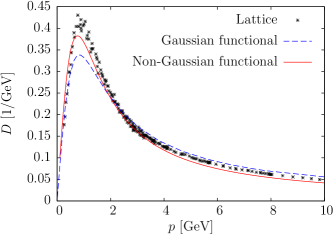
Figure 1: The static gluon propagator $D(p)=1/2\omega(p)$ in momentum space. Crosses are lattice data, while the dashed and full lines, respectively, refer to the results of the variational approach with a Gaussian Feuchter and Reinhardt (2004a, b) and a non-Gaussian Campagnari and Reinhardt (2010) vacuum wave functional.

Finally, as shown in ref. Heffner et al. (2012) the Coulomb term is completely irrelevant in the gluon sector, i.e. $H_{\mathrm{C}}^{\mathrm{YM}}$ can be safely neglected. Furthermore, the interaction term $H_{\mathrm{C}}^{\mathrm{INT}}$ contributes to $\langle H_{\mathrm{QCD}}\rangle$ only in higher than two-loop order and will hence be neglected. On the other hand, the quark part $H_{\mathrm{C}}^{\mathrm{Q}}$ (with the Coulomb kernel $\hat{F}$ replaced by its expectation value (30)) contributes already at the two-loop level and has to be kept. We will later find that this term is in fact quite important for the spontaneous breaking of chiral symmetry. The Hamiltonian of the quark sector then reads

$$\bar{H}_{\mathrm{Q}}=H_{\mathrm{Q}}+H_{\mathrm{C}}^{\mathrm{Q}}$$ (34)

with the Coulomb kernel $\hat{F}$ in $H_{\mathrm{C}}^{\mathrm{Q}}$ replaced by its gluonic vacuum expectation value $V_{\mathrm{C}}$ [eq. (30)].

IV The quark wave functional

Our trial ansatz for the quark wave functional is an extension of that used in refs. Pak and Reinhardt (2012, 2013). Following these references, we split the quark field operator $\psi$ into its positive and negative energy components

$$\psi(\boldsymbol{x})=\psi_{+}(\boldsymbol{x})+\psi_{-}(\boldsymbol{x})$$ (35)

defined with respect to the bare Dirac vacuum $|0\rangle$

$$\psi_{+}(\boldsymbol{x})|0\rangle=0=\psi_{-}^{\dagger}(\boldsymbol{x})|0\rangle\,.$$ (36)

The bare Dirac vacuum consists of the filled negative energy eigenstates of the bare Dirac Hamiltonian, which in momentum space reads

$$h(\boldsymbol{p})=\boldsymbol{\alpha}\cdot\boldsymbol{p}+\beta m_{\mathrm{Q}}\,$$ (37)

and whose eigenvalues are given by $\pm e(p)=\pm\sqrt{p^{2}+m_{\mathrm{Q}}^{2}}$. The positive and negative energy components of the quark field can then be expressed as

$$\psi_{\pm}(\boldsymbol{x})=\int\mathrm{d}^{3}y\,\Lambda_{\pm}(\boldsymbol{x},\boldsymbol{y})\psi(\boldsymbol{y})$$ (38)

with the orthogonal projectors ($\mathop{\mathrm{d}\mkern-7.0mu\mathchar 22\relax\mkern-1.0mu}\mkern-4.0mu=\mathrm{d}/(2\pi)$)

$$\Lambda_{\pm}(\boldsymbol{x},\boldsymbol{y})=\int\mathop{\mathrm{d}\mkern-7.0mu\mathchar 22\relax\mkern-1.0mu}\mkern-4.0mu^{3}p\,\exp\bigl{(}\mathrm{i}\boldsymbol{p}\cdot(\boldsymbol{x}-\boldsymbol{y})\bigr{)}\Lambda_{\pm}(\boldsymbol{p})\,,\quad\quad\Lambda_{\pm}(\boldsymbol{p})=\frac{1}{2}\left(\mathbbm{1}\pm\frac{h(\boldsymbol{p})}{e(p)}\right)$$ (39)

satisfying

$$\Lambda_{+}+\Lambda_{-}=\mathbbm{1}\,,\quad\quad\Lambda_{\pm}^{2}=\Lambda_{\pm}\,,\quad\quad\Lambda_{\pm}\Lambda_{\mp}=0\,.$$ (40)

From (10) it follows that the projected quark fields $\psi_{\pm}$ obey the anti-commutation relations

$$\left\{\psi_{\pm}(\boldsymbol{x}),\psi_{\pm}^{\dagger}(\boldsymbol{y})\right\} =\Lambda_{\pm}(\boldsymbol{x},\boldsymbol{y})\,, \quad\quad\left\{\psi_{\pm}(\boldsymbol{x}),\psi_{\mp}^{\dagger}(\boldsymbol{y})\right\} =0$$ (41a)

$$\Bigl{\{}\psi_{\pm}(\boldsymbol{x}),\psi_{\pm}(\boldsymbol{y})\Bigr{\}} =0\,, \quad\quad\Bigl{\{}\psi_{\pm}(\boldsymbol{x}),\psi_{\mp}(\boldsymbol{y})\Bigr{\}} =0\,.$$ (41b)

In the following, we will consider only the limit of chiral quarks, i.e. $m_{\mathrm{Q}}=0$. The extension of our ansatz to massive quarks would be, however, straightforward. The quark trial vacuum state is chosen as the most general Slater determinant which is not orthogonal to the bare vacuum $|0\rangle$. By Thouless’s theorem such a state can be expressed as

$$|\phi_{\mathrm{Q}}[A]\rangle=\exp\left[-\int\mathrm{d}^{3}x\int\mathrm{d}^{3}y\,\psi_{+}^{\dagger}(\boldsymbol{x})K(\boldsymbol{x},\boldsymbol{y})\psi_{-}(\boldsymbol{y})\right]|0\rangle\,,$$ (42)

where the (gauge field dependent) kernel $K$ is a matrix in the indices of the quark fields, i.e. in Lorentz and color space and, when different flavors are included, also in flavor space. The use of a Slater determinant allows the application of Wick’s theorem, which facilitates the evaluation of the quark expectation value considerably. The norm of the fermionic wave functional (42) is given by Pak and Reinhardt (2013)

$$I[A]\equiv\langle\phi_{\mathrm{Q}}[A]|\phi_{\mathrm{Q}}[A]\rangle=\det\begin{pmatrix}\mathbbm{1}&K\\ K^{\dagger}&-\mathbbm{1}\end{pmatrix}=\det\bigl{(}\mathbbm{1}+K^{\dagger}K\bigr{)}\,,$$ (43)

where the first (functional) determinant is defined in the complete Hilbert space of the Dirac Hamiltonian (37), while the second one is defined in the subspace of negative energy eigenfunctions only. Note that the fermion determinant $I[A]$ [eq. (43)] explicitly depends on the gauge field $A$ and is therefore non-trivial. The kernel $K$ connects the positive with the negative energy subspace of the (single particle) Hilbert space of the Dirac Hamiltonian (37) and is chosen in the form

$$K(\boldsymbol{x},\boldsymbol{y})=\beta S(\boldsymbol{x},\boldsymbol{y})+g\int\mathrm{d}^{3}z\,\bigl{[}V(\boldsymbol{x},\boldsymbol{y};\boldsymbol{z})+\beta W(\boldsymbol{x},\boldsymbol{y};\boldsymbol{z})\bigr{]}\boldsymbol{\alpha}\cdot\boldsymbol{A}^{a}(\boldsymbol{z})t^{a}\,,$$ (44)

where $S$, $V$ and $W$ are variational kernels, which, by translational invariance, depend only on the coordinate differences. For $V=W=0$ our ansatz $|\phi_{\mathrm{Q}}[A]\rangle$ [eq. (42)] reduces to the BCS-type wave functional considered in refs. Finger and Mandula (1982); Adler and Davis (1984); Alkofer and Amundsen (1988). For the BCS-wave functional the quark-gluon coupling term of the Dirac Hamiltonian, $H_{\mathrm{Q}}^{A}$ [eq. (9)], escapes the expectation value. Such a wave functional does, however, already produce spontaneous breaking of chiral symmetry but not of sufficient amount. It yields, for $\sigma_{\mathrm{C}}=2\sigma$, a quark condensate $\langle\bar{\psi}\psi\rangle$ of about $(-165\,\mathrm{MeV})^{3}$ which is significantly smaller than the phenomenological value of Williams et al. (2007)

$$\langle\bar{\psi}(\boldsymbol{x})\psi(\boldsymbol{x})\rangle_{\mathrm{phen}}=(-235\,\mathrm{MeV})^{3}\,.$$ (45)

For $W=0$ the wave functional (42) corresponds to the ansatz considered in refs. Pak and Reinhardt (2012, 2013), where it was shown that the inclusion of the explicit coupling of the quarks to the gluons by the term proportional to $V$ gives a substantial improvement compared to the BCS-type wave functional ($V=W=0$). Here we go one step further and include also the coupling term proportional to $W$. As we will show below this term does not only improve the previous variational calculation because of the enlarged space of trial states but has the principle advantage that all linear ultraviolet divergences disappear from the gap equation for the scalar kernel $S$. Furthermore, the presence of this kernel can be motivated by perturbation theory on top of a BCS-vacuum state, see appendix B.

It is convenient to include the fermion determinant $I$ [eq. (43)] in our ansatz for the Yang–Mills part $\phi_{\mathrm{YM}}$ of the vacuum wave functional (22) in the same way as the Faddeev–Popov determinant $J$. Therefore, we choose the following ansatz

$$\phi_{\mathrm{YM}}[A] =\mathcal{N}I^{-\frac{1}{2}}[A]J^{-\frac{1}{2}}[A]\widetilde{\phi}_{\mathrm{YM}}[A]\,,$$ (46a)

$$\widetilde{\phi}_{\mathrm{YM}}[A] =\exp\left(-\frac{1}{2}\int\mathrm{d}^{3}x\int\mathrm{d}^{3}y\,A_{k}^{a}(\boldsymbol{x})\omega(\boldsymbol{x},\boldsymbol{y})A_{k}^{a}(\boldsymbol{y})\right)\,,$$ (46b)

which differs from (24) only by the presence of the fermion determinant. Again, $\omega$ is the variational kernel to be determined by minimizing the ground state energy. In terms of the functional (46) the expectation value of an arbitrary operator $O$ [eq. (23)] reads

$$\langle O[A,\Pi,\psi]\rangle=|\mathcal{N}|^{2}\int\mathcal{D}A\,\widetilde{\phi}^{*}_{\mathrm{YM}}[A]\langle\widetilde{O}[A,\Pi,\psi]\rangle_{\mathrm{Q}}\,\widetilde{\phi}_{\mathrm{YM}}[A]$$ (47)

where we have introduced the transformed operator

$$\widetilde{O}[A,\Pi,\psi]\equiv J^{\frac{1}{2}}[A]I^{\frac{1}{2}}[A]O[A,\Pi,\psi]J^{-\frac{1}{2}}[A]I^{-\frac{1}{2}}[A]$$ (48)

and the fermionic expectation value

$$\langle O\rangle_{\mathrm{Q}}=I^{-1}\langle\phi_{\mathrm{Q}}|O|\phi_{\mathrm{Q}}\rangle\,.$$ (49)

For an operator $O$ which is independent of the canonical momentum $\Pi$, $O=\widetilde{O}$ holds and both the Faddeev–Popov and the fermion determinants disappear from the expectation value (47) implying that Wick’s theorem holds in the form

$$\langle O[A,\psi]\rangle=\left.\left\{\exp\left(\frac{1}{2}\int\mathrm{d}^{3}x\int\mathrm{d}^{3}y\,\frac{\delta}{\delta A_{k}^{a}(\boldsymbol{x})}D_{kl}^{ab}(\boldsymbol{x},\boldsymbol{y})\frac{\delta}{\delta A_{l}^{b}(\boldsymbol{y})}\right)\langle O[A,\psi]\rangle_{\mathrm{Q}}\right\}\right|_{A=0}\,.$$ (50)

If, however, the operator $O$ explicitly depends on the canonical momentum operator, the Faddeev–Popov determinant $J$ and the fermion determinant $I$ remain in the expectation value (47), (48) and the functional derivative imposed by the momentum operator $\Pi=\delta/\mathrm{i}\delta A$ has to be carried out before Wick’s theorem can be applied.

V Static quark propagator and chiral condensate

Since our quark wave functional is a Gaussian in the fermion fields Wick’s theorem holds and as a consequence pure fermionic expectation values can be expressed in terms of the static quark propagator

$$G_{ij}^{mn}(\boldsymbol{x},\boldsymbol{y})=\frac{1}{2}\langle\Bigl{[}\psi_{i}^{m}(\boldsymbol{x}),{\psi_{j}^{n}}^{\dagger}(\boldsymbol{y})\Bigr{]}\rangle\,.$$ (51)

For the fermionic expectation value of the quark bilinear in the state $|\phi_{\mathrm{Q}}[A]\rangle$ [eq. (42)] one finds Pak and Reinhardt (2013)

$$\langle\psi_{+,i}(\boldsymbol{x})\psi_{+,j}^{\dagger}(\boldsymbol{y})\rangle_{\mathrm{Q}} =\bigl{(}\Lambda_{+}\bigl{[}\mathbbm{1}+KK^{\dagger}\bigr{]}^{-1}\Lambda_{+}\bigr{)}_{ij}(\boldsymbol{x},\boldsymbol{y})\,,$$ (52a)

$$\langle\psi_{-,i}^{\dagger}(\boldsymbol{x})\psi_{-,j}(\boldsymbol{y})\rangle_{\mathrm{Q}} =\bigl{(}\Lambda_{-}\bigl{[}\mathbbm{1}+K^{\dagger}K\bigr{]}^{-1}\Lambda_{-})_{ji}(\boldsymbol{y},\boldsymbol{x})\,,$$ (52b)

$$\langle\psi_{-,i}(\boldsymbol{x})\psi_{+,j}^{\dagger}(\boldsymbol{y})\rangle_{\mathrm{Q}} =\bigl{(}\Lambda_{-}\bigl{[}\mathbbm{1}+K^{\dagger}K]^{-1}K^{\dagger}\Lambda_{+}\bigr{)}_{ij}(\boldsymbol{x},\boldsymbol{y})\,,$$ (52c)

$$\langle\psi_{+,i}(\boldsymbol{x})\psi_{-,j}^{\dagger}(\boldsymbol{y})\rangle_{\mathrm{Q}} =\bigl{(}\Lambda_{+}\bigl{[}\mathbbm{1}+KK^{\dagger}]^{-1}K\Lambda_{-})_{ij}(\boldsymbol{x},\boldsymbol{y})\,.$$ (52d)

Unfortunately, the evaluation of the bosonic expectation value is a bit more involved and cannot be carried out without further approximations. This is because the fermionic two-point functions always contain a term like

$$\left[\mathbbm{1}+KK^{\dagger}\right]^{-1}=\sum_{n=0}^{\infty}(-1)^{n}\left(KK^{\dagger}\right)^{n}$$ (53)

which is an infinite series in the gauge field $A$ so that its bosonic expectation value cannot be evaluated in closed form. For calculating the ground state energy up to two-loop order, it is sufficient to expand the exponential in (50) in a Taylor series up to leading order yielding

$$\langle O[A,\psi]\rangle\approx\langle O[A=0,\psi]\rangle_{\mathrm{Q}}+\frac{1}{2}\int\mathrm{d}^{3}x\int\mathrm{d}^{3}y\,\frac{\delta}{\delta A_{k}^{a}(\boldsymbol{x})}D_{kl}^{ab}(\boldsymbol{x},\boldsymbol{y})\frac{\delta}{\delta A_{l}^{b}(\boldsymbol{y})}\langle O[A,\psi]\rangle_{\mathrm{Q}}\Bigr{|}_{A=0}.$$ (54)

For the static quark propagator

$$G_{ij}^{mn}(\boldsymbol{x},\boldsymbol{y})=\delta^{mn}\int\mathop{\mathrm{d}\mkern-7.0mu\mathchar 22\relax\mkern-1.0mu}\mkern-4.0mu^{3}p\,\exp\bigl{(}\mathrm{i}\boldsymbol{p}\cdot(\boldsymbol{x}-\boldsymbol{y})\bigr{)}G_{ij}(\boldsymbol{p})$$ (55)

in momentum space we find then after somewhat lengthy calculations, see appendix C,

$$G(\boldsymbol{p})=\frac{P(p)}{2}\Bigl{[}1-S^{2}(p)-I_{\alpha}(p)\Bigr{]}\boldsymbol{\alpha}\cdot\hat{\boldsymbol{p}}+P(p)\Bigl{[}S(p)-I_{\beta}(p)\Bigr{]}\beta$$ (56)

where $\hat{\boldsymbol{p}}=\boldsymbol{p}/p$ and

$$I_{\alpha}(p) =C_{\mathrm{F}}g^{2}\int\mathop{\mathrm{d}\mkern-7.0mu\mathchar 22\relax\mkern-1.0mu}\mkern-4.0mu^{3}q\,\frac{P(p)P(q)}{\omega(|\boldsymbol{p}+\boldsymbol{q}|)}\left[V^{2}(\boldsymbol{p},\boldsymbol{q})X(\boldsymbol{p},\boldsymbol{q})\Bigl{(}1+2S(p)S(q)-S^{2}(p)\Bigr{)}\right.$$

$$\phantom{=}\,\,\phantom{C_{\mathrm{F}}g^{2}\int\mathop{\mathrm{d}\mkern-7.0mu\mathchar 22\relax\mkern-1.0mu}\mkern-4.0mu^{3}q\,\frac{P(p)P(q)}{\omega(|\boldsymbol{p}+\boldsymbol{q}|)}\left[\right.}\left.+W^{2}(\boldsymbol{p},\boldsymbol{q})Y(\boldsymbol{p},\boldsymbol{q})\Bigl{(}1-2S(p)S(q)-S^{2}(p)\Bigr{)}\right]$$ (57)

$$I_{\beta}(p) =\frac{C_{\mathrm{F}}}{2}g^{2}\int\mathop{\mathrm{d}\mkern-7.0mu\mathchar 22\relax\mkern-1.0mu}\mkern-4.0mu^{3}q\,\frac{P(p)P(q)}{\omega(|\boldsymbol{p}+\boldsymbol{q}|)}\left[V^{2}(\boldsymbol{p},\boldsymbol{q})X(\boldsymbol{p},\boldsymbol{q})\Bigl{(}2S(p)-S(q)+S^{2}(p)S(q)\Bigr{)}\right.$$

$$\phantom{=}\,\,\phantom{\frac{C_{\mathrm{F}}}{2}g^{2}\int\mathop{\mathrm{d}\mkern-7.0mu\mathchar 22\relax\mkern-1.0mu}\mkern-4.0mu^{3}q\,\frac{P(p)P(q)}{\omega(|\boldsymbol{p}+\boldsymbol{q}|)}\left[\right.}\left.+W^{2}(\boldsymbol{p},\boldsymbol{q})Y(\boldsymbol{p},\boldsymbol{q})\Bigl{(}2S(p)+S(q)-S^{2}(p)S(q)\Bigr{)}\right].$$ (58)

Here we have replaced the variational kernels by their respective momentum space representation, see appendix A, and, furthermore, introduced the abbreviations

$$P(p) =\frac{1}{1+S^{2}(p)}$$ (59)

$$X(\boldsymbol{p},\boldsymbol{q}) =1-\Bigl{[}\hat{\boldsymbol{p}}\cdot\widehat{(\boldsymbol{p}+\boldsymbol{q})}\Bigr{]}\Bigl{[}\hat{\boldsymbol{q}}\cdot\widehat{(\boldsymbol{p}+\boldsymbol{q})}\Bigr{]}$$ (60)

$$Y(\boldsymbol{p},\boldsymbol{q}) =1+\Bigl{[}\hat{\boldsymbol{p}}\cdot\widehat{(\boldsymbol{p}+\boldsymbol{q})}\Bigr{]}\Bigl{[}\hat{\boldsymbol{q}}\cdot\widehat{(\boldsymbol{p}+\boldsymbol{q})}\Bigr{]}$$ (61)

as well as the Casimir factor $C_{\mathrm{F}}=(N_{\mathrm{C}}^{2}-1)/2N_{\mathrm{C}}$. Neglecting the coupling of the quarks to the transversal gluons, $V=W=0$, the propagator (56) reduces to the BCS result obtained in ref. Adler and Davis (1984). However, even when we include the coupling term $\sim V$ but ignore the additional coupling term $\sim W$ our quark propagator differs from that of ref. Pak and Reinhardt (2013), although in that case the trial ansätze for the quark wave functional agree. The reason is that in ref. Pak and Reinhardt (2013) a simplifying approximation was used in the evaluation of the gluonic expectation value of fermionic objects: In the denominators of the quark propagator (52) the kernel $K^{\dagger}K$ was replaced by its (gluonic) vacuum expectation value $\langle K^{\dagger}K\rangle$. In the present paper we abandoned this approximation and strictly carried out the calculation to two-loop order. The results obtained in this way are also consistent with those obtained in the Dyson–Schwinger approach Campagnari and Reinhardt (shed) and in perturbation theory, as we will see later.

Due to the fact that our quark wave functional is a Slater determinant the static quark propagator (56) can be brought to the quasi-particle form

$$G(\boldsymbol{p})=Z(p)\frac{\boldsymbol{\alpha}\cdot\boldsymbol{p}+\beta M(\boldsymbol{p})}{2\sqrt{p^{2}+M^{2}(p)}}$$ (62)

with an effective (running) mass

$$M(p)=\frac{2p\bigl{[}S(p)-I_{\beta}(p)\bigr{]}}{1-S^{2}(p)-I_{\alpha}(p)}$$ (63)

and a field renormalization factor

$$Z(p)=P(p)\sqrt{\bigl{[}1-S^{2}(p)-I_{\alpha}(p)\bigr{]}^{2}+4\bigl{[}S(p)-I_{\beta}(p)\bigr{]}^{2}}\,.$$ (64)

If one neglects the coupling of the quarks to the gluons the two loop integrals vanish, $I_{\alpha}=I_{\beta}=0$, and we recover the result of ref. Adler and Davis (1984)

$$M(p)=\frac{2pS(p)}{1-S^{2}(p)},\quad\quad Z(p)=1\,.$$ (65)

From this expression it is already clear that a non-vanishing scalar kernel $S$ implies a non-zero effective quark mass function and thus spontaneous breaking of chiral symmetry. Indeed the order parameter of spontaneous breaking of chiral symmetry, the quark condensate, can be expressed by means of the static quark propagator (51) as

$$\langle\bar{\psi}(\boldsymbol{x})\psi(\boldsymbol{x})\rangle=-\mathrm{tr}\bigl{(}\beta G(\boldsymbol{x},\boldsymbol{x})\bigr{)}\,.$$ (66)

Inserting here the explicit form of the propagator (62) we find

$$\langle\bar{\psi}(\boldsymbol{x})\psi(\boldsymbol{x})\rangle=-2\int\mathop{\mathrm{d}\mkern-7.0mu\mathchar 22\relax\mkern-1.0mu}\mkern-4.0mu^{3}p\,\frac{Z(\boldsymbol{p})M(\boldsymbol{p})}{\sqrt{p^{2}+M^{2}(\boldsymbol{p})}}\,.$$ (67)

Obviously, the quark condensate vanishes when no effective mass is generated, i.e. for $M=0$.

VI Ground state energy

Below we evaluate the expectation value of the QCD Hamiltonian (18) in our trial state (22) [with eqs. (42) and (46)]. The calculations will be carried out consistently to two-loop level.

Since the quark wave functional depends explicitly on the gauge field it is mandatory to take the fermionic expectation value before the bosonic one. We begin with the expectation value of the Dirac Hamiltonian $H_{\mathrm{Q}}$.

VI.1 Quark energy

The Dirac Hamiltonian (9) consists of two parts, one describing a free Dirac particle and the other containing the coupling between quarks and transversal gluons. The expectation value of the free Dirac Hamiltonian can be expressed by the quark Green function

$$\langle H_{\mathrm{Q}}^{0}\rangle=-N_{\mathrm{C}}\delta\mkern-8.0mu\mathchar 22\relax^{3}(0)\int\mathop{\mathrm{d}\mkern-7.0mu\mathchar 22\relax\mkern-1.0mu}\mkern-4.0mu^{3}p\,\mathrm{tr}\Bigl{(}\boldsymbol{\alpha}\cdot\boldsymbol{p}\,G(\boldsymbol{p})\Bigr{)}\,,$$ (68)

where $\delta\mkern-8.0mu\mathchar 22\relax^{3}(0)=\int\mathrm{d}^{3}x$ is the (infinite) spatial volume ($\delta\mkern-8.0mu\mathchar 22\relax=2\pi\delta$). With the explicit form (62) we find

$$\langle H_{\mathrm{Q}}^{0}\rangle=-2N_{\mathrm{C}}\delta\mkern-8.0mu\mathchar 22\relax^{3}(0)\int\mathop{\mathrm{d}\mkern-7.0mu\mathchar 22\relax\mkern-1.0mu}\mkern-4.0mu^{3}p\,\frac{p^{2}Z(p)}{\sqrt{p^{2}+M^{2}(p)}}\,.$$ (69)

Here $G$, $M$ and $Z$ are functionals of the variational kernels $S$, $V$ and $W$ [see eqs. (62), (63) and (64)]. Using the explicit expression for these quantities one finds for $\langle H_{\mathrm{Q}}^{0}\rangle$ a somewhat lengthy expression, which is given in eq. (157) of appendix D. The obtained expression for $\langle H_{\mathrm{Q}}^{0}\rangle$ allows, however, for a direct interpretation in terms of Feynman diagrams given in fig. 2.

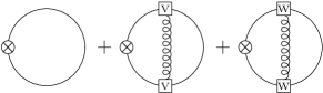
Figure 2: Diagrammatic representation of the expectation value of the free Dirac Hamiltonian (69). We denote the free Dirac operator by a crossed circle and the vector kernels $V$ and $W$ by a labeled square. Straight and curly lines stand, respectively, for the quark and gluon propagator.

Let us also mention that there is no need to subtract the energy of the trivial vacuum, $\langle H_{\mathrm{QCD}}\rangle|_{S=V=W=0}$, because this would only shift the vacuum energy by an irrelevant constant.

The evaluation of the coupling term $\langle H_{\mathrm{Q}}^{A}\rangle$ is more involved due to the presence of the gauge field in $H_{\mathrm{Q}}^{A}$ but can be straighforwardly carried out to two loops. One finds then the following expression

$$\langle H_{\mathrm{Q}}^{A}\rangle =-\bigl{(}N_{\mathrm{C}}^{2}-1\bigr{)}\delta\mkern-8.0mu\mathchar 22\relax^{3}(0)g^{2}\int\mathop{\mathrm{d}\mkern-7.0mu\mathchar 22\relax\mkern-1.0mu}\mkern-4.0mu^{3}p\int\mathop{\mathrm{d}\mkern-7.0mu\mathchar 22\relax\mkern-1.0mu}\mkern-4.0mu^{3}q\,\frac{V(\boldsymbol{p},\boldsymbol{q})}{\omega(|\boldsymbol{p}+\boldsymbol{q}|)}P(q)P(p)\Bigl{(}1+S(q)S(p)\Bigr{)}X(\boldsymbol{p},\boldsymbol{q})$$

$$\phantom{=}\,\,-\bigl{(}N_{\mathrm{C}}^{2}-1\bigr{)}\delta\mkern-8.0mu\mathchar 22\relax^{3}(0)g^{2}\int\mathop{\mathrm{d}\mkern-7.0mu\mathchar 22\relax\mkern-1.0mu}\mkern-4.0mu^{3}p\int\mathop{\mathrm{d}\mkern-7.0mu\mathchar 22\relax\mkern-1.0mu}\mkern-4.0mu^{3}q\,\frac{W(\boldsymbol{p},\boldsymbol{q})}{\omega(|\boldsymbol{p}+\boldsymbol{q}|)}P(q)P(p)\Bigl{(}S(p)+S(q)\Bigr{)}Y(\boldsymbol{p},\boldsymbol{q})\,,$$ (70)

which is diagrammatically illustrated in fig. 3.

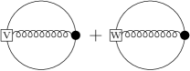
Figure 3: Diagrammatic representation of the expectation value of the quark-gluon coupling, $\langle H_{\mathrm{Q}}^{A}\rangle$ (70). The filled dot stands for the bare quark-gluon vertex in the Hamiltonian $H_{\mathrm{Q}}^{A}$.

The quark contribution to the Coulomb energy $\langle H_{\mathrm{C}}^{\mathrm{Q}}\rangle$ can be straighforwardly evaluated by using Wick’s theorem in the quark sector. Due to the replacement of the Coulomb kernel $\hat{F}$ [eq. (12)] by its expectation value $V_{\mathrm{C}}$ [eq. (30)], which is correct to two-loop order, we are left here with a quark two-body operator $\psi^{\dagger}\psi\,\psi^{\dagger}\psi$, whose fermionic expectation value leads to terms of the form $\langle\psi^{\dagger}\psi\rangle_{\mathrm{Q}}\langle\psi\,\psi^{\dagger}\rangle_{\mathrm{Q}}$. Furthermore, up to two loops the remaining gluonic expectation value can be taken for each fermion contraction $\langle\psi\,\psi^{\dagger}\rangle_{\mathrm{Q}}$ separately, which produces a static quark propagator (51). Exploiting the fact that the quark propagator is a color singlet and that $\mathrm{tr}\,t^{a}=0$ one arrives at the following result

$$\langle H_{\mathrm{C}}^{\mathrm{Q}}\rangle=\frac{1}{8}t_{m_{1}m_{2}}^{a}t_{m_{3}m_{4}}^{a}\int\mathrm{d}^{3}x\int\mathrm{d}^{3}y\,V_{\mathrm{C}}(|\boldsymbol{x}-\boldsymbol{y}|)\Bigl{[}\delta^{m_{1}m_{4}}\delta^{m_{2}m_{3}}\delta_{ii}\delta^{3}(0)\delta^{3}(\boldsymbol{x}-\boldsymbol{y})-4\mathrm{tr}\bigl{(}G^{m_{4}m_{1}}(\boldsymbol{y},\boldsymbol{x})G^{m_{2}m_{3}}(\boldsymbol{x},\boldsymbol{y})\bigr{)}\Bigr{]}\,.$$ (71)

Inserting here the explicit expression for the static quark propagator (56) and confining oneself to two-loop terms yields

$$\langle H_{\mathrm{C}}^{\mathrm{Q}}\rangle=\frac{N_{\mathrm{C}}^{2}-1}{4}\delta\mkern-8.0mu\mathchar 22\relax^{3}(0)\int\mathop{\mathrm{d}\mkern-7.0mu\mathchar 22\relax\mkern-1.0mu}\mkern-4.0mu^{3}p\int\mathop{\mathrm{d}\mkern-7.0mu\mathchar 22\relax\mkern-1.0mu}\mkern-4.0mu^{3}q\,V_{\mathrm{C}}(|\boldsymbol{p}-\boldsymbol{q}|)\Bigl{[}1-P(p)P(q)\Bigl{(}4S(p)S(q)+\bigl{(}1-S^{2}(p)\bigr{)}\bigl{(}1-S^{2}(q)\bigr{)}\hat{\boldsymbol{p}}\cdot\hat{\boldsymbol{q}}\Bigr{)}\Bigr{]}\,.$$ (72)

The same result is found for the BCS-wave functional ($V=W=0$). This is because the quark-gluon coupling vertices in our trial wave functional (42), (44) contribute only loop terms to the static quark propagator, see eq. (56), which, when kept, would produce three-loop terms in $\langle H_{\mathrm{C}}^{\mathrm{Q}}\rangle$. The quark contribution to the Coulomb energy (72) is diagrammatically illustrated in fig. 4.

Figure 4: Diagrammatic representation of the expectation value of the fermionic part of the color Coulomb potential (72). The double line stands for the Coulomb kernel [eq. $V_{\mathrm{C}}$ (30)].

VI.2 Energy of transversal gluons

We continue with the contribution of the kinetic energy of the transversal gluons $H_{\mathrm{YM}}^{E}$, see eq. (2). Although the operator $H_{\mathrm{YM}}^{E}$ does not contain the quark field, the quarks do contribute to its expectation value due to the action of the momentum operator on the gauge field in the quark wave functional, see eqs. (42) and (44). Furthermore, the momentum operator does not commute with the fermion determinant (43). As a consequence the transformed operator $\widetilde{H}_{\mathrm{YM}}^{E}$ [eq. (48)] becomes non-trivial

$$\widetilde{H}_{\mathrm{YM}}^{E} =\frac{1}{2}\int\mathop{\mathrm{d}\mkern-7.0mu\mathchar 22\relax\mkern-1.0mu}\mkern-4.0mu^{3}p\left(\Pi_{k}^{a}(\boldsymbol{p})\Pi_{k}^{a}(-\boldsymbol{p})-\bigl{[}\Pi_{k}^{a}(\boldsymbol{p})\ln I\bigr{]}\Pi_{k}^{a}(-\boldsymbol{p})-\frac{1}{4}\bigl{[}\Pi_{k}^{a}(\boldsymbol{p})\ln J\bigr{]}\bigl{[}\Pi_{k}^{a}(-\boldsymbol{p})\ln J\bigr{]}\right.$$

$$\phantom{=}\,\,\quad\quad+\left.\frac{1}{4}\bigl{[}\Pi_{k}^{a}(\boldsymbol{p})\ln I\bigr{]}\bigl{[}\Pi_{k}^{a}(-\boldsymbol{p})\ln I\bigr{]}-\frac{1}{2}\bigl{[}\Pi_{k}^{a}(\boldsymbol{p})\Pi_{k}^{a}(-\boldsymbol{p})\ln J\bigr{]}-\frac{1}{2}\bigl{[}\Pi_{k}^{a}(\boldsymbol{p})\Pi_{k}^{a}(-\boldsymbol{p})\ln I\bigr{]}\right).$$ (73)

Obviously this transformed operator has a much more complicated structure than the original one. This is the price we have to pay for the elimination of the Faddeev–Popov and quark determinants from the gluonic integration measure of the scalar product, see eq. (47). The evaluation of the expectation value of $\widetilde{H}_{\mathrm{YM}}^{E}$ [eq. (73)] is quite involved and sketched in appendix D. Up to two-loop order one finds the following expression:

$$\langle H_{\mathrm{YM}}^{E}\rangle =\frac{N_{\mathrm{C}}^{2}-1}{2}\delta\mkern-8.0mu\mathchar 22\relax^{3}(0)\int\mathop{\mathrm{d}\mkern-7.0mu\mathchar 22\relax\mkern-1.0mu}\mkern-4.0mu^{3}p\,\frac{\bigl{(}\omega(p)-\chi(p)\bigr{)}^{2}}{\omega(p)}$$

$$\phantom{=}\,\,+\frac{N_{\mathrm{C}}^{2}-1}{2}\delta\mkern-8.0mu\mathchar 22\relax^{3}(0)g^{2}\int\mathop{\mathrm{d}\mkern-7.0mu\mathchar 22\relax\mkern-1.0mu}\mkern-4.0mu^{3}p\int\mathop{\mathrm{d}\mkern-7.0mu\mathchar 22\relax\mkern-1.0mu}\mkern-4.0mu^{3}q\,P(p)P(q)V^{2}(\boldsymbol{p},\boldsymbol{q})X(\boldsymbol{p},\boldsymbol{q})$$

$$\phantom{=}\,\,+\frac{N_{\mathrm{C}}^{2}-1}{2}\delta\mkern-8.0mu\mathchar 22\relax^{3}(0)g^{2}\int\mathop{\mathrm{d}\mkern-7.0mu\mathchar 22\relax\mkern-1.0mu}\mkern-4.0mu^{3}p\int\mathop{\mathrm{d}\mkern-7.0mu\mathchar 22\relax\mkern-1.0mu}\mkern-4.0mu^{3}q\,P(p)P(q)W^{2}(\boldsymbol{p},\boldsymbol{q})Y(\boldsymbol{p},\boldsymbol{q})$$ (74)

Here $\chi(p)=\delta^{ab}\mathrm{tr}\,t(\boldsymbol{p})\chi^{ab}(\boldsymbol{p})/(2(N_{\mathrm{C}}^{2}-1))$ is the scalar curvature. The first term in eq. (74) arises from the Yang–Mills part of the vacuum wave functional and was already obtained in ref. Feuchter and Reinhardt (2004a, b). The last two terms give the quark contributions which are diagrammatically represented in fig. 5.

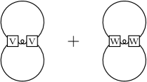
Figure 5: Diagrammatic representation of the fermionic contributions to the expectation value of the kinetic energy of the transversal gluons (74).

The potential energy of the transversal gluons $H_{\mathrm{YM}}^{B}$ [eq. (2)] is a functional of the gauge field $A$ only. As a consequence the quarks do not contribute to $\langle H_{\mathrm{YM}}^{B}\rangle$ which is hence given by the expresson obtained in ref. Feuchter and Reinhardt (2004a, b) for the Yang–Mills sector

$$\langle{H}_{\mathrm{YM}}^{B}\rangle=\frac{N_{\mathrm{C}}^{2}-1}{2}\delta\mkern-8.0mu\mathchar 22\relax^{3}(0)\int\mathop{\mathrm{d}\mkern-7.0mu\mathchar 22\relax\mkern-1.0mu}\mkern-4.0mu^{3}p\,\frac{p^{2}}{\omega(p)}+\frac{N_{\mathrm{C}}\left(N_{\mathrm{C}}^{2}-1\right)}{16}\delta\mkern-8.0mu\mathchar 22\relax^{3}(0)g^{2}\int\mathop{\mathrm{d}\mkern-7.0mu\mathchar 22\relax\mkern-1.0mu}\mkern-4.0mu^{3}p\int\mathop{\mathrm{d}\mkern-7.0mu\mathchar 22\relax\mkern-1.0mu}\mkern-4.0mu^{3}q\,\frac{3-\left(\hat{\boldsymbol{p}}\cdot\hat{\boldsymbol{q}}\right)^{2}}{\omega(p)\omega(q)}\,.$$ (75)

Finally, we calculate the expectation value of the purely gluonic part of the Coulomb term, $H_{\mathrm{C}}^{\mathrm{YM}}$. Although this operator contains the momentum operator $\Pi$ the quarks do not contribute to two-loop order and we obtain the same result as in pure Yang–Mills theory Feuchter and Reinhardt (2004a, b)

$$\langle H_{\mathrm{C}}^{\mathrm{YM}}\rangle=\frac{N_{\mathrm{C}}\left(N_{\mathrm{C}}^{2}-1\right)}{16}\delta\mkern-8.0mu\mathchar 22\relax^{3}(0)\int\mathop{\mathrm{d}\mkern-7.0mu\mathchar 22\relax\mkern-1.0mu}\mkern-4.0mu^{3}p\int\mathop{\mathrm{d}\mkern-7.0mu\mathchar 22\relax\mkern-1.0mu}\mkern-4.0mu^{3}q\,V_{\mathrm{C}}(|\boldsymbol{p}-\boldsymbol{q}|)\frac{\bigl{(}\omega(p)-\chi(p)-\omega(q)+\chi(q)\bigr{)}^{2}}{\omega(p)\omega(q)}\left(1+\left(\hat{\boldsymbol{p}}\cdot\hat{\boldsymbol{q}}\right)^{2}\right)\,.$$ (76)

VI.3 Total energy

As already mentioned before, the mixed Coulomb term $H_{\mathrm{C}}^{\mathrm{INT}}$ does not contribute to two-loop order. The total vacuum energy is thus given by

$$\langle H_{\mathrm{QCD}}\rangle=\langle\bar{H}_{\mathrm{YM}}\rangle+\langle\bar{H}_{\mathrm{Q}}\rangle\,,$$ (77)

where the various contributions to the gluon energy

$$\langle\bar{H}_{\mathrm{YM}}\rangle=\langle H_{\mathrm{YM}}^{E}\rangle+\langle H_{\mathrm{YM}}^{B}\rangle+\langle H_{\mathrm{C}}^{\mathrm{YM}}\rangle$$ (78)

are given by eqs. (74), (75) and (76), while the contribution to the energy of the quarks interacting with the gluons

$$\langle\bar{H}_{\mathrm{Q}}\rangle=\langle H_{\mathrm{Q}}^{0}\rangle+\langle H_{\mathrm{Q}}^{A}\rangle+\langle H_{\mathrm{C}}^{\mathrm{Q}}\rangle$$ (79)

are given by eqs. (69) (see also eq. (157)), (70) and (72). At this point it is worth to compare the present result with that of previous work. If one neglects the coupling between quarks and transversal gluons, $V=W=0$, $\langle\bar{H}_{\mathrm{YM}}\rangle$ becomes the vacuum energy of the Yang–Mills sector obtained in ref. Feuchter and Reinhardt (2004a, b) and $\langle\bar{H}_{\mathrm{Q}}\rangle$ reduces to the vacuum energy of the model considered in ref. Adler and Davis (1984). When the quark-gluon coupling term $\sim V$ is included but the other coupling term ignored, $W=0$, one recovers the result of the Dyson–Schwinger approach of ref. Campagnari and Reinhardt (shed), which differs, however, from the result of ref. Pak and Reinhardt (2013) due to further simplifying approximations used there, see above. Finally, when both quark-gluon coupling terms are included in the quark wave functional but the trivial solution of the gap equation $S=0$ is assumed one recovers from $\langle\bar{H}_{\mathrm{Q}}\rangle$ the quark energy in second order perturbation theory Campagnari and Reinhardt (2015b).

VII Variational equations

Our ansatz for the vacuum functional [(22) with (42) and (46)] contains four variational kernels $\omega$, $S$, $V$ and $W$, which we will determine in the following according to the variational principle. From $\delta\langle H_{\mathrm{QCD}}\rangle/\delta S(k)=0$ we find the following integral equation

$$kS(k)=I_{\mathrm{C}}^{\mathrm{Q}}(k)+I_{VV}^{\mathrm{Q}}(k)+I_{WW}^{\mathrm{Q}}(k)+I_{V\mathrm{Q}}^{\mathrm{Q}}(k)+I_{W\mathrm{Q}}^{\mathrm{Q}}(k)+I_{E}^{\mathrm{Q}}(k)\,,$$ (80)

to which we will refer as quark gap equation. Here

$$I_{\mathrm{C}}^{\mathrm{Q}}(k)=\frac{C_{\mathrm{F}}}{2}\int\mathop{\mathrm{d}\mkern-7.0mu\mathchar 22\relax\mkern-1.0mu}\mkern-4.0mu^{3}p\,V_{\mathrm{C}}(|\boldsymbol{p}-\boldsymbol{k}|)P(p)\left[S(p)\bigl{(}1-S^{2}(k)\bigr{)}-S(k)\bigl{(}1-S^{2}(p)\bigr{)}\hat{\boldsymbol{p}}\cdot\hat{\boldsymbol{k}}\right]$$ (81)

Figure 6: Diagrammatic representation of the contribution (81) of the Coulomb potential to the quark gap equation.

is the contribution from the Coulomb term $H_{\mathrm{C}}^{\mathrm{Q}}$ which is illustrated in fig. 6. Only this term survives when the coupling of the quarks to the transversal gluons in the vacuum wave functional is switched off ($V=W=0$). Furthermore,

$$I_{VV}^{\mathrm{Q}}(k) =-\frac{C_{\mathrm{F}}}{2}g^{2}\int\mathop{\mathrm{d}\mkern-7.0mu\mathchar 22\relax\mkern-1.0mu}\mkern-4.0mu^{3}p\,\frac{V^{2}(\boldsymbol{p},\boldsymbol{k})}{\omega(|\boldsymbol{p}+\boldsymbol{k}|)}X(\boldsymbol{p},\boldsymbol{k})P(p)\Bigl{\{}kP(k)S(k)\Bigl{[}-3+S^{2}(k)\Bigr{]}+pP(p)S(k)\Bigl{[}-1+S^{2}(p)\Bigr{]}$$

$$\phantom{=}\,\,\phantom{-\frac{C_{\mathrm{F}}}{2}g^{2}\int\mathop{\mathrm{d}\mkern-7.0mu\mathchar 22\relax\mkern-1.0mu}\mkern-4.0mu^{3}p\,\times\Bigl{\{}}+kP(k)S(p)\Bigl{[}1-3S^{2}(k)\Bigr{]}+pP(p)S(p)\Bigl{[}1-S^{2}(k)\Bigr{]}\Bigr{\}}$$ (82)

and

$$I_{WW}^{\mathrm{Q}}(k) =-\frac{C_{\mathrm{F}}}{2}g^{2}\int\mathop{\mathrm{d}\mkern-7.0mu\mathchar 22\relax\mkern-1.0mu}\mkern-4.0mu^{3}p\,\frac{W^{2}(\boldsymbol{p},\boldsymbol{k})}{\omega(|\boldsymbol{p}+\boldsymbol{k}|)}Y(\boldsymbol{p},\boldsymbol{k})P(p)\Bigl{\{}kP(k)S(k)\Bigl{[}-3+S^{2}(k)\Bigr{]}+pP(p)S(k)\Bigl{[}-1+S^{2}(p)\Bigr{]}$$

$$\phantom{=}\,\,\phantom{-\frac{C_{\mathrm{F}}}{2}g^{2}\int\mathop{\mathrm{d}\mkern-7.0mu\mathchar 22\relax\mkern-1.0mu}\mkern-4.0mu^{3}p\,\times\Bigl{\{}}-kP(k)S(p)\Bigl{[}1-3S^{2}(k)\Bigr{]}-pP(p)S(p)\Bigl{[}1-S^{2}(k)\Bigr{]}\Bigr{\}}$$ (83)

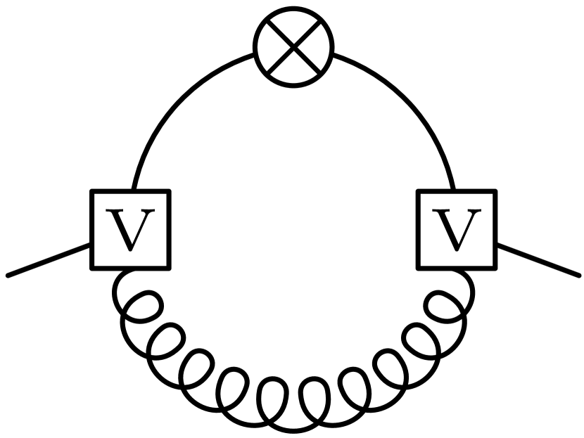
(a)

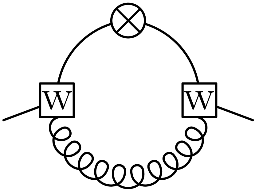
(b)

Figure 7: Diagrammatic representation of the contribution of the free Dirac Hamiltonian to the quark gap equation, (a) eq. (82) and (b) eq. (83).

result from the two-loop contribution of the free Dirac operator to the vacuum energy. These terms are graphically illustrated in fig. 7. The quark-gluon coupling in the Dirac Hamiltonian gives rise to the two diagrams shown in fig. 8 with either a $V$- or a $W$-vertex. Their contributions to the quark gap equation (80) read

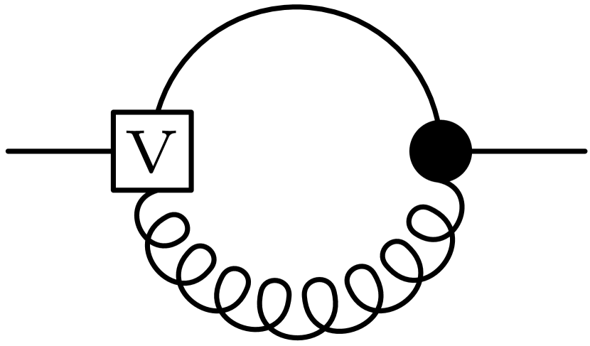
(a)

(b)

Figure 8: Diagrammatic representation of the contribution of the quark-gluon coupling in the Dirac Hamiltonian to the quark gap equation, (a) eq. (84) and (b) eq. (85).

$$I_{V\mathrm{Q}}^{\mathrm{Q}}(k) =\frac{C_{\mathrm{F}}}{2}g^{2}\int\mathop{\mathrm{d}\mkern-7.0mu\mathchar 22\relax\mkern-1.0mu}\mkern-4.0mu^{3}p\,\frac{V(\boldsymbol{p},\boldsymbol{k})}{\omega(|\boldsymbol{p}+\boldsymbol{k}|)}X(\boldsymbol{p},\boldsymbol{k})P(p)\Bigl{[}S(p)\bigl{(}1-S^{2}(k)\bigr{)}-2S(k)\Bigr{]}$$ (84)

$$I_{W\mathrm{Q}}^{\mathrm{Q}}(k) =\frac{C_{\mathrm{F}}}{2}g^{2}\int\mathop{\mathrm{d}\mkern-7.0mu\mathchar 22\relax\mkern-1.0mu}\mkern-4.0mu^{3}p\,\frac{W(\boldsymbol{p},\boldsymbol{k})}{\omega(|\boldsymbol{p}+\boldsymbol{k}|)}Y(\boldsymbol{p},\boldsymbol{k})P(p)\Bigl{[}1-S^{2}(k)-2S(k)S(p)\Bigr{]}\,.$$ (85)

Finally,

$$I_{E}^{\mathrm{Q}}(k)=\frac{C_{\mathrm{F}}}{2}g^{2}S(k)\int\mathop{\mathrm{d}\mkern-7.0mu\mathchar 22\relax\mkern-1.0mu}\mkern-4.0mu^{3}p\,V^{2}(\boldsymbol{p},\boldsymbol{k})X(\boldsymbol{p},\boldsymbol{k})P(p)+\frac{C_{\mathrm{F}}}{2}g^{2}S(k)\int\mathop{\mathrm{d}\mkern-7.0mu\mathchar 22\relax\mkern-1.0mu}\mkern-4.0mu^{3}p\,W^{2}(\boldsymbol{p},\boldsymbol{k})Y(\boldsymbol{p},\boldsymbol{k})P(p)$$ (86)

arises from the quark contribution to the kinetic energy of the transversal gluons [see the last two terms on the r.h.s. of eq. (74)] and is illustrated in fig. 9.

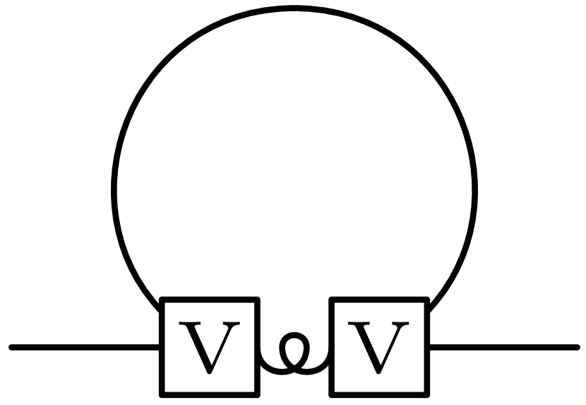
(a)

(b)

Figure 9: Diagrammatic representation of the contribution of the kinetic energy of the transversal gluons to the quark gap equation. (a) and (b) correspond, respectively, to the first and second term on the r.h.s. of eq. (86).

Neglecting the coupling between quarks and transversal gluons, $V=W=0$, the quark gap equation (80) reduces to the one obtained with a BCS-ansatz for the vacuum wave functional Adler and Davis (1984).

The variation with respect to the vector kernel $V$, $\delta\langle H_{\mathrm{QCD}}\rangle/\delta V(\boldsymbol{k},\boldsymbol{k}^{\prime})=0$, leads to an equation which can be explicitly solved for $V(\boldsymbol{k},\boldsymbol{k}^{\prime})$ yielding

$$V(\boldsymbol{k},\boldsymbol{k}^{\prime})=\frac{1+S(k)S(k^{\prime})}{kP(k)\Bigl{(}1-S^{2}(k)+2S(k)S(k^{\prime})\Bigr{)}+k^{\prime}P(k^{\prime})\Bigl{(}1-S^{2}(k^{\prime})+2S(k)S(k^{\prime})\Bigr{)}+\omega(|\boldsymbol{k}+\boldsymbol{k}^{\prime}|)}\,.$$ (87)

This result differs drastically from the one obtained in ref. Pak and Reinhardt (2013), where an integral equation for $V$ was obtained which could not be explictly solved. Furthermore, the vector kernel obtained there depends only on a single momentum argument. However, the quark-gluon vertex connecting three fields should, after taking into account overall momentum conservation, depend on two (independent) momentum arguments, as the vertex (87) does. Finally, for the trivial solution of the gap equation, $S=0$, the expression (87) reduces to the perturbative result Campagnari and Reinhardt (2015b)

$$V_{0}(\boldsymbol{k},\boldsymbol{k}^{\prime})=\frac{1}{k+k^{\prime}+\omega(|\boldsymbol{k}+\boldsymbol{k}^{\prime}|)}\,.$$ (88)

Minimization of the energy density with respect to the second vector kernel $W$ yields an equation which can, again, be solved directly:

$$W(\boldsymbol{k},\boldsymbol{k}^{\prime})=\frac{S(k)+S(k^{\prime})}{kP(k)\Bigl{(}1-S^{2}(k)-2S(k)S(k^{\prime})\Bigr{)}+k^{\prime}P(k^{\prime})\Bigl{(}1-S^{2}(k^{\prime})-2S(k)S(k^{\prime})\Bigr{)}+\omega(|\boldsymbol{k}+\boldsymbol{k}^{\prime})|}\,.$$ (89)

As expected, the kernel $W$ also depends on two momenta. Although the structure of this equation is similar to the one for the kernel $V$ [eq. (87)] there is an essential difference: The kernel $W$ [eq. (89)] vanishes in the chirally symmetric phase $S=0$ and is therefore only non-perturbatively realized, while the other vector kernel $V$ [eq. (87)] reduces for $S=0$ to the perturbative expression (88).

Finally, for the bosonic kernel $\omega$ we obtain from $\delta\langle H_{\mathrm{QCD}}\rangle/\delta\omega(k)=0$ the following integral equation

$$\omega^{2}(k)=\omega_{\mathrm{YM}}^{2}(k)+I_{VV}^{\mathrm{YM}}(k)+I_{WW}^{\mathrm{YM}}(k)+I_{V\mathrm{Q}}^{\mathrm{YM}}(k)+I_{W\mathrm{Q}}^{\mathrm{YM}}(k)$$ (90)

where

$$\omega_{\mathrm{YM}}^{2}(k)=k^{2}+\chi^{2}(k)+I_{\mathrm{T}}^{\mathrm{YM}}+I_{\mathrm{C}}^{\mathrm{YM}}(k)$$ (91)

is the contribution from the gluonic energy $\langle\bar{H}_{\mathrm{YM}}\rangle$ with

$$I_{\mathrm{T}}^{\mathrm{YM}}=\frac{2N_{\mathrm{C}}}{3}g^{2}\int\mathop{\mathrm{d}\mkern-7.0mu\mathchar 22\relax\mkern-1.0mu}\mkern-4.0mu^{3}p\,\frac{1}{\omega(p)}$$ (92)

being the gluonic tadpole and

$$I_{\mathrm{C}}^{\mathrm{YM}}(k)=\frac{N_{\mathrm{C}}}{4}\int\mathop{\mathrm{d}\mkern-7.0mu\mathchar 22\relax\mkern-1.0mu}\mkern-4.0mu^{3}p\,V_{\mathrm{C}}(|\boldsymbol{p}-\boldsymbol{k}|)\Bigl{(}1+\bigl{(}\hat{\boldsymbol{p}}\cdot\hat{\boldsymbol{k}}\bigr{)}^{2}\Bigr{)}\frac{\bigl{(}\omega(p)-\chi(p)+\chi(k)\bigr{)}^{2}-\omega^{2}(k)}{\omega(p)}$$ (93)

being the contribution from the gluonic Coulomb term $\langle H_{\mathrm{C}}^{\mathrm{YM}}\rangle$. Equation (91) is obtained as gluonic gap equation when the quark sector is ignored Feuchter and Reinhardt (2004a, b). The quark contributions to the gluon gap equation (90) arise from the two-loop contributions of the free Dirac Hamiltonian (9) to the vacuum energy

$$I_{VV}^{\mathrm{YM}}(k) =2g^{2}\int\mathop{\mathrm{d}\mkern-7.0mu\mathchar 22\relax\mkern-1.0mu}\mkern-4.0mu^{3}p\,V^{2}(\boldsymbol{p},\boldsymbol{k}-\boldsymbol{p})X(\boldsymbol{p},\boldsymbol{k}-\boldsymbol{p})pP^{2}(p)P(|\boldsymbol{k}-\boldsymbol{p}|)\left(1-S^{2}(p)+2S(p)S(|\boldsymbol{k}-\boldsymbol{p}|)\right)$$ (94)

$$I_{WW}^{\mathrm{YM}}(k) =2g^{2}\int\mathop{\mathrm{d}\mkern-7.0mu\mathchar 22\relax\mkern-1.0mu}\mkern-4.0mu^{3}p\,W^{2}(\boldsymbol{p},\boldsymbol{k}-\boldsymbol{p})Y(\boldsymbol{p},\boldsymbol{k}-\boldsymbol{p})pP^{2}(p)P(|\boldsymbol{k}-\boldsymbol{p}|)\left(1-S^{2}(p)-2S(p)S(|\boldsymbol{k}-\boldsymbol{p}|)\right)$$ (95)

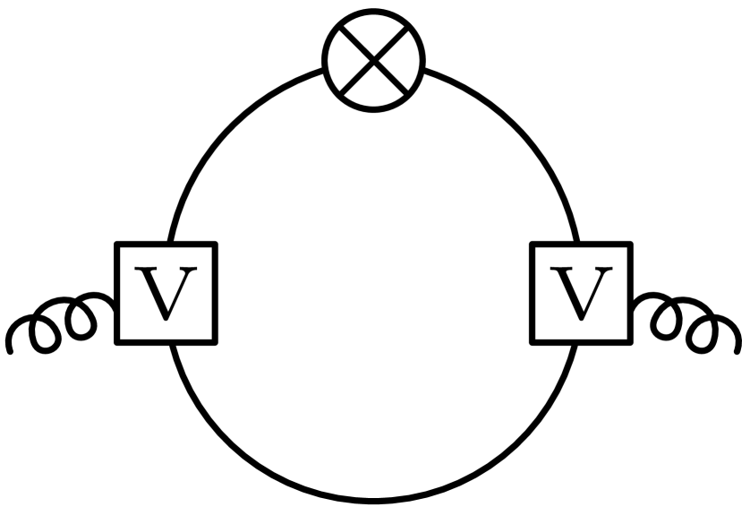
(a)

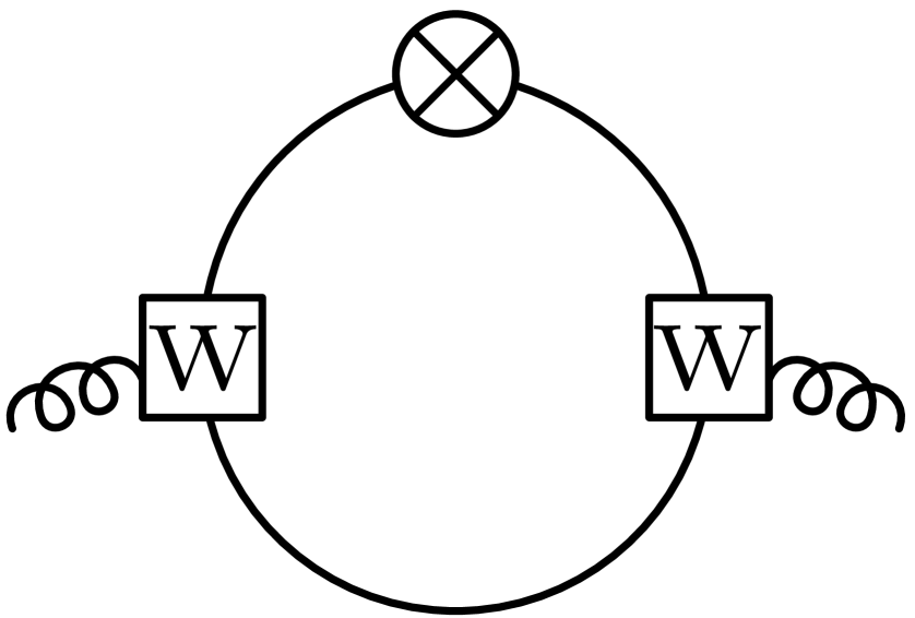
(b)

Figure 10: Diagrammatic representation of the contributions of the free Dirac Hamiltonian to the gluon gap equation, (a) eq. (94) and (b) eq. (95).

illustrated in fig. 10, and from the quark-gluon coupling in the Dirac Hamiltonian (9) resulting in the one-loop contributions

$$I_{V\mathrm{Q}}^{\mathrm{YM}}(k) =-2g^{2}\int\mathop{\mathrm{d}\mkern-7.0mu\mathchar 22\relax\mkern-1.0mu}\mkern-4.0mu^{3}p\,V(\boldsymbol{p},\boldsymbol{k}-\boldsymbol{p})X(\boldsymbol{p},\boldsymbol{k}-\boldsymbol{p})P(p)P(|\boldsymbol{k}-\boldsymbol{p}|)\left(1+S(p)S(|\boldsymbol{k}-\boldsymbol{p}|)\right)$$ (96)

$$I_{W\mathrm{Q}}^{\mathrm{YM}}(k) =-2g^{2}\int\mathop{\mathrm{d}\mkern-7.0mu\mathchar 22\relax\mkern-1.0mu}\mkern-4.0mu^{3}p\,W(\boldsymbol{p},\boldsymbol{k}-\boldsymbol{p})Y(\boldsymbol{p},\boldsymbol{k}-\boldsymbol{p})P(p)P(|\boldsymbol{k}-\boldsymbol{p}|)\left(S(p)+S(|\boldsymbol{k}-\boldsymbol{p}|)\right)$$ (97)

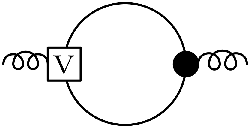
(a)

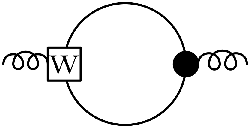
(b)

Figure 11: Diagrammatic representation of the contributions of the quark-gluon coupling in the Dirac Hamiltonian to the gluon gap equation, (a) eq. (96) and (b) eq. (97).

which are diagrammatically illustrated in fig. 11. Note that the quark contribution to the kinetic energy of the transversal gluons $\langle H_{\mathrm{YM}}^{E}\rangle$ [the last two terms in eq. (74)] does not contribute to the gluonic gap equation, while it does contribute to the quark gap equation (80).

Neglecting the quark-gluon coupling in the ansatz for the vacuum wave functional, $V=W=0$, the gluonic gap equation (90) agrees with the result from pure Yang–Mills theory, see eq. (91).

A fully unquenched calculation would now necessitate to solve the system of coupled integral equations for the scalar quark kernel $S$ and the bosonic kernel $\omega$, (80) and (90), while the vectorial kernels $V$ and $W$ can simply be expressed in terms of these two kernels, see (87) and (89). This goes beyond the scope of the present paper and will be subject of further research. Here we focus on the quark sector and confine ourselves mainly to a quenched calculation using the previously obtained results for the Yang–Mills sector as input. To be more precise, for the gluon energy $\omega$ we will use Gribov’s formula (29) which nicely fits the (quenched) lattice data. Furthermore, the true Coulomb potential (30) obtained in the variational approach Epple et al. (2007) can be approximated to good accuracy by the sum of a linearly rising potential and an ordinary Coulomb potential, which reads in momentum space

$$V_{\mathrm{C}}(p)=\frac{8\pi\sigma_{\mathrm{C}}}{p^{4}}-\frac{4\pi\alpha_{\mathrm{S}}}{p^{2}}=V_{\mathrm{C}}^{\mathrm{IR}}(p)+V_{\mathrm{C}}^{\mathrm{UV}}(p).$$ (98)

In accordance with lattice calculations we choose the Coulomb string tension as

$$\sigma_{\mathrm{C}}=2\sigma$$ (99)

with $\sigma=(440\,\mathrm{MeV})^{2}$ being the Wilson string tension.

VIII UV analysis and renormalization

In the quenched approximation only the quark gap equation for the scalar kernel $S$ remains to be solved while the vector kernels are explicitly available in terms of $\omega$ and $S$, see eqs. (87) and (89). The loop integrals in the quark gap equation contain UV divergences and the UV analysis carried out in appendix E reveals the following UV behavior: All loop integrals on the r.h.s. of the quark gap equation (80) contain linear and logarithmic UV divergences except for the one arising from the Coulomb term, $I_{\mathrm{C}}^{\mathrm{Q}}$ [eq. (81)], which is only logarithmically divergent. The logarithmic divergence arises here from the Coulomb potential $V_{\mathrm{C}}^{\mathrm{UV}}$, see eq. (98). The linear divergences are known to cancel by gauge invariance, at least in covariant perturbation theory. In fact, adding the linear divergent contributions in the quark gap equation (80) we find that they exactly cancel. To be more precise, this strict cancellation is a direct consequence of the inclusion of the vector kernel $W$ into the ansatz for the vacuum wave functional [eqs. (42) and (44)]. Without this kernel, the quark gap equation would contain both a logarithmic and a linear UV divergence, which makes the inclusion of $W$ not only a quantitative but also a qualitative improvement of the variational ansatz. Due to the strict cancellation of the linear UV divergences, the quark gap equation (80) contains only logarithmic divergences. The logarithmically divergent terms of the gap equation (80) sum up to

$$\frac{C_{\mathrm{F}}}{3\pi^{2}}g^{2}kS(k)\ln\frac{\Lambda}{\mu}$$ (100)

where $\Lambda$ is the UV cutoff and $\mu$ is an, so far, arbitrary momentum scale. As can be seen from this expression, the remaining logarithmic UV divergences are multiplied by a factor $g^{2}$ and can hence be absorbed in a renormalized coupling

$$\widetilde{g}^{2}(\mu)=g^{2}\ln\frac{\Lambda}{\mu}\,.$$ (101)

The renormalized coupling $\widetilde{g}$ is assumed to be finite so that the bare coupling $g$ vanishes for $\Lambda\to\infty$ like $1/\sqrt{\ln\Lambda}$. Ignoring terms which vanish for $\Lambda\to\infty$ with $\widetilde{g}^{2}(\mu)=\mathrm{const.}<\infty$ the renormalized quark gap equation reduces to

$$kS(k)\left[1-\frac{C_{\mathrm{F}}}{3\pi^{2}}\widetilde{g}^{2}(\mu)\right]=\frac{C_{\mathrm{F}}}{2}\int\mathop{\mathrm{d}\mkern-7.0mu\mathchar 22\relax\mkern-1.0mu}\mkern-4.0mu^{3}p\,V_{\mathrm{C}}^{\mathrm{IR}}(|\boldsymbol{p}-\boldsymbol{k}|)P(p)\left[S(p)\bigl{(}1-S^{2}(k)\bigr{)}-S(k)\bigl{(}1-S^{2}(p)\bigr{)}\hat{\boldsymbol{p}}\cdot\hat{\boldsymbol{k}}\right]\,.$$ (102)

This equation is considerably simpler than the unrenormalized gap equation (80). The whole effect of the quark gluon coupling as well as the UV part of the Coulomb potential $V_{\mathrm{C}}^{\mathrm{UV}}$ [eq. (98)] are now captured by the term multiplied by the renormalized coupling constant. In fact, the quark-gluon coupling and $V_{\mathrm{C}}^{\mathrm{UV}}$ equally contribute to the renormalized gap equation. When the renormalized coupling constant $\widetilde{g}$ is set to zero eq. (102) reduces to the gap equation of ref. Adler and Davis (1984).

If the confining part of the non-Abelian Coulomb potential is neglected, $V_{\mathrm{C}}^{\mathrm{IR}}=0$, the gap equation (102) has only the trivial solution $S=0$. This result is in agreement with the empirical findings of ref. Pak and Reinhardt (2013) that there is no spontaneous breaking of chiral symmetry when $V_{\mathrm{C}}^{\mathrm{IR}}$ is neglected. Although the quark-gluon coupling term alone cannot trigger spontaneous breaking of chiral symmetry it considerably increases the strength of the symmetry breaking as can be read off from eq. (102) and as will later on be confirmed by the numerical calculation. The r.h.s. of eq. (102) is independent of $\widetilde{g}$, while on the l.h.s. a non-zero $\widetilde{g}$ reduces the factor multiplying $kS(k)$ and thus increases $S$, which also increases the quark condensate (see below).

Renormalizing the static quark propagator (56) in the same way as the gap equation (80), see appendix E, we find for the renormalized propagator

$$G_{\mathrm{ren}}(\boldsymbol{p})=\frac{1}{2}\left[1-\frac{C_{\mathrm{F}}}{8\pi^{2}}\widetilde{g}^{2}(\mu)\right]P(p)\Bigl{[}\Bigl{(}1-S^{2}(p)\Bigr{)}\boldsymbol{\alpha}\cdot\hat{\boldsymbol{p}}+2S(p)\beta\Bigr{]}=\left[1-\frac{C_{\mathrm{F}}}{8\pi^{2}}\widetilde{g}^{2}(\mu)\right]\frac{\boldsymbol{\alpha}\cdot\boldsymbol{p}+\beta M(p)}{2\sqrt{p^{2}+M^{2}(p)}}\,.$$ (103)

Like the unrenormalized propagator (56) it has the quasi-particle form (62) with an effective (running) mass $M$ given by eq. (65) and the constant field renormalization factor

$$Z(p)=1-\frac{C_{\mathrm{F}}}{8\pi^{2}}\widetilde{g}^{2}(\mu)\,.$$ (104)

From the renormalized quark propagator (103) we find the renormalized quark condensate

$$\langle\bar{\psi}(\boldsymbol{x})\psi(\boldsymbol{x})\rangle=-4N_{\mathrm{C}}\left[1-\frac{C_{\mathrm{F}}}{8\pi^{2}}\widetilde{g}^{2}(\mu)\right]\int\mathop{\mathrm{d}\mkern-7.0mu\mathchar 22\relax\mkern-1.0mu}\mkern-4.0mu^{3}p\,P(p)S(p)\,.$$ (105)

Obviously, the quark condensate vanishes for the trivial solution $S=0$ of the gap equation. Furthermore, from the renormalized quark propagator (103) we can conclude that the (anti-)particle occupation numbers are given by

$$\langle{a_{\mathrm{ren}}^{s,m}}^{\dagger}(\boldsymbol{p})a_{\mathrm{ren}}^{s,m}(\boldsymbol{p})\rangle =P(p)S^{2}(p)$$ (106)

and

$$\left(1-\langle{b_{\mathrm{ren}}^{s,m}}^{\dagger}(\boldsymbol{p})b_{\mathrm{ren}}^{s,m}(\boldsymbol{p})\rangle\right) =P(p)\,,$$ (107)

respectively, where $a$ ($b$) is the annihilation operator for a (anti-)quark in momentum space, see appendix A. Note that we have, at this point, replaced the quark field $\psi$ in terms of the field renormalization factor $Z$ by the renormalized quantity $\psi_{\mathrm{ren}}$ in order to obtain the physical occupation numbers, i.e. $a_{\mathrm{ren}}^{\dagger}$, $b_{\mathrm{ren}}^{\dagger}$ generate properly normalized one-particle states. Furthermore, from eqs. (59), (106) and (107) one can read off immediately that $\langle a_{\mathrm{ren}}^{\dagger}a_{\mathrm{ren}}\rangle=\langle b_{\mathrm{ren}}^{\dagger}b_{\mathrm{ren}}\rangle$ holds.

The momentum scale $\mu$ introduced above in the context of the renormalized coupling (101) is completely arbitrary and can be chosen at will. However, in the quark gap equation (102) there is a physical scale inherited from the gluon sector: the Coulomb string tension $\sigma_{\mathrm{C}}$, see eq. (98). It is convenient to identify the arbitrary scale $\mu$ with $\sqrt{\sigma_{\mathrm{C}}}$. This choice of $\mu$ removes the Coulomb string tension from the gap equation when the latter is expressed in dimensionless variables. The only undetermined quantity in our variational equations of motion is then the renormalized coupling $\widetilde{g}$ at the scale $\mu=\sqrt{\sigma_{\mathrm{C}}}$.

IX Physical implications of the quark-gluon coupling

Below we investigate the immediate consequences of the quark-gluon coupling in our approach on both the quark and the gluon sector.

IX.1 Scaling properties of the quark sector

For the numerical solution of the gap equation (102) it is more convenient to express it in terms of the mass function $M$ [eq. (65)]. This yields

$$M(k)\left[1-\frac{C_{\mathrm{F}}}{3\pi^{2}}\widetilde{g}^{2}(\mu)\right]=4\pi C_{\mathrm{F}}\int\mathop{\mathrm{d}\mkern-7.0mu\mathchar 22\relax\mkern-1.0mu}\mkern-4.0mu^{3}p\,\frac{M(p)-M(k)\frac{\boldsymbol{p}\cdot\boldsymbol{k}}{{k}^{2}}}{|\boldsymbol{p}-\boldsymbol{k}|^{4}\sqrt{p^{2}+M^{2}(p)}}\,.$$ (108)

Note that the two-loop approximation breaks down when the renormalized coupling constant exceeds the critical value

$$\widetilde{g}_{\mathrm{c}}=\sqrt{\frac{3\pi^{2}}{C_{\mathrm{F}}}}=\sqrt{\frac{6\pi^{2}N_{\mathrm{C}}}{N_{\mathrm{C}}^{2}-1}}\,.$$ (109)

However, the critical values $\widetilde{g}_{\mathrm{c}}\approx 6.28$ for $SU(2)$ and $\widetilde{g}_{\mathrm{c}}\approx 4.71$ for $SU(3)$ are well above the value required to reproduce the phenomenological value of the quark condensate, see eq. (122) below, so that the collaps does not occur for realistic values of the renormalized coupling.

Denoting the IR limit of the mass function by $m=M(p=0)$ and the respective quantities for vanishing coupling by a superscript “0”, we find from the gap equation (108) the following, very useful scaling properties:

$$M(p)=\frac{m}{m^{0}}M^{0}(m^{0}p/m)\,,$$ (110)

where

$$m=\frac{m^{0}}{\sqrt{1-\frac{C_{\mathrm{F}}\widetilde{g}^{2}(\mu)}{3\pi^{2}}}}$$ (111)

holds. From these relations follows that it is sufficient to solve the gap equation (108) only for the case of a vanishing coupling $\widetilde{g}=0$ yielding the function $M^{0}$. The solution $M$ of eq. (108) for arbitrary coupling $\widetilde{g}$ is then obtained from the scaling relation (110). By means of this relation also the quark condensate $\langle\bar{\psi}\psi\rangle$ with quark-gluon coupling included can be related to that for $\widetilde{g}=0$, $\langle\bar{\psi}\psi\rangle^{0}$: Using eq. (65) to trade the scalar kernel $S$ in eq. (105) for the mass function $M$ and using subsequently the scaling relation (110) we find the following scaling relation for the quark condensate

$$\langle\bar{\psi}(\boldsymbol{x})\psi(\boldsymbol{x})\rangle=\frac{1-\frac{C_{\mathrm{F}}}{8\pi^{2}}\widetilde{g}^{2}(\mu)}{\sqrt{1-\frac{C_{\mathrm{F}}}{3\pi^{2}}\widetilde{g}^{2}(\mu)}^{3}}\langle\bar{\psi}(\boldsymbol{x})\psi(\boldsymbol{x})\rangle^{0}\,.$$ (112)

Inserting here for the renormalized quark-gluon coupling $\widetilde{g}$ at the scale $\mu=\sqrt{\sigma_{\mathrm{C}}}$ the value (122) determined in section X, we find the relation

$$\langle\bar{\psi}(\boldsymbol{x})\psi(\boldsymbol{x})\rangle=(1.42)^{3}\langle\bar{\psi}(\boldsymbol{x})\psi(\boldsymbol{x})\rangle^{0}$$ (113)

thus the quark-gluon coupling increases the quark condensate by $42\%$.

IX.2 Unquenching the gluon propagator

Below we solve the unquenched gluon gap equation (90) in a simplified way. This equation has the generic form

$$\omega^{2}(k)=\omega_{\mathrm{YM}}^{2}(k)+\omega_{\mathrm{Q}}^{2}(k)\,,$$ (114)

where $\omega_{\mathrm{YM}}$, defined by eq. (91), is the expression one finds from the pure Yang–Mills sector Feuchter and Reinhardt (2004a, b) and

$$\omega_{\mathrm{Q}}^{2}(k)=I_{VV}^{\mathrm{YM}}(k)+I_{WW}^{\mathrm{YM}}(k)+I_{V\mathrm{Q}}^{\mathrm{YM}}(k)+I_{W\mathrm{Q}}^{\mathrm{YM}}(k)$$ (115)

is the quark contribution, which consists of several one-loop terms defined by eqs. (94) to (97). Assuming for the scalar quark kernel $S$ a sufficiently fast vanishing UV asymptotics one can work out the UV behavior of these loop integrals (see appendix E) and finds that they are quadratic plus logarithmic divergent

$$\omega_{\mathrm{Q}}^{2}(k)=-\frac{g^{2}}{6\pi^{2}}\left[\Lambda^{2}-\frac{1}{2}\bigl{(}\omega^{2}(k)+k^{2}\bigr{)}\ln\frac{\Lambda}{\mu}\right]+\mbox{finite terms}\,.$$ (116)

The quadratic UV divergence is thus independent of the external momentum $k$. Such an UV divergence also occurs in the Yang–Mills sector, i.e. in $\omega_{\mathrm{YM}}$ (91) and can therefore be removed by the known renormalization procedure of the Yang–Mills sector, i.e. by the counterterm $\sim A^{2}$ Epple et al. (2008). Like in the quark gap equation, the (logarithmic) UV divergence is here multiplied by a factor $g^{2}$ and can be absorbed into the renormalized coupling constant $\widetilde{g}$ (101). Droping all terms which vanish for $\Lambda\to\infty$ for finite $\widetilde{g}$, we arrive at the unquenched renormalized gluon gap equation

$$\omega^{2}(k)=\bar{\omega}_{\mathrm{YM}}^{2}(k)+\frac{\widetilde{g}^{2}(\mu)}{12\pi^{2}}\bigl{(}\omega^{2}(k)+k^{2}\bigr{)}\,,$$ (117)

where $\bar{\omega}_{\mathrm{YM}}$ is the renormalized version of $\omega_{\mathrm{YM}}$ (91), see ref. Epple et al. (2008). The equation (117) can be solved for $\omega$ yielding

$$\omega^{2}(k)=\left[\frac{\widetilde{g}^{2}(\mu)}{12\pi^{2}}k^{2}+\bar{\omega}_{\mathrm{YM}}^{2}(k)\right]\left[1-\frac{\widetilde{g}^{2}(\mu)}{12\pi^{2}}\right]^{-1}.$$ (118)

To obtain a first estimate of the effect of unquenching on the gluon propagator we use for the quenched (renormalized) gluon energy $\bar{\omega}_{\mathrm{YM}}$ the Gribov formula (29). The resulting gluon propagator $1/(2\omega)$ is shown in fig. 12 together with the quenched Gribov propagator. The unquenching leads to a decrease of the gluon propagator in the mid-momentum regime but the effect of unquenching is small. A similar result was obtained in ref. Pak and Reinhardt (2013) where the unquenching was done in the same way.

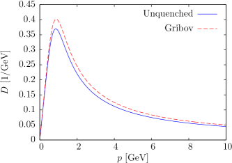
Figure 12: The static gluon propagator $D(p)=1/2\omega(p)$ as given by (118) for an effective coupling of $\widetilde{g}(\sqrt{\sigma_{\mathrm{C}}})=3.586$ (full line) and for the Gribov formula (dashed line).

X Numerical results

By the above derived scaling relation (110) we have reduced the numerical calculation to the case with vanishing quark-gluon coupling $\widetilde{g}=0$. The numerical solution of the remaining quark gap equation (108) (with $\widetilde{g}=0$) can be performed by standard methods, see e.g. ref. Watson and Reinhardt (2012). The resulting mass function for vanishing coupling can be nicely fitted by

$$M_{\mathrm{fit}}^{0}(p)=\frac{m^{0}}{1+ap^{2A}+2bp^{2B}}$$ (119)

with the optimized fit parameters

$$m^{0} =0.165508\, \quad\quad a =4.59935\, \quad\quad b =1.26155$$

$$A =0.985198\, \quad\quad B =2.27051\,.$$ (120)

From this fit we read-off the UV power-law behavior $M(p\to\infty)\sim p^{-4.54}$ which, according to (110), holds for arbitrary strengths of the quark-gluon coupling. This UV exponent differs somewhat from the value $(-4)$ found in refs. Watson and Reinhardt (2012); Pak and Reinhardt (2013) which, however, has almost no effect on the quantities calculated below since the UV part is highly suppressed.

We adjust the renormalized effective coupling constant $\widetilde{g}$ such that the phenomenological value

$$\langle\bar{\psi}(\boldsymbol{x})\psi(\boldsymbol{x})\rangle_{\mathrm{phen}}=(-235\,\mathrm{MeV})^{3}$$ (121)

is reproduced. This requires for $\sigma_{\mathrm{C}}=2\sigma$ an effective coupling constant of

$$\widetilde{g}(\sqrt{\sigma_{\mathrm{C}}})=3.586\,.$$ (122)

When the coupling of the quarks to the gluons is neglected one obtains (for the same value of the Coulomb string tension) for the quark condensate the substantially smaller value

$$\langle\bar{\psi}(\boldsymbol{x})\psi(\boldsymbol{x})\rangle^{0}=(-165\,\mathrm{MeV})^{3}\,.$$ (123)

Using for the renormalized coupling constant $\widetilde{g}$ the value (122) obtained from the phenomenological quark condensate one finds the solution of the gap equation (108) shown in fig. 13 (a). The IR mass is given by $m\approx 210\,\mathrm{MeV}$. For sake of comparison, fig. 13 (a) shows also the solution $M^{0}$ of the gap equation for vanishing quark-gluon coupling $\widetilde{g}=0$. The effective mass is then considerably smaller. This refers in particular to its IR value $m^{0}\approx 120\,\mathrm{MeV}$. Fig. 13 (b) shows the corresponding results for the scalar kernel $S$, which can be calculated from eq. (65) once $M$ is known. The IR value $S(p=0)=1$ is obtained independently of the value of the quark-gluon coupling constant $\widetilde{g}$ as one can also extract analytically from the gap equation. Neglecting the quark-gluon coupling considerably decreases $S$ in the mid-momentum regime. It is this momentum regime which dominantly contributes to the spontaneous breaking of chiral symmetry, i.e. to the quark condensate [see eq. (105)]. This is also found in lattice invesitgations Yamamoto and Suganuma (2010).

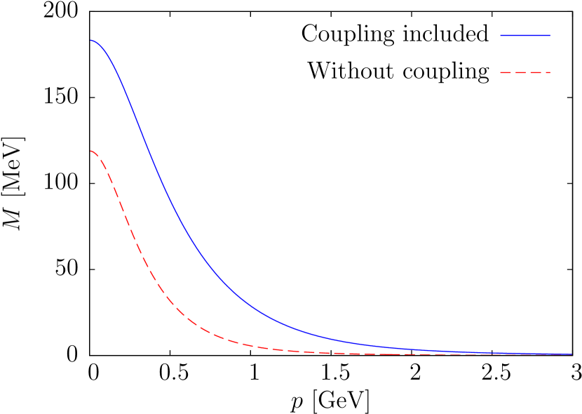
(a)

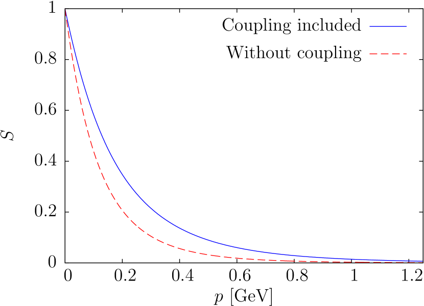
(b)

Figure 13: (a) Mass function for an effective coupling strength of $\widetilde{g}(\sqrt{\sigma_{\mathrm{C}}})=3.586$ (full curve) compared to the result obtained with a BCS-ansatz neglecting the coupling (dashed curve). The Coulomb string tension is set to $\sigma_{\mathrm{C}}=2\sigma$. (b) Scalar kernel for an effective coupling strength of $\widetilde{g}(\sqrt{\sigma_{\mathrm{C}}})=3.586$ (full curve) compared to the result neglecting the coupling (dashed curve).

With the scalar kernel $S$ at our disposal we are also able to determine the quark occupation number eq. (106). The resulting curve is shown in fig. 14. One can clearly observe that the inclusion of the quark-gluon coupling significantly increases the occupation number in the mid-momentum regime. Note that the same result holds for the occupation number of anti-quarks [see eq. (107) and the discussion following thereafter].

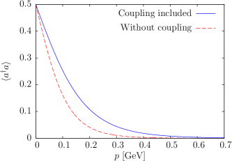
Figure 14: Occupation number of quarks according to eq. (106). The straight line shows the results for the quark-gluon coupling $\widetilde{g}(\sqrt{\sigma_{\mathrm{C}}})=3.586$ while the dashed one is for $\widetilde{g}=0$.

Finally, we explicitly evaluate the vector kernels $V$ [eq. (87)] and $W$ [eq. (89)] using the scalar kernel $S$ obtained above and the Gribov formula (29) as input for the gluon energy. The results are plotted in fig. 15 for the case that the moduli of the two momentum arguments agree. Although the shape of both form factors is similar they differ in the size (note the different scales used in figs. 15 (a) and (b), respectively): $V$ is considerably larger than $W$. Furthermore, for $p=q$ the kernel $W(\boldsymbol{p},\boldsymbol{q})$ drops off more rapidly in the UV ($p=q\to\infty$) than $V(\boldsymbol{p},\boldsymbol{q})$. This can be also read off from the explicit analytic expressions given in eqs. (87) and (89). From these expressions it also follows that $W$ is, in general, much more sensitive to the detailed behavior of the scalar kernel $S$ than $V$ (which is not surprising for $W$ being purely non-perturbative). Keeping one momentum argument, say $q$, fixed both vector form factors vanish like $1/p$ for $p\to\infty$.

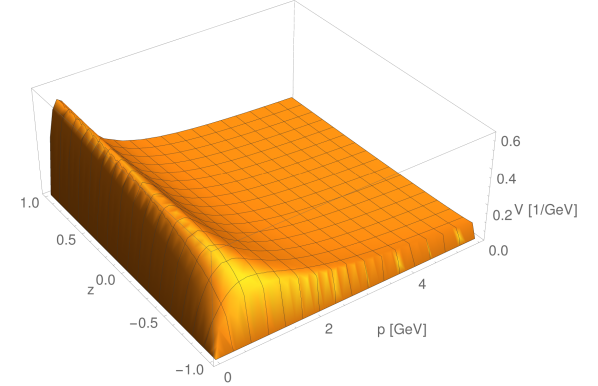
(a)

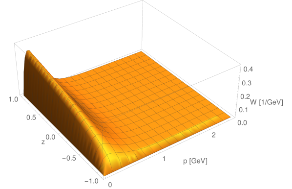
(b)

Figure 15: The vector kernels (a) $V(\boldsymbol{p},\boldsymbol{q})$ and (b) $W(\boldsymbol{p},\boldsymbol{q})$ for an effective coupling strength of $\widetilde{g}(\sqrt{\sigma_{\mathrm{C}}})=3.586$ as function of the modulus $p=q$ and $z=\cos\sphericalangle(\boldsymbol{p},\boldsymbol{q})$.

XI Summary and conclusions

In this paper the variational approach to QCD originally developed in refs. Feuchter and Reinhardt (2004a, b); Epple et al. (2007) for the Yang–Mills sector and extended in refs. Pak and Reinhardt (2012, 2013) to full QCD has been further developed and essentially improved in several regards: First we included the UV part $V_{\mathrm{C}}^{\mathrm{UV}}$ of the color Coulomb potential in the treatment of the quark sector which was not the case in refs. Pak and Reinhardt (2012, 2013). This additional contribution turns out to have the same effect on the renormalized gap equation as the quark-gluon coupling. Second, we have abandoned a simplifying approximation used in ref. Pak and Reinhardt (2013) and calculated the vacuum energy density consistently to two-loop order. The resulting expressions are consistent with the results obtained by using Dyson–Schwinger equations to carry out the variational approach Campagnari and Reinhardt (shed) and also with perturbation theory Campagnari and Reinhardt (2015b). Third, we have included an additional Dirac structure (with a new variational kernel) into the fermionic vacuum wave functional, thereby enlarging the space of trial states which improves the variational results. This new Dirac structure in the quark wave functional can be motivated by treating the quark-gluon coupling of the QCD Hamiltonian in perturbation theory on top of the non-trivial BCS-state obtained in a mean-field treatment of the non-Abelian Coulomb interaction. By including this new quark-gluon coupling term in the trial vacuum state all linear UV divergences are eliminated from the quark gap equation. The remaining logarithmic UV divergence has been absorbed into a renormalized coupling constant. In the resulting renormalized gap equation the total quark-gluon coupling becomes manifest in a rescaling of the effective (momentum dependent) quark mass. By using this scaling property physical quantities like the quark condensate can be related to their values when the quark-gluon coupling is switched off. In this way we could analytically show that the inclusion of the quark-gluon coupling in the vacuum wave functional leads to a substantial increase in the quark condensate and the effective quark mass. In our Hamiltonian approach to QCD in Coulomb gauge the quark sector inherits a scale from the gluon sector. This is given by the Coulomb string tension $\sigma_{\mathrm{C}}$, which also determines the Gribov mass $M_{\mathrm{G}}\approx\sigma_{\mathrm{C}}$. Choosing the renormalized coupling at this scale to reproduce the phenomenological value of the quark condensate, $\langle\bar{\psi}\psi\rangle=(-235\,\mathrm{MeV})^{3}$, requires a value of $\widetilde{g}(\sqrt{\sigma_{\mathrm{C}}})=3.586$.

Using for the quenched gluon propagator the lattice results, which can be nicely fitted by the Gribov formula, and renormalizing the full unquenched gluon gap equation consistently with the quark gap equation, we have shown that the unquenched gluon propagator is somewhat reduced in the mid-momentum regime compared to the quenched one but the effect is quite small.

The results obtained in the present paper are quite encouraging for further applications of the present approach. We plan to extend it to finite temperatures and baryon densities to study the deconfinement and chiral phase transitions. In a first application we will then calculate the quark contribution to the effective potential of the Polyakov loop extending the approach of ref. Reinhardt and Heffner (2013) to full QCD.

Appendix A Momentum representation

Due to translational invariance of the vacuum it is convenient to carry out the actual calculations in momentum space. Thereby, it will be convenient to expand the quark field $\psi$ in terms of the eigenspinors $u$, $v$ of the free Dirac Hamiltonian of chiral quarks

$$h_{0}(\boldsymbol{p})=\boldsymbol{\alpha}\cdot\boldsymbol{p}\,.$$ (124)

We choose the eigenspinors such that they satisfy the eigenvalue equation

$$\boldsymbol{\alpha}\cdot\boldsymbol{p}\,u^{s}(\boldsymbol{p})=pu^{s}(\boldsymbol{p}),\quad\quad\boldsymbol{\alpha}\cdot\boldsymbol{p}\,v^{s}(-\boldsymbol{p})=-pv^{s}(-\boldsymbol{p})$$ (125)

and are normalized according to

$${u^{s}}^{\dagger}(\boldsymbol{p})u^{t}(\boldsymbol{p}) ={v^{s}}^{\dagger}(-\boldsymbol{p})v^{t}(-\boldsymbol{p})=2p\delta^{st}$$ (126a)

$${u^{s}}^{\dagger}(\boldsymbol{p})v^{t}(-\boldsymbol{p}) ={v^{s}}^{\dagger}(-\boldsymbol{p})u^{t}(\boldsymbol{p})=0\,.$$ (126b)

Here $s=\pm 1$ denotes the double of the spin projection. The spinors satisfy the relations

$$\beta u^{s}(\boldsymbol{p}) =sv^{s}(-\boldsymbol{p})$$ (127a)

$$\beta v^{s}(-\boldsymbol{p}) =su^{s}(\boldsymbol{p})$$ (127b)

$$\gamma_{5}u^{s}(\boldsymbol{p}) =su^{s}(\boldsymbol{p})$$ (128a)

$$\gamma_{5}v^{s}(-\boldsymbol{p}) =-sv^{s}(-\boldsymbol{p})$$ (128b)

from which we can conclude

$$\bar{u}^{s}(\boldsymbol{p})u^{t}(\boldsymbol{p}) \equiv{u^{s}}^{\dagger}(\boldsymbol{p})\beta u^{t}(\boldsymbol{p})=0$$ (129a)

$$\bar{v}^{s}(-\boldsymbol{p})v^{t}(-\boldsymbol{p}) =0.$$ (129b)

For the outer product of the spinors one finds

$$u^{s}(\boldsymbol{p}){u^{s}}^{\dagger}(\boldsymbol{p}) =\frac{1}{2}p\bigl{(}\left[\mathbbm{1}+\boldsymbol{\alpha}\cdot\hat{\boldsymbol{p}}\right]+s\gamma_{5}\left[\mathbbm{1}+\boldsymbol{\alpha}\cdot\hat{\boldsymbol{p}}\right]\bigr{)}$$ (130a)

$$v^{s}(-\boldsymbol{p}){v^{s}}^{\dagger}(-\boldsymbol{p}) =\frac{1}{2}p\bigl{(}\left[\mathbbm{1}-\boldsymbol{\alpha}\cdot\hat{\boldsymbol{p}}\right]-s\gamma_{5}\left[\mathbbm{1}-\boldsymbol{\alpha}\cdot\hat{\boldsymbol{p}}\right]\bigr{)}$$ (130b)

$$u^{s}(\boldsymbol{p}){v^{s}}^{\dagger}(-\boldsymbol{p}) =\frac{1}{2}p\bigl{(}s\beta\left[\mathbbm{1}-\boldsymbol{\alpha}\cdot\hat{\boldsymbol{p}}\right]-\beta\gamma_{5}\left[\mathbbm{1}-\boldsymbol{\alpha}\cdot\hat{\boldsymbol{p}}\right]\bigr{)}$$ (130c)

$$v^{s}(-\boldsymbol{p}){u^{s}}^{\dagger}(\boldsymbol{p}) =\frac{1}{2}p\bigl{(}s\beta\left[\mathbbm{1}+\boldsymbol{\alpha}\cdot\hat{\boldsymbol{p}}\right]+\beta\gamma_{5}\left[\mathbbm{1}+\boldsymbol{\alpha}\cdot\hat{\boldsymbol{p}}\right]\bigr{)}$$ (130d)

while the matrix elements of the Dirac operator are given by

$${u^{s}}^{\dagger}(\boldsymbol{p})\boldsymbol{\alpha}\cdot\boldsymbol{q}u^{t}(\boldsymbol{p}) =2pq\bigl{(}\hat{\boldsymbol{p}}\cdot\hat{\boldsymbol{q}}\bigr{)}\delta^{st}$$ (131a)

$${v^{s}}^{\dagger}(-\boldsymbol{p})\boldsymbol{\alpha}\cdot\boldsymbol{q}v^{t}(-\boldsymbol{p}) =-2pq\bigl{(}\hat{\boldsymbol{p}}\cdot\hat{\boldsymbol{q}}\bigr{)}\delta^{st}$$ (131b)

$${u^{s}}^{\dagger}(\boldsymbol{p})\boldsymbol{\alpha}\cdot\boldsymbol{q}v^{s}(-\boldsymbol{p}) =0$$ (131c)

$${v^{s}}^{\dagger}(-\boldsymbol{p})\boldsymbol{\alpha}\cdot\boldsymbol{q}u^{s}(\boldsymbol{p}) =0\,.$$ (131d)

In terms of these eigenspinors the quark field can be expanded as

$$\psi^{m}(\boldsymbol{x})=\int\mathop{\mathrm{d}\mkern-7.0mu\mathchar 22\relax\mkern-1.0mu}\mkern-4.0mu^{3}p\,\frac{1}{\sqrt{2p}}\exp(\mathrm{i}\boldsymbol{p}\cdot\boldsymbol{x})\Bigl{(}a^{s,m}(\boldsymbol{p})u^{s}(\boldsymbol{p})+{b^{s,m}}^{\dagger}(-\boldsymbol{p})v^{s}(-\boldsymbol{p})\Bigr{)}$$ (132)

where $a^{s}$ ($b^{s}$) is the annihilation operator of a (anti-)quark in a state with spin projection $s/2=\pm 1/2$. With the normalization (126) of the eigenspinors the fermionic anti-commutation relations (10) are fulfilled when the $a,b$ satisfy the relations

$$\left\{a^{s,m}(\boldsymbol{p}),{a^{t,n}}^{\dagger}(\boldsymbol{q})\right\}=\left\{b^{s,m}(\boldsymbol{p}),{b^{t,n}}^{\dagger}(\boldsymbol{q})\right\}=\delta^{st}\delta^{mn}\delta\mkern-8.0mu\mathchar 22\relax^{3}(\boldsymbol{p}-\boldsymbol{q})$$ (133)

with all other anti-commutators vanishing. With the expansion (132) and the orthonormality relation of the Dirac eigenmodes our quark vacuum wave functional (42) aquires the form

$$\rvert\phi_{\mathrm{Q}}[A]\rangle=\exp\left(-\int\mathop{\mathrm{d}\mkern-7.0mu\mathchar 22\relax\mkern-1.0mu}\mkern-4.0mu^{3}p\int\mathop{\mathrm{d}\mkern-7.0mu\mathchar 22\relax\mkern-1.0mu}\mkern-4.0mu^{3}q\,K^{st,mn}(\boldsymbol{p},\boldsymbol{q}){a^{s,m}}^{\dagger}(\boldsymbol{p}){b^{t,n}}^{\dagger}(\boldsymbol{q})\right)\rvert 0\rangle$$ (134)

where the kernel $K$ in momentum space is related to that in the coordinate representation by

$$K^{st,mn}(\boldsymbol{p},\boldsymbol{q}) =\frac{1}{2\sqrt{pq}}{u^{s}}^{\dagger}(\boldsymbol{p})\int\mathrm{d}^{3}x\int\mathrm{d}^{3}y\,\exp\bigl{(}-\mathrm{i}\boldsymbol{p}\cdot\boldsymbol{x}-\mathrm{i}\boldsymbol{q}\cdot\boldsymbol{y}\bigr{)}K^{mn}(\boldsymbol{x},\boldsymbol{y})v^{t}(\boldsymbol{q})$$

$$=\delta^{mn}\delta^{st}\delta\mkern-8.0mu\mathchar 22\relax(\boldsymbol{p}+\boldsymbol{q})sS(p)+g\frac{1}{2\sqrt{pq}}t_{mn}^{a}{u^{s}}^{\dagger}(\boldsymbol{p})\bigl{(}V(\boldsymbol{p},\boldsymbol{q})+\beta W(\boldsymbol{p},\boldsymbol{q})\bigr{)}\alpha_{k}v^{t}(\boldsymbol{q})A_{k}^{a}(\boldsymbol{p}+\boldsymbol{q})\,.$$ (135)

The Fourier transforms of the variational kernels $S$, $V$ and $W$ contained in our trial ansatz (44) are hereby given by

$$S(p) =\int\mathrm{d}^{3}x\,\exp(-\mathrm{i}\boldsymbol{p}\cdot\boldsymbol{x})S(x)$$ (136)

$$V(\boldsymbol{p},\boldsymbol{q}) =\int\mathrm{d}^{3}x\int\mathrm{d}^{3}y\,\exp(-\mathrm{i}\boldsymbol{p}\cdot\boldsymbol{x}-\mathrm{i}\boldsymbol{q}\cdot\boldsymbol{y})V(\boldsymbol{x}+\boldsymbol{z},\boldsymbol{y}+\boldsymbol{z};\boldsymbol{z})$$ (137)

$$W(\boldsymbol{p},\boldsymbol{q}) =\int\mathrm{d}^{3}x\int\mathrm{d}^{3}y\,\exp(-\mathrm{i}\boldsymbol{p}\cdot\boldsymbol{x}-\mathrm{i}\boldsymbol{q}\cdot\boldsymbol{y})W(\boldsymbol{x}+\boldsymbol{z},\boldsymbol{y}+\boldsymbol{z};\boldsymbol{z})$$ (138)

and are assumed to be scalar functions. In order to obey the correct behavior under spatial transformations, these kernels have to fulfill the relations $S(\boldsymbol{p})=S(p)$, $V(\boldsymbol{p},\boldsymbol{q})=V(-\boldsymbol{p},-\boldsymbol{q})$ and $W(\boldsymbol{p},\boldsymbol{q})=W(-\boldsymbol{p},-\boldsymbol{q})$, respectively. Note that contrary to the scalar kernel $S$, the vector kernels $V$ and $W$ have dimension of inverse momentum. In order to simplify our calculations, we will assume all kernels to be real valued functions and the vector kernels additionally to be symmetric, i.e. $V(\boldsymbol{p},\boldsymbol{q})=V(\boldsymbol{q},\boldsymbol{p})$ and $W(\boldsymbol{p},\boldsymbol{q})=W(\boldsymbol{q},\boldsymbol{p})$, respectively.

Appendix B Perturbative motivation of the ansatz for the fermionic vacuum state

In Campagnari and Reinhardt (2015b), QCD in Coulomb gauge was treated in Rayleigh–Schrödinger perturbation theory up to order $g^{2}$ in the coupling and the known results of covariant perturbation theory were reproduced. The perturbative results of ref. Campagnari and Reinhardt (2015b) yield a quark vacuum wave functional of the form of our ansatz (42) and (44), however, with $S=0$ and $W=0$. The result obtained for the vector kernel $V$ agrees with the UV limit (88) of our variational result (87) as one expects due to asymptotic freedom. However, perturbation theory does not produce non-vanishing scalar and vector form factors, $S$ and $W$. As we have seen in the body of the paper both form factors are non-perturbative features. In particular, the variational result (89) for $W$ disappears in the chirally symmetric phase $S=0$. In order to get information on the kinematic structure of the vector form factor $W$ we treat the quark-gluon coupling in Rayleigh–Schrödinger perturbation theory using, however, as unperturbed quark vacuum wave functional not the bare (perturbative) vacuum $|0\rangle$ but the BCS-state $|0\rangle_{\mathrm{BCS}}$ given by eq. (42) with $V=W=0$ and $S\neq 0$ determined from the gap equation (102) with $\widetilde{g}=0$. In this sense the BCS-wave functional represents an approximate solution of the functional Schrödinger equation for the Hamiltonian

$$\bar{H}^{\prime}_{\mathrm{Q}}\equiv H_{\mathrm{Q}}^{0}+H_{\mathrm{C}}^{\mathrm{Q}}$$ (139)

in the mean-field approximation. What is left out in $\bar{H}^{\prime}_{\mathrm{Q}}$ is the quark-gluon coupling $H_{\mathrm{Q}}^{A}$,

$$\bar{H}_{\mathrm{Q}}=\bar{H}^{\prime}_{\mathrm{Q}}+H_{\mathrm{Q}}^{A}\,,$$ (140)

whose effect we will now study in perturbation theory on top of the BCS-ground state $|\phi_{\mathrm{Q}}[A=0]\rangle\equiv|0\rangle_{\mathrm{BCS}}$ which is in momentum space given by

$$|0\rangle_{\mathrm{BCS}}=\exp\left(-s\int\mathop{\mathrm{d}\mkern-7.0mu\mathchar 22\relax\mkern-1.0mu}\mkern-4.0mu^{3}p\,S(p){a^{s,m}}^{\dagger}(\boldsymbol{p}){b^{s,m}}^{\dagger}(-\boldsymbol{p})\right)|0\rangle\,,$$ (141)

see eqs. (134) and (135). Therefore, the “bare” QCD vacuum state which we consider now as starting point for perturbation theory reads $|0\rangle_{\mathrm{QCD}}=|0\rangle_{\mathrm{YM}}\otimes|0\rangle_{\mathrm{BCS}}$ where the bosonic part $|0\rangle_{\mathrm{YM}}$ is chosen similar to ref. Campagnari and Reinhardt (2015b), i.e. by eq. (46) with $\omega(p)$ replaced by the photon energy $p$. The perturbative vacuum state is hence given by

$$|0\rangle_{\mathrm{pert}}\sim|0\rangle_{\mathrm{QCD}}+g|0\rangle_{\mathrm{QCD}}^{1}+g^{2}|0\rangle_{\mathrm{QCD}}^{2}+\mathcal{O}(g^{3})$$ (142)

with the corrections $|0\rangle_{\mathrm{QCD}}^{i}$ being orthogonal to the unperturbed state $|0\rangle_{\mathrm{QCD}}$,

$${}_{\mathrm{QCD}}\langle 0|0\rangle_{\mathrm{QCD}}^{i}=0\quad\forall i\,.$$ (143)

Rewriting the gauge fixed QCD Hamiltonian (1) as a series in powers of the coupling $g$,

$$H_{\mathrm{QCD}}=H_{0}+gH_{1}+g^{2}H_{2}+\mathcal{O}(g^{3})\,,$$ (144)

the (first order) perturbative corrections to the vacuum $|0\rangle_{\mathrm{QCD}}$ is given by

$$|0\rangle_{\mathrm{QCD}}^{1}=-\sum_{N}\frac{\langle N|H_{1}|0\rangle_{\mathrm{QCD}}}{E_{N}-E_{0}}|N\rangle$$ (145)

with $|N\rangle$ denoting a $N$-particle state with energy $E_{N}$ and $E_{0}$ being the (bare) vacuum energy. Note that the bare vacuum is not an eigenstate of the bare Hamiltonian $H_{0}$ (this would be given by $|0\rangle_{\mathrm{YM}}\otimes|0\rangle$) but of the mean field Hamiltonian given by the sum of $H_{0}$ and the (fermionic) effective single particle part of $H_{2}$ (the fermionic part of $g^{2}H_{2}$ represents the Coulomb term $H_{\mathrm{C}}^{\mathrm{Q}}$ (17)), as can be seen explicitly after performing a Bogoljubov transformation. In the quark sector, (145) gives the only relevant correction to the BCS-wave functional since the relevant contribution from $H_{2}$ is already included in the choice of the fermionic vacuum, eq. (141). The first order correction $H_{1}$ to the unperturbed Hamiltonian is given by the quark-gluon coupling

$$H_{1}=\int\mathrm{d}^{3}x\,\psi^{\dagger}(\boldsymbol{x})\boldsymbol{\alpha}\cdot\boldsymbol{A}^{a}(\boldsymbol{x})t^{a}\psi(\boldsymbol{x})\,.$$ (146)

Inserting the expansion (132) for the quark fields into (146), we find that the only non-vanishing contribution to the correction (145) comes from states containing one gluon, one quark and one anti-quark, i.e.

$$|N\rangle\sim A_{k}^{a}(-\boldsymbol{p}_{1}){a^{s,m}}^{\dagger}(\boldsymbol{p}_{2}){b^{t,n}}^{\dagger}(\boldsymbol{p}_{3})|0\rangle_{\mathrm{QCD}}.$$ (147)

With this wave function we can easily calculate the matrix element in the numerator of (145) yielding

$$\langle N|H_{1}|0\rangle_{\mathrm{QCD}} \sim-t_{mn}^{a}t_{kl}(\boldsymbol{p}_{1})\frac{1}{2p_{1}}\delta\mkern-8.0mu\mathchar 22\relax(\boldsymbol{p}_{1}+\boldsymbol{p}_{2}+\boldsymbol{p}_{3})\frac{1}{2\sqrt{p_{2}p_{3}}}P(p_{2})P(p_{3})$$

$$\phantom{\sim}\,\,\quad\times{u^{s}}^{\dagger}(\boldsymbol{p}_{2})\Bigl{(}\bigl{[}1+S(p_{2})S(p_{3})\bigr{]}\alpha_{l}+\bigl{[}S(p_{2})+S(p_{3})\bigr{]}\beta\alpha_{l}\Bigr{)}v^{t}(\boldsymbol{p}_{3})$$ (148)

where $t_{kl}(\boldsymbol{p})=\delta_{kl}-\hat{\boldsymbol{p}}_{k}\hat{\boldsymbol{p}}_{l}$ is the transversal projector in momentum space. From eq. (148) we can already read-off the (Dirac) structure of the corrections to the bare vacuum. Inserting (148) together with (147) into (145) we find for the fermionic part of the (perturbative) wave functional

$$|0\rangle_{\mathrm{pert}}^{\mathrm{Q}}\sim\left(1+g\int\mathrm{d}^{3}x\int\mathrm{d}^{3}y\int\mathrm{d}^{3}z\,\psi_{+}^{\dagger}(\boldsymbol{x})\Bigl{[}f(\boldsymbol{x},\boldsymbol{y};\boldsymbol{z})+g(\boldsymbol{x},\boldsymbol{y};\boldsymbol{z})\beta\Bigr{]}\boldsymbol{\alpha}\cdot\boldsymbol{A}^{a}(\boldsymbol{z})t^{a}\psi_{-}(\boldsymbol{y})\right)|0\rangle_{\mathrm{BCS}}$$ (149)

where we have switched to the coordinate space representation for sake of comparison with our ansatz (42). Equation (149) exhibits precisely the (Dirac) structure of the quark-gluon coupling assumed in our ansatz (42) for the vacuum wave functional. Let us also mention that the $S$-dependence of the numerator of (148) perfectly agrees with the one obtained for the vector kernels from the variational principle, see eqs. (87) and (89). Note, furthermore, that the results obtained here reduce to the ones of ref. Campagnari and Reinhardt (2015b) when the limit $S\to 0$ is considered. Particularly, the additional term with the Dirac structure $\beta\alpha_{i}$ vanishes in this limit and can therefore not be recovered in perturbation theory starting from the bare fermionic vacuum $|0\rangle$.

Appendix C Explicit calculation of the static quark propagator

Using the fermionic anticommutator (10) and the expansion (132) of the quark field, the static quark propagator (51) can be expressed as

$$G_{ij}^{m_{1}m_{2}}(\boldsymbol{x},\boldsymbol{y})+\frac{1}{2}\delta^{m_{1}m_{2}}\delta_{ij}\delta(\boldsymbol{x}-\boldsymbol{y})=\langle\psi_{i}^{m_{1}}(\boldsymbol{x}){\psi_{j}^{m_{2}}}^{\dagger}(\boldsymbol{y})\rangle=$$

$$\quad=\int\mathop{\mathrm{d}\mkern-7.0mu\mathchar 22\relax\mkern-1.0mu}\mkern-4.0mu^{3}p_{1}\int\mathop{\mathrm{d}\mkern-7.0mu\mathchar 22\relax\mkern-1.0mu}\mkern-4.0mu^{3}p_{2}\,\frac{1}{2\sqrt{p_{1}p_{2}}}\Bigl{(}\langle a^{s_{1},m_{1}}(\boldsymbol{p}_{1}){a^{s_{2},m_{2}}}^{\dagger}(\boldsymbol{p}_{2})\rangle u_{i}^{s_{1}}(\boldsymbol{p}_{1}){u_{j}^{s_{2}}}^{\dagger}(\boldsymbol{p}_{2})\exp\bigl{(}\mathrm{i}\boldsymbol{p}_{1}\cdot\boldsymbol{x}-\mathrm{i}\boldsymbol{p}_{2}\cdot\boldsymbol{y}\bigr{)}$$

$$\quad\phantom{=}\,\,\phantom{\int\mathop{\mathrm{d}\mkern-7.0mu\mathchar 22\relax\mkern-1.0mu}\mkern-4.0mu^{3}p_{1}\int\mathop{\mathrm{d}\mkern-7.0mu\mathchar 22\relax\mkern-1.0mu}\mkern-4.0mu^{3}p_{2}\,\frac{1}{2\sqrt{p_{1}p_{2}}}\Bigl{(}}+\langle a^{s_{1},m_{1}}(\boldsymbol{p}_{1})b^{s_{2},m_{2}}(\boldsymbol{p}_{2})\rangle u_{i}^{s_{1}}(\boldsymbol{p}_{1}){v_{j}^{s_{2}}}^{\dagger}(\boldsymbol{p}_{2})\exp\bigl{(}\mathrm{i}\boldsymbol{p}_{1}\cdot\boldsymbol{x}+\mathrm{i}\boldsymbol{p}_{2}\cdot\boldsymbol{y}\bigr{)}$$

$$\quad\phantom{=}\,\,\phantom{\int\mathop{\mathrm{d}\mkern-7.0mu\mathchar 22\relax\mkern-1.0mu}\mkern-4.0mu^{3}p_{1}\int\mathop{\mathrm{d}\mkern-7.0mu\mathchar 22\relax\mkern-1.0mu}\mkern-4.0mu^{3}p_{2}\,\frac{1}{2\sqrt{p_{1}p_{2}}}\Bigl{(}}+\langle{b^{s_{1},m_{1}}}^{\dagger}(\boldsymbol{p}_{1}){a^{s_{2},m_{2}}}^{\dagger}(\boldsymbol{p}_{2})\rangle v_{i}^{s_{1}}(\boldsymbol{p}_{1}){u_{j}^{s_{2}}}^{\dagger}(\boldsymbol{p}_{2})\exp\bigl{(}-\mathrm{i}\boldsymbol{p}_{1}\cdot\boldsymbol{x}-\mathrm{i}\boldsymbol{p}_{2}\cdot\boldsymbol{y}\bigr{)}$$

$$\quad\phantom{=}\,\,\phantom{\int\mathop{\mathrm{d}\mkern-7.0mu\mathchar 22\relax\mkern-1.0mu}\mkern-4.0mu^{3}p_{1}\int\mathop{\mathrm{d}\mkern-7.0mu\mathchar 22\relax\mkern-1.0mu}\mkern-4.0mu^{3}p_{2}\,\frac{1}{2\sqrt{p_{1}p_{2}}}\Bigl{(}}+\langle{b^{s_{1},m_{1}}}^{\dagger}(\boldsymbol{p}_{1})b^{s_{2},m_{2}}(\boldsymbol{p}_{2})\rangle v_{i}^{s_{1}}(\boldsymbol{p}_{1}){v_{j}^{s_{2}}}^{\dagger}(\boldsymbol{p}_{2})\exp\bigl{(}-\mathrm{i}\boldsymbol{p}_{1}\cdot\boldsymbol{x}+\mathrm{i}\boldsymbol{p}_{2}\cdot\boldsymbol{y}\bigr{)}\Bigr{)}\,.$$ (150)

The fermionic expectation values of the quark two-point functions were given in eq. (52) in coordinate space. After Fourier transformation one finds e.g.

$$\langle a^{s_{1},m_{1}}(\boldsymbol{p}_{1}){a^{s_{2},m_{2}}}^{\dagger}(\boldsymbol{p}_{2})\rangle_{\mathrm{Q}}={\left[\mathbbm{1}+KK^{\dagger}\right]^{-1}}^{s_{1}s_{2},m_{1}m_{2}}(\boldsymbol{p}_{1},\boldsymbol{p}_{2})\,.$$ (151)

The bosonic expectation value of this quantity is taken by using eq. (54),

$$\langle a^{s_{1},m_{1}}(\boldsymbol{p}_{1}){a^{s_{2},m_{2}}}^{\dagger}(\boldsymbol{p}_{2})\rangle ={\left[\mathbbm{1}+KK^{\dagger}\right]^{-1}}^{s_{1}s_{2},m_{1}m_{2}}(\boldsymbol{p}_{1},\boldsymbol{p}_{2})\Bigr{|}_{A=0}$$

$$\phantom{=}\,\,+\frac{1}{4}\int\mathop{\mathrm{d}\mkern-7.0mu\mathchar 22\relax\mkern-1.0mu}\mkern-4.0mu^{3}q\,\frac{\delta}{\delta A_{k}^{a}(\boldsymbol{q})}t_{kl}(\boldsymbol{q})\frac{1}{\omega(q)}\frac{\delta}{\delta A_{l}^{a}(-\boldsymbol{q})}{\left[\mathbbm{1}+KK^{\dagger}\right]^{-1}}^{s_{1}s_{2},m_{1}m_{2}}(\boldsymbol{p}_{1},\boldsymbol{p}_{2})\Bigr{|}_{A=0}\,.$$ (152)

With

$$(KK^{\dagger})^{s_{1}s_{2},m_{1}m_{2}}(\boldsymbol{p}_{1},\boldsymbol{p}_{2})\Bigr{|}_{A=0}=\delta^{s_{1}s_{2}}\delta^{m_{1}m_{2}}\delta\mkern-8.0mu\mathchar 22\relax^{3}(\boldsymbol{p}_{1}-\boldsymbol{p}_{2})S^{2}(p_{1})\,,$$ (153)

we find for the leading order contribution

$${\left[\mathbbm{1}+KK^{\dagger}\right]^{-1}}^{s_{1}s_{2},m_{1}m_{2}}(\boldsymbol{p}_{1},\boldsymbol{p}_{2})\Bigr{|}_{A=0}=\delta^{s_{1}s_{2}}\delta^{m_{1}m_{2}}\delta\mkern-8.0mu\mathchar 22\relax^{3}(\boldsymbol{p}_{1}-\boldsymbol{p}_{2})P(p_{1})\,.$$ (154)

For the next to leading order contribution, we obtain after a short calculation

$$\frac{\delta}{\delta A_{k}^{a}(\boldsymbol{q})}\frac{\delta}{\delta A_{l}^{a}(-\boldsymbol{q})}{\left[\mathbbm{1}+KK^{\dagger}\right]^{-1}}^{s_{1}s_{2},m_{1}m_{2}}(\boldsymbol{p}_{1},\boldsymbol{p}_{2})\Bigr{|}_{A=0}=$$

$$\quad=P(p_{1})P(p_{2})\int\mathop{\mathrm{d}\mkern-7.0mu\mathchar 22\relax\mkern-1.0mu}\mkern-4.0mu^{3}p_{3}\,P(p_{3})\left.\frac{\delta(KK^{\dagger})^{s_{1}s_{3},m_{1}m_{3}}(\boldsymbol{p}_{1},\boldsymbol{p}_{3})}{\delta A_{k}^{a}(\boldsymbol{q})}\frac{\delta(KK^{\dagger})^{s_{3}s_{2},m_{3}m_{2}}(\boldsymbol{p}_{3},\boldsymbol{p}_{2})}{\delta A_{l}^{a}(-\boldsymbol{q})}\right|_{A=0}$$

$$\quad\phantom{=}\,\,+P(p_{1})P(p_{2})\int\mathop{\mathrm{d}\mkern-7.0mu\mathchar 22\relax\mkern-1.0mu}\mkern-4.0mu^{3}p_{3}\,P(p_{3})\left.\frac{\delta(KK^{\dagger})^{s_{1}s_{3},m_{1}m_{3}}(\boldsymbol{p}_{1},\boldsymbol{p}_{3})}{\delta A_{l}^{a}(-\boldsymbol{q})}\frac{\delta(KK^{\dagger})^{s_{3}s_{2},m_{3}m_{2}}(\boldsymbol{p}_{3},\boldsymbol{p}_{2})}{\delta A_{k}^{a}(\boldsymbol{q})}\right|_{A=0}$$

$$\quad\phantom{=}\,\,-P(p_{1})P(p_{2})\frac{\delta^{2}(KK^{\dagger})^{s_{1}s_{2},m_{1}m_{2}}(\boldsymbol{p}_{1},\boldsymbol{p}_{2})}{\delta A_{k}^{a}(\boldsymbol{q})\delta A_{l}^{a}(-\boldsymbol{q})}\,.$$ (155)

Inserting here for the variational kernel the explicit form (135) and carrying out the functional derivatives $\delta/\delta A$ the Dirac and color structure of these expressions can be worked out using the relations of appendix A. One finds eventually

$$\langle a^{s_{1},m_{1}}(\boldsymbol{p}_{1}){a^{s_{2},m_{2}}}^{\dagger}(\boldsymbol{p}_{2})\rangle=\delta^{s_{1}s_{2}}\delta^{m_{1}m_{2}}\delta\mkern-8.0mu\mathchar 22\relax^{3}(\boldsymbol{p}_{1}-\boldsymbol{p}_{2})P(p_{1})\left[1-\frac{1}{2}I_{\alpha}(\boldsymbol{p}_{1})\right]$$ (156)

where $I_{\alpha}$ is defined in eq. (57). Inserting now eq. (156) back into eq. (150) eventually enables us to calculate the outer product $uu^{\dagger}$ of the eigenspinors yielding an expression given in terms of Dirac matrices, see appendix A. Performing a similar calculation for the remaining two-point functions in (150) yields finally the expression given in eq. (56).

Appendix D Ground state energy revisited

D.1 Expectation value of the free Dirac Hamiltonian

Inserting the explicit expression for the quark propagator (56) into eq. (68) and taking the trace yields the following expression for the expectation value of the free Dirac Hamiltonian:

$$\langle H_{\mathrm{Q}}^{0}\rangle =2N_{\mathrm{C}}\delta\mkern-8.0mu\mathchar 22\relax^{3}(0)\int\mathop{\mathrm{d}\mkern-7.0mu\mathchar 22\relax\mkern-1.0mu}\mkern-4.0mu^{3}p\,p\bigl{(}1-2P(p)\bigr{)}$$

$$\phantom{=}\,\,+\frac{N_{\mathrm{C}}^{2}-1}{2}\delta\mkern-8.0mu\mathchar 22\relax^{3}(0)g^{2}\int\mathop{\mathrm{d}\mkern-7.0mu\mathchar 22\relax\mkern-1.0mu}\mkern-4.0mu^{3}p\int\mathop{\mathrm{d}\mkern-7.0mu\mathchar 22\relax\mkern-1.0mu}\mkern-4.0mu^{3}q\,\frac{V^{2}(\boldsymbol{p},\boldsymbol{q})}{\omega(|\boldsymbol{p}+\boldsymbol{q}|)}P(p)P(q)X(\boldsymbol{p},\boldsymbol{q})$$

$$\phantom{=}\,\,\quad\quad\times\Bigl{[}pP(p)\bigl{(}1-S^{2}(p)+2S(p)S(q)\bigr{)}+qP(q)\bigl{(}1-S^{2}(q)+2S(p)S(q)\bigr{)}\Bigr{]}$$

$$\phantom{=}\,\,+\frac{N_{\mathrm{C}}^{2}-1}{2}\delta\mkern-8.0mu\mathchar 22\relax^{3}(0)g^{2}\int\mathop{\mathrm{d}\mkern-7.0mu\mathchar 22\relax\mkern-1.0mu}\mkern-4.0mu^{3}p\int\mathop{\mathrm{d}\mkern-7.0mu\mathchar 22\relax\mkern-1.0mu}\mkern-4.0mu^{3}q\,\frac{W^{2}(\boldsymbol{p},\boldsymbol{q})}{\omega(|\boldsymbol{p}+\boldsymbol{q}|)}P(p)P(q)Y(\boldsymbol{p},\boldsymbol{q})$$

$$\phantom{=}\,\,\quad\quad\times\Bigl{[}pP(p)\bigl{(}1-S^{2}(p)-2S(p)S(q)\bigr{)}+qP(q)\bigl{(}1-S^{2}(q)-2S(p)S(q)\bigr{)}\Bigr{]}$$ (157)

D.2 Expectation value of the kinetic energy

In order to calculate the expectation value of $\widetilde{H}_{\mathrm{YM}}^{E}$ (73), we consider first those terms of $\widetilde{H}_{\mathrm{YM}}^{E}$ which explicitly contain the Faddeev–Popov determinant $J$. Using the approximation (27), the functional derivatives induced by the canonical momentum operator $\Pi$ can be easily carried out yielding expressions whose fermionic expectation value is trivial while the bosonic one can be calculated in terms of Wick’s theorem (50) leading to the result

$$-\frac{1}{8}\Bigl{\langle}\int\mathop{\mathrm{d}\mkern-7.0mu\mathchar 22\relax\mkern-1.0mu}\mkern-4.0mu^{3}p\,\bigl{[}\Pi_{k}^{a}(\boldsymbol{p})\ln J\bigr{]}\bigl{[}\Pi_{k}^{a}(-\boldsymbol{p})\ln J\bigr{]}\Bigr{\rangle} =\frac{N_{\mathrm{C}}^{2}-1}{2}\delta\mkern-8.0mu\mathchar 22\relax^{3}(0)\int\mathop{\mathrm{d}\mkern-7.0mu\mathchar 22\relax\mkern-1.0mu}\mkern-4.0mu^{3}p\,\frac{\chi^{2}(p)}{\omega(p)}$$ (158a)

$$-\frac{1}{4}\Bigl{\langle}\int\mathop{\mathrm{d}\mkern-7.0mu\mathchar 22\relax\mkern-1.0mu}\mkern-4.0mu^{3}p\,\bigl{[}\Pi_{k}^{a}(\boldsymbol{p})\Pi_{k}^{a}(-\boldsymbol{p})\ln J\bigr{]}\Bigr{\rangle} =-(N_{\mathrm{C}}^{2}-1)\delta^{3}(0)\int\mathop{\mathrm{d}\mkern-7.0mu\mathchar 22\relax\mkern-1.0mu}\mkern-4.0mu^{3}p\,\chi(p)\,.$$ (158b)

For the evaluation of the expectation value of those parts of $\widetilde{H}_{\mathrm{YM}}^{E}$ (73) which do not contain the Faddeev–Popov determinant $J$ it is convenient to carry out an integration by parts,

$$\int\mathcal{D}A\,\widetilde{\phi}_{\mathrm{YM}}^{*}[A]f[A]\Pi\,g[A]\widetilde{\phi}_{\mathrm{YM}}[A]=-\int\mathcal{D}A\,\left[\Pi\,\widetilde{\phi}_{\mathrm{YM}}^{*}[A]f[A]\right]g[A]\widetilde{\phi}_{\mathrm{YM}}[A]\,.$$ (159)

From the expectation value of the second term on the r.h.s. of eq. (73) one obtains then the relation

$$2\int\mathop{\mathrm{d}\mkern-7.0mu\mathchar 22\relax\mkern-1.0mu}\mkern-4.0mu^{3}p\int\mathcal{D}A\,\widetilde{\phi}_{\mathrm{YM}}[A]\Bigl{[}\Pi_{i}^{a}(\boldsymbol{p})\ln I[A]\Bigr{]}\left[\Pi_{i}^{a}(-\boldsymbol{p})\widetilde{\phi}_{\mathrm{YM}}[A]\right]=-\int\mathop{\mathrm{d}\mkern-7.0mu\mathchar 22\relax\mkern-1.0mu}\mkern-4.0mu^{3}p\int\mathcal{D}A\,\widetilde{\phi}_{\mathrm{YM}}^{2}[A]\Bigl{[}\Pi_{i}^{a}(-\boldsymbol{p})\Pi_{i}^{a}(\boldsymbol{p})\ln I[A]\Bigr{]}$$ (160)

where $I[A]=\langle\phi_{\mathrm{Q}}[A]|\phi_{\mathrm{Q}}[A]\rangle$ and $\widetilde{\phi}_{\mathrm{YM}}=\widetilde{\phi}_{\mathrm{YM}}^{*}$ (which follows directly from our ansatz (46) for a real valued kernel $\omega$) have been used. With the help of this relation it is possible to write the expectation value of those parts of $\widetilde{H}_{\mathrm{YM}}^{E}$ (73) which do not contain $J$ in the form

$$\langle H_{\mathrm{YM}}^{E}\rangle\bigr{|}_{J=0} =-\frac{1}{2}|\mathcal{N}|^{2}\int\mathop{\mathrm{d}\mkern-7.0mu\mathchar 22\relax\mkern-1.0mu}\mkern-4.0mu^{3}p\int\mathcal{D}A\,\left[\Pi_{k}^{a}(\boldsymbol{p})\widetilde{\phi}_{\mathrm{YM}}[A]\right]\left[\Pi_{k}^{a}(-\boldsymbol{p})\widetilde{\phi}_{\mathrm{YM}}[A]\right]$$

$$\phantom{=}\,\,-\frac{1}{2}|\mathcal{N}|^{2}\int\mathop{\mathrm{d}\mkern-7.0mu\mathchar 22\relax\mkern-1.0mu}\mkern-4.0mu^{3}p\int\mathcal{D}A\,\widetilde{\phi}_{\mathrm{YM}}^{2}[A]I^{-1}[A]\Bigl{[}\Pi_{k}^{a}(\boldsymbol{p})\langle\phi_{\mathrm{Q}}[A]|\Bigr{]}\Bigl{[}\Pi_{k}^{a}(-\boldsymbol{p})|\phi_{\mathrm{Q}}[A]\rangle\Bigr{]}$$

$$\phantom{=}\,\,+\frac{1}{8}|\mathcal{N}|^{2}\int\mathop{\mathrm{d}\mkern-7.0mu\mathchar 22\relax\mkern-1.0mu}\mkern-4.0mu^{3}p\int\mathcal{D}A\,\widetilde{\phi}_{\mathrm{YM}}^{2}[A]\Bigl{[}\Pi_{k}^{a}(\boldsymbol{p})\ln I[A]\Bigr{]}\Bigl{[}\Pi_{k}^{a}(-\boldsymbol{p})\ln I[A]\Bigr{]}\,.$$ (161)

The further evaluation of this is straightforward: After carrying out the functional derivatives induced by $\Pi$, the (purely bosonic) first term on the r.h.s. of eq. (161) can be expressed in terms of the gluon propagator (25) while the (fermionic) second and third terms yield the product of four quark fields which can be treated similar to the expectation value of the fermionic part $H_{\mathrm{C}}^{\mathrm{Q}}$ of the Coulomb term, see section VI in the body of the paper. Finally, we obtain for the expectation value of those terms not containing the Faddeev–Popov determinant

$$\langle H_{\mathrm{YM}}^{E}\rangle\bigr{|}_{J=0} =\frac{N_{\mathrm{C}}^{2}-1}{2}\delta\mkern-8.0mu\mathchar 22\relax^{3}(0)\int\mathop{\mathrm{d}\mkern-7.0mu\mathchar 22\relax\mkern-1.0mu}\mkern-4.0mu^{3}p\,\omega(p)$$

$$\phantom{=}\,\,+\frac{N_{\mathrm{C}}^{2}-1}{2}\delta\mkern-8.0mu\mathchar 22\relax^{3}(0)g^{2}\int\mathop{\mathrm{d}\mkern-7.0mu\mathchar 22\relax\mkern-1.0mu}\mkern-4.0mu^{3}p\int\mathop{\mathrm{d}\mkern-7.0mu\mathchar 22\relax\mkern-1.0mu}\mkern-4.0mu^{3}q\,P(p)P(q)V^{2}(\boldsymbol{p},\boldsymbol{q})X(\boldsymbol{p},\boldsymbol{q})$$

$$\phantom{=}\,\,+\frac{N_{\mathrm{C}}^{2}-1}{2}\delta\mkern-8.0mu\mathchar 22\relax^{3}(0)g^{2}\int\mathop{\mathrm{d}\mkern-7.0mu\mathchar 22\relax\mkern-1.0mu}\mkern-4.0mu^{3}p\int\mathop{\mathrm{d}\mkern-7.0mu\mathchar 22\relax\mkern-1.0mu}\mkern-4.0mu^{3}q\,P(p)P(q)W^{2}(\boldsymbol{p},\boldsymbol{q})Y(\boldsymbol{p},\boldsymbol{q})\,.$$ (162)

If we add now (158) to this expression, we end up with the result given in section VI, eq. (74).

Appendix E UV expansion

E.1 Quark gap equation

For expanding the integrands on the r.h.s. of eq. (80) in a Taylor series we need an assumption for the UV behavior of the gluon energy $\omega$ and the scalar kernel $S$. For the first we can conclude immediately from Gribov’s formula (29) $\omega(p\to\infty)=p$ while for the latter $S(p\to\infty)\to 0$ should hold because of asymptotic freedom (in previous work a behavior of $S\sim p^{-5}$ was obtained in the limit of a vanishing quark-gluon coupling Adler and Davis (1984); Pak and Reinhardt (2013); Watson and Reinhardt (2012)). Therefore, we will assume the scalar kernel to vanish sufficiently fast for not being involved in any UV divergence, i.e. $S(p)\approx 0$. Note that we will use the UV form of $S$ and $\omega$ only for functions depending on the loop momentum $p$.

As an illustration, in the following we demonstrate the basic steps for the UV analysis of the fourth integral on the r.h.s. of eq. (80), $I_{V\mathrm{Q}}^{\mathrm{Q}}$ [eq. (84)]. Introducing $\xi=k/p\ll 1$ and $z=\hat{\boldsymbol{p}}\cdot\hat{\boldsymbol{k}}$, we find for the vector kernel $V$ [eq. (87)] the expansion

$$V(\boldsymbol{p},\boldsymbol{k}) =\frac{1+S(p)S(k)}{pP(p)\Bigl{(}1-S^{2}(p)+2S(p)S(k)\Bigr{)}+kP(k)\Bigl{(}1-S^{2}(k)+2S(p)S(k)\Bigr{)}+\omega(|\boldsymbol{p}+\boldsymbol{k}|)}$$

$$\approx\Bigl{[}p+kP(k)\Bigl{(}1-S^{2}(k)\Bigr{)}+\omega(|\boldsymbol{p}+\boldsymbol{k}|)\Bigr{]}^{-1}$$

$$\approx\left[p+kP(k)\Bigl{(}1-S^{2}(k)\Bigr{)}+\Bigl{(}p^{2}+k^{2}+2pkz\Bigr{)}^{1/2}\right]^{-1}$$

$$\approx\frac{1}{2p}\left[1-\frac{1}{2}\xi\Bigl{(}P(k)\Bigl{(}1-S^{2}(k)\Bigr{)}+z\Bigr{)}+\mathcal{O}(\xi^{2})\right]$$ (163)

and in a similar fashion for the remaining contributions

$$\frac{1}{\omega(|\boldsymbol{p}+\boldsymbol{k}|)} =\frac{1}{p}\Bigl{[}1-\xi z+\mathcal{O}(\xi^{2})\Bigr{]}$$ (164)

$$X(\boldsymbol{p},\boldsymbol{k}) =1-z-\xi\bigl{(}1-z^{2}\bigr{)}+\mathcal{O}(\xi^{2})\,.$$ (165)

After inserting this into the integral (84) we end up with

$$I_{V\mathrm{Q}}^{\mathrm{Q}}(k) \approx-\frac{C_{\mathrm{F}}\mu}{2(2\pi)^{3}}g^{2}S(k)\int\limits^{\Lambda/\mu}\mathrm{d}p\int\limits_{-1}^{1}\mathrm{d}z\int\limits_{0}^{2\pi}\mathrm{d}\varphi_{p}\left\{1-z-\xi\left[1+\frac{3}{2}z-\frac{5}{2}z^{2}+\frac{1}{2}P(k)\Bigl{(}1-S^{2}(k)\Bigr{)}(1-z)\right]\right\}$$

$$=-\frac{C_{\mathrm{F}}}{8\pi^{2}}g^{2}S(k)\left\{2\Lambda-k\left[\frac{1}{3}+P(k)\Bigl{(}1-S^{2}(k)\Bigr{)}\right]\ln\frac{\Lambda}{\mu}+\mathcal{O}(1/\Lambda)\right\}.$$ (166)

Performing the same analysis for the other integrals on the r.h.s. of the gap equation (80) we find for the contributions containing the vector kernel $V$ the (divergent) UV behavior

$$\frac{C_{\mathrm{F}}}{16\pi^{2}}g^{2}S(k)\left[-2\Lambda+k\ln\frac{\Lambda}{\mu}\left(-\frac{2}{3}+4P(k)\right)\right]$$ (167)

and for those containing the vector kernel $W$

$$\frac{C_{\mathrm{F}}}{16\pi^{2}}g^{2}S(k)\left[2\Lambda+k\ln\frac{\Lambda}{\mu}\left(\frac{10}{3}-4P(k)\right)\right].$$ (168)

Note that in the sum of these two terms the linear divergence exactly cancels. Adding finally the UV divergence stemming from the UV part of the Coulomb kernel (98),

$$\frac{C_{\mathrm{F}}}{6\pi^{2}}g^{2}kS(k)\ln\frac{\Lambda}{\mu}\,,$$ (169)

we end up with the divergent factor given in eq. (100).

E.2 Quark propagator

Analogously to the UV analysis of the gap equation one can also consider the UV limit of the loop integrals $I_{\alpha}$ [eq. (57)] and $I_{\beta}$ [eq. (58)], contained in the static quark propagator (56). One finds the (logarithmically divergent) UV behavior

$$I_{\alpha}(p) =\frac{C_{\mathrm{F}}g^{2}}{8\pi^{2}}\Bigl{(}1-S^{2}(p)\Bigr{)}\ln\frac{\Lambda}{\mu}+\text{finite terms}$$ (170)

$$I_{\beta}(p) =\frac{C_{\mathrm{F}}g^{2}}{8\pi^{2}}S(p)\ln\frac{\Lambda}{\mu}+\text{finite terms}\,.$$ (171)

References

- Nambu and Jona-Lasinio (1961a) Y. Nambu and G. Jona-Lasinio, Phys. Rev. 124, 246 (1961a).
- Nambu and Jona-Lasinio (1961b) Y. Nambu and G. Jona-Lasinio, Phys. Rev. 122, 345 (1961b).
- Ebert and Reinhardt (1986) D. Ebert and H. Reinhardt, Nuclear Physics B 271, 188 (1986).
- Banks and Casher (1980) T. Banks and A. Casher, Nuclear Physics B 169, 103 (1980).
- Greensite (2011) J. Greensite, An Introduction to the Confinement Problem, Lecture Notes in Physics, Vol. 821 (Springer-Verlag, 2011).
- Del Debbio et al. (1998) L. Del Debbio, M. Faber, J. Giedt, J. Greensite, and Š. Olejník, Phys. Rev. D 58, 094501 (1998).
- Engelhardt et al. (2000) M. Engelhardt, K. Langfeld, H. Reinhardt, and O. Tennert, Phys. Rev. D 61, 054504 (2000).
- Gattnar et al. (2005) J. Gattnar, C. Gattringer, K. Langfeld, H. Reinhardt, A. Schäfer, S. Solbrig, and T. Tok, Nuclear Physics B 716, 105 (2005).
- Höllwieser et al. (2008) R. Höllwieser, M. Faber, J. Greensite, U. M. Heller, and Š. Olejník, Phys. Rev. D 78, 054508 (2008).
- Gribov (1978) V. Gribov, Nuclear Physics B 139, 1 (1978).
- Zwanziger (1998) D. Zwanziger, Nuclear Physics B 518, 237 (1998).
- Cucchieri and Mendes (2007) A. Cucchieri and T. Mendes, PoS LAT2007 , 297 (2007).
- Feuchter and Reinhardt (2004a) C. Feuchter and H. Reinhardt, Phys. Rev. D 70, 105021 (2004a).
- Feuchter and Reinhardt (2004b) C. Feuchter and H. Reinhardt, (2004b), arXiv:hep-th/0402106 .
- Epple et al. (2007) D. Epple, H. Reinhardt, and W. Schleifenbaum, Phys. Rev. D 75, 045011 (2007).
- Burgio et al. (2009) G. Burgio, M. Quandt, and H. Reinhardt, Phys. Rev. Lett. 102, 032002 (2009).
- Zwanziger (2003) D. Zwanziger, Phys. Rev. Lett. 90, 102001 (2003).
- Szczepaniak and Swanson (2001) A. P. Szczepaniak and E. S. Swanson, Phys. Rev. D 65, 025012 (2001).
- Greensite et al. (2004) J. Greensite, Š. Olejník, and D. Zwanziger, Phys. Rev. D 69, 074506 (2004).
- Burgio et al. (2015) G. Burgio, M. Quandt, H. Reinhardt, and H. Vogt, Phys. Rev. D 92, 034518 (2015).
- Vogt et al. (2014) H. Vogt, G. Burgio, M. Quandt, and H. Reinhardt, PoS LAT2013 , 363 (2014).
- Reinhardt (2008) H. Reinhardt, Phys. Rev. Lett. 101, 061602 (2008).
- Schütte (1985) D. Schütte, Phys. Rev. D 31, 810 (1985).
- Greensite et al. (2011) J. Greensite, H. Matevosyan, Š. Olejník, M. Quandt, H. Reinhardt, and A. P. Szczepaniak, Phys. Rev. D 83, 114509 (2011).
- Reinhardt and Epple (2007) H. Reinhardt and D. Epple, Phys. Rev. D 76, 065015 (2007).
- Pak and Reinhardt (2009) M. Pak and H. Reinhardt, Phys. Rev. D 80, 125022 (2009).
- Reinhardt et al. (2015) H. Reinhardt, D. Campagnari, J. Heffner, M. Quandt, and P. Vastag, in 4th International Conference on New Frontiers in Physics (ICNFP 2015) Kolymbari, Greece, August 23-30, 2015 (2015) arXiv:1510.03286 .
- Finger and Mandula (1982) J. R. Finger and J. E. Mandula, Nuclear Physics B 199, 168 (1982).
- Adler and Davis (1984) S. Adler and A. Davis, Nuclear Physics B 244, 469 (1984).
- Le Yaouanc et al. (1984) A. Le Yaouanc, L. Oliver, O. Pène, and J.-C. Raynal, Phys. Rev. D 29, 1233 (1984).
- Alkofer and Amundsen (1988) R. Alkofer and P. Amundsen, Nuclear Physics B 306, 305 (1988).
- de A. Bicudo and Ribeiro (1990) P. J. de A. Bicudo and J. E. F. T. Ribeiro, Phys. Rev. D 42, 1611 (1990).
- Szczepaniak and Krupinski (2002) A. P. Szczepaniak and P. Krupinski, Phys. Rev. D 66, 096006 (2002).
- Pak and Reinhardt (2012) M. Pak and H. Reinhardt, Physics Letters B 707, 566 (2012).
- Pak and Reinhardt (2013) M. Pak and H. Reinhardt, Phys. Rev. D 88, 125021 (2013).
- Christ and Lee (1980) N. H. Christ and T. D. Lee, Phys. Rev. D 22, 939 (1980).
- Campagnari and Reinhardt (2015a) D. R. Campagnari and H. Reinhardt, Phys. Rev. D 92, 065021 (2015a).
- Reinhardt and Feuchter (2005) H. Reinhardt and C. Feuchter, Phys. Rev. D 71, 105002 (2005).
- Campagnari and Reinhardt (2010) D. R. Campagnari and H. Reinhardt, Phys. Rev. D 82, 105021 (2010).
- Voigt et al. (2008) A. Voigt, E.-M. Ilgenfritz, M. Müller-Preussker, and A. Sternbeck, Phys. Rev. D 78, 014501 (2008).
- Heffner et al. (2012) J. Heffner, H. Reinhardt, and D. R. Campagnari, Phys. Rev. D 85, 125029 (2012).
- Williams et al. (2007) R. Williams, C. Fischer, and M. Pennington, Physics Letters B 645, 167 (2007).
- Campagnari and Reinhardt (shed) D. R. Campagnari and H. Reinhardt, (to be published).
- Campagnari and Reinhardt (2015b) D. R. Campagnari and H. Reinhardt, International Journal of Modern Physics A 30, 1550100 (2015b).
- Epple et al. (2008) D. Epple, H. Reinhardt, W. Schleifenbaum, and A. P. Szczepaniak, Phys. Rev. D 77, 085007 (2008).
- Watson and Reinhardt (2012) P. Watson and H. Reinhardt, Phys. Rev. D 85, 025014 (2012).
- Yamamoto and Suganuma (2010) A. Yamamoto and H. Suganuma, Phys. Rev. D 81, 014506 (2010).
- Reinhardt and Heffner (2013) H. Reinhardt and J. Heffner, Phys. Rev. D 88, 045024 (2013).