Predicting the Sparticle Spectrum from GUTs via
SUSY Threshold Corrections with SusyTC
Stefan Antusch⋆†111Stefan.Antusch@unibas.ch,
Constantin Sluka⋆222Constantin.Sluka@unibas.ch
⋆Department of Physics, University of Basel,
Klingelbergstr. 82, CH-4056 Basel, Switzerland
†Max-Planck-Institut für Physik (Werner-Heisenberg-Institut),
Föhringer Ring 6, D-80805 München, Germany
Grand Unified Theories (GUTs) can feature predictions for the ratios of quark and lepton Yukawa couplings at high energy, which can be tested with the increasingly precise results for the fermion masses, given at low energies. To perform such tests, the renormalization group (RG) running has to be performed with sufficient accuracy.
In supersymmetric (SUSY) theories, the one-loop threshold corrections (TC) are of particular importance and, since they affect the quark-lepton mass relations, link a given GUT flavour model to the sparticle spectrum. To accurately study such predictions, we extend and generalize various formulas in the literature which are needed for a precision analysis of SUSY flavour GUT models. We introduce the new software tool SusyTC, a major extension to the Mathematica package REAP[1], where these formulas are implemented. SusyTC extends the functionality of REAP by a full inclusion of the (complex) MSSM SUSY sector and a careful calculation of the one-loop SUSY threshold corrections for the full down-type quark, up-type quark and charged lepton Yukawa coupling matrices in the electroweak-unbroken phase. Among other useful features, SusyTC calculates the one-loop corrected pole mass of the charged (or the CP-odd) Higgs boson as well as provides output in SLHA conventions, i.e. the necessary input for external software, e.g. for performing a two-loop Higgs mass calculation. We apply SusyTC to study the predictions for the parameters of the CMSSM (mSUGRA) SUSY scenario from the set of GUT scale Yukawa relations , , and , which has been proposed recently in the context of SUSY GUT flavour models.
1 Introduction
Supersymmetric (SUSY) Grand Unified Theory (GUT) models of flavour are promising candidates towards solving the open questions of the Standard Model (SM) of Particle Physics. They embrace the unification of the SM gauge couplings, a dark matter candidate, a solution to the gauge hierarchy problem and an explanation of the hierarchies of masses and mixing angles in the flavour sector. Whether a flavour GUT model can successfully explain the observations in the flavour sector, depends on the renormalization group (RG) evolution of the Yukawa matrices from the GUT scale to lower energies. Furthermore, it is known that enhanced supersymmetric threshold corrections (see e.g. [2]) are essential in the investigation of mass (or Yukawa coupling) ratios predicted at the GUT scale. Interesting well-known GUT predictions in this context are and unification (for early work see e.g.[3]) and [4].111 are the Yukawa couplings in the diagonal basis. Other promising quark-lepton mass relations at the GUT scale have been discussed in [5, 6], e.g. , or . Various aspects regarding the impact of such GUT relations for phenomenology have been studied in the literature, see e.g. [7] for recent works.
With the discovery of the Higgs boson at the LHC [8] and the possible discovery of sparticles in the near future, the question whether a set of SUSY soft-breaking parameters can be in agreement with both, specific SUSY threshold corrections as required for realizing the flavour structure of a GUT model, and constraints from the Higgs boson mass and results on the sparticle spectrum, gains importance. To accurately study this question, we introduce the new software tool SusyTC, a major extension to the Mathematica package REAP[1].
REAP, which is designed to run the SM and neutrino parameters in seesaw scenarios with a proper treatment of the right-handed neutrino thresholds, is a convenient tool for top-down analyses of flavour (GUT) models, with the advantage of a user-friendly Wolfram Mathematica front-end. However, the SUSY sector is not included. In order to take supersymmetric threshold corrections into account in the analyses, for example of the flavour GUT models in [9, 10], the following procedure was undertaken: First REAP was used to run the Yukawa matrices in the MSSM from the GUT-scale to a user-defined “SUSY”-scale. At this scale, the SUSY threshold corrections were incorporated as mere model parameters, in a simplified treatment assuming, e.g., degenerate first and second generation sparticle masses (cf. [11]), without specializing any details on the SUSY sector. Finally, the Yukawa matrices, corrected by these -enhanced thresholds, were taken as input for a second run of REAP, evolving the parameters in the SM from the “SUSY”-scale to the top-mass scale.222Such a treatment of threshold corrections as additional model parameters is now implemented in the latest version of RGEMSSM0N.m of REAP 11.1.2.
Although this procedure is quite SUSY model-independent, it only allows to study the constraints on the SUSY sector indirectly (i.e. via the introduced additional parameters and with simplifying assumptions), and it is unclear whether an explicit SUSY scenario with these assumptions and requirements can be realised.
The aim of this work is to make full use of the SUSY threshold corrections to gain information on the SUSY model parameters from GUTs. Towards this goal we extend and generalize various formulas in the literature which are needed for a precision analysis of SUSY flavour GUT models and implement them in SusyTC. For example, SusyTC includes the full (CP violating) MSSM SUSY sector, sparticle spectrum calculation, a careful calculation of the one-loop SUSY threshold corrections for the full down-type quark, up-type quark and charged lepton Yukawa coupling matrices in the electroweak-unbroken phase, and automatically performs the matching of the MSSM to the SM, including to conversion. Among other useful features, SusyTC calculates the one-loop corrected pole mass of the charged (or the CP-odd) Higgs boson as well as provides output in SLHA conventions, i.e. the necessary input for external software, e.g. for performing a two-loop Higgs mass calculation.
SusyTC is specifically developed to perform top-down analyses of SUSY flavour GUT models. This is a major difference to other well-known SUSY spectrum generators (e.g. [12, 13, 14, 15], see e.g. [16] for a comparison), which run experimental constraints from low energies to high energies, apply GUT-scale boundary conditions, run back to low energies and repeat this procedure iteratively. SusyTC instead starts directly from the GUT-scale, allowing the user to define general (complex) Yukawa, trilinear, and soft-breaking matrices, as well as non-universal gaugino masses, as input. These parameters are then run to low energies, thereby enabling an investigation whether the GUT-scale Yukawa matrix structures of a given SUSY flavour GUT model are in agreement with experimental data.
We apply SusyTC to study the predictions for the parameters of the Constrained MSSM (mSUGRA) SUSY scenario from the GUT-scale Yukawa relations , , and , which have been proposed recently in the context of SUSY GUT flavour models. With a Markov Chain Monte Carlo analysis we find a “best-fit” benchmark point as well as the 1 ranges for the sparticle masses and the correlations between the SUSY parameters. Without applying any constraints from LHC SUSY searches or dark matter, we find that the considered GUT scenario predicts a CMSSM sparticle spectrum above past LHC sensitivities, but within reach of the current LHC run or a future high-luminosity upgrade. Furthermore, the scenario generically features a bino-like neutralino LSP and a stop NLSP with a mass that can be close to the present bounds.
This paper is organized as follows: In section 2 we review GUT predictions for Yukawa coupling ratios. In section 3, we describe the numerical procedure in SusyTC and present the main used formulas. We give a short introduction to the new features SusyTC adds to REAP in section 4. In section 5 we study the predictions for the parameters of the CMSSM SUSY scenario from the above mentioned GUT-scale Yukawa relations with SusyTC. In the appendices we present other relevant formulas and a detailed documentation of SusyTC.
2 Predictions for Yukawa Coupling ratios from GUTs
GUTs not only contain a unification of the SM forces, they also unify fermions into joint representations. After the GUT gauge group is broken to the SM gauge group, this can lead to predictions for the ratios of down-type quark and charged lepton Yukawa couplings which result from group theoretical Clebsch Gordan (CG) factors. To confront such predictions of GUT models with the experimental data, the RG evolution of the Yukawa couplings from high to low energies has to be performed, including (SUSY) threshold corrections.
In GUTs, for example, the right-handed down-type quarks and the lepton doublets are unified in five-dimensional representations of and the quark doublets plus right-handed up-type quarks and right-handed charged leptons are unified in a ten-dimensional representation. The Higgs doublets are supplemented by triplets and embedded into five-dimensional representations of . Using only these fields and a single renormalizable operator to generate the Yukawa couplings for the down-type quarks and charged leptons, so-called minimal predicts for the Yukawa matrices at the GUT scale. To correct this experimentally challenged scenario, GUT flavour models often introduce a 45-dimensional Higgs representation, which can lead to the Georgi-Jarlskog relations and [4].
It was pointed out in [5] (see also [6]) that other promising Yukawa coupling GUT ratios can emerge in , e.g. , or , and from higher dimensional GUT operators containing for instance a GUT breaking 24-dimensional Higgs representation. A convenient test whether GUT predictions for the first two families can be consistent with the experimental data is provided by the – RG invariant and SUSY threshold correction invariant333The invariance under SUSY threhold corrections holds under some generic conditions, cf. [11]. – double ratio [11]
(1)
While the Georgi-Jarlskog relations [4] imply a double ratio of , disfavoured by more than 2, other combinations of CG factors [5, 6], e.g. and can be in better agreement (here with a double ratio of , within the experimental range).
The combination of GUT-scale Yukawa relations , , and (as direct result of CG factors, cf. Table 2 and Figure 2, or as approximate relation after diagonalization of the GUT-scale Yukawa matrices and ) has been used to construct SUSY GUT flavour models in Refs. [9, 10, 17, 18]. A subset of these relation, , and , has been used in [19]. In addition to providing viable quark and charged lepton masses, the GUT CG factors and can also be applied to realize the promising relation between the lepton mixing angle and the Cabibbo angle, , in flavour models, as discussed in [20].
As mentioned above, in supersymmetric GUT models the SUSY threshold corrections can have an important influence on the Yukawa coupling ratios. When the MSSM is matched to the SM, integrating out the sparticles at loop-level leads to the emergence of effective operators, which can contribute sizeably to the Yukawa couplings, depending on the values of the sparticle masses, , and the soft-breaking trilinear couplings. Thereby, via the SUSY threshold corrections, a given set of GUT predictions for the ratios , and imposes important constraints on the SUSY spectrum.
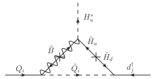
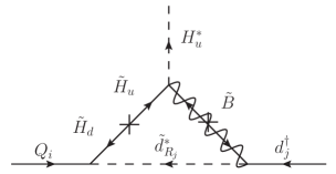
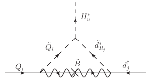
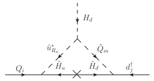
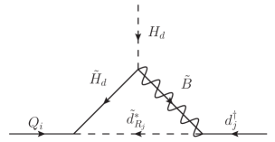
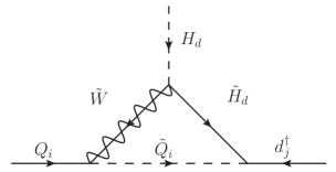
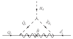
The SUSY threshold corrections can be subdivided into two classes: While at tree-level the down-type quarks only couple to the Higgs field , via exchange of sparticles at one-loop level they can also couple to , as shown in Figure 3 in section 3. When the sparticles are integrated out the emerging effective operator is enhanced for large (i.e. “-enhanced”). Analogously, there are also -enhanced threshold corrections to the charged lepton Yukawa couplings. For , however, the threshold effects emerging from effective couplings to are -suppressed. The second class of threshold corrections emerges from the supersymmetric loops shown in Figure 4. While some of them are strongly suppressed, others lead to the emergence of effective operators proportional to the soft SUSY-breaking trilinear couplings. For large trilinear couplings, they too can become important. Given the importance of the SUSY threshold corrections, we will discuss them and their implementation in SusyTC in detail in the next section.
{floatrow}\capbtabbox
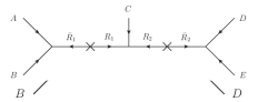
Figure 1: Dimension 5 effective operators and CG factors emerging from the supergraphs of Figure 2 when and are integrated out [5].
\ffigbox
Figure 2: Supergraphs corresponding to the operators of Table 2 generating effectively Yukawa couplings when the pair of messengers fields
and is integrated out.
We follow the notation of REAP[1] (see also [21]) and use a RL convention for the Yukawa matrices. The MSSM superpotential extended by a type-I seesaw mechanism [22] is thus given by
(2)
where the left-chiral superfields contain the charge conjugated fields and . We use the totally antisymmetric tensor for the product . The soft-breaking Lagrangian is given by
(3)
Note that these conventions differ from SUSY Les Houches Accord 2 [23]. They can easily be translated by
REAP & SusyTC
SLHA 2
Since REAP includes the RG running in the type-I seesaw extension of the MSSM (with the two-loop -functions for the MSSM parameters and the neutrino mass operator given in [21]), we have calculated the two-loop -functions of the gaugino mass parameters , the trilinear couplings , the sfermion squared mass matrices , and soft-breaking Higgs mass parameters and in the presence of , and (using the general formulas of [24]). We list these -functions in appendix A.
The Yukawa matrices and soft-breaking parameters are evolved to the SUSY scale
(4)
where the stop masses are defined by the up-type squark mass eigenstates with the largest mixing to and .444SusyTC can also be set to use the convention or a user-defined SUSY scale, as described in appendix C.REAP automatically integrates out the right-handed neutrinos, as described in [1]. We assume that is much larger than the SUSY scale . REAP also features the possibility to add one-loop right-handed neutrino thresholds for the SM parameters, following [25].
At the SUSY scale the tree-level sparticle masses and mixings are calculated. Considering heavy sparticles and large the SUSY threshold corrections are calculated in the electroweak (EW) unbroken phase. In the EW unbroken phase there are in total twelve types of loop diagrams contributing to the SUSY threshold corrections for (cf. Figures 2 and 3). The SUSY threshold corrections to are calculated in the basis of diagonal squark masses and are given by
(5)
where
(6)
correspond to the -enhanced loops of Figure 3, and
(7)
correspond to the loops in Figure 4, respectively, where the contributions and can become important in cases of small and large trilinear couplings. The loop functions and are defined as
(8)
(9)
, are the Yukawa- and trilinear coupling matrices rotated into the basis where the squark mass matrices are diagonal, using the transformations
(10)
and analogously for down-type (s)quarks and charged (s)leptons.
Figure 3: - enhanced SUSY threshold corrections to .
Figure 4: None - enhanced SUSY threshold corrections to .
The SUSY threshold corrections to are given by
(11)
with the -enhanced contributions
(12)
and
(13)
The diagrams for the SUSY threshold corrections are analogous to the ones in Figures 3 and 4, with the exception that the loop diagrams shown in the top rows do not exist.
Turning to , the types of diagrams which were -enhanced for and are now -suppressed. However, there also exist SUSY threshold corrections which are independent of and enhanced by large trilinear couplings. These SUSY threshold corrections to can have important effects. For example the SUSY threshold corrections to the top Yukawa coupling can be of significance in analyses of the Higgs mass and vacuum stability. The expression for the SUSY threshold corrections can be readily obtained from the SUSY threshold corrections to (3)–(3) by the replacement
(14)
with the exception of the bino-loops, whose contribution become
(15)
due to the different hypercharges of the (s)particles in the loop. The loop diagrams are identical to the ones of Figure 3 and 4, with exchanged by .
Finally SusyTC calculates the value of and from , , and by requiring the existence of spontaneously broken EW vacuum, which is equivalent to vanishing one-loop corrected tad-pole equations of and
(16)
with and . In the real (CP conserving) MSSM the phase is restricted to and . The expressions for the one-loop tadpoles , and the transverse Z-boson self energy are based on [26], but extended to include inter-generational mixing, and are presented in appendix B. Because enters the one-loop formulas for the threshold corrections, treating , and as functions of tree-level parameters is sufficiently accurate. The one-loop expression of the soft-breaking mass is calculated as
(17)
If desired, SusyTC allows to outsource a two-loop Higgs mass calculation to external software, e.g. FeynHiggs[27, 28, 29], by calculating the pole mass () as input for the complex (real) MSSM
(18)
(19)
where is the W-boson mass given as
(20)
with and pole masses and the vacuum expectation value given by
(21)
As in the previous formulas, the self energies and are based on [26], but extended to include inter-generational mixing, and are understood as functions of tree-level parameters. They are given in appendix B.
4 The REAP extension SusyTC
In this section we provide a “Getting Started” calculation for SusyTC. A full documentation of all features is included in appendix C. Since SusyTC is an extension to REAP, an up-to-date version of REAP-MPT[1] (available at http://reapmpt.hepforge.org) needs to be installed on your system. SusyTC consists out of the REAP model file RGEMSSMsoftbroken.m, which is based on the model file RGEMSSM.m of REAP 1.11.2 and additionally contains, among other things, the RGEs of the MSSM soft-breaking parameters and the matching to the SM, and the file SusyTC.m, which includes the formulas for the sparticle spectrum and SUSY threshold correction calculations. Both files can be downloaded from http://particlesandcosmology.unibas.ch/pages/SusyTC.htm and have to be copied into the REAP directory.
To begin a calculation with SusyTC, one first needs to import RGEMSSMsoftbroken.m:
Needs["REAP‘RGEMSSMsoftbroken‘"];
The model MSSMsoftbroken is then defined by RGEAdd, including additional options such as RGEtan:
RGEAdd["MSSMsoftbroken",RGEtan 30];
In MSSMsoftbroken all REAP options of the model MSSM are available. The options additionally available in SusyTC are given in appendix C. The input is given by RGESetInitial. Let us illustrate some features of SusyTC: To test for example the GUT scale prediction for the Yukawa coupling ratio , considering a given example parameter point in the Constrained MSSM, one can type:
Of course, any general matrices can be used as input for the Yukawa, trilinear, and soft-breaking matrices, as given by the specific SUSY flavour GUT model under consideration. Also, non-universal gaugino masses can be specified.
The RGEs are then solved from the GUT scale to the Z-boson mass scale by
RGESsolve[91,210∧16];
The ratio of the and strange quark Yukawa couplings at the Z-boson mass scale can now be obtained with RGEGetSolution, CKMParameters, and MNSParameters:
Yu = RGEGetSolution[91, RGEYu];
Yd = RGEGetSolution[91, RGEYd];
Ye = RGEGetSolution[91, RGEYe];
M = RGEGetSolution[91, RGEM];
MNSParameters[M,Ye][[3, 2]]/CKMParameters[Yu, Yd][[3, 2]]
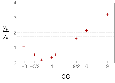
Repeating this calculation with all CG factors listed in Table 2 of [5], one obtains the results shown in Figure 5.
Figure 5: Example results for at the electroweak scale, considering the GUT-scale CG factors from Table 2 of [5], i.e. the GUT predictions , for a given example Constrained MSSM parameter point with , , , and . The area between the dashed gray lines corresponds to the experimental range [11].
As described in appendix C, SusyTC can also read and write “Les Houches” files [23, 30] as input and output.
5 The Sparticle Spectrum predicted from CG factors
In this section we apply SusyTC to investigate the constraints on the sparticle spectrum which arise from a set of GUT scale predictions for the quark-lepton Yukawa coupling ratios , , and . As GUT scale boundary conditions for the SUSY-breaking terms we take the Constrained MSSM. The experimental constraints are given by the Higgs boson mass [31] as well as the charged fermion masses (and the quark mixing matrix).
We use the experimental constraints for the running Yukawa couplings at the Z-boson mass scale calculated in [11], where we set the uncertainty of the charged lepton Yukawa couplings to one percent to account for the estimated theoretical uncertainty (which here exceeds the experimental uncertainty). When applying the measured Higgs mass as constraint, we use a 1 interval of , including the estimated theoretical uncertainty.
For our study, we consider GUT scale Yukawa coupling matrices which feature the GUT-scale Yukawa relations , , and (cf. [5]):
(22)
These GUT relations can emerge as direct result of CG factors in SU(5) GUTs or as approximate relation after diagonalization of the GUT-scale Yukawa matrices and (cf. [9, 10, 17, 18]). For the soft-breaking parameters we restrict our analysis to the Constrained MSSM parameters , , and , with determined from requiring the breaking of electroweak symmetry as in (16) and set . We note that in specific models for the GUT Higgs potential, for instance in [17], can be realized as an effective parameter of the superpotential with a fixed phase, including the case that is real. The value of is fixed at the SUSY scale to .555We have not included in the fit, however we tried different values and turned out to be the best choice for obtaining a good fit.
We note that we have also added a neutrino sector, i.e. a neutrino Yukawa matrix and and a mass matrix of the right-handed neutrinos, but we have set the entries of to very small values below , such that their effects on the RG evolution can be safely neglected, and the masses of the right-handed neutrinos to values many orders of magnitude higher than the expected SUSY scale. With these parameters, the neutrino sector is decoupled from the main analysis. Such small values of the neutrino Yukawa couplings are e.g. expected in the models [9, 10, 18], where they arise as effective operators.
Using one-loop RGEs, REAP 1.11.2 and SusyTC we determine the soft-breaking parameters and at the SUSY scale, as well as the pole mass . This output is then passed to FeynHiggs 2.11.2 [27, 28, 29] in order to calculate the two-loop corrected pole masses of the Higgs bosons in the complex MSSM. The MSSM is automatically matched to the SM and we compare the results for the Yukawa couplings at the Z-boson mass scale with the experimental values reported in [11].
When fitting the GUT-scale parameters to the experimental data, we found that our results for the up-type quark Yukawa couplings and CKM angles and CP-phase could be fitted to agree with observations to at least relative precision, by adjusting the parameters of . The remaining six parameters are used to fit the Yukawa couplings of down-type quarks and charged leptons, as well as the mass of the SM-like Higgs boson. We find a benchmark point with a :
input GUT-scale parameters
low energy results
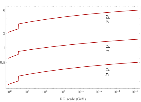
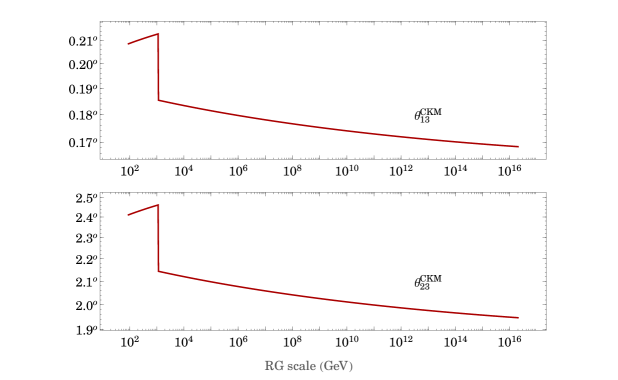
Looking at our results for the low-energy Yukawa coupling ratios, , , and , the importance of SUSY threshold corrections in evaluating the GUT-scale Yukawa ratios becomes evident. This can also be seen in Figure 6. Additionally, as shown in Figure 7, SUSY threshold corrections also affect the CKM mixing angles. Finally, in Figure 8 we show the results for the RG running of the soft-breaking mass parameters.
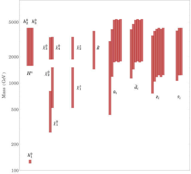
The SUSY spectrum obtained by SusyTC is shown in Figure 9.
The lightest supersymmetric particle (LSP) is a bino-like neutralino of about 445 . The next-to-lightest supersymmetric particle (NLSP) is a stop of about 656 . The SUSY scale is obtained as . The parameter obtained from requiring spontaneous electroweak symmetry breaking is given by . Note that the only experimental constraints we used were the results for quark and charged lepton masses as well as . In particular, no bounds on the sparticle masses were applied as well as no restrictions from the neutralino relic density (which would require further assumptions on the cosmological evolution).
Due to the large (absolute) values of the trilinear couplings, we find using the constraints from [32], that the vacuum of our benchmark point is meta-stable. The scalar potential possesses charge and colour breaking (CCB) vacua, as well as one “unbounded from below” (UFB) field direction in parameter space. However, estimating the stability of the vacuum via the Euclidean action of the “bounce” solution [33, 34] (following [35]) shows that the lifetime of the vacuum is many orders larger than the age of the universe.
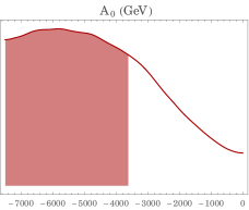
Confidence intervals for the sparticle masses are obtained as Bayesian “highest posterior density” (HPD) intervals666An HPD interval is the interval [,] such that and the posterior probability density inside the interval is higher than for any outside of the interval [31]. from a Markov Chain Monte Carlo sample of two million points, using a Metropolis algorithm. As additional constraint we restricted to avoid possibly dangerous vacuum decay rates. The HPD intervals for the Constrained MSSM soft-breaking parameters are shown in Figure 10. The HPD results of the sparticle masses are shown in Figure 11. As for the benchmark point, for all other parameter points the LSP and NLSP are a neutralino and stop, respectively. The HPD interval for the SUSY scale is obtained as .
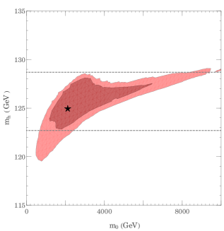
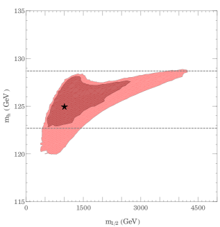
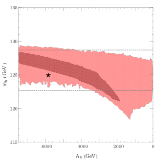
In Figure 12, we show two-dimensional HPD regions for the correlations between Constrained MSSM soft-breaking parameters and the mass of the Higgs bosons.
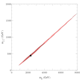
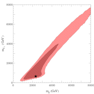
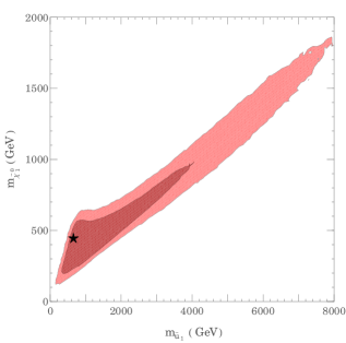
Finally, in Figure 13 we show the two-dimensional HPD regions for the correlations between the masses of the lightest stop, the neutralino LSP, and the gluino.
6 Summary and Conclusion
In this work we discussed how predictions for the sparticle spectrum can arise from GUTs, which feature predictions for the ratios of quark and lepton Yukawa couplings at high energy. To test them by comparing with the experimental data, the RG running between high and low energy has to be performed with sufficient accuracy, including threshold corrections. In SUSY theories, the one-loop threshold corrections when matching the SUSY model to the SM are of particular importance, since they can be enhanced by or large trilinear couplings, and thus have the potential to strongly affect the quark-lepton mass relations. Since the SUSY threshold corrections depend on the SUSY parameters, they link a given GUT flavour model to the SUSY model. In other words, via the SUSY threshold corrections, GUT models can predict properties of the sparticle spectrum from the pattern of quark-lepton mass ratios at the GUT scale.
To accurately study such predictions, we extend and generalize various formulas in the literature which are needed for a precision analysis of SUSY flavour GUT models: For example, we extend the RGEs for the MSSM soft breaking parameters at two-loop by the additional terms in the seesaw type-I extension (cf. appendix A). We generalize the one-loop calculation of and pole mass calculation of and to include inter-generational mixing in the self energies (cf. appendix B). Furthermore, we calculate the full one-loop SUSY threshold corrections for the down-type quark, up-type quark and charged lepton Yukawa coupling matrices in the electroweak unbroken phase (cf. section 3).
We introduce the new software tool SusyTC, a major extension to the Mathematica package REAP, where these formulas are implemented. In addition, SusyTC calculates the sparticle spectrum and the SUSY scale , and can provide output in SLHA “Les Houches” files which are the necessary input for external software, e.g. for performing a two-loop Higgs mass calculation. REAP extended by SusyTC accepts general GUT scale Yukawa, trilinear and soft breaking mass matrices as well as non-universal gaugino masses as input, performs the RG evolution (integrating out the right-handed neutrinos at their mass thresholds in the type I seesaw extension of the MSSM) and automatically matches the MSSM to the SM, making it a convenient tool for top-down analyses of SUSY flavour GUT models.
We applied SusyTC to study the predictions for the parameters of the Constrained MSSM SUSY scenario from the set of GUT-scale Yukawa relations , , and , which has been proposed recently in the context of GUT flavour models. With a Markov Chain Monte Carlo analysis we find a “best-fit” benchmark point where the LSP is a bino-like neutralino with a mass of about and the NLSP a stop with a mass of . We also find the 1 Bayesian confidence intervals for the sparticle masses and the correlations between the SUSY parameters. Without applying any constraints from LHC SUSY searches or dark matter, we find that the considered GUT scenario predicts a sparticle spectrum above past LHC sensitivities, but within reach of the current LHC run or a future high-luminosity upgrade.
Acknowledgements
We would like to thank Vinzenz Maurer for help with code optimisation and Christian Hohl for testing. We also thank Eros Cazzato, Thomas Hahn, Vinzenz Maurer, Stefano Orani and Sebastian Paßehr for useful discussions. This work has been supported by the Swiss National Science Foundation.
Figure 6: RG evolution of the Yukawa coupling ratios of the first, second, and third family from the GUT-scale to the mass scale of the Z-boson. The GUT scale parameters correspond to our benchmark point from Section 5. The effects of the threshold corrections are clearly visible at the SUSY scale .Figure 7: RG evolution of the CKM mixing angles and from the GUT-scale to the mass scale of the Z-boson. The GUT scale parameters correspond to our benchmark point from Section 5. The effects of the threshold corrections are clearly visible at the SUSY scale .Figure 8: RG evolution of the soft-breaking gaugino masses (solid black), squark masses (red), slepton masses (yellow), and and (dashed black), from the GUT-scale to the SUSY scale . The GUT scale parameters correspond to our benchmark point from Section 5. Figure 9: SUSY spectrum with GUT scale boundary conditions , , and , corresponding to our benchmark point from Section 5.
Figure 10: HPD intervals for the Constrained MSSM soft-breaking parameters.Figure 11: HPD intervals for the sparticle spectrum and Higgs boson masses with GUT scale boundary conditions , , and , corresponding to our benchmark point from Section 5. The LSP is always and the NLSP is always a stop.
Figure 12: 2D (dark) and (bright) HPD regions for Constrained MSSM soft-breaking parameters and the Higgs mass. The black star marks the benchmark point. The dashed lines correspond to the region .
Figure 13: 2D (dark) and (bright) HPD regions for the masses ofthe neutralino, gluino, and stop. The black star marks the benchmark point.
Appendix A The -functions in the seesaw type-I extension of the MSSM
In this appendix we list the -functions of the SUSY soft-breaking parameters in the MSSM extended by the additional terms in the seesaw type-I extension (obtained using the general formulas of [24]). Our conventions for and are given in (3) and (3).
A.1 One-Loop -functions
(23)
(24)
(25)
(26)
(27)
(28)
(29)
(30)
(31)
(32)
(33)
(34)
(35)
(36)
(37)
with
(38)
A.2 Two-Loop -functions
(39)
(40)
(41)
(42)
(43)
(44)
(45)
(46)
(47)
(48)
(49)
(50)
(51)
(52)
(53)
with
(54)
(55)
(56)
and
(57)
Appendix B Self-energies and one-loop tadpoles including inter-generational mixing
Here we present the used formulas for the self-energies , , , and the one-loop tadpoles , , which are based on [26] but generalized to include inter-generational mixing. In this appendix we employ SLHA 2 conventions [23] in the Super-CKM and Super-PMNS basis, to agree with the convention of [26]. The soft-breaking mass matrices in the Super-CKM/Super-PMNS basis are obtained from our flavour basis conventions (3) and (3) by
(58)
Let us briefly review our generalization to the sfermion mass matrices of [26]: We define the sfermion mixing matrices by777The SLHA 2 convention sfermion mixing matrices can be obtained via .
(59)
with the sfermion mass matrices in the Super-CKM/Super-PMNS basis
(60)
The D-terms are given by
(61)
where denotes the isospin and the electric charge of the flavour , and denotes the weak mixing angle. Note that our convention for differs by a sign from the convention in [26].
For the sake of completeness we also list the conventions for neutralino and chargino mass matrices and mixing matrices: The neutralino mixing matrix is defined by
(62)
with
(63)
The chargino mixing matrix is defined by
(64)
with
(65)
We now present the generalization of , , , , and of [26] to include inter-generational mixing. For all we have checked that our equations reduce to the corresponding equations in [26] when
The conventions for the one-loop scalar functions , , , , , and [36] are adopted from appendix B of [26]. Summations are over all fermions, whereas summations , are restricted to up-type and down-type fermions, respectively. Summations , are over (s)quark doublets, and analogously for (s)leptons. In summations over sfermions the indices , , , and run from 1 to 6 for , , and and from 1 to 3 for . In summations of neutralinos (charginos) the indices , run from 1 to 4 (2). The summations runs over all neutral Higgs- and Goldstone bosons, the summation over the charged ones.
(73)
The couplings , , , and are given in Eqs. (A.7) and (D.5) of [26].
(74)
The couplings and are given in Eq. (D.70) and Eqs. (D.39-D.42) of [26]. The couplings , , and are defined in Eqs. (D.63-D.65) and Eq. (D.67) of [26]. The couplings to sfermions in the case of inter-generational mixing are given by
(75)
(76)
(77)
(78)
(79)
The couplings , , , and are given in Eq. (D.70) and Eqs. (D.34-D.38) of [26]. The couplings , , and are defined in Eqs. (D.63-D.65) and Eq. (D.67) of [26]. The couplings to sfermions in the case of inter-generational mixing are given by
(80)
(81)
(82)
(83)
(84)
(85)
The couplings to sfermion in the case of inter-generational mixing are given by
(86)
(87)
(88)
(89)
The couplings to sfermion in the case of inter-generational mixing are given by
(90)
(91)
Appendix C SusyTC documentation
Here we present a documentation of the REAP extension SusyTC. To get started, please follow first the steps described in Section 4.
We now describe that additional features of SusyTC:
In addition to the features of REAP package RGEMSSMsoftbroken.m (described in the REAP documentation), SusyTC adds the following options to the command RGEAdd:
•
STCsign is the general factor in front of in (16). (default: )
•
STCcMSSM is a switch to change between the CP-violating (complex) MSSM and CP-conserving (real) MSSM. (default: True)
•
STCSusyScale sets the SUSY scale (in ), where the MSSM is matched to the SM. If set to "Automatic", SusyTC determines automatically from the sparticle spectrum. (default: "Automatic")
•
STCSusyScaleFromStops is a switch to choose whether SusyTC calculates the SUSY scale as geometric mean of the stop masses ,
where the stop masses are defined by the up-type squark mass eigenstates with the largest mixing to and , or as geometric mean of the lightest and heaviest up-type squarks . Without effect if STCSusyScale is not set to "Automatic". (default: True)
•
STCSearchSMTransition is a switch to enable or disable the matching to the SM and the calculation of supersymmetric threshold corrections and sparticle spectrum. (default: True)
•
STCCCBConstraints is a switch to enable or disable a warning message for potentially dangerous charge and colour breaking vacua, if large trilinear couplings violate the constraints of [37] at the SUSY scale
(92)
where , and denote the soft-breaking mass parameters of the scalar fields associated with the trilinear coupling in the basis of diagonal Yukawa matrices. (default: True)
•
STCUFBConstraints is a switch to enable or disable a warning message for possibly dangerous “unbounded from below” directions in the scalar potential, if the constraints of [32] are violated at the SUSY scale
(93)
(94)
evaluated in the basis of (3). Note that the UFB-I constraint is automatically satisfied, since SusyTC calculates from , , , and by requiring the existence of electroweak symmetry breaking. (default: True)
In addition to the parameters known from the MSSMREAP model, the following soft-breaking parameters are available as input for RGESetInitial:
•
RGETu, RGETd, RGETe, and RGET are the soft-breaking trilinear coupling matrices. If given, the Constrained MSSM parameter RGEA0 for the corresponding trilinear coupling is overwritten. (default: Constrained MSSM)
•
RGEM1, RGEM2, and RGEM3 are the soft-breaking gaugino mass parameters. If given, the Constrained MSSM parameter RGEM12 for the corresponding gaugino is overwritten. (default: Constrained MSSM)
•
RGEm2Q, RGEm2L, RGEm2u, RGEm2d, RGEm2e, RGEm2 are the soft-breaking squared mass matrices for the sfermions. If given, the Constrained MSSM parameter RGEm0 for the corresponding scalar masses is overwritten. (default: Constrained MSSM)
•
RGEm2Hd and RGEm2Hu are the soft-breaking squared masses for and , respectively. If given, the Constrained MSSM parameter RGEm0 for the corresponding scalar mass is overwritten. (default: Constrained MSSM)
•
RGEM12 is the Constrained MSSM parameter for gaugino mass parameters in GeV. (default: 750)
•
RGEm0 is the Constrained MSSM parameter for all soft-breaking masses of scalars in GeV. (default: 1500)
•
RGEA0 is the Constrained MSSM parameter for trilinear couplings, e.g. . (default: -500)
An example for an input at the GUT scale would be
RGESetInitial[210^16,RGEM1->863,RGEM2->131,
RGEM3->-392,RGESuggestion->"GUT"];
The solution at a lower energy scale such as can now be obtained by the REAP command RGESolve:
RGESolve[91.19,210^16];
Some parameter points might lead to tachyonic sparticle masses. In such instances the evaluation of SusyTC is stopped and an error message is returned using the Mathematica command Throw. In order to properly catch such error messages, we therefore recommend to use instead
Catch[RGESolve[91.19,210^16],TachyonicMass];
In addition to the parameters known from the MSSMREAP model, the following soft-breaking parameters are available for RGEGetSolution at all energy scales higher than the SUSY scale :
•
RGETu, RGETd, RGETe, and RGET are used to get the soft-breaking trilinear coupling matrices.
•
RawT is used to get the raw (internal representation) of the soft-breaking trilinear matrix for sneutrinos.
•
RGEM1, RGEM2, and RGEM3 are used to get the soft-breaking gaugino mass parameters.
•
RGEm2Q, RGEm2L, RGEm2u, RGEm2d, RGEm2e, RGEm2 are used to get the soft-breaking squared mass matrices for the sfermions.
•
RGEm2Hd and RGEm2Hu are used to get the soft-breaking squared masses for and , respectively.
To obtain the running gluino mass at a scale of two TeV for example, one uses
RGEGetSolution[2000,RGEM3];
With SusyTC the sparticle spectrum is automatically calculated. The following functions are included in SusyTC:
•
STCGetSUSYScale[] returns the SUSY scale .
•
STCGetSUSYSpectrum[] returns a list of replacement rules for the SUSY scale , the tree-level values of and , and the sparticle masses and (tree-level) mixing matrices at the SUSY scale. In detail it contains
–
"Q" the SUSY scale .
–
"","" the values of and .
–
"M1","M2","M3" are the gaugino mass parameters.
–
"Mh","MH","MA","MHp" the (tree-level) masses of the MSSM Higgs bosons.888Note that there is no CP-violation in the MSSM Higgs sector on tree-level.
–
"m0" a list of the four neutralino masses.
–
"mp" a list of the two chargino masses.
–
"msude" a 36 array of the six up-type quarks, down-type squarks and charged slepton masses, respectively.
–
"ms" a list of the three light sneutrino masses.
–
"W" the weak mixing angle.
–
"tan" the mixing angle of the CP-even Higgs bosons.
–
"N" the mixing matrix of neutralinos.
–
"U","V" the mixing matrices for charginos.
–
"Wude" a list of the three sparticle mixing matrices for up-type squarks, down-type squarks and charged sleptons.
–
"W" the mixing matrix of the three light sneutrinos.
To obtain for example the SUSY scale and the tree-level masses of the charginos call
"Q"/.STCGetSUSYSpectrum[];
"mp"/.STCGetSUSYSpectrum[];
The squark masses and charged slepton masses are contained in a joint list as {,,}, and analogously for the sfermion mixing matrices. To obtain for example the up-type squark masses, the charged slepton mixing matrix, and the sneutrino masses type
("msude"/.STCGetSUSYSpectrum[])[[1]];
("Wude"/.STCGetSUSYSpectrum[])[[3]];
"ms"/.STCGetSUSYSpectrum[];
•
STCGetOneLoopValues[] returns a list of replacement rules containing
–
"","" the one-loop corrected -parameter and as in (16) and (17) at the SUSY scale .
–
"vev" the one-loop vev as in (21) at the SUSY scale .
–
"MHp" ("MA") the pole-mass () of the charged (CP-odd) Higgs boson for STCcMSSM = True (False).
The value of can for example be obtained from
""/.STCGetOneLoopValues[];
•
STCGetSCKMValues[] returns a list of replacement rules with the soft-breaking mass squared and trilinear coupling matrices in the SCKM basis, where sparticles are rotated analogously with their corresponding superpartners999We use the term “SCKM” for the super CKM and super PMNS basis.. Since they are used for the self-energies calculation as described in the previous appendix, they are returned in SLHA2 convention [23]! In detail, there are
–
"VCKM" the CKM mixing matrix.
–
"VPMNS" the PMNS mixing matrix.
–
SCKMBasis["m2Q"], SCKMBasis["m2u"], SCKMBasis["m2d"] the squark soft-breaking mass squared matrices in the super CKM basis with SLHA2 convetions.
–
SCKMBasis["m2L"], SCKMBasis["m2e"] the slepton soft-breaking mass squared matrices in the super PMNS basis with SLHA2 conventions.
–
SCKMBasis["T"] a list of the three trilinear coupling matrices for up-type squarks, down-type squarks and charged sleptons in the SCKM basis with SLHA2 conventions.
–
SCKMBasis["Y"] a 33 array of the Yukawa coupling singular values for up-type squarks, down-type squarks and charged sleptons.
To obtain the down-type trilinear coupling matrix and the mass squared matrix of the left-handed up-type squarks in the SLHA basis for example, type
(SCKMBasis["T"]/.STCGetSCKMValues[])[[2]];
SCKMBasis["mQ2u"]/.STCGetSCKMValues[];
•
STCGetInternalValues[] returns everything that is internally used for the calculation of the threshold corrections and sparticle spectrum, i.e. the results from STCGetSCKMValues[] and STCGetSUSYSpectrum[] with the one-loop corrected parameters from STCGetOneLoopValues[] replacing tree-level ones if available. We recommend to the user to use those separate functions instead.
As additional feature, SusyTC optionally supports input and output as SLHA “Les Houches” files. These files follow SLHA conventions [30, 23]:
•
STCSLHA2Input[“Path”] loads an “Les Houches” input file stored in “Path” and executes REAP and SusyTC. If no path is given, the default path is assumed as “SusyTC.in” in the Mathematica Notebook Directory. An important difference to other spectrum calculators is the pure “top-down” approach by SusyTC, i.e. there is no attempt of fitting SM inputs at a low scale or calculating a GUT-scale from gauge couplings unification. Instead, all input is given at a user-defined high energy scale, which is then evolved to lower scales. The input should be given in the flavour basis in SLHA 2 convention [23], with analogous convention for and convention for as in (3). The relation between the SusyTC conventions and the SLHA 2 conventions is given in Section 3. In the following, we list all SLHA 2 input blocks, which are available in SusyTC:
–
Block MODSEL: The only available switch is: 5 : (Default = 2) CP violation (STCcMSSM)
–
Block SusyTCInput: Switches (1=True, 0=False) are defined for RGEAdd[]: 1 : (Default = 1) STCSusyScaleFromStops
2 : (Default = 1) STCSearchSMTransition
3 : (Default = 1) STCCCBConstraints
4 : (Default = 1) STCUFBConstraints
5 : (Default = 1) Print a Warning in case of Tachyonic masses 6 : (Default = 1) One or Two Loop RGEs
–
Block MINPAR: Constrained MSSM parameters as defined in [30, 23]. Note however, that the input value of is interpreted to be given at the SUSY scale.
–
Block IMMINPAR: Reads the in case of the complex MSSM: 4 :
–
Block EXTPAR: 0 : (Default = ): Input scale Note that with SusyTC an automatic calculation of the GUT scale is not possible. The remainder of the block works as usual, e.g. optionally one can overwrite common Constrained MSSM gaugino or Higgs soft-breaking parameters: 1 : bino mass (real part) 2 : wino mass (real part) 3 : gluino mass (real part) 21 : 22 : Imaginary components for the gaugino masses can be given in Block IMEXTPAR.
Block QEXTPAR: low energy input: 0 : (Default = ): The low energy scale to which REAP evolves the SM RGEs. 23 : “SUSY scale” , where the MSSM is matched to the SM. If this entry is set, it overwrites the automatically calculated SUSY scale.
–
Block GAUGE: the gauge couplings at the input scale 1 : gauge coupling 2 : gauge coupling 3 : gauge coupling
–
Block YU, Block YD, Block YE, Block YN: The real parts of the Yukawa matrices , , , and in the flavour basis [23]. They should be given in the FORTRAN format (1x,I2,1x,I2,3x,1P,E16.8,0P,3x,‘#’,1x,A), where the first two integers correspond to the indices and the double precision number to .
–
Block IMYU, Block IMYD, Block IMYE, Block IMYN: The imaginary parts of the Yukawa matrices , , , and in the flavour basis [23]. They are given in the same format as the real parts.
–
Block MN: The real part of the symmetric Majorana mass matrix of the right-handed neutrinos in the flavour basis (3). Only the “upper-triangle” entries should be given, the input format is as for the Yukawa matrices.
–
Block IMMN: The imaginary part of the symmetric Majorana mass matrix of the right-handed neutrinos in the flavour basis (3). Only the “upper-triangle” entries should be given, the input format is as for the Yukawa matrices.
The remaining blocks can be given optionally to overwrite Constrained MSSM input boundary conditions:
–
Block TU, Block TD, Block TE, Block TN: The real parts of the trilinear soft-breaking matrices , , , and in the flavour basis [23]. They should be given in the same format as the Yukawa matrices.
–
Block IMTU, Block IMTD, Block IMTE, Block IMTN: The imaginary parts of the trilinear soft-breaking matrices , , , and in the flavour basis [23]. They should be given in the same format as the Yukawa matrices.
–
Block MSQ2, Block MSU2, Block MSD2, Block MSL2, Block MSE2,
Block MSN2: The real parts of the soft-breaking mass squared matrices , , , , , and in the flavour basis [23]. Only the “upper-triangle” entries should be given, the input format is as for the Yukawa matrices.
–
Block IMMSQ2, Block IMMSU2, Block IMMSD2,Block IMMSL2,
Block IMMSE2, Block IMMSN2: The imaginary parts of the soft-breaking mass squared matrices , , , , , and in the flavour basis [23]. Only the “upper-triangle” entries should be given, the input format is as for the Yukawa matrices.
•
STCWriteSLHA2Output[“Path”] writes an “Les Houches” [30, 23] output file to “Path”. If no path is given, the output is saved in the Mathematica Notebook directory as “SusyTC.out”. The output follows SLHA conventions, with the following exceptions:
–
Block MASS: The mass spectrum is given as masses at the SUSY scale. The only exception is the pole mass () for CP violation turned on (off).
–
Block ALPHA: the tree-level Higgs mixing angle .
–
Block HMIX: Instead of we give 101 :
The other blocks follow the SLHA2 output conventions, e.g. values at the SUSY scale in the Super-CKM/Super-PMNS basis. To avoid confusion, the blocks Block DSQMIX, Block USQMIX, Block SELMIX, Block SNUMIX and the corresponding blocks for the imaginary entries, return the sfermion mixing matrices in SLHA 2 convention.
References
[1]
S. Antusch, J. Kersten, M. Lindner, M. Ratz and M. A. Schmidt,
JHEP 0503 (2005) 024
[hep-ph/0501272].
[2]
R. Hempfling,
Phys. Rev. D 49 (1994) 6168,
L. J. Hall, R. Rattazzi and U. Sarid,
Phys. Rev. D 50 (1994) 7048
[hep-ph/9306309],
M. Carena, M. Olechowski, S. Pokorski and C. E. M. Wagner,
Nucl. Phys. B 426 (1994) 269
[hep-ph/9402253];
T. Blazek, S. Raby and S. Pokorski,
Phys. Rev. D 52 (1995) 4151
[hep-ph/9504364],
S. Antusch and M. Spinrath,
Phys. Rev. D 78 (2008) 075020
[arXiv:0804.0717 [hep-ph]].
[3]
L. E. Ibanez and G. G. Ross,
Phys. Lett. B 105 (1981) 439,
M. B. Einhorn and D. R. T. Jones,
Nucl. Phys. B 196 (1982) 475,
J. R. Ellis, D. V. Nanopoulos and S. Rudaz,
Nucl. Phys. B 202 (1982) 43,
S. Dimopoulos and H. Georgi,
Nucl. Phys. B 193 (1981) 150.
[4]
H. Georgi and C. Jarlskog,
Phys. Lett. B 86 (1979) 297.
[5]
S. Antusch and M. Spinrath,
Phys. Rev. D 79 (2009) 095004
[arXiv:0902.4644 [hep-ph]].
[6]
S. Antusch, S. F. King and M. Spinrath,
Phys. Rev. D 89 (2014) 5, 055027
[arXiv:1311.0877 [hep-ph]].
[7]
G. Ross and M. Serna,
Phys. Lett. B 664 (2008) 97
[arXiv:0704.1248 [hep-ph]],
W. Altmannshofer, D. Guadagnoli, S. Raby and D. M. Straub,
Phys. Lett. B 668 (2008) 385
[arXiv:0801.4363 [hep-ph]],
I. Gogoladze, R. Khalid, S. Raza and Q. Shafi,
JHEP 1012 (2010) 055
[arXiv:1008.2765 [hep-ph]],
S. Antusch, L. Calibbi, V. Maurer and M. Spinrath,
Nucl. Phys. B 852 (2011) 108
[arXiv:1104.3040 [hep-ph]],
H. Baer, I. Gogoladze, A. Mustafayev, S. Raza and Q. Shafi,
JHEP 1203 (2012) 047
[arXiv:1201.4412 [hep-ph]],
H. Baer, S. Raza and Q. Shafi,
Phys. Lett. B 712 (2012) 250
[arXiv:1201.5668 [hep-ph]],
A. Anandakrishnan, S. Raby and A. Wingerter,
Phys. Rev. D 87 (2013) 5, 055005
[arXiv:1212.0542 [hep-ph]],
M. Adeel Ajaib, I. Gogoladze, Q. Shafi and C. S. Un,
JHEP 1307 (2013) 139
[arXiv:1303.6964 [hep-ph]],
N. Okada, S. Raza and Q. Shafi,
Phys. Rev. D 90 (2014) 1, 015020
[arXiv:1307.0461 [hep-ph]],
A. Anandakrishnan, B. C. Bryant, S. Raby and A. Wingerter,
Phys. Rev. D 88 (2013) 075002
[arXiv:1307.7723],
B. Bajc, S. Lavignac and T. Mede,
AIP Conf. Proc. 1604 (2014) 297
[arXiv:1310.3093 [hep-ph]],
M. A. Ajaib, I. Gogoladze, Q. Shafi and C. S. Ün,
JHEP 1405 (2014) 079
[arXiv:1402.4918 [hep-ph]],
A. Anandakrishnan, B. C. Bryant and S. Raby,
Phys. Rev. D 90 (2014) 1, 015030
[arXiv:1404.5628 [hep-ph]],
A. Anandakrishnan, B. C. Bryant and S. Raby,
JHEP 1505 (2015) 088
[arXiv:1411.7035 [hep-ph]],
I. Gogoladze, A. Mustafayev, Q. Shafi and C. S. Un,
Phys. Rev. D 91 (2015) 9, 096005
[arXiv:1501.07290 [hep-ph]],
Z. Poh and S. Raby,
Phys. Rev. D 92 (2015) 1, 015017
[arXiv:1505.00264 [hep-ph]],
Z. Berezhiani, M. Chianese, G. Miele and S. Morisi,
JHEP 1508 (2015) 083
[arXiv:1505.04950 [hep-ph]],
B. Bajc, S. Lavignac and T. Mede,
arXiv:1509.06680 [hep-ph].
[8]
G. Aad et al. [ATLAS Collaboration],
Phys. Lett. B 716 (2012) 1
[arXiv:1207.7214 [hep-ex]],
S. Chatrchyan et al. [CMS Collaboration],
Phys. Lett. B 716 (2012) 30
[arXiv:1207.7235 [hep-ex]].
[9]
S. Antusch, C. Gross, V. Maurer and C. Sluka,
Nucl. Phys. B 877, 772 (2013)
[arXiv:1305.6612 [hep-ph]].
[10]
S. Antusch, C. Gross, V. Maurer and C. Sluka,
Nucl. Phys. B 879, 19 (2014)
[arXiv:1306.3984 [hep-ph]].
[11]
S. Antusch and V. Maurer,
JHEP 1311 (2013) 115
[arXiv:1306.6879 [hep-ph]].
[12]
H. Baer, F. E. Paige, S. D. Protopopescu and X. Tata,
hep-ph/9305342.
[13]
B. C. Allanach,
Comput. Phys. Commun. 143 (2002) 305
[hep-ph/0104145].
[14]
A. Djouadi, J. L. Kneur and G. Moultaka,
Comput. Phys. Commun. 176 (2007) 426
[hep-ph/0211331].
[15]
W. Porod,
Comput. Phys. Commun. 153 (2003) 275
[hep-ph/0301101],
W. Porod and F. Staub,
Comput. Phys. Commun. 183 (2012) 2458
[arXiv:1104.1573 [hep-ph]].
[16]
A. Djouadi,
hep-ph/0211357.
[17]
S. Antusch, I. de Medeiros Varzielas, V. Maurer, C. Sluka and M. Spinrath,
JHEP 1409 (2014) 141
[arXiv:1405.6962 [hep-ph]].
[18]
J. Gehrlein, J. P. Oppermann, D. Schäfer and M. Spinrath,
Nucl. Phys. B 890 (2014) 539
[arXiv:1410.2057 [hep-ph]].
[19]
A. Meroni, S. T. Petcov and M. Spinrath,
Phys. Rev. D 86 (2012) 113003
[arXiv:1205.5241 [hep-ph]].
[20]
S. Antusch, C. Gross, V. Maurer and C. Sluka,
Nucl. Phys. B 866 (2013) 255
[arXiv:1205.1051 [hep-ph]].
[21]
S. Antusch and M. Ratz,
JHEP 0207 (2002) 059
[hep-ph/0203027].
[22]
P. Minkowski,
Phys. Lett. B 67 (1977) 421;
M. Gell-Mann, P. Ramond and R. Slansky in Sanibel Talk,
CALT-68-709, Feb 1979, and in Supergravity (North Holland,
Amsterdam 1979);
T. Yanagida in Proc. of the Workshop on Unified Theory and
Baryon Number of the Universe, KEK, Japan, 1979;
S.L.Glashow, Cargese Lectures (1979);
R. N. Mohapatra and G. Senjanovic,
Phys. Rev. Lett. 44 (1980) 912;
J. Schechter and J. W. Valle,
Phys. Rev. D 25 (1982) 774.
[23]
B. C. Allanach et al.,
Comput. Phys. Commun. 180 (2009) 8
[arXiv:0801.0045 [hep-ph]].
[24]
S. P. Martin and M. T. Vaughn,
Phys. Rev. D 50 (1994) 2282
[Phys. Rev. D 78 (2008) 039903]
[hep-ph/9311340].
[25]
S. Antusch and E. Cazzato,
JHEP 1512 (2015) 066
[arXiv:1509.05604 [hep-ph]].
[26]
D. M. Pierce, J. A. Bagger, K. T. Matchev and R. j. Zhang,
Nucl. Phys. B 491 (1997) 3
[hep-ph/9606211].
[27]
S. Heinemeyer, W. Hollik and G. Weiglein,
Comput. Phys. Commun. 124 (2000) 76
[hep-ph/9812320];
S. Heinemeyer, W. Hollik and G. Weiglein,
Eur. Phys. J. C 9 (1999) 343
[hep-ph/9812472];
G. Degrassi, S. Heinemeyer, W. Hollik, P. Slavich and G. Weiglein,
Eur. Phys. J. C 28 (2003) 133
[hep-ph/0212020];
M. Frank, T. Hahn, S. Heinemeyer, W. Hollik, H. Rzehak and G. Weiglein,
JHEP 0702 (2007) 047
[hep-ph/0611326];
T. Hahn, S. Heinemeyer, W. Hollik, H. Rzehak and G. Weiglein,
Phys. Rev. Lett. 112 (2014) 14, 141801
[arXiv:1312.4937 [hep-ph]].
[28]
S. Borowka, T. Hahn, S. Heinemeyer, G. Heinrich and W. Hollik,
Eur. Phys. J. C 74 (2014) 8, 2994
[arXiv:1404.7074 [hep-ph]].
[29]
W. Hollik and S. Paßehr,
JHEP 1410 (2014) 171
[arXiv:1409.1687 [hep-ph]];
W. Hollik and S. Paßehr,
Eur. Phys. J. C 75 (2015) 7, 336
[arXiv:1502.02394 [hep-ph]].
[30]
P. Z. Skands et al.,
JHEP 0407 (2004) 036
[hep-ph/0311123].
[31]
K. A. Olive et al. [Particle Data Group Collaboration],
Chin. Phys. C 38 (2014) 090001.
[32]
J. A. Casas, A. Lleyda and C. Munoz,
Nucl. Phys. B 471 (1996) 3
[hep-ph/9507294].
[33]
S. R. Coleman,
Phys. Rev. D 15 (1977) 2929
[Phys. Rev. D 16 (1977) 1248].
[34]
C. G. Callan, Jr. and S. R. Coleman,
Phys. Rev. D 16 (1977) 1762.
[35]
U. Sarid,
Phys. Rev. D 58 (1998) 085017
[hep-ph/9804308].
[36]
G. ’t Hooft and M. J. G. Veltman,
Nucl. Phys. B 153 (1979) 365;
G. Passarino and M. J. G. Veltman,
Nucl. Phys. B 160 (1979) 151.
[37]
J. A. Casas and S. Dimopoulos,
Phys. Lett. B 387 (1996) 107
[hep-ph/9606237].