Mott physics and spin fluctuations: a functional viewpoint

Abstract

We present a formalism for strongly correlated systems with fermions coupled to bosonic modes. We construct the three-particle irreducible functional $\mathcal{K}$ by successive Legendre transformations of the free energy of the system. We derive a closed set of equations for the fermionic and bosonic self-energies for a given $\mathcal{K}$. We then introduce a local approximation for $\mathcal{K}$, which extends the idea of dynamical mean field theory (DMFT) approaches from two- to three-particle irreducibility. This approximation entails the locality of the three-leg electron-boson vertex $\Lambda(i\omega,i\Omega)$, which is self-consistently computed using a quantum impurity model with dynamical charge and spin interactions. This local vertex is used to construct frequency- and momentum-dependent electronic self-energies and polarizations. By construction, the method interpolates between the spin-fluctuation or GW approximations at weak coupling and the atomic limit at strong coupling. We apply it to the Hubbard model on two-dimensional square and triangular lattices. We complement the results of Ref. Ayral and Parcollet, 2015 by (i) showing that, at half-filling, as DMFT, the method describes the Fermi-liquid metallic state and the Mott insulator, separated by a first-order interacting-driven Mott transition at low temperatures, (ii) investigating the influence of frustration and (iii) discussing the influence of the bosonic decoupling channel.

I Introduction

Systems with strong Coulomb correlations such as high-temperature superconductors pose a difficult challenge to condensed-matter theory.

One class of theoretical approaches to this problem emphasizes long-ranged bosonic fluctuations e.g. close to a quantum critical point as the main ingredient to account for the experimental facts. This is the starting point of methods such as spin fluctuation theory Chubukov et al. (2002); Efetov et al. (2013); Wang and Chubukov (2014); Metlitski and Sachdev (2010); Onufrieva and Pfeuty (2009, 2012), two-particle self-consistent theory Vilk et al. (1994); Daré et al. (1996); Vilk and Tremblay (1996, 1997); Tremblay (2011) or the fluctuation-exchange approximation Bickers and Scalapino (1989). These methods typically rely on an approximation of the electronic self-energy as a one-loop diagram with a suitably constructed bosonic propagator, neglecting vertex corrections.

Another class of approaches focuses instead, following Anderson Anderson (1987), on the fact that the parent compounds of high-temperature superconductors are Mott insulators and assumes that Mott physics is essential to describe the doped compounds. In recent years, dynamical mean-field theory (DMFT) Georges et al. (1996) and its cluster extensions like cellular DMFT Lichtenstein and Katsnelson (2000); Kotliar et al. (2001) or the dynamical cluster approximation Hettler et al. (1998, 1999); Maier et al. (2005a) have emerged as powerful tools to capture the physics of doped Mott insulators. Formally based on a local approximation of the two particle-irreducible (2PI, or Luttinger-Ward) functional $\Phi$, they consist in self-consistently mapping the extended lattice problem onto an impurity problem describing the coupling of a small number ($N_{c}$) of correlated sites with a noninteracting bath. The coarse-grained (short-ranged) self-energy obtained by solving the impurity model is used as an approximation of the lattice self-energy.

Cluster DMFT methods have given valuable insights into the physics of cuprate superconductors, in particular via the study of the Hubbard model: they have allowed to map out the main features of its phase diagram, to characterize $d$-wave superconductivity or investigate its pseudogap phase with realistic values of the interaction strength Kyung et al. (2009); Sordi et al. (2012a); Civelli et al. (2008); Ferrero et al. (2010); Gull et al. (2013); Macridin et al. (2004); Maier et al. (2004, 2005b, 2006); Gull et al. (2010); Yang et al. (2011a); Macridin and Jarrell (2008); Macridin et al. (2006); Jarrell et al. (2001); Bergeron et al. (2011); Kyung et al. (2004, 2006); Okamoto et al. (2010); Sordi et al. (2010, 2012b); Civelli et al. (2005); Ferrero et al. (2008, 2009); Gull et al. (2009). Moreover, they come with a natural control parameter, the size $N_{c}$ of the impurity cluster, which can a priori be used to assess quantitatively the accuracy of a given prediction as it interpolates between the single-site DMFT solution ($N_{c}=1$) and the exact solution of the lattice problem ($N_{c}=\infty$). Systematic comparisons with other approaches, in certain parameter regimes, have started to appear.Leblanc et al. (2015) Yet, cluster methods suffer from three major flaws, namely (i) they cannot describe the effect of long-range bosonic fluctuations beyond the size of the cluster, which can be experimentally relevant (e.g. in neutron scatteringRossat-Mignod et al. (1991); Keimer et al. (1992); Bourges et al. (1996)) ; (ii) the negative Monte-Carlo sign problem precludes the solution of large impurity clusters, (iii) the cluster self-energy is still quite coarse-grained (typically up to 8 or 16 patches in regimes of interest Gull et al. (2009, 2010); Vidhyadhiraja et al. (2009); Macridin and Jarrell (2008)) or relies on uncontrolled periodization or interpolation schemes (see e.g. Ref. Kotliar et al., 2001).

Recent attempts at incorporating some long-range correlations in the DMFT framework include the GW+EDMFT method Sun and Kotliar (2002); Biermann et al. (2003); Sun and Kotliar (2004); Ayral et al. (2013); Biermann (2014) (which has been so far restricted to the charge channel only), the dynamical vertex approximation (D$\Gamma$AToschi et al. (2007); Katanin et al. (2009); Schäfer et al. (2015); Valli et al. (2015)) and the dual fermionRubtsov et al. (2008) and dual bosonRubtsov et al. (2012); van Loon et al. (2014) methods. D$\Gamma$A consists in approximating the fully irreducible two-particle vertex by a local, four-leg vertex $\Gamma_{\mathrm{fir}}(i\omega,i\nu,i\Omega)$ computed with a DMFT impurity model. This idea has so far been restricted to very simple systemsValli et al. (2015) (“parquet D$\Gamma$A”) or further simplified so as to avoid the costly solution of the parquet equations (“ladder D$\Gamma$A”Katanin et al. (2009)). This makes $D\Gamma A$ either (for parquet D$\Gamma$A) difficult to implement for realistic calculations, at least in the near future (the existing “parquet solvers” have so far been restricted to very small systems only Yang et al. (2009); Tam et al. (2013)), or (for the ladder variant) dependent on the choice of a given channel to solve the Bethe-Salphether equation. In either case, (i) rigorous and efficient parametrizations of the vertex functions only start to appearLi et al. (2015), (ii) two-particle observables do not feed back on the impurity model in the current implementationsHeld (2014), and (iii) most importantly, achieving control like in cluster DMFT is very arduous: since both D$\Gamma$A and the dual fermion method require the manipulation of functions of three frequencies, their extension to cluster versionsYang et al. (2011b) raises serious practical questions in terms of storage and speed.

The TRILEX (TRiply-Irreducible Local EXpansion) method, introduced in Ref. Ayral and Parcollet, 2015, is a simpler approach. It approximates the three-leg electron-boson vertex by a local impurity vertex and hence interpolates between the spin-fluctuation and the atomic limit. This vertex evolves from a constant in the spin-fluctuation regime to a strongly frequency-dependent function in the Mott regime. The method yields frequency and momentum-dependent self-energies and polarizations which, upon doping, lead to a momentum-differentiated Fermi surface similar to the Fermi arcs seen in cuprates.

In this paper, we provide a complete derivation of the TRILEX method as a local approximation of the three-particle irreducible functional $\mathcal{K}$, as well as additional results of its application to the Hubbard model (i) in the frustrated square lattice case and (ii) on the triangular lattice.

In section II, we derive the TRILEX formalism and describe the corresponding algorithm. In section III, we elaborate on the solution of the impurity model. In section IV, we apply the method to the two-dimensional Hubbard model and discuss the results. We give a few conclusions and perspectives in section V.

II Formalism

In this section, we derive the TRILEX formalism. Starting from a generic electron-boson problem, we derive a functional scheme based on a Legendre transformation with respect to not only the fermionic and bosonic propagators, but also the fermion-boson coupling vertex (subsection II.1). In subsection II.2, we show that electron-electron interaction problems can be studied in the three-particle irreducible formalism by introducing an auxiliary boson. Finally, in subsection II.3, we introduce the main approximation of the TRILEX scheme, which allows us to write down the complete set of equations (subsection II.4).

Our starting point is a generic mixed electron-boson action with a Yukawa-type coupling between the bosonic and the fermionic field:

$$S_{\mathrm{eb}}=\bar{c}_{\bar{u}}\left[-G_{0}^{-1}\right]_{\bar{u}v}c_{v}+\frac{1}{2}\phi_{\alpha}\left[-W_{0}^{-1}\right]_{\alpha\beta}\phi_{\beta}+\lambda_{\bar{u}v\alpha}\bar{c}_{\bar{u}}c_{v}\phi_{\alpha}$$ (1)

$\bar{c}_{\bar{u}}$ and $c_{u}$ are Grassmann fields describing fermionic degrees of freedom, while $\phi_{\alpha}$ is a real bosonic field describing bosonic degrees of freedom. Latin indices gather space, time, spin and possibly orbital or spinor indices: $u\equiv(\mathbf{R}_{u},\tau_{u},\sigma_{u},\dots)$, where $\mathbf{R}_{u}$ denotes a site of the Bravais lattice,$\tau_{u}$ denotes imaginary time and $\sigma_{u}$ is a spin (or orbital) index ($\sigma_{u}\in\{\uparrow,\downarrow\}$ in a single-orbital context). Barred indices denote outgoing points, while indices without a bar denote ingoing points. Greek indices denote $\alpha\equiv(\mathbf{R}_{\alpha},\tau_{\alpha},I_{\alpha})$, where $I_{\alpha}$ indexes the bosonic channels. These are for instance the charge ($I_{\alpha}=0$) and the spin ($I_{\alpha}=x,y,z$) channels. Repeated indices are summed over. Summation $\sum_{u}$ is shorthand for $\sum_{\mathbf{R}\in\mathrm{BL}}\sum_{\sigma}\int_{0}^{\beta}\mathrm{d}\tau$. $G_{0,u\bar{v}}$ (resp. $W_{0,\alpha\beta}$) is the non-interacting fermionic (resp. bosonic) propagator.

The action (1) describes a broad spectrum of physical problems ranging from electron-phonon coupling problems to spin-fermion models. As will be elaborated on in subsection II.2, it may also stem from an exact rewriting of a problem with only electron-electron interactions such as the Hubbard model or an extension thereof via a Hubbard-Stratonovich transformation.

II.1 Three-particle irreducible formalism

In this subsection, we construct the three-particle irreducible (3PI) functional $\mathcal{K}[G,W,\Lambda]$. This construction has first been described in the pioneering works of de Dominicis and Martin.de Dominicis and Martin (1964a, b) It consists in successive Legendre transformations of the free energy of the interacting system.

Let us first define the free energy of the system in the presence of linear ($h_{\alpha}$), bilinear ($B_{\alpha\beta}$, $F_{\bar{u}v}$) and trilinear sources ($\lambda_{\bar{u}v\alpha}$) coupled to the bosonic and fermionic operators,

$$\Omega[h,B,F,\lambda]$$ (2)

$$\equiv-\log\int\mathcal{D}[\bar{c},c,\phi]e^{-S_{\mathrm{eb}}+h_{\alpha}\phi_{\alpha}-\frac{1}{2}\phi_{\alpha}B_{\alpha\beta}\phi_{\beta}-\bar{c}_{\bar{u}}F_{\bar{u}v}c_{v}}$$

We do not need any additional trilinear source term (similar to $h$, $B$ and $F$) since the electron-boson coupling term already plays this role.

$\Omega[h,B,F,\lambda]$ is the generating functional of correlation functions, viz.:

$$\varphi_{\alpha} \equiv \langle\phi_{\alpha}\rangle=-\frac{\partial\Omega}{\partial h_{\alpha}}\Bigg{|}_{B,F,\lambda}$$ (3a)

$$W_{\alpha\beta}^{\mathrm{nc}} \equiv -\langle\phi_{\alpha}\phi_{\beta}\rangle=-2\frac{\partial\Omega}{\partial B_{\beta\alpha}}\Bigg{|}_{h,F,\lambda}$$ (3b)

$$G_{u\bar{v}} \equiv -\langle c_{u}\bar{c}_{\bar{v}}\rangle=\frac{\partial\Omega}{\partial F_{\bar{v}u}}\Bigg{|}_{h,B,\lambda}$$ (3c)

The above correlators contain disconnected terms as denoted by the superscript “nc” (non-connected).

II.1.1 First Legendre transform: with respect to propagators

Let us now perform a first Legendre transform with respect to $h$, $B$ and $F$ :

$$\Gamma_{2}[\varphi,G,W^{\mathrm{nc}},\lambda] \equiv \Omega[h,F,B,\lambda]-\mathrm{Tr}\left(FG\right)$$ (4)

$$+\frac{1}{2}\mathrm{Tr}\left(BW^{\mathrm{nc}}\right)+h_{\alpha}\varphi_{\alpha}$$

with $\mathrm{Tr}AB\equiv A_{\bar{u}v}B_{v\bar{u}}$. By construction of the Legendre transformation, the sources are related to the derivatives of $\Gamma$ through:

$$\frac{\partial\Gamma}{\partial G_{v\bar{u}}}\Bigg{|}_{\varphi,W^{nc},\lambda} =-F_{\bar{u}v}$$ (5a)

$$\frac{\partial\Gamma}{\partial W_{\beta\alpha}^{\mathrm{nc}}}\Bigg{|}_{\varphi,G,\lambda} =\frac{1}{2}B_{\alpha\beta}$$ (5b)

$$\frac{\partial\Gamma}{\partial\varphi_{\alpha}}\Bigg{|}_{G,W^{nc},\lambda} =h_{\alpha}$$ (5c)

In a fermionic context, $\Gamma_{2}$ is often called the Baym-Kadanoff functional.Baym and Kadanoff (1961); Baym (1962) We can decompose it in the following way:

$$\Gamma_{2}[\varphi,G,W^{\mathrm{nc}},\lambda]=\Gamma_{2}[\varphi,G,W^{\mathrm{nc}},\lambda=0]+\Psi[\varphi,G,W^{\mathrm{nc}},\lambda]$$ (6)

The computation of the noninteracting contribution $\Gamma_{2}[\varphi,G,W,\lambda=0]$ is straightforward since in this case relations (3a-3b-3c) are easily invertible (as shown in Appendix C), so that

$$\Gamma_{2}[\varphi,G,W,\lambda] = -\mathrm{Tr}\log\left[G^{-1}\right]+\mathrm{Tr}\left[\left(G^{-1}-G_{0}^{-1}\right)G\right]$$ (7)

$$+\frac{1}{2}\mathrm{Tr}\log\left[W^{-1}\right]+\frac{1}{2}\mathrm{Tr}\left[\left(W-\varphi^{2}\right)W_{0}^{-1}\right]$$

$$+\Psi[\varphi,G,W,\lambda]$$

where we have defined the connected correlation function:

$$W_{\alpha\beta}\equiv-\Big{\langle}\left(\phi_{\alpha}-\varphi\right)\left(\phi_{\beta}-\varphi\right)\Big{\rangle}=W_{\alpha\beta}^{\mathrm{nc}}+\varphi^{2}$$ (8)

and $\varphi^{2}$ denotes the matrix of elements $[\varphi^{2}]_{\alpha,\beta}=\varphi_{\alpha}\varphi_{\beta}$. The physical Green’s functions (obtained by setting $F=B=0$ in Eqs(5a-5b)) obey Dyson equations:

$$\Sigma_{\bar{u}v} = \left[G_{0}^{-1}\right]_{\bar{u}v}-\left[G^{-1}\right]_{\bar{u}v}$$ (9a)

$$P_{\alpha\beta} = \left[W_{0}^{-1}\right]_{\alpha\beta}-\left[W^{-1}\right]_{\alpha\beta}$$ (9b)

where we have defined the fermionic and bosonic self-energies $\Sigma$ and $P$ as functional derivatives with respect to $\Psi$:

$$\Sigma_{\bar{u}v} \equiv \frac{\partial\Psi}{\partial G_{v\bar{u}}}$$ (10a)

$$P_{\alpha\beta} \equiv -2\frac{\partial\Psi}{\partial W_{\beta\alpha}}$$ (10b)

The two Dyson equations (9a-9b) and the functional derivative equations (10a-10b) form a closed set of equations that can be solved self-consistently once the dependence of $\Psi$ on $G$ and $W$ is specified.

Figure 1: Simplest contribution to 2PI functionals: (a) Luttinger-Ward functional $\Phi$ (b) Almbladh functional $\Psi$

The functional $\Psi[\varphi,G,W,\lambda]$ is the Almbladh functional.Almbladh et al. (1999) It is the extension of the Luttinger-Ward functional $\Phi[G]$,Luttinger and Ward (1960); Baym (1962) which is defined for fermionic actions, to mixed electron-boson actions. While $\Phi[G]$ contains two-particle irreducible graphs with fermionic lines $G$ and bare interactions $U$ (see e.g. diagram (a) of Fig. 1), $\Psi[\varphi,G,W,\lambda]$ contains two-particle irreducible graphs with fermionic ($G$) and bosonic ($W$) lines, and bare electron-boson interactions vertices $\lambda$ (see e.g. diagram (b) of Fig. 1).

Both $\Phi$ and $\Psi$ can be approximated in various ways, which in turn leads to an approximate form for the self-energies, through Eqs (10a-10b). Any such approximation, if performed self-consistently, will obey global conservation rules.Baym and Kadanoff (1961) A simple example is the $GW$ approximation,Hedin (1965) which consists in approximating $\Psi$ by its most simple diagram (diagram (b) of Fig. 1). The DMFT (resp. extended DMFT, EDMFTSengupta and Georges (1995); Kajueter (1996); Si and Smith (1996)) approximation, on the other hand, consists in approximating $\Phi[G]$ (resp. $\Psi[\varphi,G,W,\lambda]$) by the local diagrams of the exact functional:

$$\Phi^{\mathrm{DMFT}}[G] =\sum_{\mathbf{R}}\Phi[G_{\mathbf{RR}}]$$ (11a)

$$\Psi^{\mathrm{EDMFT}}[\varphi,G,W] =\sum_{\mathbf{R}}\Psi[\varphi,G_{\mathbf{RR}},W_{\mathbf{RR}}]$$ (11b)

The DMFT approximation becomes exact in the limit of infinite dimensions.Georges et al. (1996) Motivated by this link between irreducibility and reduction to locality in high dimensions, we perform an additional Legendre transform to go one step further in terms of irreducibilty.

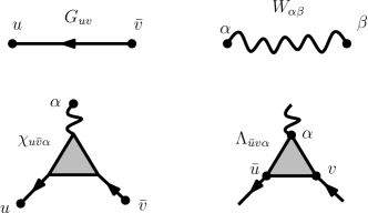
Figure 2: Graphical representation of the diagrammatic objects of the electron-boson model (Eq. 1): the fermionic propagator $G_{u\bar{v}}$ (Eq. (3c)), the bosonic propagator $W_{\alpha\beta}$ (Eq. (8)), the three-point correlation function $\chi_{u\bar{v}\alpha}$ (Eq. (13)) and the three-leg vertex $\Lambda_{\bar{u}v\alpha}$ (Eq. (15)).

II.1.2 Second Legendre transform: with respect to the three-leg vertex

We introduce the Legendre transform of $\Gamma_{2}$ with respect to $\lambda$:

$$\Gamma_{3}[\varphi,G,W,\chi^{\mathrm{nc}}]\equiv\Gamma_{2}[\varphi,G,W,\lambda]+\lambda_{\bar{v}u\alpha}\chi_{u\bar{v}\alpha}^{\mathrm{nc}}$$ (12)

where $\chi_{u\bar{v}\alpha}^{\mathrm{nc}}$ is the three-point correlator:

$$\chi_{u\bar{v}\alpha}^{\mathrm{nc}}\equiv\langle c_{u}\bar{c}_{\bar{v}}\phi_{\alpha}\rangle=-\frac{\partial\Omega}{\partial\lambda_{\bar{v}u\alpha}}\Bigg{|}_{h,F,B}$$ (13)

We also define the connected three-point function $\chi$ and the three-leg vertex $\Lambda$ as:

$$\chi_{u\bar{v}\alpha} \equiv\langle c_{u}\bar{c}_{\bar{v}}\left(\phi_{\alpha}-\varphi_{\alpha}\right)\rangle=\chi_{u\bar{v}\alpha}^{\mathrm{nc}}+G_{u\bar{v}}\varphi_{\alpha}$$ (14)

$$\Lambda_{\bar{v}u\alpha} \equiv G_{\bar{x}u}^{-1}G_{\bar{v}w}^{-1}W_{\alpha\beta}^{-1}\chi_{w\bar{x}\beta}$$ (15)

$\Lambda$ is the amputated, connected correlation function. It is the renormalized electron-boson vertex. These objects are shown graphically in Fig. 2. $G_{\bar{u}v}^{-1}$ is a shorthand notation for $\left[G^{-1}\right]_{\bar{u}v}$.

We now define the three-particle irreducible functional $\mathcal{K}$ as:

$$\mathcal{K}[\varphi,G,W,\Lambda] \equiv \Psi[\varphi,G,W,\lambda]+\lambda_{\bar{v}u\alpha}\chi_{u\bar{v}\alpha}^{\mathrm{nc}}$$ (16)

$$-\frac{1}{2}\Lambda_{\bar{x}u\alpha}G_{w\bar{x}}G_{u\bar{v}}W_{\alpha\beta}\Lambda_{\bar{v}w\beta}$$

Note that in the right-hand site, $\lambda$ is determined by $\Lambda$, $G$, $W$ and $\varphi$ (by the Legendre construction). $\mathcal{K}$ is the generalization of the functional $\mathscr{K}^{3/2}$ introduced in Ref. de Dominicis and Martin, 1964b to mixed fermionic and bosonic fields. We will come back to its diagrammatic interpretation in the next subsection.

Differentiating $\mathcal{K}$ with respect to the three-point vertex $\Lambda$ yields $K$, the generalization of the self-energy at the three-particle irreducible level, defined as:

$$K_{\bar{v}u\alpha}\equiv-G_{\bar{x}u}^{-1}G_{\bar{v}w}^{-1}W_{\alpha\beta}^{-1}\frac{\partial\mathcal{K}}{\partial\Lambda_{\bar{x}w\beta}}$$ (17)

Figure 3: Graphical representation of the diagrammatic content of $\Lambda$.

Before proceeding with the derivation, let us first state the main results: $K$ and $\Lambda$ are related by the following relation:

$$\Lambda_{\bar{v}u\alpha}=\lambda_{\bar{v}u\alpha}+K_{\bar{v}u\alpha}$$ (18)

This is the equivalent of Dyson’s equations at the 3PI level. This relation is remarkably simple: it does not involve any inversion, contrary to the Dyson equations (9a-9b). This relation is illustrated in Figure 3.

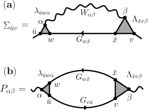
Figure 4: Graphical representation of the self-energy (beyond the Hartree term) (panel (a)) and polarization (panel (b)).

The fermionic and bosonic self-energies $\Sigma$ and $P$ are related to $\Lambda$ by the following exact relations:

$$\Sigma_{\bar{u}v} = -\lambda_{\bar{u}w\alpha}G_{w\bar{x}}W_{\alpha\beta}\Lambda_{\bar{x}v\beta}+\lambda_{\bar{u}v\alpha}\varphi_{\alpha}$$ (19a)

$$P_{\alpha\beta} = \lambda_{\bar{u}w\alpha}G_{v\bar{u}}G_{w\bar{x}}\Lambda_{\bar{x}v\beta}$$ (19b)

The second term in $\Sigma$ is nothing but the Hartree contribution. These expressions will be derived later. The graphical representation of these equations is shown in Figure 4.

II.1.3 Discussion

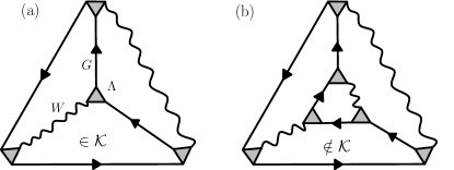
Figure 5: Three-particle irreducibility (a) Simplest contribution to the 3PI functional $\mathcal{K}$ (b) an example of diagram not contributing to $\mathcal{K}$.

The above equations, Eqs (17-18-19a-19b-9a-9b), form a closed set of equations for $G$, $W$, $\Lambda$, $\Sigma$, $P$ and $K$. The central quantity is the three-particle irreducible functional $\mathcal{K}[G,W,\Lambda]$, obtained from the 2PI functional algebraically by a Legendre transformation with respect to the bare vertex $\lambda$, or diagrammatically by a ’boldification’ of the bare vertex.

$\mathcal{K}$ has been shown to be made up of all three-particle irreducible (3PI) diagrams by de Dominicis and Martinde Dominicis and Martin (1964b) in the bosonic case. A 3PI diagram is defined as follows: for any set of three lines whose cutting leads to a separation of the diagram in two parts, one and only one of those parts is a simple three-leg vertex $\Lambda$. The simplest 3PI diagram is shown in Fig. 5(a). Conversely, neither diagram (b) of Fig. 1 nor diagram (b) of Fig. 5 are 3PI diagrams.

Most importantly, the hierarchy is closed once the functional form of $\mathcal{K}$ is specified: there is no a priori need for a higher-order vertex. This contrasts with e.g. the functional renormalization group (fRGMetzner et al. (2012)) formalism (which requires the truncation of the flow equations) or the Hedin formalismHedin (1965); Aryasetiawan and Gunnarsson (1998); Aryasetiawan and Biermann (2008) which involves the four-leg vertex $\delta\Sigma/\delta G$ via the following Bethe-Salpether-like expression for $K$:

$$K=\frac{\delta\Sigma}{\delta G}GG\Lambda$$ (20)

Of course, one must devise approximation strategies for $\mathcal{K}$ in order to solve this set of equations. In particular, any approximation involving the neglect of vertex corrections, like the FLEX approximationBickers and Scalapino (1989), spin fluctuation theoryMonthoux et al. (1991); Schmalian et al. (1998); Chubukov et al. (2002), the GW approximationHedin (1965) or the Migdal-Eliashberg theory of superconductivityMigdal (1958); Eliashberg (1960) corresponds to the approximation

$$\mathcal{K}[\varphi,G,W,\Lambda]\approx 0$$ (21)

which yields, in particular, the simple one-loop form for the self-energy:

$$\Sigma_{\bar{u}v} = -\lambda_{\bar{u}w\alpha}G_{w\bar{x}}W_{\alpha\beta}\lambda_{\bar{x}v\beta}+\lambda_{\bar{u}v\alpha}\varphi_{\alpha}$$ (22a)

$$P_{\alpha\beta} = \lambda_{\bar{u}w\alpha}G_{v\bar{u}}G_{w\bar{x}}\lambda_{\bar{x}v\beta}$$ (22b)

These approximations only differ in the type of fermionic and bosonic fields in the initial action, Eq. (1): normal/superconducting fermions, bosons in the particle-hole/particle-particle sector, in the spin/charge channel…

The core idea of the DMFT and descendent methods is to make an approximation of $\Phi$ (or $\Psi$) around the atomic limit. TRILEX is a similar approximation for $\mathcal{K}$, as will be discussed in section II.3.

II.1.4 Derivation of the main equations

In this subsection, we derive Eqs (18-19a-19b). Combining (7), (12) and (16) leads to:

$$\Gamma_{3}[\varphi,G,W,\Lambda] = \Gamma_{2}\left[\varphi,G,W,\lambda=0\right]+\mathcal{K}[\varphi,G,W,\Lambda]$$ (23)

$$+\frac{1}{2}\Lambda_{\bar{x}u\alpha}G_{w\bar{x}}G_{u\bar{v}}W_{\alpha\beta}\Lambda_{\bar{v}w\beta}$$

By construction of the Legendre transform $\Gamma_{3}$ (Eq. (12)),

$$\lambda_{\bar{v}u\alpha}=\frac{\partial\Gamma_{3}}{\partial\chi_{u\bar{v}\alpha}}\Bigg{|}_{\varphi,G,W}$$

We note that at fixed $G$ and $\varphi$, this is equivalent to differentiating with respect to $\chi_{u\bar{v}\alpha}^{\mathrm{nc}}$. Using the the chain rule and then (23) and (15) to decompose both factors yields:

$$\lambda_{\bar{v}u\alpha} = \frac{\partial\Gamma_{3}}{\partial\Lambda_{\bar{x}w\beta}}\Bigg{|}_{\varphi,G,W}\frac{\partial\Lambda_{\bar{x}w\beta}}{\partial\chi_{u\bar{v}\alpha}}\Bigg{|}_{\varphi,G,W}$$

$$= \left(\frac{\partial\mathcal{K}}{\partial\Lambda_{\bar{x}w\beta}}+G_{w\bar{s}}G_{r\bar{x}}W_{\beta\gamma}\Lambda_{\bar{s}r\gamma}\right)\left(G_{\bar{v}w}^{-1}G_{\bar{x}u}^{-1}W_{\beta\alpha}^{-1}\right)$$

$$= G_{\bar{v}w}^{-1}G_{\bar{x}u}^{-1}W_{\beta\alpha}^{-1}\frac{\partial\mathcal{K}}{\partial\Lambda_{\bar{x}w\beta}}+\Lambda_{\bar{v}u\alpha}$$

Using the definition of $K_{uv\alpha}$ (Eq. (17)), this proves Eq (18).

Let us now derive Eqs (19a-19b). They are well-known from a diagrammatic point of view, but the point of this section is to derive them analytically from the properties of $\mathcal{K}$. In order to obtain the self-energy $\Sigma$, we use Eq. (10a). We first need to reexpress $\Psi$ in terms of $\mathcal{K}$ using (16): thus

$$\Psi[\varphi,G,W,\lambda] =\tilde{\Psi}[\varphi,G,W,\lambda,\Lambda]$$

$$\equiv\mathcal{K}[\varphi,G,W,\Lambda]$$

$$+\lambda_{\bar{v}u\alpha}\chi_{u\bar{v}\alpha}^{\mathrm{nc}}-\frac{1}{2}\Lambda_{\bar{x}u\alpha}G_{w\bar{x}}G_{u\bar{v}}W_{\alpha\beta}\Lambda_{\bar{v}w\beta}$$

where $\Lambda$ is a function of $\varphi$, $G$, $W$, $\lambda$. Thus, Eq. (10a) becomes:

$$\Sigma_{\bar{u}v} = \frac{\partial\tilde{\Psi}[\varphi,G,W,\lambda,\Lambda]}{\partial G_{v\bar{u}}}\Bigg{|}_{\varphi,W,\lambda}$$

This derivative must be performed with care since the electron-boson vertex now appears in its interacting form $\Lambda$. This yields:

$$\Sigma_{\bar{u}v} = \frac{\partial\tilde{\Psi}}{\partial G_{v\bar{u}}}\Bigg{|}_{\varphi,W,\lambda,\Lambda}+\frac{\partial\tilde{\Psi}}{\partial\Lambda_{\bar{q}p\gamma}}\Bigg{|}_{\varphi,W,G,\lambda}\frac{\partial\Lambda_{\bar{q}p\gamma}}{\partial G_{v\bar{u}}}\Bigg{|}_{\varphi,W,\lambda}$$ (24)

The second term vanishes by construction of the Legendre transform. Indeed, using (16), (18) and (14):

$$\frac{\partial\tilde{\Psi}}{\partial\Lambda_{\bar{q}p\delta}}\Bigg{|}_{\varphi,W,G,\lambda} = \frac{\partial}{\partial\Lambda_{\bar{q}p\delta}}\Bigg{[}\mathcal{K}-\lambda_{\bar{s}r\gamma}\left(\chi_{r\bar{s}\gamma}-G_{r\bar{s}}\varphi_{\gamma}\right)$$

$$\;+\frac{1}{2}\Lambda_{\bar{x}u\alpha}G_{w\bar{x}}G_{u\bar{v}}W_{\alpha\beta}\Lambda_{\bar{v}w\beta}\Bigg{]}$$

$$= -G_{r\bar{q}}G_{p\bar{s}}W_{\gamma\delta}K_{\bar{s}r\gamma}-G_{r\bar{q}}G_{p\bar{s}}W_{\gamma\delta}\lambda_{\bar{s}r\gamma}$$

$$\;+G_{r\bar{q}}G_{p\bar{s}}W_{\gamma\delta}\Lambda_{\bar{s}r\gamma}$$

$$= 0$$

As a result,

$$\Sigma_{\bar{u}v} = \frac{\partial}{\partial G_{v\bar{u}}}\Bigg{[}\mathcal{K}-\lambda_{\bar{s}r\gamma}\left(\chi_{r\bar{s}\gamma}-G_{r\bar{s}}\varphi_{\gamma}\right)$$

$$+\frac{1}{2}\Lambda_{\bar{x}y\alpha}G_{w\bar{x}}G_{y\bar{z}}W_{\alpha\beta}\Lambda_{\bar{z}w\beta}\Bigg{]}\Bigg{|}_{\varphi,W,\lambda,\Lambda}$$

$$= \frac{\partial\mathcal{K}}{\partial G_{v\bar{u}}}-\lambda_{\bar{u}y\alpha}G_{y\bar{z}}W_{\alpha\beta}\Lambda_{\bar{z}v\beta}-\Lambda_{\bar{u}y\alpha}G_{y\bar{z}}W_{\beta\alpha}\lambda_{\bar{z}v\beta}$$

$$+\lambda_{\bar{u}v\alpha}\varphi_{\alpha}+\Lambda_{\bar{u}y\alpha}G_{y\bar{z}}W_{\alpha\beta}\Lambda_{\bar{z}v\beta}$$

Finally, using (18), we obtain:

$$\Sigma_{\bar{u}v} = -\lambda_{\bar{u}w\alpha}G_{w\bar{x}}W_{\alpha\beta}\Lambda_{\bar{x}v\beta}+\lambda_{\bar{v}u\alpha}\varphi_{\alpha}$$

$$+\left[\frac{\partial\mathcal{K}}{\partial G_{v\bar{u}}}+\Lambda_{\bar{u}w\alpha}G_{w\bar{x}}W_{\alpha\beta}K_{\bar{x}v\beta}\right]$$

Similarly, using (10b), one gets for $P$:

$$P_{\alpha\beta} = -2\frac{\partial\tilde{\Psi}[\varphi,G,W,\lambda,\Lambda]}{\partial W_{\beta\alpha}}\Bigg{|}_{\varphi,G,\lambda,\Lambda}$$

$$= -2\frac{\partial}{\partial W_{\beta\alpha}}\Bigg{[}\mathcal{K}-\lambda_{\bar{s}r\gamma}\left(\chi_{r\bar{s}\gamma}-G_{r\bar{s}}\varphi_{\gamma}\right)$$

$$+\frac{1}{2}\Lambda_{\bar{x}y\delta}G_{w\bar{x}}G_{y\bar{z}}W_{\delta\gamma}\Lambda_{\bar{z}w\gamma}\Bigg{]}\Bigg{|}_{\varphi,G,\lambda,\Lambda}$$

$$= -2\frac{\partial\mathcal{K}}{\partial W_{\beta\alpha}}+2\lambda_{\bar{u}w\alpha}G_{v\bar{u}}G_{w\bar{x}}\Lambda_{\bar{x}v\beta}$$

$$-\Lambda_{\bar{u}w\alpha}G_{v\bar{u}}G_{w\bar{x}}\Lambda_{\bar{x}v\beta}$$

Thus, using (18), we get

$$P_{\alpha\beta} = \lambda_{\bar{u}w\alpha}G_{v\bar{u}}G_{w\bar{x}}\Lambda_{\bar{x}v\beta}$$

$$-\left[2\frac{\partial\mathcal{K}}{\partial W_{\beta\alpha}}+K_{\bar{u}w\alpha}G_{v\bar{u}}G_{w\bar{x}}\Lambda_{\bar{x}v\beta}\right]$$

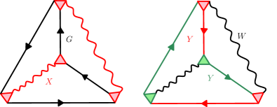
Figure 6: (color online) Homogeneity properties of the simplest diagram of $\mathcal{K}$. Left: dependence on $X$ (red). Right: dependence on $Y$ (red and green). The lines are defined in Fig. 2

Let now prove that the bracketed terms in Eqs (II.1.4-II.1.4) vanish. We first note from the diagrammatic interpretation of $\mathcal{K}$ that $\mathcal{K}$ is a homogeneous function of

$$Y_{uw\alpha} \equiv G_{w\bar{v}}\Lambda_{\bar{v}u\alpha}$$ (27a)

$$X_{u\bar{p}w\bar{z}} \equiv \Lambda_{\bar{p}u\alpha}W_{\alpha\beta}\Lambda_{\bar{z}w\beta}$$ (27b)

i.e. $\mathcal{K}$ can be written as:

$$\mathcal{K} = f_{1}(Y_{uw\alpha},W_{\alpha\beta})$$ (28a)

$$\mathcal{K} = f_{2}(X_{u\bar{p}w\bar{z}},G_{u\bar{v}})$$ (28b)

where $f_{1}$ and $f_{2}$ are two functions. This is illustrated in Fig. 6 for the simplest diagram of $\mathcal{K}$.

From (28a), one gets:

$$\frac{\partial\mathcal{K}}{\partial G_{x\bar{y}}}G_{x\bar{z}} = \Lambda_{\bar{y}u\alpha}G_{w\bar{z}}\frac{\partial f_{1}}{\partial Y_{uw\alpha}}$$ (29a)

$$\Lambda_{\bar{y}x\alpha}\frac{\partial\mathcal{K}}{\partial\Lambda_{\bar{z}x\alpha}} = \Lambda_{\bar{y}u\alpha}G_{w\bar{z}}\frac{\partial f_{1}}{\partial Y_{uw\alpha}}$$ (29b)

From (28b), in turn, one gets:

$$\Lambda_{\bar{x}v\delta}\frac{\partial\mathcal{K}}{\partial\Lambda_{\bar{x}v\gamma}} = \Lambda_{\bar{x}v\delta}\Bigg{(}W_{\gamma\beta}\Lambda_{\bar{z}w\beta}\frac{\partial f_{2}}{\partial X_{v\bar{x},w\bar{z}}}$$ (30a)

$$+\Lambda_{\bar{p}u\alpha}W_{\alpha\gamma}\frac{\partial f_{2}}{\partial X_{u\bar{p},v\bar{x}}}\Bigg{)}$$

$$= 2\Lambda_{\bar{x}v\delta}W_{\alpha\gamma}\Lambda_{\bar{p}u\alpha}\left(\frac{\partial f_{2}}{\partial X_{v\bar{x},u\bar{p}}}\right)$$

$$\frac{\partial\mathcal{K}}{\partial W_{\delta\mu}}W_{\mu\gamma} = \Lambda_{\bar{x}v\delta}W_{\alpha\gamma}\Lambda_{\bar{p}u\alpha}\frac{\partial f_{2}}{\partial X_{v\bar{x},u\bar{p}}}$$ (30b)

where we have used the property that $W$ is symmetric twice: first by trivially using $W_{\alpha\beta}=W_{\beta\alpha}$, and second to prove that

$$\frac{\partial f_{2}}{\partial X_{v\bar{x},u\bar{p}}}=\frac{\partial f_{2}}{\partial X_{u\bar{p},v\bar{x}}}$$

This latter property can be proven by noticing that when $W$ is symmetric, $f_{2}$ is a homogeneous function of the symmetrized $X$: $f_{2}(X_{AB})=\tilde{f}_{2}\left(X_{AB}^{s}\right)$, with $A=(v,\bar{x})$, $B=(u,\bar{p})$, and $X_{AB}^{s}\equiv\frac{1}{2}\left[X_{AB}+X_{BA}\right]$. Then, one has $\frac{\partial f_{2}}{\partial X_{CD}}=\frac{1}{2}\left(\delta_{CA}\delta_{DB}+\delta_{CB}\delta_{DA}\right)\frac{\partial\tilde{f}_{2}}{\partial X_{AB}^{s}}=\frac{\partial f_{2}}{\partial X_{DC}}$.

We thus obtain the following relations:

$$\frac{\partial\mathcal{K}}{\partial G_{v\bar{u}}}G_{v\bar{r}} = \Lambda_{\bar{u}w\alpha}\frac{\partial\mathcal{K}}{\partial\Lambda_{\bar{r}w\alpha}}$$ (31a)

$$2\frac{\partial\mathcal{K}}{\partial W_{\beta\alpha}}W_{\alpha\delta} = \frac{\partial\mathcal{K}}{\partial\Lambda_{\bar{x}v\delta}}\Lambda_{\bar{x}v\beta}$$ (31b)

Right-multiplying (31a) by $G^{-1}$ and (31b) by $W^{-1}$ and replacing $\partial\mathcal{K}/\partial\Lambda$ using the definition of $K$ (Eq. (17)) shows that the bracketed terms in Eqs (II.1.4-II.1.4) vanish. Thus, these expressions simplify to the final expressions for the self-energy and polarization, Eqs (19a-19b).

Finally, these exact expressions can be derived in alternative fashion using equations of motion, as shown in Appendix D.

II.2 Transposition to electron-electron problems

In this section, we show how the formalism described above can be used to study electron-electron interaction problems. We shall focus on the two-dimensional Hubbard model, which reads:

$$H=\sum_{\mathbf{RR^{\prime}}\sigma}t_{\mathbf{RR^{\prime}}}c_{\mathbf{R}\sigma}^{\dagger}c_{\mathbf{R^{\prime}}\sigma}+U\sum_{\mathbf{R}}n_{\mathbf{R}\uparrow}n_{\mathbf{R}\downarrow}$$ (32)

$\mathbf{R}$ denotes a point of the Bravais lattice, $\sigma=\uparrow,\downarrow$, $t_{\mathbf{R}\mathbf{R^{\prime}}}$ is the tight-binding hopping matrix (its Fourier transform is $\varepsilon(\mathbf{k})$), $U$ is the local Hubbard repulsion, $c_{\mathbf{R}\sigma}^{\dagger}$ and $c_{\mathbf{R}\sigma}$ are creation and annihilation operators, $n\equiv n_{\uparrow}+n_{\downarrow}$, with $n_{\sigma}=c_{\sigma}^{\dagger}c_{\sigma}$. In the path-integral formalism, the corresponding action reads:

$$S_{\mathrm{ee}}=\bar{c}_{\bar{u}}\left[-G_{0}^{-1}\right]_{\bar{u}v}c_{v}+Un_{\mathbf{R}\uparrow\tau}n_{\mathbf{R}\downarrow\tau}$$ (33)

Here, $G_{0,\sigma}^{-1}(\mathbf{k},i\omega)=i\omega+\mu-\varepsilon(\mathbf{k})$, where $i\omega$ denotes fermionic Matsubara frequencies, $\mu$ the chemical potential and the bare dispersion reads $\varepsilon(\mathbf{k})=2t\left(\cos(k_{x})+\cos(k_{y})\right)$ in the case of nearest-neighbor hoppings. $\overline{c}_{u}$ and $c_{u}$ are Grassmann fields. We remind that $u=(\mathbf{R},\tau,\sigma)$.

The Hubbard interaction in Eq. (33) can be decomposed in various ways. Defining $s^{I}\equiv\bar{c}_{u}\sigma_{uv}^{I}c_{v}$ (where $\sigma^{0}=\mathbf{1}$ and $\sigma^{x/y/z}$ denotes the Pauli matrices), the following expressions hold, up to a density term:

$$Un_{\uparrow}n_{\downarrow} =\frac{1}{2}U^{\mathrm{ch}}nn+\frac{1}{2}U^{\mathrm{sp}}s^{z}s^{z}$$ (34a)

$$Un_{\uparrow}n_{\downarrow} =\frac{1}{2}\tilde{U}^{\mathrm{ch}}nn+\frac{1}{2}\tilde{U}^{\mathrm{sp}}\vec{s}\cdot\vec{s}$$ (34b)

with the respective conditions:

$$U =U^{\mathrm{ch}}-U^{\mathrm{sp}}$$ (35a)

$$U =\tilde{U}^{\mathrm{ch}}-3\tilde{U}^{\mathrm{sp}}$$ (35b)

In Eq. (34a), the Hubbard interaction is decomposed on the charge and longitudinal spin channel (“Ising”, or “$z$”-decoupling), while in Eq. (34b) it is decomposed on the charge and full spin channel (“Heisenberg”, or “$xyz$”-decoupling). The Heisenberg decoupling preserves rotational invariance, contrary to the Ising one. In addition to this freedom of decomposition comes the choice of the ratio of the charge to the spin channel, which is encoded in Eqs. (35a-35b).

The two equalities (34a-34b) can be derived by writing that for any value of the unspecified parameters $U^{\mathrm{ch}}$ and $U^{\mathrm{sp}}$:

$$\frac{1}{2}\left(U^{\mathrm{ch}}nn+U^{\mathrm{sp}}s^{z}s^{z}\right) =\frac{1}{2}U^{\mathrm{ch}}\left(n_{\uparrow}+n_{\downarrow}\right)^{2}$$

$$\;\;+\frac{1}{2}U^{\mathrm{sp}}\left(n_{\uparrow}-n_{\downarrow}\right)^{2}$$

$$=\left(n_{\uparrow}n_{\downarrow}+\frac{n}{2}\right)(U^{\mathrm{ch}}-U^{\mathrm{sp}})$$

where we have used: $n_{\sigma}^{2}=n_{\sigma}$. Similarly, we can write:

$$\frac{1}{2}\tilde{U}^{\mathrm{ch}}nn+\frac{1}{2}\tilde{U}^{\mathrm{sp}}\vec{s}\cdot\vec{s} = \frac{1}{2}\bar{c}_{u}c_{v}\bar{c}_{w}c_{l}\delta_{uv}\delta_{wl}\tilde{U}^{\mathrm{ch}}$$

$$+\frac{1}{2}\bar{c}_{u}c_{v}\bar{c}_{w}c_{l}\left(2\delta_{ul}\delta_{vw}-\delta_{uv}\delta_{wl}\right)\tilde{U}^{\mathrm{sp}}$$

$$= \frac{1}{2}\bar{c}_{u}c_{u}\bar{c}_{v}c_{v}\tilde{U}^{\mathrm{ch}}$$

$$+\frac{1}{2}\left(2\bar{c}_{u}c_{v}\bar{c}_{v}c_{u}-\bar{c}_{u}c_{u}\bar{c}_{v}c_{v}\right)\tilde{U}^{\mathrm{sp}}$$

$$= \left(n_{\uparrow}n_{\downarrow}+\frac{n}{2}\right)(\tilde{U}^{\mathrm{ch}}-3\tilde{U}^{\mathrm{sp}})$$

Based on Eq.(35b-35a), the ratio of the bare interaction in the charge and spin channels may be parametrized by a number $\alpha$. In the Heisenberg decoupling,

$$\tilde{U}^{\mathrm{ch}} = (3\alpha-1)U$$ (36a)

$$\tilde{U}^{\mathrm{sp}} = \left(\alpha-\nicefrac{{2}}{{3}}\right)U$$ (36b)

In the Ising decoupling,

$$U^{\mathrm{ch}} = \alpha U$$ (37a)

$$U^{\mathrm{sp}} = \left(\alpha-1\right)U$$ (37b)

In the following, we adopt a more compact and general notation for Eqs (34a-34b), namely we write the interacting part of the action as:

$$S_{\mathrm{int}} = \frac{1}{2}U_{\alpha\beta}n_{\alpha}n_{\beta}$$ (38)

with

$$n_{\alpha}\equiv\bar{c}_{\bar{u}}\lambda_{\bar{u}v\alpha}c_{v}$$ (39)

We remind that $u=(\mathbf{R},\tau,\sigma)$ and $\alpha=(\mathbf{R},\tau,I)$. The parameter $I$ may take the values $I=0,x,y,z$ (Heisenberg decoupling) or a subset thereof (e.g $I=0,z$ for the Ising decoupling).

In the Hubbard model (Eq.(32)),

$$\lambda_{uv\alpha}\equiv\sigma_{\sigma_{u}\sigma_{v}}^{I}\delta_{\mathbf{R}_{u}-\mathbf{R}_{v}}\delta_{\mathbf{R}_{v}-\mathbf{R}_{\alpha}}\delta_{\tau_{u}-\tau_{v}}\delta_{\tau_{v}-\tau_{\alpha}}$$ (40)

and

$$U_{\alpha\beta}=U^{I_{\alpha}}\delta_{I_{\alpha}I_{\beta}}\delta_{\mathbf{R_{\alpha}-R_{\beta}}}\delta_{\tau_{\alpha}-\tau_{\beta}}$$ (41)

In the paramagnetic phase, one can define $U^{0}\equiv U^{\mathrm{ch}}$ and $U^{x}=U^{y}=U^{z}\equiv U^{\mathrm{sp}}$, which gives back Eqs. (34a-34b).

We now decouple the interaction (38) with a real bosonic Hubbard-Stratonovich field $\phi_{\alpha}$:

$$e^{-\frac{1}{2}U_{\alpha\beta}\left(\bar{c}_{\bar{u}}\lambda_{\bar{u}v\alpha}c_{v}\right)\left(\bar{c}_{\bar{w}}\lambda_{\bar{w}x\beta}c_{x}\right)}$$

$$=\int\mathcal{D}\left[\phi\right]e^{-\frac{1}{2}\phi_{\alpha}\left[-U^{-1}\right]_{\alpha\beta}\phi_{\alpha}\pm\lambda_{\bar{u}v\alpha}\phi_{\alpha}\bar{c}_{\bar{u}}c_{v}}$$ (42)

We have thus cast the electron-electron interaction problem in the form of Eq. (1), namely an electron-boson coupling problem. We can therefore apply the formalism developed in the previous section to the Hubbard model and similar electronic problems. The only caveat resides with the freedom in choosing the electron-boson problem for a given electronic problem: we discuss this at greater length in subsection II.3.4.

For later purposes, let us now specify the equations presented in the previous section for the Hubbard model in the normal, paramagnetic case.

In the absence of symmetry breaking,

$$G_{uv} =G_{i_{u}i_{v}}\delta_{\sigma_{u}\sigma_{v}}$$ (43)

$$W_{\alpha\beta} =W_{i_{\alpha}i_{\beta}}^{\eta(I_{\alpha})}\delta_{I_{\alpha}I_{\beta}}$$ (44)

with $i_{u}=\left(\mathbf{R}_{u},\tau_{u}\right)$, and $\eta(0)\equiv\mathrm{ch}$, $\eta(x)=\eta(y)=\eta(z)\equiv\mathrm{sp}$. In particular, $W^{0}\equiv W^{\mathrm{ch}}$ and $W^{x}=W^{y}=W^{z}\equiv W^{\mathrm{sp}}$. The vertex can be parametrized as:

$$\Lambda_{\bar{u}v\alpha}=\Lambda_{i_{u}i_{v}i_{\alpha}}^{\eta(I_{\alpha})}\sigma_{\sigma_{u}\sigma_{v}}^{I_{\alpha}}$$ (45)

$\Lambda_{ijk}^{\mathrm{ch}}$ and $\Lambda_{ijk}^{\mathrm{sp}}$ can thus be computed e.g. from

$$\Lambda_{ijk}^{\mathrm{ch}} =\Lambda_{i\uparrow,j\uparrow,k0}$$ (46a)

$$\Lambda_{ijk}^{\mathrm{sp}} =\Lambda_{i\uparrow,j\uparrow,kz}$$ (46b)

Hence, in the Heisenberg decoupling, Eqs (19a-19b) simplify to (as shown in Appendix E.1):

$$\Sigma_{ij} =-G_{il}W_{in}^{\mathrm{ch}}\Lambda_{ljn}^{\mathrm{ch}}-3G_{il}W_{in}^{\mathrm{sp}}\Lambda_{ljn}^{\mathrm{sp}}+\varphi_{j,\mathrm{ch}}\delta_{ij}$$ (47a)

$$P_{mn}^{\eta} =2G_{ml}G_{jm}\Lambda_{ljn}^{\eta}$$ (47b)

We recall that the latin indices $i,j\dots$ stand for space-time indices: $i=\left(\mathbf{R},\tau\right)$. The factor of 3 in the self-energy comes from the rotation invariance, while the factor of 2 in the polarization comes from the spin degree of freedom. Note that $\varphi_{\mathrm{ch}}$ can be related to $\langle n\rangle$ via (see Appendix B, Eq. (87a)):

$$\varphi_{\mathrm{ch}}=U^{\mathrm{ch}}\langle n\rangle$$ (48)

This is the Hartree term. In the following, we shall omit this term in the expressions for $\Sigma$ as it can be absorbed in the chemical potential term.

II.3 A local approximation to $\mathcal{K}$

In this subsection, we introduce an approximation to $\mathcal{K}$ for the specific case discussed in the previous subsection (subsection II.2).

II.3.1 The TRILEX approximation

The functional derivation discussed in subsection II.1 suggests a natural extension of the local approximations on the 2PI functionals $\Phi$ (DMFT) or $\Psi$ (EDMFT) to the 3PI functional $\mathcal{K}$. Such an approximation reads, in the case when $\mathcal{K}$ is considered as functional of $\chi_{uv\alpha}$ (instead of $\Lambda_{uv\alpha}$):

$$\mathcal{K}^{\mathrm{TRILEX}}[G,W,\chi]\approx\sum_{\mathbf{R}}\mathcal{K}[G_{\mathbf{RR}},W_{\mathbf{RR}},\chi_{\mathbf{RRR}}]$$ (49)

The TRILEX functional thus contains only local diagrams. This approximation is exact in two limits:

• in the atomic limit, all correlators become local and thus $\mathcal{K}[G_{\mathbf{RR^{\prime}}},W_{\mathbf{RR^{\prime}}},\chi_{\mathbf{RR^{\prime}R^{\prime\prime}}}]=\mathcal{K}[G_{\mathbf{RR}},W_{\mathbf{RR}},\chi_{\mathbf{RRR}}]=\mathcal{K}^{\mathrm{TRILEX}}[G,W,\chi]$;

• in the weak-interaction limit, $W$ becomes small and thus $\mathcal{K}\approx 0$, corresponding to the absence of vertex corrections and thus to the spin-fluctuation approximation.

The local approximation of the 3PI functional leads to a local approximation of the 3PI analog of the self-energy, $K$ (defined in Eq. (17)). Indeed, noticing that $\partial\mathcal{K}/\partial\chi_{vu\alpha}=K_{vu\alpha}$, Eq. (49) leads to:

$$K(\mathbf{k},\mathbf{q},i\omega,i\Omega)\approx K(i\omega,i\Omega)$$ (50)

As in DMFT, we will use an effective impurity model as an auxiliary problem to sum these local diagrams. Its fermionic Green’s function, bosonic Green’s function and three-point function are denoted as $G_{\mathrm{imp}}(i\omega)$, $W_{\mathrm{imp}}(i\Omega)$ and $\chi_{\mathrm{imp}}(i\omega,i\Omega)$ respectively. The action of the auxiliary problem is chosen such that $\mathcal{K}^{\mathrm{imp}}[G_{\mathrm{imp}},W_{\mathrm{imp}},\chi_{\mathrm{imp}}]$ is equal (up to a factor equal to the number of sites) to $\mathcal{K}^{\mathrm{TRILEX}}$ evaluated for :

$$\chi_{\mathbf{R}\mathbf{R}\mathbf{R}}^{\eta}(i\omega,i\Omega) = \chi_{\mathrm{imp}}^{\eta}(i\omega,i\Omega)$$ (51a)

$$G_{\mathrm{\mathbf{R}\mathbf{R}}}(i\omega) = G_{\mathrm{imp}}(i\omega)$$ (51b)

$$W_{\mathrm{\mathbf{R}\mathbf{R}}}^{\eta}(i\Omega) = W_{\mathrm{imp}}^{\eta}(i\Omega)$$ (51c)

This prescription, by imposing that the diagrams of the impurity model have the same topology as the diagrams corresponding to the lattice action, sets the form of impurity action as follows:

$$S_{\mathrm{imp}} = \iint_{\tau\tau^{\prime}}\sum_{\sigma}\bar{c}_{\sigma\tau}\left[-\mathcal{G}^{-1}(\tau-\tau^{\prime})\right]c_{\sigma\tau^{\prime}}$$

$$+\frac{1}{2}\iint_{\tau\tau^{\prime}}\phi_{I\tau}\left[-\left[\mathcal{U}^{I}\right]^{-1}(\tau-\tau^{\prime})\right]\phi_{I\tau^{\prime}}$$

$$+\iiint_{\tau\tau^{\prime}\tau^{\prime\prime}}\lambda_{\mathrm{imp},\sigma\sigma^{\prime}}^{I}(\tau-\tau^{\prime},\tau^{\prime}-\tau^{\prime\prime})\bar{c}_{\sigma\tau}c_{\sigma\tau^{\prime}}\phi_{I\tau^{\prime\prime}}$$

The three self-consistency equations (51a-51b-51c) completely determine the dynamical mean fields $\mathcal{G}(\tau)$, $\mathcal{U}(\tau)$ and $\lambda_{\mathrm{imp}}(\tau,\tau^{\prime})$. Note that the bare vertex $\lambda_{\mathrm{imp}}(\tau,\tau^{\prime})$ of the impurity problem is a priori different from $\lambda$, the lattice’s bare vertex, and is a priori time-dependent. Indeed, in addition to the two baths $\mathcal{G}$ and $\mathcal{U}$ present in (extended) DMFT, one needs a third adjustable quantity (akin to a Lagrange multiplierGeorges (2004)) in the impurity model to enforce the third constraint, (51a). This third Weiss field is a time-dependent electron-boson interaction. As for DMFT, the existence of Weiss fields fulfilling (51a-51b-51c) is not obvious from a mathematical point of view. In practice, we will try to construct such a model by solving iteratively the TRILEX equations.

A direct consequence of Eq. (50) and (51a-51b-51c) is the locality of the lattice vertex:

$$\Lambda^{\eta}(\mathbf{k},\mathbf{q},i\omega,i\Omega)=\lambda^{\eta}+K_{\mathrm{imp}}^{\eta}(i\omega,i\Omega)$$ (53)

where the three-particle irreducible vertex $K_{\mathrm{imp}}^{\eta}(i\omega,i\Omega)$ is related to $\Lambda_{\mathrm{imp}}^{\eta}(i\omega,i\Omega)$ through (see Eq. (18)),

$$\Lambda_{\mathrm{imp}}^{\eta}(i\omega,i\Omega)=\lambda_{\mathrm{imp}}^{\eta}(i\omega,i\Omega)+K_{\mathrm{imp}}^{\eta}(i\omega,i\Omega)$$ (54)

II.3.2 Equation for the impurity bare vertex

In TRILEX, the impurity’s bare vertex $\lambda_{\mathrm{imp}}^{\eta}(\tau,\tau^{\prime})$ is a priori different from $\lambda^{\eta}$, the bare vertex of the lattice problem. Like $\mathcal{G}(i\omega)$ and $\mathcal{U}(i\Omega)$ in EDMFT, it must be determined self-consistently. This can be contrasted with D$\Gamma$A where the bare vertex of the impurity is not renormalized and kept equal to the lattice’s bare vertex, $U$.

Let us now determine the equation for $\lambda_{\mathrm{imp}}$. Using Eq. (51a) and (15), $\Lambda_{\mathrm{imp}}$ is given by

$$\Lambda_{\mathrm{imp}}^{\eta}(i\omega,i\Omega)=\frac{\sum_{\mathbf{kq}}\chi^{\eta}(\mathbf{k},\mathbf{q},i\omega,i\Omega)}{G_{\mathrm{imp}}(i\omega+i\Omega)G_{\mathrm{imp}}(i\omega)W_{\mathrm{imp}}^{\eta}(i\Omega)}$$

$\chi^{\eta}(\mathbf{k},\mathbf{q},i\omega,i\Omega)$ is given as function of $K_{\mathrm{imp}}^{\eta}(i\omega,i\Omega)$ (after using Eqs. (18) and (50)), by

$$\chi_{\mathbf{k},\mathbf{q},i\omega,i\Omega}^{\eta}=G_{\mathbf{k}+\mathbf{q},i\omega+i\Omega}G_{\mathbf{k},i\omega}W_{\mathbf{q},i\Omega}^{\eta}\left(\lambda^{\eta}+K_{\mathrm{imp}}^{\eta}(i\omega,i\Omega)\right)$$

where we recall that $\lambda$ is the bare vertex on the lattice. Thus, $\lambda_{\mathrm{imp}}^{\eta}(i\omega,i\Omega)$ is found to be given, as a function of $K_{\mathrm{imp}}^{\eta}$, as:

$$\lambda_{\mathrm{imp}}^{\eta}(i\omega,i\Omega)=\lambda^{\eta}+\zeta^{\eta}(i\omega,i\Omega)\left\{\lambda^{\eta}+K_{\mathrm{imp}}^{\eta}(i\omega,i\Omega)\right\}$$ (55)

with

$$\zeta^{\eta}(i\omega,i\Omega)\equiv\frac{\sum_{\mathbf{k}\mathbf{q}}\tilde{G}_{\mathbf{k}+\mathbf{q},i\omega+i\Omega}\tilde{G}_{\mathbf{k},i\omega}\tilde{W}_{\mathbf{q},i\Omega}^{\eta}}{G_{\mathrm{imp}}(i\omega+i\Omega)G_{\mathrm{imp}}(i\omega)W_{\mathrm{imp}}^{\eta}(i\Omega)}$$ (56)

where for any $X$,

$$\tilde{X}(\mathbf{k},i\omega)\equiv X(\mathbf{k},i\omega)-X_{\mathrm{loc}}(i\omega)$$ (57)

Hence, in general, $\lambda_{\mathrm{imp}}$ is different from $\lambda$: one has to adjust the interaction of the impurity model to satisfy Eqs (51a-51b-51c).

II.3.3 A further simplification: reduction to density-density and spin-spin terms

The form (55) of the bare impurity vertex suggests a further approximation as a preliminary step before the full-fledged interaction term is taken into account, namely we take:

$$\lambda_{\mathrm{imp}}^{\eta}(i\omega,i\Omega)\approx\lambda^{\eta}$$ (58)

This approximation is justified when $\zeta^{\eta}(i\omega,i\Omega)$, defined in Eq. (56), is small. Let us already notice that $\zeta^{\eta}$ vanishes in the atomic limit (when $t\rightarrow 0$, $\tilde{G}=\tilde{W}=0$) and in the weak-coupling limit (then $W^{\eta}\rightarrow U^{\eta}$ so that $\tilde{W}^{\eta}\rightarrow 0$). A corollary of this simplification is that (using (53)):

$$\Lambda^{\eta}(\mathbf{k},\mathbf{q},i\omega,i\Omega)=\Lambda_{\mathrm{imp}}^{\eta}(i\omega,i\Omega)$$ (59)

We will check in subsection IV.1 that this approximation is in practice very accurate for the Hubbard model for the parameters we have considered.

With (58), integrating the bosonic modes leads to a fermionic impurity model with retarded density-density and spin-spin interactions:

$$S_{\mathrm{imp}} = \iint_{\tau\tau^{\prime}}\sum_{\sigma}\bar{c}_{\sigma}(\tau)\left[-\mathcal{G}^{-1}(\tau-\tau^{\prime})\right]c_{\sigma}(\tau^{\prime})$$ (60)

$$+\frac{1}{2}\iint_{\tau\tau^{\prime}}\sum_{I}n_{I}(\tau)\mathcal{U}^{I}(\tau-\tau^{\prime})n_{I}(\tau^{\prime})$$

The sum $\sum_{I}$ runs on $I=0,z$ in the Ising decoupling, and on $I=0,x,y,z$ in the Heisenberg-decoupling. We recall that $n_{x}\equiv s_{x}$, $n_{y}\equiv s_{y}$ and $n_{z}\equiv s_{z}$ have spin commutation rules, that is, in the Heisenberg decoupling, the spin part of the interactions explicitly reads

$$S_{\mathrm{int}}^{\mathrm{sp}}=\frac{1}{2}\iint_{\tau\tau^{\prime}}\mathcal{U}^{\mathrm{sp}}(\tau-\tau^{\prime})\vec{s}(\tau)\cdot\vec{s}(\tau^{\prime})$$

The TRILEX method is therefore solvable with the same tools as extended DMFT. The solution of the impurity action is elaborated on in section III. We will also explain how to compute $\Lambda_{\mathrm{imp}}$ from this purely fermionic action.

II.3.4 Choice of the decoupling channels

Due to the freedom in rewriting the interaction term, as discussed in subsection II.2, there are several possible Hubbard-Stratonovich decoupling fields. While an exact treatment of the mixed fermion-boson action (1) would lead to exact results, any approximation to the electron-boson action will lead to a priori different results depending on the choice of the decoupling. This ambiguity – called the Fierz ambiguity – has been thoroughly investigated in the literature in the pastCastellani and Castro (1979); Cornwall et al. (1974); Gomes and Lederer (1977); Hamann (1969); Hassing and Esterling (1973); Macêdo et al. (1982); Macêdo and Coutinho-Filho (1991); Schulz (1990); Schumann and Heiner (1988) and in more recent years Baier et al. (2004); Bartosch et al. (2009); Borejsza and Dupuis (2003, 2004); Dupuis (2002) in the context of functional renormalization group (fRG) methods.

There is no a priori heuristics to find an optimal decoupling without previous knowledge of the physically relevant instabilities of the system, except when it comes to symmetries. Optimally, the decoupling should fulfill the symmetry of the original Hamiltonian, for instance spin-rotational symmetry. Apart from pure symmetry reasons, in most cases of physical interest, where several degrees of freedom – charge, spin, superconducting fluctuations… – are competing with one another, many decoupling channels must be taken into account. This ambiguity can only be dispelled by an a posteriori control of the error with respect to the exact solution.

Yet, the TRILEX method can actually take advantage of this freedom to find the physically most relevant decoupling. It can be extended to cluster impurity problems in the spirit of cluster DMFT methods. By going to larger and larger cluster sizes and finding the decoupling which minimizes cluster corrections, one can identify the dominant physical fluctuations. In this perspective, the single-site TRILEX method presented here should be seen only as a starting point of a systematic cluster extension.

II.4 The TRILEX loop

In this section, we summarize the TRILEX set of equations, show how to solve it self-consistently, and finally touch on some technical details of the computation.

II.4.1 Summary of the equations

We recall the Dyson equations:

$$G(\mathbf{k},i\omega) = \frac{1}{i\omega+\mu-\varepsilon(\mathbf{k})-\Sigma(\mathbf{k},i\omega)}$$ (61a)

$$W^{\eta}(\mathbf{q},i\omega) = \frac{U^{\eta}}{1-U^{\eta}P^{\eta}(\mathbf{q},i\Omega)}$$ (61b)

They are merely are Fourier transforms of the equations (9a-9b). The relation between the bare interaction value $U^{\eta}$ on the Hubbard $U$ depends on the choice of decoupling. It has been discussed in subsection II.2.

The Weiss fields are given by:

$$\mathcal{G}(i\omega) = \left[G_{\mathrm{loc}}^{-1}(i\omega)+\Sigma_{\mathrm{loc}}(i\omega)\right]^{-1}$$ (62a)

$$\mathcal{U}^{\eta}(i\Omega) = \left[\left[W_{\mathrm{loc}}^{\eta}(i\Omega)\right]^{-1}+P_{\mathrm{loc}}^{\eta}(i\Omega)\right]^{-1}$$ (62b)

The “$\mathrm{loc}$” suffix denotes summation over the Brillouin zone.

The momentum-dependent lattice self-energies are given by (see Eqs (47a-47b)):

$$\Sigma{}_{\mathbf{k},i\omega} = -\sum_{\eta,\mathbf{q},i\Omega}m_{\eta}G{}_{\mathbf{k}+\mathbf{q},i\omega+i\Omega}W^{\eta}{}_{\mathbf{q},i\Omega}\Lambda_{\mathrm{imp}}^{\eta}{}_{i\omega,i\Omega}$$ (63a)

$$P^{\eta}{}_{\mathbf{q},i\Omega} = 2\sum_{\mathbf{k},i\omega}G{}_{\mathbf{k}+\mathbf{q},i\omega+i\Omega}G{}_{\mathbf{k},i\omega}\Lambda_{\mathrm{imp}}^{\eta}{}_{i\omega,i\Omega}$$ (63b)

$\Lambda_{\mathrm{imp}}$ is given by the solution of the impurity model, Eq.(60). The factor $m_{\eta}$ depends on the decoupling. In the case of the Heisenberg decoupling, $m_{\mathrm{sp}}=3$ and $m_{\mathrm{ch}}=1$, while in the Ising decoupling, $m_{\mathrm{sp}}=m_{\mathrm{ch}}=1$ (see subsection II.2).

II.4.2 Summary of the self-consistent loop

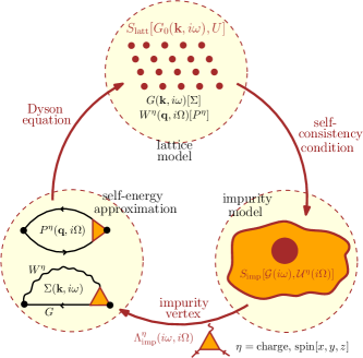
Figure 7: (color online) The TRILEX self-consistency loop

The equations above can be solved self-consistently. The self-consistent TRILEX loop consists in the following steps (as illustrated in Fig 7):

1. Initialization. The initialization consists in finding initial guesses for the self-energy and polarization. Usually, converged EDMFT self-energies provide suitable starting points for $\Sigma(\mathbf{k},i\omega)$ and $P^{\eta}(\mathbf{q},i\Omega)$.

2. Dyson equations. Compute lattice observables through Dyson equations Eqs (61a-61b).

3. Weiss fields. Update the Weiss fields using Eqs (62a-62b).

4. Impurity model. Solve the impurity action (60) for $\Lambda_{\mathrm{imp}}^{\eta}(i\omega,i\Omega)$, $\Sigma_{\mathrm{imp}}(i\omega)$ and $P_{\mathrm{imp}}(i\Omega)$

5. Self-energies. Construct momentum-dependent lattice self-energies using (63a-63b).

6. Go back to step 2 until convergence

II.4.3 Bubble with local vertices

The calculation of the self-energies (63a-63b) has to be carried out carefully for reasons of accuracy and speed.

In order to avoid the infinite summation of slowly decaying summands, we decompose (see Appendix E.2) this computation in the following way:

$$\Sigma(\mathbf{k},i\omega) = \Sigma^{\mathrm{nonloc}}(\mathbf{k},i\omega)+\Sigma_{\mathrm{imp}}(i\omega)$$ (64a)

$$P^{\eta}(\mathbf{q},i\Omega) = P^{\eta,\mathrm{nonloc}}(\mathbf{q},i\Omega)+P_{\mathrm{imp}}^{\eta}(i\Omega)$$ (64b)

with

$$\Sigma{}_{\mathbf{k},i\omega}^{\mathrm{nonloc}} \equiv -\sum_{\eta,\mathbf{q},i\Omega}m_{\eta}\tilde{G}{}_{\mathbf{k}+\mathbf{q},i\omega+i\Omega}\tilde{W}^{\eta}{}_{\mathbf{q},i\Omega}\Lambda_{\mathrm{imp}}^{\eta}{}_{i\omega,i\Omega}$$ (65a)

$$P^{\eta}{}_{\mathbf{q},i\Omega}^{\mathrm{nonloc}} \equiv \sum_{\mathbf{k},i\omega}\tilde{G}{}_{\mathbf{k}+\mathbf{q},i\omega+i\Omega}\tilde{G}{}_{\mathbf{k},i\omega}\Lambda_{\mathrm{imp}}^{\eta}{}_{i\omega,i\Omega}$$ (65b)

We also perform a further decomposition at the level of the vertex:

$$\Lambda_{\mathrm{imp}}^{\eta}(i\omega,i\Omega)=\Lambda_{\mathrm{imp}}^{\eta,\mathrm{reg}}(i\omega,i\Omega)+l^{\eta}(i\Omega)$$ (66)

where $l^{\eta}(i\Omega)\equiv\frac{1-\mathcal{\tilde{U}}^{\eta}(i\Omega)\chi_{\mathrm{imp}}^{\eta}(i\Omega)}{1-\mathcal{U}^{\eta}(i\Omega)\chi_{\mathrm{imp}}^{\eta}(i\Omega)}$, and $\tilde{\mathcal{U}}^{\eta}$ is computed with $U^{\eta}$ given by Eqs. (37a-37b) with $\alpha=1/2$. This choice corresponds to a subtraction from $\tilde{\chi}_{\mathrm{imp}}^{\eta}(i\omega,i\Omega)$ of its asymptotic behavior.

The final expressions are:

$$\Sigma(\mathbf{k},i\omega) = -\left\{\sum_{\eta,\mathbf{q},i\Omega}m_{\eta}\tilde{G}{}_{\begin{subarray}{c}\mathbf{k}+\mathbf{q}\\ i\omega+i\Omega\end{subarray}}\left[\tilde{W}_{\begin{subarray}{c}\mathbf{q}\\ i\Omega\end{subarray}}^{\eta}l_{i\Omega}^{\eta}\right]\right\}$$

$$-\sum_{\eta,\mathbf{q},i\Omega}m_{\eta}\tilde{G}_{\begin{subarray}{c}\mathbf{k}+\mathbf{q}\\ i\omega+i\Omega\end{subarray}}\tilde{W}^{\eta}{}_{\begin{subarray}{c}\mathbf{q}\\ i\Omega\end{subarray}}\left[\Lambda_{\mathrm{imp}}^{\eta,\mathrm{reg}}\right]{}_{\begin{subarray}{c}i\omega\\ i\Omega\end{subarray}}+\Sigma_{\mathrm{imp}}(i\omega)$$

$$P^{\eta}(\mathbf{q},i\Omega) = 2\left\{\sum_{\mathbf{k},i\omega}\tilde{G}_{\begin{subarray}{c}\mathbf{k}+\mathbf{q}\\ i\omega+i\Omega\end{subarray}}\tilde{G}{}_{\begin{subarray}{c}\mathbf{k}\\ i\omega\end{subarray}}\right\}l_{i\Omega}^{\eta}$$

$$+2\sum_{\mathbf{k},i\omega}\tilde{G}_{\begin{subarray}{c}\mathbf{k}+\mathbf{q}\\ i\omega+i\Omega\end{subarray}}\tilde{G}_{\begin{subarray}{c}\mathbf{k}\\ i\omega\end{subarray}}\left[\Lambda_{\mathrm{imp}}^{\eta,\mathrm{reg}}\right]_{\begin{subarray}{c}i\omega\\ i\Omega\end{subarray}}+P_{\mathrm{imp}}^{\eta}(i\Omega)$$

The first term of each expression (in curly braces) is computed as a simple product in time and space instead of a convolution in frequency and momentum. The second term, which contains factors decaying fast in frequencies ($\tilde{G}$, $\tilde{W}$, $\Lambda_{\mathrm{imp}}^{\mathrm{reg}}$), is computed as a product in space and convolution in frequencies. The spatial Fourier transforms are performed using Fast Fourier Transforms (FFT), so that the computational expense of such calculations scales as $N_{\omega}^{2}N_{k}\log N_{k}$, where $N_{\omega}$ is the number of Matsubara frequencies and $N_{k}$ the number of discrete points in the Brillouin zone.

The formulae (64a-64b) are reminiscent of the form of $\Sigma$ and $P$ in the GW+EDMFT approximation (see e.g. Ref. Ayral et al., 2013). The main difference is that in GW+EDMFT, (a) there is no local vertex correction in (65a-65b), and (b) so far GW+EDMFT has been formulated for the charge channel only.

II.4.4 Self-consistencies and alternative schemes

At this point, it should be pointed out that this choice of self-consistency conditions is not unique. In particular, inspired by the sum rules imposed in the two-particle self-consistent approximation (TPSCTremblay (2011)) or by the “Moriya corrections” of the ladder version of D$\Gamma$AKatanin et al. (2009), one may replace Eq (51c) by:

$$\chi_{\mathrm{loc}}^{\eta}(i\Omega)=\chi_{\mathrm{imp}}^{\eta}(i\Omega)$$ (69)

where $\chi^{\eta}$ (with one frequency, not to be confused with the three-point function) denotes the (connected) susceptibility in channel $\eta$:

$$\chi_{ij}^{\eta}\equiv\langle\left(n_{i}^{\eta}-\langle n_{i}^{\eta}\rangle\right)\left(n_{j}^{\eta}-\langle n_{j}^{\eta}\rangle\right)\rangle$$ (70)

This relation enforces sum rules on the double occupancy (among others) and has been shown to yield good results in the TPSC and ladder-D$\Gamma$A context, namely good agreement with exact Monte-Carlo results as well as the fulfillment of the Mermin-Wagner theorem.Vilk et al. (1994); Vilk and Tremblay (1997); Schäfer et al. (2015)

Even when using Eq (51c), however, we have shown that the sum rules are not violated for parameters where stable solutions can be obtained.Ayral and Parcollet (2015)

III Solution of the Impurity Model

The impurity model (60) with dynamical interactions in the charge and vector spin channel can be solved exactly with a continuous-time quantum Monte-Carlo (CTQMC) algorithmRubtsov et al. (2012) either in the hybridization expansion or in the interaction expansion.

In this paper, we use the hybridization expansion algorithmWerner et al. (2006); Werner and Millis (2007). Retarded vector spin-spin interactions are implemented as described in Ref. Otsuki, 2013. Our implementation is based on the TRIQS toolbox.Parcollet et al. (2015)

In this section, we give an alternative derivation of the algorithm presented in Ref. Otsuki, 2013. It uses a path integral approach, thereby allowing for a more concise presentation.

III.1 Overview of the CTQMC algorithm

Eq. (60) can be decomposed as $S_{\mathrm{imp}}=S_{\mathrm{loc}}+S_{\mathrm{hyb}}+S_{\perp}$, with:

$$S_{\mathrm{loc}} \equiv\int_{0}^{\beta}\mathrm{d}\tau\sum_{\sigma}\bar{c}_{\sigma}(\tau)\left(\partial_{\tau}-\mu\right)c_{\sigma}(\tau)$$

$$+\frac{1}{2}\iint_{0}^{\beta}\mathrm{d}\tau\mathrm{d}\tau^{\prime}\sum_{\sigma\sigma^{\prime}}n_{\sigma}(\tau)\mathcal{U}_{\sigma\sigma^{\prime}}(\tau-\tau^{\prime})n_{\sigma^{\prime}}(\tau^{\prime})$$

$$S_{\mathrm{hyb}} \equiv\int_{0}^{\beta}\mathrm{d}\tau\int_{0}^{\beta}\mathrm{d}\tau^{\prime}\sum_{\sigma}\bar{c}_{\sigma}(\tau)\Delta_{\sigma}(\tau-\tau^{\prime})c_{\sigma}(\tau^{\prime})$$

$$S_{\perp} \equiv\frac{1}{2}\iint_{0}^{\beta}\mathrm{d}t\mathrm{d}t^{\prime}\mathcal{J}_{\perp}(t-t^{\prime})s_{+}(t)s_{-}(t^{\prime})$$

where $\Delta$ is related to $\mathcal{G}$ through $\mathcal{G}_{\sigma}^{-1}(i\omega)\equiv i\omega+\mu-\Delta_{\sigma}(i\omega)$, $\mathcal{U}_{\sigma\sigma^{\prime}}(\tau)\equiv\mathcal{U}^{\mathrm{ch}}(\tau)+(-)^{\sigma\sigma^{\prime}}\mathcal{U}^{\mathrm{sp}}(\tau)$, $s_{\pm}\equiv\left(n^{x}\pm in^{y}\right)/2$, and $\mathcal{J}_{\perp}(\tau)\equiv 4\mathcal{U}^{\mathrm{sp}}(\tau)$. Note that $S_{\perp}$ is absent in the $z$-decoupling case.

We expand the partition function $Z\equiv\int\mathcal{D}[\bar{c}c]e^{-S_{\mathrm{loc}}-S_{\mathrm{hyb}}-S_{\perp}}$ in powers of $S_{\mathrm{hyb}}$ and $S_{\perp}$, which yields:

$$Z_{\mathrm{imp}}= \sum_{k_{\sigma}=0}^{\infty}\sum_{m=0}^{\infty}\int_{>}\mathrm{d}\bm{\tau}^{\sigma}\int_{>}\mathrm{d}\bm{\tau^{\prime}}^{\sigma}\int_{>}\mathrm{d}\bm{t}\int_{>}\mathrm{d}\bm{t^{\prime}}$$

$$\times \prod_{\sigma}\det\mathbf{\Delta}_{\sigma}\sum_{p\in\mathfrak{S}_{m}}\prod_{i=1}^{m}\left\{\frac{-\mathcal{J}_{\perp}(t_{p(i)}-t_{i}^{{}^{\prime}})}{2}\right\}$$

$$\times \mathrm{Tr}\left\{Te^{-S_{\mathrm{loc}}}\prod_{\sigma}\prod_{i=1}^{k_{\sigma}}c_{\sigma}(\tau_{i}^{{}^{\prime}\sigma})c_{\sigma}^{\dagger}(\tau_{i}^{\sigma})\prod_{j=1}^{m}s_{+}(t_{i})s_{-}(t_{i}^{{}^{\prime}})\right\}$$

where $k_{\sigma}$ (resp. $m$) denotes the expansion order in powers of $S_{\mathrm{hyb}}$ (resp $S_{\perp}$), $\int_{>}$ denotes integration over times sorted in decreasing order, $\bm{\tau}^{\sigma}\equiv(\tau_{1}^{\sigma}\dots\tau_{k_{\sigma}}^{\sigma})$, $\mathbf{t}\equiv(t_{1}\dots t_{m})$. Using permutations of the $c$ and $c^{\dagger}$ operators in the time-ordered product, we have grouped the hybridization terms into a determinant ($\mathbf{\Delta}_{\sigma}$ is the matrix $\left(\mathbf{\Delta}_{\sigma}\right)_{kl}\equiv\Delta_{\sigma}(\tau_{k}^{\sigma}-\tau_{l}^{{}^{\prime}\sigma})$). The term $\sum_{p\in\mathfrak{S}_{m}}\prod_{i=1}^{m}\left\{-\frac{1}{2}\mathcal{J}_{\perp}(t_{p(i)}-t_{i}^{{}^{\prime}})\right\}$ (where $\mathscr{\mathfrak{S}}_{m}$ is the group of permutations of order $m$) is the permanent of the matrix $[\tilde{\bm{\mathcal{J}}}_{\perp}]_{ij}=-\frac{1}{2}\mathcal{J}_{\perp}(t_{i}-t_{j}^{{}^{\prime}})$, but since there is no efficient way of computing the permanentValiant (1979) (contrary to the determinant), we will sample it. Finally, for any $X$, we define $\mathrm{Tr}\left[X\right]=\sum_{\bm{\gamma}}\langle\bm{\gamma}|X|\bm{\gamma}\rangle$, where $\bm{\gamma}$ is an eigenstate of the local action.

We express this multidimensional sum as a sum over configurations, namely

$$Z_{\mathrm{imp}}=\sum_{\mathscr{C}}w_{\mathscr{C}}$$ (72)

with

$$\mathscr{C}\equiv\left\{\mathbf{\bm{\tau}}^{\sigma},\mathbf{\mathbf{\bm{\tau^{\prime}}^{\sigma}}},\bm{\gamma},\mathbf{t},\mathbf{t}^{\prime},p\right\}$$ (73)

This sum is computed using Monte-Carlo sampling in the space of configurations. The weight $w_{\mathscr{C}}$ used to compute the acceptance probabilities of each Monte-Carlo update is given by:

$$w_{\mathscr{C}}=w_{\Delta}(\mathbf{\bm{\tau}}^{\sigma},\mathbf{\mathbf{\bm{\tau^{\prime}}^{\sigma}}})w_{\perp}(\mathbf{t},\mathbf{t}^{\prime},p)w_{\mathrm{loc}}(\mathbf{\bm{\tau}}^{\sigma},\mathbf{\mathbf{\bm{\tau^{\prime}}^{\sigma}}},\bm{\gamma},\mathbf{t},\mathbf{t}^{\prime})$$ (74)

with

$$w_{\Delta}(\mathbf{\bm{\tau}}^{\sigma},\mathbf{\mathbf{\bm{\tau^{\prime}}^{\sigma}}})\equiv \prod_{\sigma}\det\mathbf{\Delta}_{\sigma}$$ (75a)

$$w_{\perp}(\mathbf{t},\mathbf{t}^{\prime},p)\equiv \prod_{i=1}^{m}\left\{\frac{-\mathcal{J}_{\perp}(t_{p(i)}-t_{i}^{{}^{\prime}})}{2}\right\}$$ (75b)

$$w_{\mathrm{loc}}(\mathbf{\bm{\tau}}^{\sigma},\mathbf{\mathbf{\bm{\tau^{\prime}}^{\sigma}}},\bm{\gamma},\mathbf{t},\mathbf{t}^{\prime})\equiv \langle\bm{\gamma}|e^{-S_{\mathrm{loc}}}\prod_{\sigma}\prod_{i=1}^{k_{\sigma}}c_{\sigma}(\tau_{i}^{{}^{\prime}\sigma})\bar{c}_{\sigma}(\tau_{i}^{\sigma})$$

$$\prod_{j=1}^{m}s_{+}(t_{i})s_{-}(t_{i}^{{}^{\prime}})|\bm{\gamma}\rangle$$ (75c)

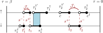
Figure 8: (color online) Pictorial representation of a Monte-Carlo configuration $\mathscr{C}$. Full (empty) circles stand for creation (annihilation) operators. The occupied portions of the imaginary time axis are represented by bold segments. The red lines represent $\mathcal{J}_{\perp}$ lines. The blue region represent an overlap between two segments.

Since the local action $S_{\mathrm{loc}}$ commutes with $n_{\sigma}$, the configuration can be represented as a collection of time-ordered “segments”Werner et al. (2006), as illustrated in Fig. 8. In this segment picture, the local weight $w_{\mathrm{loc}}$ can be simplified to:

$$w_{\mathrm{loc}}(\mathbf{\bm{\tau}}^{\sigma},\mathbf{\mathbf{\bm{\tau^{\prime}}^{\sigma}}},\bm{\gamma},\mathbf{t},\mathbf{t}^{\prime})$$

$$\;=e^{-\sum_{\sigma<\sigma^{\prime}}\overline{U}_{\sigma\sigma^{\prime}}O_{\sigma^{\prime}\sigma}(\bm{\gamma})+\bar{\mu}_{\sigma}l_{\sigma}(\bm{\gamma})}w_{\mathrm{dyn}}(\mathbf{\bm{\tau}}^{\sigma},\mathbf{\mathbf{\bm{\tau^{\prime}}^{\sigma}}},\mathbf{t},\mathbf{t}^{\prime})$$

with

$$\overline{U}_{\sigma\sigma^{\prime}} \equiv U_{\sigma\sigma^{\prime}}-2\partial_{\tau}K_{\sigma\sigma^{\prime}}(0^{+})$$

$$\bar{\mu}_{\sigma} \equiv\mu+\partial_{\tau}K_{\sigma\sigma}(0^{+})$$

The dynamical kernel $K(\tau)$ is defined as $\partial_{\tau}^{2}K_{\sigma\sigma^{\prime}}(\tau)=\mathcal{U}_{\sigma\sigma^{\prime}}(\tau)$ and $K_{\sigma\sigma^{\prime}}(0^{+})=K_{\sigma\sigma^{\prime}}(\beta^{-})=0$. $O_{\sigma\sigma^{\prime}}(\bm{\gamma})$ denotes the total overlap between lines $\sigma$ and $\sigma^{\prime}$ (blue region in Fig. 8), and $l_{\sigma}(\bm{\gamma})$ the added length of the segments of line $\sigma$. Both depend on $\bm{\gamma}$ if there are lines devoid of operators (if we note $\bm{\gamma}\equiv|n_{\uparrow},n_{\downarrow}\rangle$ in the number representation, with $n_{\sigma}=0$ or 1, whenever a “line” $\sigma$ has at least one operator, only one $n_{\sigma}$ yields a nonzero contribution, which sets its value: $n_{\sigma}$ must be specified only for lines with no operators). Finally, the contribution to the weight stemming from dynamical interactions is given by:Werner and Millis (2007)

$$\ln w_{\mathrm{dyn}}(\mathbf{\bm{\tau}}^{\sigma},\mathbf{\mathbf{\bm{\tau^{\prime}}^{\sigma}}},\mathbf{t},\mathbf{t}^{\prime}) \equiv\sum_{\begin{subarray}{c}\mathrm{ops}\\ a<b\end{subarray}}\zeta_{a}\zeta_{b}K_{\sigma_{1}(a)\sigma_{2}(b)}(\tilde{\tau}_{a}-\tilde{\tau}_{b})$$

where $\zeta_{a}$ is positive (resp. negative) if $a$ corresponds to a creation (resp. annihilation) operator, and $\tilde{\tau}$ stands for $\tau$ ($\tau^{\prime}$) for a creation (annihilation) operator. $\sum_{\begin{subarray}{c}\mathrm{ops}\\ a<b\end{subarray}}$ denotes summation over all operator pairs in a configuration (there are $\sum_{\sigma}2k_{\sigma}+4m$ such operators in a configuration).

The Monte-Carlo updates required for ergodicity in the regimes of parameters studied in this paper are (a) the insertion and removal of segments $\{c,c^{\dagger}\}$, (b) the insertion and removal of “spin” segments $\{s_{+},s_{-}\}$, (c) the permutation of the end points $\mathcal{J}_{\perp}$ lines ($p\rightarrow p^{\prime}$). They are described in more detail in Ref. Otsuki, 2013. In the insulating phase at low temperatures, an additional update consisting in moving a segment from one line to another prevents spurious spin polarizations from appearing.

In the absence of vector spin-spin interactions, the sign of a configuration is positive, i.e the sign of $w_{\mathrm{loc}}w_{\Delta}$ is positive in the absence of $s_{\pm}$ operators. The introduction of the latter does not change this statement for $w_{\mathrm{loc}}w_{\Delta}$. The sign of $w_{\mathscr{C}}$ thus reduces to that of $w_{\perp}$: from Eq. (75b), one sees that $w_{\mathscr{C}}$ is positive if and only if $\mathcal{J}_{\perp}(\tau)<0$. In practice, $\mathcal{J}_{\perp}(\tau)$ is always negative in the self-consistency introduced in subsection II.4.2. By contrast, it is usually positive for the alternative self-consistency introduced in subsection II.4.4, leading to a severe Monte-Carlo sign problem.

III.2 Computation of the vertex

The vertex is defined in Eq. (15) as the amputated, connected electron-boson correlation function $\chi(i\omega,i\Omega)$ (itself defined in Eq. (13)). Yet, since the impurity action is written in terms of fermionic variables only, $\Lambda_{\mathrm{imp}}(i\omega,i\Omega)$ is computed from the fermionic three-point correlation function $\tilde{\chi}_{\mathrm{imp}}$ through the relation (see Eqs (87b-87d) of Appendix B for a general derivation):

$$\Lambda_{\mathrm{imp}}^{\eta}(i\omega,i\Omega)$$ (76)

$$=\frac{\tilde{\chi}_{\mathrm{imp}}^{\eta}(i\omega,i\Omega)}{G_{\mathrm{imp}}(i\omega)G_{\mathrm{imp}}(i\omega+i\Omega)\left(1-\mathcal{U}^{\eta}(i\Omega)\chi_{\mathrm{imp}}^{\eta}(i\Omega)\right)}$$

where:

$$\tilde{\chi}_{\mathrm{imp}}^{\eta}(i\omega,i\Omega)\equiv\tilde{\chi}_{\mathrm{imp}}^{\eta,\mathrm{nc}}(i\omega,i\Omega)+\beta G_{\mathrm{imp}}(i\omega)\langle n_{\mathrm{imp}}^{\eta}\rangle\delta_{i\Omega}$$ (77)

where:

$$\tilde{\chi}_{\mathrm{imp}}^{\mathrm{ch},\mathrm{nc}}(i\omega,i\Omega) = \tilde{\chi}_{\mathrm{imp}}^{\uparrow\uparrow,\mathrm{nc}}(i\omega,i\Omega)+\tilde{\chi}_{\mathrm{imp}}^{\uparrow\downarrow,\mathrm{nc}}(i\omega,i\Omega)$$

$$\tilde{\chi}_{\mathrm{imp}}^{\mathrm{sp,\mathrm{nc}}}(i\omega,i\Omega) = \tilde{\chi}_{\mathrm{imp}}^{\uparrow\uparrow,\mathrm{nc}}(i\omega,i\Omega)-\tilde{\chi}_{\mathrm{imp}}^{\uparrow\downarrow,\mathrm{nc}}(i\omega,i\Omega)$$

$\tilde{\chi}_{\mathrm{imp}}^{\sigma\sigma^{\prime},\mathrm{nc}}(i\omega,i\Omega)$ is the Fourier transform of

$$\tilde{\chi}_{\mathrm{imp}}^{\sigma\sigma^{\prime},\mathrm{nc}}(\tau,\tau^{\prime})\equiv\langle Tc_{\sigma}(\tau)c_{\sigma}^{\dagger}(0)n_{\sigma^{\prime}}(\tau^{\prime})\rangle$$ (78)

(see Eq.(83a) for a definition of the Fourier transform).

The measurement of $\tilde{\chi}_{\mathrm{imp}}^{\sigma\sigma^{\prime},\mathrm{nc}}(i\omega,i\Omega)$, $G_{\mathrm{imp}}(i\omega)$ and $\chi_{\mathrm{imp}}^{\eta}(i\Omega)$ (defined in Eq. (70)) are carried out as described in Ref. Hafermann, 2014.

III.3 Computation of the self-energies

Although only the three-leg vertex $\Lambda_{\mathrm{imp}}(i\omega,i\Omega)$ is in principle required to compute the momentum-dependent self-energies through (63a-63b), the impurity self-energy and polarization may be needed for numerical stability reasons, as explained in Section II.4.3. $\Sigma_{\mathrm{imp}}(i\omega)$ is computed using improved estimators (see Ref. Hafermann, 2014), namely $\Sigma_{\mathrm{imp}}(i\omega)$ is not computed from Dyson’s equation (local version of Eq. (9a)) but using equations of motion (see Eq. (97a)). Combined with (87d) and specialized for local quantities in the paramagnetic phase, the latter equation becomes:

$$F_{\sigma,\mathrm{imp}}(\tau)=\sum_{I,\sigma^{\prime}}\sigma_{\sigma\sigma^{\prime}}^{I}\int_{0}^{\beta}d\bar{\tau}\mathcal{U}^{I}(\tau-\bar{\tau})\langle c_{\sigma^{\prime}}(\tau)\bar{c}_{\sigma}(0)n^{I}(\bar{\tau})\rangle$$

where $F_{\sigma,\mathrm{imp}}(\tau)\equiv\int d\bar{\tau}\Sigma_{\sigma,\mathrm{imp}}(\tau-\bar{\tau})G_{\sigma,\mathrm{imp}}(\bar{\tau})$. In the Ising decoupling case ($I=0,z$), this reduces to

$$F_{\sigma,\mathrm{imp}}(\tau)=\sum_{\sigma^{\prime}}\int_{0}^{\beta}d\bar{\tau}\mathcal{U}_{\sigma\sigma^{\prime}}(\tau-\bar{\tau})\langle c_{\sigma}(\tau)\bar{c}_{\sigma}(0)n_{\sigma^{\prime}}(\bar{\tau})\rangle$$ (79)

while in the Heisenberg decoupling case ($I=0,x,y,z$), one gets:

$$F_{\sigma,\mathrm{imp}}(\tau) =\int_{0}^{\beta}d\bar{\tau}\mathcal{U}^{\mathrm{ch}}(\tau-\bar{\tau})\tilde{\chi}^{\mathrm{ch}}(\tau,\bar{\tau})$$

$$+3\int_{0}^{\beta}d\bar{\tau}\mathcal{U}^{\mathrm{sp}}(\tau-\bar{\tau})\tilde{\chi}^{\mathrm{sp}}(\tau,\bar{\tau})$$ (80)

$G_{\sigma,\mathrm{imp}}(\tau)$ and $F_{\sigma,\mathrm{imp}}(\tau)$ are measured in the impurity solver, and the self-energy is finally computed as

$$\Sigma_{\sigma,\mathrm{imp}}(i\omega)=\frac{F_{\sigma,\mathrm{imp}}(i\omega)}{G_{\sigma,\mathrm{imp}}(i\omega)}$$ (81)

The polarization $P_{\mathrm{imp}}^{\eta}(i\Omega)$ is computed from the correlation function $\chi_{\mathrm{imp}}^{\eta}(i\Omega)$ by combining Eq. (87b) and the local version of (9b), i.e:

$$P_{\mathrm{imp}}^{\eta}(i\Omega)=\frac{-\chi_{\mathrm{imp}}^{\eta}(i\Omega)}{1-\mathcal{U}^{\eta}(i\Omega)\chi_{\mathrm{imp}}^{\eta}(i\Omega)}$$ (82)

IV Application to the single-band Hubbard model

In this section, we elaborate on the results presented in a prior publication (Ref. Ayral and Parcollet, 2015), where we have applied the TRILEX method in its single-site version to the single-band Hubbard model on a two-dimensional square lattice.

The main conclusions of Ref. Ayral and Parcollet, 2015 were the following:

• the TRILEX method interpolates between the spin-fluctuation regime and the Mott regime. In the intermediate regime, both the polarization and self-energy have a substantial momentum dependence.

• upon doping, one finds an important variation of the spectral weight on the Fermi surface, reminiscent of the Fermi arcs observed in angle-resolved photoemission experiments.

• the choice of the ratio of the charge to the spin channel does not significantly impact the fulfillment of sum rules on the charge and the spin susceptibility, and leads to variations only in the intermediate regime of correlations.

In the following section, we focus on four additional aspects of the method: (i) we show that the simplification of the impurity action introduced in subsection II.3.3 is justified a posteriori; (ii) we show that TRILEX has, like DMFT, a first-order Mott transition, (iii) we investigate the effect of frustration on antiferromagnetic fluctuations in the method and, (iv) we give further details on the influence of the decoupling choice.

IV.1 Check of the validity of $\lambda_{\mathrm{imp}}\approx\lambda$

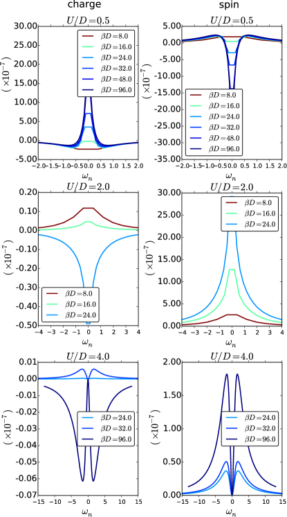
Figure 9: (color online) Evolution of $\zeta^{\eta}(i\omega_{n},i\Omega_{0})$ on the square lattice at half filling. Left column: charge channel. Right column: spin channel. From top to bottom: $U=0.5$, $U=2.0$, $U=4.0$.

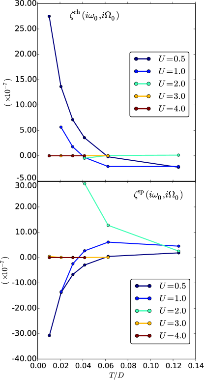
Figure 10: (color online) Dependence of $\zeta^{\eta}(i\omega_{n},i\Omega_{0})$ on temperature (square lattice, half filling). Top panel: charge channel. Bottom panel: spin channel.

The impurity action obtained after making a local expansion of the 3PI functional $\mathcal{K}$ (Eq. 49) contains a bare electron-boson vertex $\lambda_{\mathrm{imp}}(i\omega,i\Omega)$ which is a priori different from $\lambda$, the bare electron-boson vertex of the lattice action. For simplicity’s sake, we have introduced in subsection II.3.3 an additional approximation where these two vertices are regarded as equal: the general case with a frequency-dependent $\lambda_{\mathrm{imp}}(i\omega,i\Omega)$ would require an impurity solver capable of handling retarded interaction terms depending on three times (like the weak-coupling expansion solver).

The deviation between both vertices is parametrized by the function $\zeta^{\eta}(i\omega,i\Omega)$, defined in Eq. (56). For all the converged points shown in the various phase diagrams, we have checked that $\zeta^{\eta}(i\omega,i\Omega)$ remains very small, giving an a posteriori justification of our choice. This is illustrated by Figures (9) and (10).

We have also implemented an approximation where instead of neglecting the correction to $\lambda$ altogether, we replace it with $\lambda_{\mathrm{imp}}^{\eta}(i\omega_{0},i\Omega_{0})$ (and hence the interactions become $\left(\lambda_{\mathrm{imp}}^{\eta}(i\omega_{0},i\Omega_{0})\right)^{2}\mathcal{U}^{\eta}(i\Omega)$, which one can still handle with the impurity solver presented above). This, however, did not lead to any visible modification of the converged solution with respect to the simplified scheme presented throughout this paper.

IV.2 A first-order Mott transition

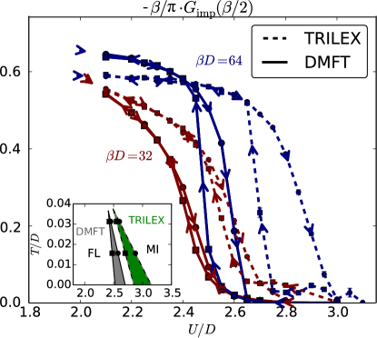
Figure 11: (color online) Evolution of $-\beta/\pi G_{\mathrm{imp}}(\tau=\beta/2)$ as a function of $U/D$ on the triangular lattice (half-filling). Solid lines: DMFT. Dashed lines: TRILEX. Red: $\beta D=32$. Blue: $\beta D=64$. Inset: sketch of the coexistence regions in DMFT (grey) and TRILEX (green) in the $(U,T)$ plane.

In Ref. Ayral and Parcollet, 2015, several points in the phase diagram have been studied. Due to very small denominators in $W^{\mathrm{sp}}(\mathbf{q},i\Omega=0)$, no stable solution could be obtained at low enough temperatures to go below the temperature of the critical end point of the Mott transition line ($T_{\mathrm{Mott}}/D\approx 0.045$ on the Bethe lattice, see e.g. Ref Vučičević et al., 2013). In this section, we turn to the triangular lattice in two dimensions and at half-filling to characterize the nature of the Mott transition. On this lattice, geometrical frustration mitigates the low-temperature instabilities, allowing to reach lower temperatures.

In Fig. 11, the evolution of $-\beta/\pi\cdot G_{\mathrm{imp}}(\tau=\beta/2)$ is monitored for two temperatures as a function of $U/D$. At low enough temperatures, $-\beta/\pi\cdot G_{\mathrm{imp}}(\tau=\beta/2)$ is an accurate estimate of $A_{\mathrm{imp}}(\omega=0)$, and can thus be used to observe the transition between a Fermi liquid ($A_{\mathrm{imp}}(\omega=0)>0$) and a Mott insulator ($A_{\mathrm{imp}}(\omega=0)\approx 0$). At low temperatures ($\beta D=64$), both DMFT and TRILEX display a hysteretic behavior, namely there is a coexistence region between a metallic and insulating solution. At a higher temperature ($\beta D=32$), the hysteretic region has shrunk. With these two estimates for $U_{c}$, one can draw a rough sketch of the $(T,U)$ phase diagram in the triangular lattice (see the inset).

From this study of TRILEX on the triangular lattice, two conclusions can be drawn: (i) TRILEX, like DMFT, features a first-order Mott transition; and (ii) in TRILEX, the critical interaction strength for the Mott transition, $U_{c}$, is slightly enhanced with respect to the single-site DMFT value. The latter observation is consistent with the difference that has been observed between the local component of the TRILEX self-energy and the single-site DMFT self-energy.Ayral and Parcollet (2015)

This observation contrasts with cluster methodsMoukouri and Jarrell (2001); Zhang and Imada (2007); Park et al. (2008) and diagrammatic extensions of DMFT like the D$\Gamma$A methodSchäfer et al. (2015) or the dual fermion methodBrener et al. (2008); Hafermann (2009). In all these methods, $U_{c}$ is strongly reduced with respect to single-site DMFT. This discrepancy possibly points to the partial neglect of short-range physics in single-site TRILEX, contrary to diagrammatic and cluster extensions of DMFT. In the former class of methods, the resummation of ladder diagrams might explain why they seem to better capture short-range processes. In the latter class of methods, short-range fluctuations are treated explicitly and non-perturbatively in the extended impurity model. This motivates the need for exploring cluster extensions of TRILEX and comparing TRILEX with D$\Gamma$A results in more detail.

IV.3 Antiferromagnetic fluctuations: influence of frustration

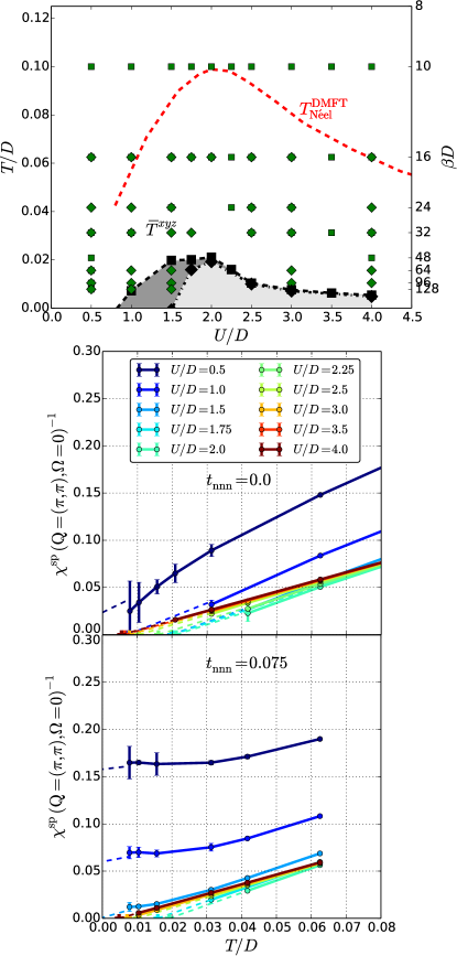
Figure 12: (color online) Influence of $t^{\prime}$ on $\overline{T}^{xyz}$ (square lattice). Phase diagram in the $(T,U$) plane at half-filling. The green squares (resp. diamonds) denote converged TRILEX calculations for $t^{\prime}=0$ (resp. $t^{\prime}=-0.3t$). The red dashed line is the Néel temperature computed in single-site DMFT (from Ref. Kuneš, 2011). In the gray regions (dark gray for $t^{\prime}=0$, light gray for $t^{\prime}=-0.3t$) at low temperatures, vanishing denominators in $W^{\mathrm{sp}}(\mathbf{q},i\Omega=0)$ preclude convergence. Bottom panels: inverse static AF susceptibility as a function of temperature for various $U/D$ values. Top: $t^{\prime}=0$. Bottom: $t^{\prime}=-0.3t$.

In this section, we investigate the effect of frustration, parametrized by a next-nearest-neighbor hopping term $t^{\prime}$, on antiferromagnetic fluctuations and on the convergence properties of the method.

The results are gathered in Fig. 12. As shown in the lowers panels, as the temperature is decreased, the strength of the antiferromagnetic fluctuations, parametrized by the static inverse antiferromagnetic susceptibility $\chi^{\mathrm{sp}}(\mathbf{Q},i\Omega=0)^{-1}$, grows, namely the product $U^{\mathrm{sp}}P^{\mathrm{sp}}(\mathbf{q},i\Omega)$ approaches the “Stoner” criterion $U^{\mathrm{sp}}P^{\mathrm{sp}}(\mathbf{q},i\Omega)=1$. In the frustrated case (lower-right panel), however, the AF spin susceptibility strongly reduced with respect to the unfrustrated case at weak values of the local interaction $U$. It is unchanged for larger interaction values. Consequently, the zone of unstable solutions (gray area in the upper panel) shrinks in the weak-interaction regime and remains unchanged in the Mott regime.

The question of the exact nature of this low-temperature phase is still open. To decide whether at low temperatures, the inverse AF susceptibility indeed intercepts the $x$-axis at a finite $T_{\mathrm{N\acute{e}el}}$, as the high-temperature behavior seems to indicate, or if it displays a bending (as observed in the correlation length in experiments – see e.g. Ref. Keimer et al., 1992 – or in theory – see e.g. Ref. Schäfer et al., 2015), requires a more refined study which is beyond the scope of this paper. The issue could e.g. be settled by allowing for a symmetry breaking with two sublattices. This idea is straightforward to implement, but requires another impurity solver, since in the AF phase the longitudinal ($z$) and perpendicular ($x,y$) spin components are no longer equivalent. In this phase, one has to measure the perpendicular components $\Lambda_{\mathrm{imp}}^{x/y}$ of the vertex instead of $\Lambda_{\mathrm{imp}}^{z}$ only.

IV.4 Ising versus Heisenberg decoupling

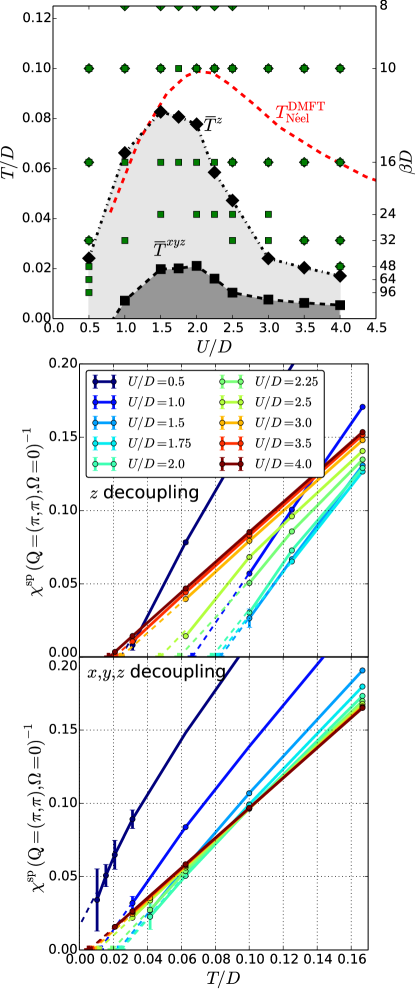
Figure 13: (color online) Top panel: Phase diagram in the $(T,U$) plane at half-filling (square lattice, $t^{\prime}=0$). The dashed red line is the Néel temperature computed in single-site DMFT (from Kuneš (2011)). Left: Heisenberg ($\overline{T}^{xyz}$) vs. Ising ($\overline{T}^{z}$) decoupling (squares: Heisenberg; diamonds: Ising). $\overline{T}$ is determined by extrapolating the inverse AF static susceptibility. Bottom panels: Inverse AF static susceptibility as a function of temperature (square lattice). Top: Ising or “$z$” decoupling. Bottom: Heisenberg or “$xyz$” decoupling

In this subsection, we discuss the practical implications of the way the Hubbard interaction term is decoupled in terms of Hubbard-Stratonovich terms.

Already at the single-site level, we have investigated the influence of the ratio of charge to spin channel and shown that it does not impact the fulfillment of sum rulesAyral and Parcollet (2015).

Here, we focus on the difference between the “Ising” and “Heisenberg” decouplings introduced in subsection II.2. We show, in Fig. 13 (upper panel), the phase diagram for both choices of decoupling. As before, the boundary of the region of unstable solutions, shown in gray, has been obtained by following the evolution of the inverse static AF susceptibility as a function of temperature for both decouplings. The extrapolated $\overline{T}$ strongly depends on the decoupling: it is much larger for the Ising decoupling than for the Heisenberg decoupling.

This can be understood in the following intuitive way: in the Ising decoupling, the spin has fewer degrees of freedom to fluctuate than in the Heisenberg decoupling. Thus, correlation lengths are much larger in the Ising decoupling than in the Heisenberg decoupling. In either case, $\overline{T}$ is lower than the Néel temperature computed in single-site DMFT (except for a few points in the Ising decoupling at weak coupling, but the difference is within error bars): TRILEX contains spatial fluctuations beyond (dynamical) mean field theory.

V Conclusions and perspectives

In this paper, we have presented the TRILEX formalism, which consists in making a local expansion of the 3PI functional $\mathcal{K}$. This approximation entails the locality of the three-leg vertex which is self-consistently computed by solving an impurity model with dynamical charge and spin interactions.

By construction, this method interpolates between two major approaches to high-temperature superconductors, namely, fluctuation-exchange approximations such as spin fluctuation theory, and dynamical mean-field theory and its cluster extensions. The central quantity of TRILEX, the impurity three-leg vertex $\Lambda_{\mathrm{imp}}(i\omega,i\Omega)$, encodes the passage from both limits. It can be used to construct momentum-dependent self-energies and polarizations at a reduced cost compared to cluster DMFT and diagrammatic extensions of DMFT. More specifically, it requires the solution of a single-site local impurity model with dynamical interactions.

Contrary to spin fluctuation theory, the method explicitly captures Mott physics via the frequency-dependent vertex. Contrary to recent diagrammatic extensions of DMFT attempting to incorporate long-range physics such as D$\Gamma$AToschi et al. (2007); Katanin et al. (2009) and the dual fermion methodRubtsov et al. (2008), it deals with functions of two (instead of three) frequencies, which makes it more easily extendable to a cluster and/or multiorbital implementation. Indeed, four-leg vertices are a major computational burden in those methods, owing to their sheer size in memory and also to the appearance of divergencies in some of these vertices already for moderate interaction valuesSchäfer et al. (2013), as well as divergencies when inverting the Bethe-Salpether equations in a given channelKatanin et al. (2009).

Here, the TRILEX method in its single-site version has been applied to the single-band Hubbard model, on the square and on the triangular lattice. As expected from the construction of the method, TRILEX interpolates between (a) the fluctuation-exchange limit, where the self-energy is given by the one-loop diagram computed with the propagator associated to long-range fluctuations in channel $\eta$, $W^{\eta}(\mathbf{q},i\Omega)$, and (b) the dynamical mean field limit which approximates the self-energy by a local, but frequency-dependent impurity self-energy which reduces, in the strong-coupling regime, to the atomic limit self-energy. At intermediate coupling, upon doping, strong AF fluctuations cause a sizable momentum differentiation of the Fermi surface, as observed in photoemission in cuprate materials.

There are many open issues:

1. Low-temperature phase. The issue of the instabilities in the low-temperature regime, which is related to the fulfillment or not of the Mermin-Wagner theorem and the associated Fierz ambiguity, deserve further studies. This is all the more interesting as related methods such as TPSC and ladder-D$\Gamma$A with the additional Moriya correction fulfill the Mermin-Wagner theorem; a better understanding of the minimal ingredients to enforce this property is needed.

2. Extension to cluster schemes. The accuracy of the TRILEX method can be assessed quantitatively by extending it to clusters. Due to the inclusion of long-range fluctuations, one may anticipate that cluster TRILEX will converge faster than cluster DMFT with respect to the cluster size $N_{c}$ in the physically relevant channel. Moreover, when convergence with respect to $N_{c}$ is reached, the results will be totally independent of the choice of channels. As a result, the channel dependence for a given cluster (e.g. a given size) is an indication of the degree of its convergence which does not necessitate the computation of larger clusters. This property has no analog in cluster DMFT methods.

3. Extension to multiorbital systems. Thanks to the simplicity of solving the single-site impurity model, single-site TRILEX can be applied to multiorbital systems to study momentum-dependent self-energy effects. Such an endeavor is currently out of the reach of cluster DMFT due to the sheer size of the corresponding Hilbert space (3 bands times a $2\times 2$ cluster is effectively a 12-site calculation, already a large numerical effort). Yet, this extension may be crucial for multiorbital systems where long-range spin physics as well as correlations are thought to play an important role. For instance, the pnictide superconductors, where bosonic spin-density-wave fluctuations are sizable but correlations effects are not so strong, may prove an ideal playing ground for TRILEX.

4. Extension to “anomalous” phases. TRILEX can be straightforwardly extended to study charge-ordered phases (as shown by its relation to $GW$+EDMFT). Moreover, its application to superconducting phases is also possible: in this context, it interpolates between generalized Migdal-Eliashberg theory (or spin-fermion superconductivity) and the superconducting version of DMFT. As such, it can capture $d$-wave superconductivity at the cost of solving a single-site impurity problem (which is not possible in single-site DMFT).

5. Nonlocal extensions. One natural route beyond the local approximation of the vertex is to construct the lattice vertex as the sum of the impurity vertex with a nonlocal diagrammatic correction, in the same way as the GW+EDMFT method extends EDMFT by adding nonlocal diagrams to the impurity self-energies.

6. Extension to the three-boson vertex. In the functional construction presented in this paper, we have only considered a three-point source term with one bosonic field and two fermionic fields. In principle, for the sake of 3PI-completeness, one could also introduce an additional three-point source term coupling three bosonic fields. We have not explored this path here since it requires an impurity solver handling both fermionic and bosonic fields.

Appendix A Symmetry Properties of the Vertex and Fourier Conventions

A.1 Fourier conventions

We follow the following Fourier conventions, depending on whether we want to work with a fermionic and a bosonic Matsubara frequency, or two fermionic frequencies:

$$A_{\mathbf{R}_{1}\mathbf{R}_{2}\mathbf{R}_{3}}(i\omega,i\Omega) \equiv \iint_{0}^{\beta}\mathrm{d}\tau\mathrm{d}\tau^{\prime}e^{i\omega\tau+i\Omega\tau^{\prime}}A_{\mathbf{R}_{1}\mathbf{R}_{2}\mathbf{R}_{3}}(\tau,0,\tau^{\prime})$$ (83a)

$$\hat{A}_{\mathbf{R}_{1}\mathbf{R}_{2}\mathbf{R}_{3}}(i\omega_{1},i\omega_{2}) \equiv \iint_{0}^{\beta}\mathrm{d}\tau\mathrm{d}\tau^{\prime}e^{i\omega_{1}\tau+i\omega_{2}\tau^{\prime}}A_{\mathbf{R}_{1}\mathbf{R}_{2}\mathbf{R}_{3}}(\tau,\tau^{\prime},0)$$ (83b)

for any three-point function $A(\mathbf{R}_{1},\tau_{1};\mathbf{R}_{2},\tau_{2};\mathbf{R}_{3},\tau_{3})$, $e.g$ $A_{\mathbf{R}_{1}\mathbf{R}_{2}\mathbf{R}_{3}}(\tau_{1},\tau_{2},\tau_{3})=\langle Tc_{\mathbf{R}_{1}}(\tau_{1})c_{\mathbf{R}_{2}}^{\dagger}(\tau_{2})\phi_{\mathbf{R}_{3}}(\tau_{3})\rangle$. Both functions are related:

$$A_{\mathbf{R}_{1}\mathbf{R}_{2}\mathbf{R}_{3}}(i\omega,i\Omega)=\hat{A}_{\mathbf{R}_{1}\mathbf{R}_{2}\mathbf{R}_{3}}(i\omega,-i\omega-i\Omega)$$ (84)

In the main text, we only use the first form $A_{\mathbf{R}_{1}\mathbf{R}_{2}\mathbf{R}_{3}}(i\omega,i\Omega)$.

A.2 Lehmann representation of the three-leg vertex

Using the identity $\int_{0}^{\beta}\int_{0}^{\beta}dt_{1}dt_{2}Tf_{1}(t_{1})f_{2}(t_{2})=\int_{0}^{\beta}\int_{0}^{t_{1}}dt_{1}dt_{2}\sum_{p\in\mathfrak{S}_{2}}\sigma(p)f_{p1}(t_{1})f_{p2}(t_{2})$, we can write, using the definition of $\tilde{\chi}$ (Eq. 88) and of its Fourier transform (Eq. 83b)

$$\hat{\tilde{\chi}}_{123}(i\omega_{1},i\omega_{2})$$

$$\equiv\sum_{p\in\mathfrak{S}_{2}}\int_{0}^{\beta}\mathrm{d}\tau\int_{0}^{\tau}\mathrm{d}\tau^{\prime}\sigma(p)\langle O_{p1}(\tau)O_{p2}(\tau^{\prime})n_{3}(0)\rangle e^{i\omega_{p1}\tau}e^{i\omega_{p2}\tau^{\prime}}$$

$$=\frac{1}{Z}\sum_{ijk}\sum_{p\in\mathfrak{S}_{2}}\sigma(p)\langle i|O_{p1}|j\rangle\langle j|O_{p2}|k\rangle\langle k|n_{3}|i\rangle f_{ijk}(\omega_{p1},\omega_{p2})$$ (85)

with $O_{1}=c_{1}^{\dagger}$ and $O_{2}=c_{2}$, and:

$$f_{ijk}(\omega_{1},\omega_{2})$$

$$=e^{-\beta\epsilon_{i}}\int_{0}^{\beta}\mathrm{d}\tau e^{\tau(i\omega_{1}+\epsilon_{i}-\epsilon_{j})}\int_{0}^{\tau}\mathrm{d}\tau^{\prime}e^{\tau^{\prime}(i\omega_{2}+\epsilon_{j}-\epsilon_{k})}$$

$$=e^{-\beta\epsilon_{i}}\int_{0}^{\beta}\mathrm{d}\tau e^{\tau(i\omega_{1}+\epsilon_{i}-\epsilon_{j})}\frac{e^{\tau(i\omega_{2}+\epsilon_{j}-\epsilon_{k})}-1}{i\omega_{2}+\epsilon_{j}-\epsilon_{k}}$$

$$=\frac{e^{-\beta\epsilon_{i}}}{i\omega_{2}+\epsilon_{j}-\epsilon_{k}}\int_{0}^{\beta}\mathrm{d}\tau\left(e^{\tau(i\omega_{1}+i\omega_{2}+\epsilon_{i}-\epsilon_{k})}-e^{\tau(i\omega_{1}+\epsilon_{i}-\epsilon_{j})}\right)$$

$$=\frac{e^{-\beta\epsilon_{i}}}{i\omega_{2}+\epsilon_{j}-\epsilon_{k}}\Bigg{(}\frac{e^{\beta(i\omega_{1}+i\omega_{2}+\epsilon_{i}-\epsilon_{k})}-1}{i\omega_{1}+i\omega_{2}+\epsilon_{i}-\epsilon_{k}}\left(1-\delta_{ik}\right)$$

$$\;\;-\frac{e^{\beta(i\omega_{1}+\epsilon_{i}-\epsilon_{j})}-1}{i\omega_{1}+\epsilon_{i}-\epsilon_{j}}\Bigg{)}+\frac{e^{-\beta\epsilon_{i}}}{i\omega_{2}+\epsilon_{j}-\epsilon_{i}}\beta\delta_{i\omega_{1}+i\omega_{2}}\delta_{ik}$$

$$=\frac{1}{i\omega_{2}+\epsilon_{j}-\epsilon_{k}}\Bigg{(}\frac{e^{-\beta\epsilon_{k}}-e^{-\beta\epsilon_{i}}}{i\omega_{1}+i\omega_{2}+\epsilon_{i}-\epsilon_{k}}\left(1-\delta_{ik}\right)$$

$$\;\;+\frac{e^{-\beta\epsilon_{j}}+e^{-\beta\epsilon_{i}}}{i\omega_{1}+\epsilon_{i}-\epsilon_{j}}\Bigg{)}+\frac{e^{-\beta\epsilon_{i}}}{i\omega_{2}+\epsilon_{j}-\epsilon_{i}}\beta\delta_{i\omega_{1}+i\omega_{2}}\delta_{ik}$$

We have used the fact that both $i\omega_{1}$ and $i\omega_{2}$ are fermionic Matsubara frequencies ($e^{\beta i\omega_{1}}=-1$).

A.3 Symmetries of the three-point vertex

In this section, we derive the main symmetries of the three-point vertex in a simple limit. We consider the most simple fermionic model, namely a single fermionic level, $O_{1}=c^{\dagger}$, $O_{2}=c$. $O_{1}^{\dagger}=O_{2}$ (in the notations of Section A.2). The Hilbert space consists in two states: $|0\rangle$ and $|1\rangle$ with respective energies $0$ and $\epsilon$. Starting from 85, we have:

$$\hat{\tilde{\chi}}(i\omega_{1},i\omega_{2}) = \frac{1}{Z}\sum_{ijk}\langle i|O_{1}|j\rangle\langle j|O_{2}|k\rangle\langle k|n|i\rangle f(\omega_{1},\omega_{2})$$

$$+\underbrace{\sum_{ijk}\langle i|O_{2}|j\rangle\langle j|O_{1}|k\rangle\langle k|n|i\rangle f(\omega_{2},\omega_{1})}_{=0}$$

$$= \frac{1}{Z}\langle 1|c^{\dagger}|0\rangle\langle 0|c|1\rangle\langle 1|n|1\rangle f(\omega_{1},\omega_{2})$$

$$= \frac{1}{Z}f_{101}(\omega_{1},\omega_{2})$$

$$= \frac{1}{Z}\frac{1}{i\omega_{2}-\epsilon}\left(\frac{1+e^{-\beta\epsilon}}{i\omega_{1}+\epsilon}\right)+\frac{1}{Z}\frac{e^{-\beta\epsilon}}{i\omega_{2}-\epsilon}\delta_{i\omega_{1}+i\omega_{2}}$$

Hence,

$$\tilde{\chi}(i\omega,i\Omega) \propto\frac{1}{-i\omega-i\Omega-\epsilon}\frac{1}{i\omega+\epsilon}+\frac{1}{-i\omega-\epsilon}\delta_{i\Omega}$$

$$\propto\frac{1}{i\omega+i\Omega+\epsilon}\frac{1}{i\omega+\epsilon}+\frac{1}{i\omega+\epsilon}\delta_{i\Omega}$$

One can notice:

$$\tilde{\chi}(i\omega-i\Omega,i\Omega) \propto\frac{1}{i\omega+\epsilon}\frac{1}{i\omega-i\Omega+\epsilon}+\frac{1}{i\omega-i\Omega+\epsilon}\delta_{i\Omega}$$

$$=\chi(i\omega,-i\Omega)$$

and:

$$\tilde{\chi}^{*}(i\omega,-i\Omega) \propto\left(\frac{1}{i\omega-i\Omega+\epsilon}\frac{1}{i\omega+\epsilon}+\frac{1}{i\omega+\epsilon}\delta_{i\Omega}\right)^{*}$$

$$=\frac{1}{-i\omega+\epsilon}\frac{1}{i\Omega-i\omega+\epsilon}+\frac{1}{-i\omega+\epsilon}\delta_{i\Omega}$$

$$=\tilde{\chi}(-i\omega,i\Omega)$$

Thus, we obtain the following symmetry relations:

$$\tilde{\chi}(i\omega-i\Omega,i\Omega) =\tilde{\chi}(i\omega,-i\Omega)$$ (86a)

$$\tilde{\chi}^{*}(i\omega,-i\Omega) =\tilde{\chi}(-i\omega,i\Omega)$$ (86b)

One can check that these symmetry relations hold in the general case and carry over to the vertex $\Lambda(i\omega,i\Omega)$. A pictorial representation of these symmetries is given in Fig. 14.

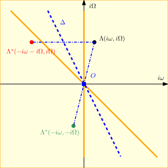
Figure 14: (color online) Vertex symmetries

Appendix B Link between bosonic correlation functions and fermionic correlation functions

In this appendix, we prove the following relations between observables of the mixed fermion-boson action (1) and observables of the fermionic action:

$$\varphi_{\alpha}^{\eta} = U_{\alpha\beta}^{\eta}\langle n_{\beta}^{\eta}\rangle$$ (87a)

$$W_{\alpha\beta}^{\eta,\mathrm{nc}} = U_{\alpha\beta}^{\eta}-U_{\alpha\gamma}^{\eta}\chi_{\gamma\delta}^{\eta,\mathrm{nc}}U_{\delta\beta}^{\eta}$$ (87b)

$$W_{\alpha\beta}^{\eta} = U_{\alpha\beta}^{\eta}-U_{\alpha\gamma}^{\eta}\chi_{\gamma\delta}^{\eta}U_{\delta\beta}^{\eta}$$ (87c)

$$\chi_{u\bar{v}\alpha}^{\eta} = U_{\alpha\beta}^{\eta}\tilde{\chi}_{u\bar{v}\beta}^{\eta}$$ (87d)

$W_{\alpha\beta}^{\eta}$, $\chi_{\alpha\beta}^{\eta}$ and $\chi_{uv\alpha}^{\eta}$ have been defined in Eqs (3b), (70) and (13) respectively, and

$$\tilde{\chi}_{u\bar{v}\alpha}^{\mathrm{nc}}\equiv\langle c_{u}\bar{c}_{\bar{v}}n_{\alpha}\rangle$$ (88)

Let us recall the definition of the partition function in the presence of sources

$$Z[h,F,B]\equiv\int\mathcal{D}[\bar{c},c,\phi]e^{-S_{\mathrm{eb}}+h_{\alpha}\phi_{\alpha}-F_{\bar{u}v}\bar{c}_{\bar{u}}c_{v}-\frac{1}{2}\phi_{\alpha}B_{\alpha\beta}\phi_{\beta}}$$ (89)

Integrating out the bosonic fields yields:

$$Z[h,F,B] =\mathrm{Det}\left[\bar{U}^{-1}\right]^{-1/2}$$ (90)

$$\;\times\int\mathcal{D}[\bar{c},c]e^{-\bar{c}_{\bar{u}}\left\{-G_{0,\bar{u}v}^{-1}+F_{\bar{u}v}\right\}c_{v}+\frac{1}{2}\bar{U}_{\alpha\beta}(h_{\alpha}-\bar{c}_{\bar{u}}\lambda_{\bar{u}v\alpha}c_{v})^{2}}$$

$$=e^{\frac{1}{2}\mathrm{Tr}\log\left[\bar{U}\right]}$$

$$\;\times\int\mathcal{D}[\bar{c},c]e^{-\bar{c}_{\bar{u}}\left\{-G_{0,\bar{u}v}^{-1}+F_{\bar{u}v}\right\}c_{v}+\frac{1}{2}\bar{U}_{\alpha\beta}(h_{\alpha}-\bar{c}_{\bar{u}}\lambda_{\bar{u}v\alpha}c_{v})^{2}}$$

with $\bar{U}_{\alpha\beta}=\left[\left(-U^{-1}+B\right)^{-1}\right]_{\alpha\beta}$. Hence

$$\Omega =\frac{1}{2}\mathrm{Tr}\log\left[-U^{-1}+B\right]$$

$$\;\;-\log\int\mathcal{D}[\bar{c},c]\Bigg{[}e^{-\bar{c}_{\bar{u}}\left\{-G_{0,\bar{u}v}^{-1}+F_{\bar{u}v}\right\}c_{v}}$$

$$\;\;\times e^{\frac{1}{2}\bar{U}_{\alpha\beta}\left(h_{\alpha}-\bar{c}_{\bar{u}}\lambda_{\bar{u}v\alpha}c_{v}\right)\left(h_{\beta}-\bar{c}_{\bar{u}}\lambda_{\bar{u}v\beta}c_{v}\right)}\Bigg{]}$$

Relation (87a) follows from computing $\varphi_{\alpha}$ by successively using (89) and (90):

$$\varphi_{\alpha}=\frac{1}{Z}\frac{\partial Z}{\partial h_{\alpha}}=U_{\alpha\beta}\langle\bar{c}_{\bar{u}}\lambda_{\bar{u}v\beta}c_{v}\rangle$$

Similarly, one has:

$$W_{\alpha\beta}^{\mathrm{nc}} = -2\frac{\partial\Omega}{\partial B_{\alpha\beta}}$$

$$= -2\left[\frac{1}{2}\left(-U_{\alpha\beta}\right)\right]$$

$$-2\left[-\frac{1}{2}\left(\frac{\partial\bar{U}_{\gamma\delta}}{\partial B_{\alpha\beta}}\right)\left(h_{\gamma}-\bar{c}_{\bar{u}}\lambda_{\bar{u}v\gamma}c_{v}\right)\left(h_{\delta}-\bar{c}_{\bar{u}}\lambda_{\bar{u}v\delta}c_{v}\right)\right]$$

$$= U_{\alpha\beta}-U_{\alpha\delta}\langle\left(\bar{c}_{u}\lambda_{\bar{u}v\delta}c_{v}\right)\left(\bar{c}_{\bar{u}}\lambda_{\bar{u}v\gamma}c_{v}\right)\rangle U_{\gamma\beta}$$

$$= U_{\alpha\beta}-U_{\alpha\delta}\langle n_{\delta}n_{\gamma}\rangle U_{\gamma\beta}$$

which proves (87b-87c) and:

$$\chi_{uv\alpha}^{\mathrm{nc}} = \frac{1}{Z}\left.\frac{\partial^{2}Z}{\partial F_{\bar{v}u}\partial h_{\alpha}}\right|_{h=0}$$

$$= \frac{1}{Z}\frac{\partial}{\partial F_{\bar{v}u}}\int\mathcal{D}[\bar{c},c]\left(U_{\alpha\beta}\left(n_{\beta}-h_{\beta}\right)\right)e^{-S}$$

$$= U_{\alpha\beta}\langle c_{u}\bar{c}_{\bar{v}}n_{\beta}\rangle$$

which proves (87d).

Appendix C Non-interacting free energy

The non-interacting free energy in the presence of sources reads:

$$\Omega[h,B,F,\lambda=0]$$

$$=-\log\int\mathcal{D}[\bar{c},c,\phi]e^{-S_{\mathrm{eb}}-\bar{c}_{\bar{u}}F_{\bar{u}v}c_{v}+h_{\alpha}\phi_{\alpha}-\frac{1}{2}\phi_{\alpha}B_{\alpha\beta}\phi_{\beta}}$$

$$=-\log\left\{\mathrm{Det}\left(-G_{0}^{-1}+F\right)\mathrm{Det}\left(-W_{0}^{-1}+B\right)^{-1/2}\right\}$$

$$\;\;-\frac{1}{2}h_{\alpha}\left[-W_{0}^{-1}+B\right]_{\alpha\beta}^{-1}h_{\beta}$$

$$=-\mathrm{Tr}\log\left(G_{0}^{-1}-F\right)+\frac{1}{2}\mathrm{Tr}\log\left(W_{0}^{-1}-B\right)$$

$$\;\;+\frac{1}{2}h_{\alpha}\left[W_{0}^{-1}-B\right]_{\alpha\beta}^{-1}h_{\beta}$$

Hence, applying Eqs (3a-3c-3b) in the case $\lambda=0$ lead to

$$\varphi_{\alpha} = -h_{\beta}\left[W_{0}^{-1}-B\right]_{\beta\alpha}^{-1}$$

$$W_{\alpha\beta}^{\mathrm{nc}} = \left(W_{0}^{-1}-B\right)_{\alpha\beta}^{-1}-h_{\delta}\left[W_{0}^{-1}-B\right]_{\delta\alpha}^{-1}\left[W_{0}^{-1}-B\right]_{\beta\gamma}^{-1}h_{\gamma}$$

$$G_{u\bar{v}} = \left(G_{0}^{-1}-F\right)_{u\bar{v}}^{-1}$$

yielding the following inversion relations:

$$h_{\alpha} = -\varphi_{\beta}\left(W_{0}^{-1}-B\right)_{\beta\alpha}$$

$$F_{\bar{u}v} = G_{0,\bar{u}v}^{-1}-G_{\bar{u}v}^{-1}$$

$$B_{\alpha\beta} = W_{0,\alpha\beta}^{-1}-W_{\alpha\beta}^{-1}$$

and the final expression:

$$\Omega[h,B,F,\lambda=0] = -\mathrm{Tr}\log\left[G^{-1}\right]$$

$$+\frac{1}{2}\mathrm{Tr}\log\left[W^{-1}\right]+\frac{1}{2}\varphi_{\alpha}W_{\alpha\beta}^{-1}\varphi_{\beta}$$

Appendix D Alternative derivation using the Equations of Motions

In this section, we derive Eqs. (19a-19b) using equations of motions.

D.1 Prerequisite: Schwinger-Dyson equations

D.1.1 Fermionic fields

For any conjugate Grassmann fields $c_{i}$ and $\bar{c}_{\bar{i}}$, matrix $\left[G_{0}\right]_{\bar{i}j}$ and function $f$, we can define:

$$A\equiv\int\mathcal{D}\left[\bar{c}c\right]e^{\bar{c}_{\bar{k}}\left[G_{0}^{-1}\right]_{\bar{k}l}c_{l}}\frac{\partial f[\bar{c}c]}{\partial\bar{c}_{\bar{i}}}$$

Then, by integration by parts:

$$A = -\int\mathcal{D}\left[\bar{c}c\right]\frac{\partial}{\partial\bar{c}_{\bar{i}}}e^{\bar{c}_{\bar{k}}\left[G_{0}^{-1}\right]_{\bar{k}l}c_{l}}f[\bar{c}c]$$

$$= -\left[G_{0}^{-1}\right]_{\bar{i}l}\int\mathcal{D}\left[\bar{c}c\right]c_{l}e^{\bar{c}_{\bar{k}}\left[G_{0}^{-1}\right]_{\bar{k}l}c_{l}}f[\bar{c}c]$$

For $f[\bar{c}c]\equiv h[\bar{c}c]e^{-V}$:

$$A =\int\mathcal{D}\left[\bar{c}c\right]e^{\bar{c}_{\bar{k}}\left[G_{0}^{-1}\right]_{\bar{k}l}c_{l}}\left(\frac{\partial h[\bar{c}c]}{\partial\bar{c}_{\bar{i}}}+\frac{\partial V}{\partial\bar{c}_{\bar{i}}}\right)e^{-V}$$

$$=-\left[G_{0}^{-1}\right]_{\bar{i}l}\int\mathcal{D}\left[\bar{c}c\right]c_{l}e^{\bar{c}_{\bar{k}}\left[G_{0}^{-1}\right]_{\bar{k}l}c_{l}}h[\bar{c}c]e^{-V}$$

i.e. for any functions $h$ and $V$:

$$\left\langle\frac{\partial h[\bar{c}c]}{\partial\bar{c}_{\bar{i}}}+h[\bar{c}c]\frac{\partial V}{\partial\bar{c}_{\bar{i}}}\right\rangle=-\left[G_{0}^{-1}\right]_{\bar{i}l}\left\langle c_{l}h[\bar{c}c]\right\rangle$$ (92)

D.1.2 Bosonic fields

Similarly to the previous section, for any bosonic field $\phi_{\alpha}$, matrix $U_{\alpha\beta}$ and function $f$, let us define:

$$A\equiv\int\mathcal{D}\left[\phi\right]e^{\frac{1}{2}\phi_{\alpha}\left[U^{-1}\right]_{\alpha\beta}\phi_{\beta}}\frac{\partial f[\phi]}{\partial\phi_{\gamma}}$$

By integration by parts, we have

$$A = -\int\mathcal{D}\left[\phi\right]\frac{\partial}{\partial\phi_{\gamma}}e^{\frac{1}{2}\phi_{\alpha}\left[U^{-1}\right]_{\alpha\beta}\phi_{\beta}}f[\phi]$$

$$= -\left[U^{-1}\right]_{\gamma\beta}\int\mathcal{D}\left[\phi\right]\phi_{\beta}e^{\frac{1}{2}\phi_{\alpha}\left[U^{-1}\right]_{\alpha\beta}\phi_{\beta}}f[\phi]$$

and taking $f[\phi]\equiv h[\phi]e^{-\lambda_{\bar{u}v\delta}\phi_{\delta}\bar{c}_{\bar{u}}c_{v}}$, one has:

$$A =\int\mathcal{D}\left[\phi\right]\Bigg{[}e^{\frac{1}{2}\phi_{\alpha}\left[U^{-1}\right]_{\alpha\beta}\phi_{\beta}}$$

$$\;\;\;\left\{\frac{\partial h[\phi]}{\partial\phi_{\gamma}}-\lambda_{\bar{u}v\gamma}\bar{c}_{\bar{u}}c_{v}h[\phi]\right\}e^{-\lambda_{\bar{u}v\delta}\phi_{\delta}\bar{c}_{\bar{u}}c_{v}}\Bigg{]}$$

$$=-\left[U^{-1}\right]_{\gamma\beta}\int\mathcal{D}\left[\phi\right]\phi_{\beta}e^{\frac{1}{2}\phi_{\alpha}\left[U^{-1}\right]_{\alpha\beta}\phi_{\beta}}h[\phi]e^{-\lambda_{\bar{u}v\delta}\phi_{\delta}\bar{c}_{\bar{u}}c_{v}}$$

i.e, for any function $h$:

$$\left\langle\frac{\partial h[\phi]}{\partial\phi_{\gamma}}-\lambda_{\bar{u}v\gamma}\bar{c}_{\bar{u}}c_{v}h[\phi]\right\rangle=-\left[U^{-1}\right]_{\gamma\beta}\left\langle\phi_{\beta}h[\phi]\right\rangle$$ (93)

D.2 Equations of motion for $G$ and $W$

D.2.1 Fermionic propagator $G$

Specializing Eq (92) for $h[\bar{c}c]\equiv\bar{c}_{\bar{p}}$ and $V=\frac{1}{2}n_{\alpha}U_{\alpha\beta}n_{\beta}=\frac{1}{2}U_{\alpha\beta}\bar{c}_{\bar{u}}\lambda_{\bar{u}v\alpha}c_{v}\bar{c}_{\bar{w}}\lambda_{\bar{w}l\beta}c_{l}$, and noting that:

$$\frac{\partial V}{\partial\bar{c}_{\bar{i}}} = \frac{1}{2}U_{\alpha\beta}\lambda_{\bar{i}v\alpha}c_{v}\bar{c}_{\bar{w}}\lambda_{\bar{w}l\beta}c_{l}+\frac{1}{2}U_{\alpha\beta}\bar{c}_{\bar{u}}\lambda_{\bar{u}v\alpha}c_{v}\lambda_{\bar{i}l\beta}c_{l}$$

$$= U_{\alpha\beta}\lambda_{\bar{i}v\alpha}\lambda_{\bar{w}l\beta}c_{v}\bar{c}_{\bar{w}}c_{l}$$

(we have used $U_{\alpha\beta}=U_{\beta\alpha}$), one has:

$$-\left[G_{0}^{-1}\right]_{\bar{i}l}\left\langle c_{l}\bar{c}_{\bar{p}}\right\rangle = \delta_{\bar{i}\bar{p}}+U_{\alpha\beta}\lambda_{\bar{i}v\alpha}\lambda_{\bar{w}l\beta}\langle\bar{c}_{\bar{p}}c_{v}\bar{c}_{\bar{w}}c_{l}\rangle$$

i.e., multiplying by $\left[G_{0}\right]_{m\bar{i}}$ and using definitions (3c) and (88):

$$G_{m\bar{p}}=\left[G_{0}\right]_{m\bar{p}}-\left[G_{0}\right]_{m\bar{i}}U_{\alpha\beta}\lambda_{\bar{i}v\alpha}\tilde{\chi}_{v\bar{p}\beta}$$ (94)

Using (87d), we can rewrite this as:

$$G_{m\bar{p}}=\left[G_{0}\right]_{m\bar{p}}-\left[G_{0}\right]_{m\bar{i}}\lambda_{\bar{i}v\alpha}\chi_{v\bar{p}\alpha}$$ (95)

D.2.2 Bosonic propagator $W$

Specializing Eq. (93) for $h[\phi]\equiv\phi_{\alpha}-\varphi_{\alpha}$, we find:

$$\left\langle\delta_{\gamma\alpha}-\lambda_{\bar{u}v\gamma}\bar{c}_{\bar{u}}c_{v}\left(\phi_{\alpha}-\varphi_{\alpha}\right)\right\rangle$$

$$=-\left[U^{-1}\right]_{\gamma\beta}\left\langle\left(\phi_{\beta}-\varphi_{\beta}\right)\left(\phi_{\alpha}-\varphi_{\alpha}\right)\right\rangle$$

whence:

$$-\langle\left(\phi_{\delta}-\varphi_{\delta}\right)\left(\phi_{\alpha}-\varphi_{\alpha}\right)\rangle=U_{\delta\alpha}-U_{\delta\gamma}\lambda_{\bar{u}v\gamma}\langle\bar{c}_{\bar{u}}c_{v}\left(\phi_{\alpha}-\varphi_{\alpha}\right)\rangle$$

i.e., using definitions (3b-13):

$$W_{\delta\alpha}=U_{\delta\alpha}+U_{\delta\gamma}\lambda_{\bar{u}v\gamma}\chi_{v\bar{u}\alpha}$$ (96)

D.2.3 General formulae for the self-energy and polarization

Identifying $\Sigma$ and $P$ from the Dyson equations (9a-9b) and (95-96) yields:

$$\Sigma_{\bar{i}j}G_{j\bar{p}} =-\lambda_{\bar{i}v\alpha}\chi_{v\bar{p}\alpha}^{\mathrm{nc}}$$ (97a)

$$P_{\gamma\beta}W_{\beta\alpha} =\lambda_{\bar{u}v\gamma}\chi_{v\bar{u}\alpha}$$ (97b)

whence:

$$\Sigma_{\bar{i}k} =-\lambda_{\bar{i}v\alpha}\chi_{v\bar{p}\alpha}^{\mathrm{nc}}\left[G^{-1}\right]_{\bar{p}k}$$ (98a)

$$P_{\gamma\delta} =\lambda_{\bar{u}v\gamma}\chi_{v\bar{u}\alpha}\left[W^{-1}\right]_{\alpha\delta}$$ (98b)

Using the definition of the three-leg vertex, Eq. (15), we find:

$$\Sigma_{\bar{i}j} =-\lambda_{\bar{i}k\alpha}G_{k\bar{l}}W_{\alpha\beta}\Lambda_{\bar{l}j\beta}+\lambda_{\bar{i}j\alpha}\varphi_{\alpha}$$

$$P_{\alpha\beta} =\lambda_{\bar{i}k\alpha}G_{j\bar{i}}G_{k\bar{l}}\Lambda_{\bar{l}j\beta}$$

which are the formulae (19a-19b) we have derived using functionals in section II.1.

Appendix E Details of some calculations

E.1 Simplification of $\Sigma$ and $P$ in the homogeneous phase

In the normal, paramagnetic phase, Eqs (19a-19b) can be simplified, namely

$$\Sigma_{\bar{u}v} = -\left(\sigma_{\sigma_{u}\sigma_{w}}^{I_{\alpha}}\delta_{i_{u}i_{\alpha}}\delta_{i_{u}i_{w}}\right)\left(G_{i_{w}i_{x}}\delta_{\sigma_{w}\sigma_{x}}\right)W_{i_{\alpha}i_{\beta}}^{\eta(I_{\alpha})}\Lambda_{i_{x}i_{v}i_{\beta}}^{\eta(I_{\beta})}\sigma_{\sigma_{x}\sigma_{v}}^{I_{\beta}}$$

$$+\left(\sigma_{\sigma_{u}\sigma_{v}}^{I_{\alpha}}\delta_{i_{u}i_{\alpha}}\delta_{i_{u}i_{v}}\right)\varphi_{i_{\alpha}}^{\eta(I_{\alpha})}$$

$$= -\left(\sigma_{\sigma_{u}\sigma_{w}}^{I_{\alpha}}\sigma_{\sigma_{w}\sigma_{v}}^{I_{\alpha}}\right)G_{i_{w}i_{x}}W_{i_{\alpha}i_{\beta}}^{\eta(I_{\alpha})}\Lambda_{i_{x}i_{v}i_{\beta}}^{\eta(I_{\beta})}+\sigma_{\sigma_{u}\sigma_{v}}^{I_{\alpha}}\varphi_{i_{u}}^{\eta(I_{\alpha})}\delta_{i_{u}i_{v}}$$

$$= -\left(\delta_{\sigma_{u}\sigma_{w}}\delta_{\sigma_{w}\sigma_{v}}\right)G_{i_{w}i_{x}}W_{i_{\alpha}i_{\beta}}^{\eta(I_{\alpha})}\Lambda_{i_{x}i_{v}i_{\beta}}^{\eta(I_{\beta})}$$

$$-\left(2\delta_{\sigma_{u}\sigma_{v}}\delta_{\sigma_{w}\sigma_{w}}-\delta_{\sigma_{u}\sigma_{w}}\delta_{\sigma_{w}\sigma_{v}}\right)G_{i_{w}i_{x}}W_{i_{\alpha}i_{\beta}}^{\eta(I_{\alpha})}\Lambda_{i_{x}i_{v}i_{\beta}}^{\eta(I_{\beta})}$$

$$+\sigma_{\sigma_{u}\sigma_{v}}^{I_{\alpha}}\varphi_{i_{u}}^{\eta(I_{\alpha})}\delta_{i_{u}i_{v}}$$

$$= \Sigma_{i_{u}i_{v}}\delta_{\sigma_{u}\sigma_{v}}$$

which yields Eq. (47a). Similarly:

$$P_{\alpha\beta} = \sigma_{\sigma_{u}\sigma_{w}}^{I_{\alpha}}\delta_{i_{u}i_{w}}\delta_{i_{u}i_{\alpha}}G_{i_{v}i_{u}}\delta_{\sigma_{v}\sigma_{u}}G_{i_{w}i_{x}}\delta_{\sigma_{w}\sigma_{x}}\sigma_{\sigma_{x}\sigma_{v}}^{I_{\beta}}\Lambda_{i_{x}i_{v}i_{\beta}}^{\eta(I_{\beta})}$$

$$= \mathrm{tr}\left[\left(\sigma^{I_{\alpha}}\right)^{2}\right]G_{i_{v}i_{u}}G_{i_{w}i_{x}}\Lambda_{i_{x}i_{v}i_{\beta}}^{\eta(I_{\beta})}\delta_{I_{\alpha}I_{\beta}}$$

$$= P_{i_{\alpha}i_{\beta}}^{\eta(I_{\alpha})}\delta_{I_{\alpha}I_{\beta}}$$

which yields Eq. (47b).

E.2 Decomposition of $\Sigma$ and $P$

Starting from (63a), one can rewrite:

$$\Sigma(\mathbf{k},i\omega) = -\sum_{\eta}m_{\eta}\sum_{\mathbf{q},i\Omega}\left(\tilde{G}(\mathbf{k}+\mathbf{q},i\omega+i\Omega)+G_{\mathrm{loc}}(i\omega)\right)\left(\tilde{W}^{\eta}(\mathbf{q},i\Omega)+W_{\mathrm{loc}}^{\eta}(i\Omega)\right)\Lambda_{\mathrm{imp}}^{\eta}(i\omega,i\Omega)$$

$$= -\sum_{\eta}m_{\eta}\sum_{\mathbf{q},i\Omega}\tilde{G}(\mathbf{k}+\mathbf{q},i\omega+i\Omega)\tilde{W}^{\eta}(\mathbf{q},i\Omega)\Lambda_{\mathrm{imp}}^{\eta}(i\omega,i\Omega)-\sum_{\eta}m_{\eta}\sum_{i\Omega}G_{\mathrm{loc}}(i\omega+i\Omega)W_{\mathrm{loc}}^{\eta}(i\Omega)\Lambda_{\mathrm{imp}}^{\eta}(i\omega,i\Omega)$$

$$= -\sum_{\eta}m_{\eta}\sum_{\mathbf{q},i\Omega}\tilde{G}(\mathbf{k}+\mathbf{q},i\omega+i\Omega)\tilde{W}^{\eta}(\mathbf{q},i\Omega)\Lambda_{\mathrm{imp}}^{\eta}(i\omega,i\Omega)+\Sigma_{\mathrm{imp}}(i\omega)$$

This yields (64a). An analogous calculation yields (64b).

Appendix F Atomic Limit

In this section, we derive the expression for the three-leg vertex in the atomic limit. We proceed in two steps. First, we use the Lehmann representation of the three-point correlation function in the case of a single atomic site to compute the expression for the three-point correlation function in the atomic limit. We then amputate the legs to find the expression of the vertex function.

F.1 Three-point correlation function in the atomic limit

F.1.1 Full correlator $\chi$

We use Lehmann’s representation (Eq (85)) to compute the exact three-point correlation function $\hat{\tilde{\chi}}_{\sigma_{1}\sigma_{2}\sigma_{3}}(i\omega_{1},i\omega_{2})$ in the atomic limit, i.e when the eigenvectors and corresponding eigenenergies are (at half-filling)

$$|0\rangle\; \rightarrow \;\epsilon_{0}=0$$

$$|\uparrow\rangle\; \rightarrow \;\epsilon_{\uparrow}=-U/2$$

$$|\downarrow\rangle\; \rightarrow \;\epsilon_{\downarrow}=-U/2$$

$$|\uparrow\downarrow\rangle\; \rightarrow \;\epsilon_{\uparrow\downarrow}=0$$

If $n_{3}$ is a “particle-hole” term (i.e of the form $c_{\sigma}^{\dagger}c_{\sigma}$), then the matrix element $\langle k|n_{3}|i\rangle$ selects states with the same occupation and same spin, so that:

$$\hat{\tilde{\chi}}_{\sigma_{1}\sigma_{2}\sigma_{3}}(i\omega_{1},i\omega_{2}) = \frac{1}{Z}\sum_{ij}\sum_{p}\sigma(p)\langle i|O_{p\sigma_{1}}|j\rangle\langle j|O_{p\sigma_{2}}|i\rangle\langle i|n_{\sigma_{3}}|i\rangle f_{iji}(\omega_{p1},\omega_{p2})$$

$$= \frac{1}{Z}\sum_{ij}\langle i|c_{\sigma_{1}}|j\rangle\langle j|c_{\sigma_{2}}^{\dagger}|i\rangle\langle i|n_{\sigma_{3}}|i\rangle f_{iji}(\omega_{1},\omega_{2})-\sum_{ij}\langle i|c_{\sigma_{2}}^{\dagger}|j\rangle\langle j|c_{\sigma_{1}}|i\rangle\langle i|n_{\sigma_{3}}|i\rangle f_{iji}(\omega_{2},\omega_{1})$$

Furthermore,

$$f_{iji}(\omega_{2},\omega_{1}) = \frac{1}{i\omega_{1}+\epsilon_{j}-\epsilon_{i}}\frac{e^{-\beta\epsilon_{j}}+e^{-\beta\epsilon_{i}}}{i\omega_{2}+\epsilon_{i}-\epsilon_{j}}+\beta\frac{e^{-\beta\epsilon_{i}}}{i\omega_{1}+\epsilon_{j}-\epsilon_{i}}\delta_{i\omega_{1}+i\omega_{2}}$$

$$f_{jij}(\omega_{1},\omega_{2}) = \frac{1}{i\omega_{2}+\epsilon_{i}-\epsilon_{j}}\frac{e^{-\beta\epsilon_{j}}+e^{-\beta\epsilon_{i}}}{i\omega_{1}+\epsilon_{j}-\epsilon_{i}}+\beta\frac{e^{-\beta\epsilon_{j}}}{-i\omega_{1}+\epsilon_{i}-\epsilon_{j}}\delta_{i\omega_{1}+i\omega_{2}}$$

whence

$$f_{iji}(\omega_{2},\omega_{1})=f_{jij}(\omega_{1},\omega_{2})+\beta\frac{e^{-\beta\epsilon_{i}}+e^{-\beta\epsilon_{j}}}{i\omega_{1}+\epsilon_{j}-\epsilon_{i}}\delta_{i\omega_{1}+i\omega_{2}}$$

Using this identity and swapping the dummy indices in the second term, one gets:

$$\hat{\tilde{\chi}}_{\sigma_{1}\sigma_{2}\sigma_{3}}(i\omega_{1},i\omega_{2}) = \frac{1}{Z}\sum_{ij}\langle i|c_{\sigma_{1}}|j\rangle\langle j|c_{\sigma_{2}}^{\dagger}|i\rangle\left\{\langle i|n_{\sigma_{3}}|i\rangle-\langle j|n_{\sigma_{3}}|j\rangle\right\}f_{iji}(\omega_{1},\omega_{2})$$

$$-\beta\sum_{ij}\langle j|c_{\sigma_{2}}^{\dagger}|i\rangle\langle i|c_{\sigma_{1}}|j\rangle\langle j|n_{\sigma_{3}}|j\rangle\frac{e^{-\beta\epsilon_{i}}+e^{-\beta\epsilon_{j}}}{i\omega_{1}+\epsilon_{i}-\epsilon_{j}}\delta_{i\omega_{1}+i\omega_{2}}$$

Obviously, $\sigma_{1}=\sigma_{2}$, and $i=|\uparrow\downarrow\rangle$ and $j=|0\rangle$ do not contribute, i.e, after defining $\hat{\tilde{\chi}}_{\sigma\sigma^{\prime}}\equiv\hat{\tilde{\chi}}_{\text{$\sigma\sigma\sigma$'}}$ and $f_{ij}\equiv f_{iji}=f_{ij}^{reg}+\beta\frac{e^{-\beta\epsilon_{i}}}{i\omega_{2}+\epsilon_{j}-\epsilon_{i}}\delta_{i\omega_{1}+i\omega_{2}}$:

$$\hat{\tilde{\chi}}_{\sigma\sigma^{\prime}}(i\omega_{1},i\omega_{2}) = \hat{\tilde{\chi}}_{\sigma\sigma^{\prime}}^{1}(i\omega_{1},i\omega_{2})+\hat{\tilde{\chi}}_{\sigma\sigma^{\prime}}^{2}(i\omega_{1},i\omega_{2})$$

with

$$\hat{\tilde{\chi}}_{\sigma\sigma^{\prime}}^{1}(i\omega_{1},i\omega_{2}) \equiv \frac{1}{Z}\sum_{i=|0\rangle,|\uparrow\rangle,|\downarrow\rangle}\sum_{j=|\uparrow\rangle,|\downarrow\rangle,|\uparrow\downarrow\rangle}|\langle i|c_{\sigma}|j\rangle|^{2}\left\{\langle i|n_{\sigma^{\prime}}|i\rangle-\langle j|n_{\sigma^{\prime}}|j\rangle\right\}f_{ij}(\omega_{1},\omega_{2})$$

$$\hat{\tilde{\chi}}_{\sigma\sigma^{\prime}}^{1}(i\omega_{1},i\omega_{2}) \equiv -\beta\frac{1}{Z}\sum_{ij}|\langle i|c_{\sigma}|j\rangle|^{2}\langle j|n_{\sigma^{\prime}}|j\rangle\frac{e^{-\beta\epsilon_{i}}+e^{-\beta\epsilon_{j}}}{i\omega_{1}+\epsilon_{i}-\epsilon_{j}}\delta_{i\omega_{1}+i\omega_{2}}$$

One also sees that: $\hat{\tilde{\chi}}_{\uparrow\downarrow}=\hat{\tilde{\chi}}_{\downarrow\uparrow}$ and $\hat{\tilde{\chi}}_{\uparrow\uparrow}=\hat{\tilde{\chi}}_{\downarrow\downarrow}$. Out of the nine remaining terms, we can see that only the terms where $i$ and $j$ are states with a difference of occupation of one electron are nonzero:

$$Z\hat{\tilde{\chi}}_{\sigma\sigma^{\prime}}^{1}(i\omega_{1},i\omega_{2}) = |\langle 0|c_{\sigma}|\uparrow\rangle|^{2}\left\{\langle 0|n_{\sigma^{\prime}}|0\rangle-\langle\uparrow|n_{\sigma^{\prime}}|\uparrow\rangle\right\}f_{0\uparrow}(\omega_{1},\omega_{2})$$

$$+ |\langle 0|c_{\sigma}|\downarrow\rangle|^{2}\left\{\langle 0|n_{\sigma^{\prime}}|0\rangle-\langle\downarrow|n_{\sigma^{\prime}}|\downarrow\rangle\right\}f_{0\downarrow}(\omega_{1},\omega_{2})$$

$$+ |\langle\uparrow|c_{\sigma}|\uparrow\downarrow\rangle|^{2}\left\{\langle\uparrow|n_{\sigma^{\prime}}|\uparrow\rangle-\langle\uparrow\downarrow|n_{\sigma^{\prime}}|\uparrow\downarrow\rangle\right\}f_{\uparrow,\uparrow\downarrow}(\omega_{1},\omega_{2})$$

$$+ |\langle\downarrow|c_{\sigma}|\uparrow\downarrow\rangle|^{2}\left\{\langle\downarrow|n_{\sigma^{\prime}}|\downarrow\rangle-\langle\uparrow\downarrow|n_{\sigma^{\prime}}|\uparrow\downarrow\rangle\right\}f_{\downarrow,\uparrow\downarrow}(\omega_{1},\omega_{2})$$

and

$$Z\hat{\tilde{\chi}}_{\sigma\sigma^{\prime}}^{2}(i\omega_{1},i\omega_{2}) = -\beta|\langle 0|c_{\sigma}|\uparrow\rangle|^{2}\langle\uparrow|n_{\sigma^{\prime}}|\uparrow\rangle\frac{1+e^{-\beta\epsilon}}{i\omega_{1}-\epsilon}\delta_{i\omega_{1}+i\omega_{2}}$$

$$- \beta|\langle 0|c_{\sigma}|\downarrow\rangle|^{2}\langle\downarrow|n_{\sigma^{\prime}}|\downarrow\rangle\frac{1+e^{-\beta\epsilon}}{i\omega_{1}-\epsilon}\delta_{i\omega_{1}+i\omega_{2}}$$

$$- \beta|\langle\uparrow|c_{\sigma}|\uparrow\downarrow\rangle|^{2}\langle\uparrow\downarrow|n_{\sigma^{\prime}}|\uparrow\downarrow\rangle\frac{1+e^{-\beta\epsilon}}{i\omega_{1}+\epsilon}\delta_{i\omega_{1}+i\omega_{2}}$$

$$- \beta|\langle\downarrow|c_{\sigma}|\uparrow\downarrow\rangle|^{2}\langle\uparrow\downarrow|n_{\sigma^{\prime}}|\uparrow\downarrow\rangle\frac{1+e^{-\beta\epsilon}}{i\omega_{1}+\epsilon}\delta_{i\omega_{1}+i\omega_{2}}$$

Thus, on the one hand:

$$Z\hat{\tilde{\chi}}_{\uparrow\downarrow}^{1}(i\omega_{1},i\omega_{2}) = 0$$ (99)

$$Z\hat{\tilde{\chi}}_{\uparrow\downarrow}^{2}(i\omega_{1},i\omega_{2}) = -\beta\left(1+e^{-\beta\epsilon}\right)\delta_{i\omega_{1}+i\omega_{2}}\frac{1}{i\omega_{1}+\epsilon}$$ (100)

i.e, switching back from $\hat{\tilde{\chi}}(i\omega_{1},i\omega_{2})$ to $\tilde{\chi}(i\omega,i\Omega)$:

$$\chi_{\uparrow\downarrow}(i\omega,i\Omega)=-\beta\langle n_{\sigma}\rangle\frac{1}{i\omega-U/2}\delta_{i\Omega}$$ (101)

On the other hand:

$$Z\hat{\tilde{\chi}}_{\uparrow\uparrow}^{1}(i\omega_{1},i\omega_{2}) = -f_{0\uparrow}(\omega_{1},\omega_{2})-f_{\downarrow,\uparrow\downarrow}(\omega_{1},\omega_{2})$$

$$= -\frac{e^{-\beta\epsilon_{0}}+e^{-\beta\epsilon_{\uparrow}}}{\left(i\omega_{1}+\epsilon_{\uparrow}-\epsilon_{0}\right)\left(i\omega_{2}+\epsilon_{0}-\epsilon_{\uparrow}\right)}-\beta\frac{1}{i\omega_{2}+\epsilon}\delta_{i\omega_{1}+i\omega_{2}}$$

$$-\frac{e^{-\beta\epsilon_{\downarrow}}+e^{-\beta\epsilon_{\uparrow\downarrow}}}{\left(i\omega_{1}+\epsilon_{\uparrow\downarrow}-\epsilon_{\downarrow}\right)\left(i\omega_{2}+\epsilon_{\downarrow}-\epsilon_{\uparrow\downarrow}\right)}-\beta\frac{e^{-\beta\epsilon}}{i\omega_{2}-\epsilon}\delta_{i\omega_{1}+i\omega_{2}}$$

$$= \underbrace{-\frac{1+e^{\beta U/2}}{\left(i\omega_{1}-U/2\right)\left(i\omega_{2}+U/2\right)}-\frac{1+e^{\beta U/2}}{\left(i\omega_{1}+U/2\right)\left(i\omega_{2}-U/2\right)}}_{\equiv Z\tilde{\chi}_{\uparrow\uparrow}^{1,reg}}-\left[\frac{1}{i\omega_{2}+\epsilon}+\frac{e^{-\beta\epsilon}}{i\omega_{2}-\epsilon}\right]\beta\delta_{i\omega_{1}+i\omega_{2}}$$

i.e

$$\hat{\tilde{\chi}}_{\uparrow\uparrow}^{1reg}(i\omega_{1},i\omega_{2}) = -\frac{1}{2}\frac{\left(i\omega_{1}+U/2\right)\left(i\omega_{2}-U/2\right)+\left(i\omega_{1}-U/2\right)\left(i\omega_{2}+U/2\right)}{\left(\left(i\omega_{1}\right)^{2}-U^{2}/4\right)\left(\left(i\omega_{2}\right)^{2}-U^{2}/4\right)}$$

$$= -\frac{1}{2}\frac{i\omega_{1}i\omega_{2}+U/2\left(i\omega_{2}-i\omega_{1}\right)-U^{2}/4+\left[i\omega_{1}i\omega_{2}+U/2\left(-i\omega_{2}+i\omega_{1}\right)-U^{2}/4\right]}{\left(\left(i\omega_{1}\right)^{2}-U^{2}/4\right)\left(\left(i\omega_{2}\right)^{2}-U^{2}/4\right)}$$

$$= -\frac{i\omega_{1}i\omega_{2}-U^{2}/4}{\left(\left(i\omega_{1}\right)^{2}-U^{2}/4\right)\left(\left(i\omega_{2}\right)^{2}-U^{2}/4\right)}$$

and

$$\hat{\tilde{\chi}}_{\uparrow\uparrow}^{2}(i\omega_{1},i\omega_{2})=-\frac{\beta}{2}\left(\frac{1}{i\omega_{1}+U/2}+\frac{1}{i\omega_{1}-U/2}\right)\delta_{\Omega}$$

Thus,

$$\hat{\tilde{\chi}}_{\uparrow\uparrow}(i\omega_{1},i\omega_{2}) = -\frac{i\omega_{1}i\omega_{2}-U^{2}/4}{\left(\left(i\omega_{1}\right)^{2}-U^{2}/4\right)\left(\left(i\omega_{2}\right)^{2}-U^{2}/4\right)}-\frac{\beta}{2}\left(\frac{1}{i\omega_{1}+U/2}+\frac{1}{i\omega_{1}-U/2}\right)\delta_{\Omega}$$ (102)

$$+\frac{1}{2\left(1+e^{-\beta\epsilon}\right)}\left[\frac{1}{i\omega_{1}+U/2}+\frac{e^{-\beta\epsilon}}{i\omega_{1}-U/2}\right]\beta\delta_{i\Omega}$$

$$= -\frac{i\omega_{1}i\omega_{2}-U^{2}/4}{\left(\left(i\omega_{1}\right)^{2}-U^{2}/4\right)\left(\left(i\omega_{2}\right)^{2}-U^{2}/4\right)}-\frac{\beta}{2\left(1+e^{-\beta\epsilon}\right)}\left[\frac{e^{-\beta\epsilon}}{i\omega_{1}+U/2}+\frac{1}{i\omega_{1}-U/2}\right]\delta_{i\Omega}$$

$$= -G(i\omega_{1})G(i\omega_{2})+\frac{U^{2}/4}{\left(\left(i\omega_{1}\right)^{2}-U^{2}/4\right)\left(\left(i\omega_{2}\right)^{2}-U^{2}/4\right)}-\frac{\beta}{2\left(1+e^{-\beta\epsilon}\right)}\left[\frac{e^{-\beta\epsilon}}{i\omega_{1}+U/2}+\frac{1}{i\omega_{1}-U/2}\right]\delta_{i\Omega}$$

F.1.2 Connected part $\chi^{\mathrm{c}}$

The connected part is defined as:

$$\tilde{\chi}_{\sigma\sigma^{\prime}}^{\mathrm{c}}(\tau,\tau^{\prime}) \equiv \tilde{\chi}_{\sigma\sigma^{\prime}}(\tau,\tau^{\prime})-\langle c_{\sigma}(\tau)c_{\sigma}^{\dagger}(\tau^{\prime})n_{\sigma^{\prime}}\rangle_{\mathrm{disc}}$$

$$= \tilde{\chi}_{\sigma\sigma^{\prime}}(\tau,\tau^{\prime})-\langle c_{\sigma}(\tau)c_{\sigma}^{\dagger}(\tau^{\prime})\rangle\langle n_{\sigma^{\prime}}\rangle$$

$$= \tilde{\chi}_{\sigma\sigma^{\prime}}(\tau,\tau^{\prime})+G_{\sigma}(\tau-\tau^{\prime})\langle n_{\sigma^{\prime}}\rangle$$

whence

$$\tilde{\chi}_{\sigma\sigma^{\prime}}^{\mathrm{c}}(\omega,\Omega)=\tilde{\chi}_{\sigma\sigma^{\prime}}(\omega,\Omega)+\beta G_{\sigma}(i\omega)\langle n_{\sigma^{\prime}}\rangle\delta_{\Omega}$$ (103)

This yields:

$$\tilde{\chi}_{\uparrow\downarrow}^{\mathrm{c}}(i\omega,\Omega) =\frac{\beta\langle n_{\downarrow}\rangle}{2}\left[\frac{1}{i\omega+U/2}-\frac{1}{i\omega-U/2}\right]\delta_{\Omega}$$ (104a)

$$\hat{\tilde{\chi}}_{\uparrow\uparrow}^{\mathrm{c}}(i\omega_{1},i\omega_{2}) =-G(i\omega_{1})G(i\omega_{2})+\frac{U^{2}/4}{\left\{\left(i\omega_{1}\right)^{2}-U^{2}/4\right\}\left\{\left(i\omega_{2}\right)^{2}-U^{2}/4\right\}}+A(\omega_{1})\delta_{i\Omega}$$ (104b)

with

$$A(\omega_{1}) \equiv \beta\langle n_{\sigma}\rangle\left\{G_{\uparrow}(i\omega_{1})-\frac{1}{1+e^{\beta U/2}}\left[\frac{e^{\beta U/2}}{i\omega_{1}+U/2}+\frac{1}{i\omega_{1}-U/2}\right]\right\}$$

$$= \beta\langle n_{\sigma}\rangle\left\{\frac{1}{i\omega_{1}-U/2}\left\{\frac{1}{2}-\frac{1}{1+e^{\beta U/2}}\right\}+\frac{1}{i\omega_{1}+U/2}\left\{\frac{1}{2}-\frac{e^{\beta U/2}}{1+e^{\beta U/2}}\right\}\right\}$$

$$= \frac{\beta\langle n_{\sigma}\rangle}{2}\tanh\left(\beta U/4\right)\left[\frac{1}{i\omega_{1}-U/2}-\frac{1}{i\omega_{1}+U/2}\right]$$

$$= \frac{\beta\langle n_{\sigma}\rangle}{2}\tanh\left(\beta U/4\right)\frac{U}{\left(i\omega_{1}\right)^{2}-U^{2}/4}$$

We can check expression (104a) and get some physical intuition by computing the self-energy from the equation of motion for $G$ (i.e Eq. (97a) specialized for the atomic limit). The self-energy $\Sigma$ can be decomposed into a Hartree contribution and a contribution beyond Hartree:

$$\Sigma(i\omega)\equiv\frac{U}{2}+\frac{U^{2}}{4i\omega}=\Sigma_{H}(i\omega)+\Sigma_{\mathrm{bH}}(i\omega)$$

On the one hand, one can notice that:

$$\Sigma(i\omega)G(i\omega)=-U\frac{1}{\beta}\sum_{\Omega}\tilde{\chi}_{\uparrow\downarrow}(\omega,\Omega)$$ (105)

On the other hand:

$$\Sigma_{\mathrm{bH}}(i\omega) \equiv \Sigma(i\omega)-\Sigma_{H}=-U\frac{1}{\beta}\sum_{\Omega}\frac{\tilde{\chi}_{\uparrow\downarrow}(\omega,\Omega)}{G(i\omega)}-U\langle n_{\sigma}\rangle$$

$$= -U\frac{1}{\beta}\sum_{\Omega}\left\{\frac{\tilde{\chi}_{\uparrow\downarrow}(\omega,\Omega)}{G(i\omega)}+\langle n_{\sigma}\rangle\beta\delta_{\Omega}\right\}$$

$$= -U\frac{1}{\beta}\sum_{\Omega}\left\{\frac{\tilde{\chi}_{\uparrow\downarrow}(\omega,\Omega)+G(i\omega)\langle n_{\sigma}\rangle\beta\delta_{\Omega}}{G(i\omega)}\right\}$$

$$= -U\frac{1}{\beta}\sum_{\Omega}\frac{\tilde{\chi}_{\uparrow\downarrow}^{\mathrm{c}}(\omega,\Omega)}{G(i\omega)}$$

i.e:

$$G(i\omega)\Sigma_{\mathrm{bH}}(i\omega)=-U\frac{1}{\beta}\sum_{\Omega}\tilde{\chi}_{\uparrow\downarrow}^{\mathrm{c}}(\omega,\Omega)$$ (106)

which is to be contrasted with (105).

F.1.3 Expressions in charge and spin channels

Let us now transform from the $(\uparrow,\downarrow)$ space to the $(\mathrm{ch},$$\mathrm{sp})$ space:

$$\tilde{\chi}^{\mathrm{ch},\mathrm{c}}(i\omega_{1},i\omega_{2}) \equiv \tilde{\chi}_{\uparrow\uparrow}^{\mathrm{c}}+\tilde{\chi}_{\uparrow\downarrow}^{\mathrm{c}}$$

$$= -G(i\omega_{1})G(i\omega_{2})+\frac{U^{2}/4}{\left\{\left(i\omega_{1}\right)^{2}-U^{2}/4\right\}\left\{\left(i\omega_{2}\right)^{2}-U^{2}/4\right\}}$$

$$+\frac{\beta\langle n_{\sigma}\rangle}{2}\left\{\tanh\left(\beta U/4\right)\left[\frac{1}{i\omega_{1}-U/2}-\frac{1}{i\omega_{1}+U/2}\right]+\left[\frac{1}{i\omega_{1}+U/2}-\frac{1}{i\omega_{1}-U/2}\right]\right\}\delta_{i\Omega}$$

$$\tilde{\chi}^{\mathrm{sp},\mathrm{c}}(i\omega_{1},i\omega_{2}) \equiv \tilde{\chi}_{\uparrow\uparrow}^{\mathrm{c}}-\tilde{\chi}_{\uparrow\downarrow}^{\mathrm{c}}$$

$$= -G(i\omega_{1})G(i\omega_{2})+\frac{U^{2}/4}{\left\{\left(i\omega_{1}\right)^{2}-U^{2}/4\right\}\left\{\left(i\omega_{2}\right)^{2}-U^{2}/4\right\}}$$

$$+\frac{\beta\langle n_{\sigma}\rangle}{2}\left\{\tanh\left(\beta U/4\right)\left[\frac{1}{i\omega_{1}-U/2}-\frac{1}{i\omega_{1}+U/2}\right]-\left[\frac{1}{i\omega_{1}+U/2}-\frac{1}{i\omega_{1}-U/2}\right]\right\}\delta_{i\Omega}$$

Simplifying and transposing to $i\omega,i\Omega$ variables, one gets (using $G^{\mathrm{at}}(-i\omega)=-G^{\mathrm{at}}(i\omega)$):

$$\tilde{\chi}^{\mathrm{ch},\mathrm{c}}(i\omega,i\Omega) = G(i\omega)G(i\Omega)+\frac{U^{2}/4}{\left\{\left(i\omega\right)^{2}-U^{2}/4\right\}\left\{\left(i\omega+i\Omega\right)^{2}-U^{2}/4\right\}}$$ (108a)

$$+\frac{\beta\langle n_{\sigma}\rangle}{2}\frac{U}{\left(i\omega\right)^{2}-U^{2}/4}\left\{\tanh\left(\beta U/4\right)-1\right\}\delta_{i\Omega}$$

$$\tilde{\chi}^{\mathrm{sp},\mathrm{c}}(i\omega,i\Omega) = G(i\omega)G(i\Omega)+\frac{U^{2}/4}{\left\{\left(i\omega\right)^{2}-U^{2}/4\right\}\left\{\left(i\omega+i\Omega\right)^{2}-U^{2}/4\right\}}$$ (108b)

$$+\frac{\beta\langle n_{\sigma}\rangle}{2}\frac{U}{\left(i\omega\right)^{2}-U^{2}/4}\left\{\tanh\left(\beta U/4\right)+1\right\}\delta_{i\Omega}$$

F.2 Vertex $\Lambda$

The vertex is defined as the amputated connected correlation function (see Eq. 76). We can easily compute the “legs” in the atomic limit:

$$G(i\omega)G(i\omega+i\Omega)\left(1-U^{\mathrm{ch}}\chi^{\mathrm{ch,c}}(i\Omega)\right) = \frac{i\omega\left(i\omega+i\Omega\right)}{\left(\left(i\omega\right)^{2}-U^{2}/4\right)\left(\left(i\omega+i\Omega\right)^{2}-U^{2}/4\right)}\left(1-\beta U\frac{1}{4}\frac{e^{-\beta U/4}}{\cosh(\beta U/4)}\delta_{\Omega}\right)$$

$$G(i\omega)G(i\omega+i\Omega)\left(1-U^{\mathrm{sp}}\chi^{\mathrm{sp,c}}(i\Omega)\right) = \frac{i\omega\left(i\omega+i\Omega\right)}{\left(\left(i\omega\right)^{2}-U^{2}/4\right)\left(\left(i\omega+i\Omega\right)^{2}-U^{2}/4\right)}\left(1+\beta U\frac{1}{4}\frac{e^{\beta U/4}}{\cosh(\beta U/4)}\delta_{\Omega}\right)$$

Hence:

$$\Lambda^{\mathrm{ch}}(i\omega,i\Omega) = \frac{\frac{U^{2}/4}{\left\{\left(i\omega\right)^{2}-U^{2}/4\right\}\left\{\left(i\omega+i\Omega\right)^{2}-U^{2}/4\right\}}+\frac{\beta\langle n_{\sigma}\rangle}{2}\frac{U}{\left(i\omega\right)^{2}-U^{2}/4}\left\{\tanh\left(\beta U/4\right)-1\right\}\delta_{i\Omega}}{\frac{i\omega\left(i\omega+i\Omega\right)}{\left(\left(i\omega\right)^{2}-U^{2}/4\right)\left(\left(i\omega+i\Omega\right)^{2}-U^{2}/4\right)}\left(1-\beta U\frac{1}{4}\frac{e^{-\beta U/4}}{\cosh(\beta U/4)}\delta_{\Omega}\right)}$$

$$+\frac{1}{1-\beta U\frac{1}{4}\frac{e^{-\beta U/4}}{\cosh(\beta U/4)}\delta_{\Omega}}$$

$$= \frac{U^{2}/4}{i\omega\left(i\omega+i\Omega\right)\left(1-\beta U\frac{1}{4}\frac{e^{-\beta U/4}}{\cosh(\beta U/4)}\delta_{\Omega}\right)}+\frac{\beta\langle n_{\sigma}\rangle}{2}\left\{\frac{\left(i\omega\right)^{2}-U^{2}/4}{i\omega}\right\}^{2}\frac{U}{\left(i\omega\right)^{2}-U^{2}/4}\frac{\tanh\left(\beta U/4\right)-1}{\left(1-\beta U\frac{1}{4}\frac{e^{-\beta U/4}}{\cosh(\beta U/4)}\right)}\delta_{i\Omega}$$

$$+\frac{1}{1-\beta U\frac{1}{4}\frac{e^{-\beta U/4}}{\cosh(\beta U/4)}\delta_{\Omega}}$$

Simplifying, one finds the results:

$$\Lambda^{\mathrm{ch}}(i\omega,i\Omega) = \frac{U^{2}/4}{i\omega\left(i\omega+i\Omega\right)\left(1-\beta U\frac{1}{4}\frac{e^{-\beta U/4}}{\cosh(\beta U/4)}\delta_{\Omega}\right)}$$ (110b)

$$+\frac{U\beta\langle n_{\sigma}\rangle}{2}\left\{1-\frac{U^{2}}{4\left(i\omega\right)^{2}}\right\}\frac{\tanh\left(\beta U/4\right)-1}{\left(1-\beta U\frac{1}{4}\frac{e^{-\beta U/4}}{\cosh(\beta U/4)}\right)}\delta_{i\Omega}$$

$$+\frac{1}{1-\beta U\frac{1}{4}\frac{e^{-\beta U/4}}{\cosh(\beta U/4)}\delta_{\Omega}}$$

$$\Lambda^{\mathrm{sp}}(i\omega,i\Omega) = \frac{U^{2}/4}{i\omega\left(i\omega+i\Omega\right)\left(1+\beta U\frac{1}{4}\frac{e^{\beta U/4}}{\cosh(\beta U/4)}\delta_{\Omega}\right)}$$ (110d)

$$+\frac{U\beta\langle n_{\sigma}\rangle}{2}\left\{1-\frac{U^{2}}{4\left(i\omega\right)^{2}}\right\}\frac{\tanh\left(\beta U/4\right)+1}{\left(1+\beta U\frac{1}{4}\frac{e^{\beta U/4}}{\cosh(\beta U/4)}\right)}\delta_{i\Omega}$$

$$+\frac{1}{1+\beta U\frac{1}{4}\frac{e^{\beta U/4}}{\cosh(\beta U/4)}\delta_{\Omega}}$$