Off-resonant many-body quantum carpets in strongly tilted optical lattices

Abstract

An unit filling Bose-Hubbard Hamilonian embedded in strong Stark field is studied in the off-resonant regime inhibiting single and many-particle first order tunneling resonances. We investigate the occurrence of coherent dipole wave-like propagation along of an optical lattice by means of an effective Hamiltonian accounting for second order tunneling processes. It is shown that dipole wavefunction evolution in the short-time limit is ballistic and that finite size effects induce dynamical self-interference patterns known as quantum carperts. We also present the effects of the border right after the first reflection showing that the wavefunction diffuses normally with the variance changing linearly in time. This work extends the rich physical phenomenology of the tilted one dimensional lattice systems in a scenario of many interacting quantum particles, the so-called many-body Wannier-Stark system.

I INTRODUCTION

The Bose-Hubbard Hamiltonian, a model that provides a good description of superconducting systems and the motion of strongly correlated quantum particles in a lattice system Knollman1963 ; Fisher1989 ; Zoller1998 , still remains a paradigmatic model in quantum mechanics. In one dimension, the single-band approach is the simplest version of this many-particle model. However, despite its simple form it contains subtle effective dynamics relying on specific regimes of its parameter space Lewenstein2007 ; Bloch2008 ; Greiner2002 . This Hamiltonian not only allows for the construction of analog systems, or quantum simulators, for solid state systems as the Wannier-Stark system Salomon1996 ; Kolovsky2002 ; Simon2011 ; Meinert2013 ; Meinert2014 ; Sachdev2002 ; Kolovsky2004 , and its recent development including higher Bloch bands Sias2009 ; Plotz2010-11 ; Parra2013-14 , but also permits the characterization of quantum phase transitions that have been reported in experiments with ultracold atoms trapped in optical lattices Simon2011 ; Greiner2002 ; Meinert2013 . Within the context of many-body physics in a lattice, the last decades have been very exciting after the seminal work of Jaksch et al. Zoller1998 and the development of experimental techniques for cooling, trapping and loading of cold atoms in optical potentials Bloch2008 . This paved the way for the study of quantum matter and its interaction by means of magnetic fields that controls the scattering properties of colliding atoms, and therefore, their interaction strengths. Many-body scenarios beyond the mean field limit are thus nowadays at hand and captivate the attention of both experimentalists and theoreticians due to its applicability in, for instance, quantum information processing Amico2008 . Here, detection techniques are extremely important for the control of systems at the level of single lattice sites Endres2013 ; Fukuhara2013 ; Greiner2015 permiting to study in a clean manner the evolution of single quasiparticles made of, for instance, two bound particles Simon2011 ; Meinert2013 ; Meinert2014 or unoccupied lattice sites which show to behave as quantum entities with a well defined dispersion relation Fukuhara2013 .

The Bose-Hubbard Hamiltonian is then one of the favorite toy models for studying quantum simulation and for testing fundamental features of quantum mechanics. As example of this, physical phenomena as quantum magnetism in one-dimensional systems accounting also for superexchange Aidelsburger2011 , and even for the simulation of Higgs modes in optical lattices Kim2010 within the context of gauge fields, have been observed. Its realisation demands an overhelming control of experimental procedures specially in the many-body regime. Fortunately, the implementation of controlled dynamics by means of quantum quenches and sweeps has been amazingly improved allowing for the study of real time dynamical passages across critical points or regions characterized by strong spectral correlations, i.e., avoided crossings Simon2011 ; Meinert2013 ; Meinert2014 ; Arimondo2012-14 ; Chen2011 ; Polkovnikov2005 ; Wilkinson1988 .

In this paper, we focus our attention on the study of time evolution of strongly coupled quasiparticles so-called doublon and holon. It is seen that, together, these quantum objects can move along the lattice as a unique quasiparticle, a dipole (or exciton), whose in-lattice motion is induced by a strong Stark field. There have been recent studies in that direction in which the focus was on the dynamics of a single holon (an empty lattice site) Andraschko2015 , or single double occupancy (doublon) Hofmann2012 , and or single impurities in a two-species untilted Bose-Hubbard model Fukuhara2013 . We show that the effects therein studied can be combined by applying a strong external Stark field to the lattice which also induces other interesting dynamical effects as quantum interference. Here, an initial state consisting of a single doublon-holon quasiparticle (a quantum dipole) in the tilted system experiences coherent evolution in time when the dipole moves along the lattice. The presence of boundaries implies a transit back and forth from which self-interference patterns arise, the so-called quantum carpets. These can be characterized by means of an effective Hamiltonian accounting for second order tunneling processes. Our analysis is restricted to the regime of strong Stark field $F$ such that $F\sim U$, with $U$ being the strength of the interparticle interaction. Of particular interest is the case for which the hopping amplitude $J$ is much smaller than the interaction strength $U$. This regime has been shown to allow for the appeareance of dynamical phenomena such as solitons Giorgios2011 and higher order tunneling processes with characteristic strength $J^{m}/U^{m-1}$ Meinert2014 , for $m$ an integer defining the order of the tunneling process.

This work is organized as follows: In section II, we present the analysis of second order tunneling processes in the tilted single-band Bose-Hubbard Hamiltonian in the off-resonant regime. In section III, we construct an effective Hamiltonian intending to describe in a more accurate way the in-lattice dipole propagation and the emergent self-interference patterns. In section IV, we study the short-time diffusive properties of the dipole wavefunction and the characterization of the quantum carpets in terms of the size of the system and the boundary conditions. Section V summarizes our results and presents the conclusions.

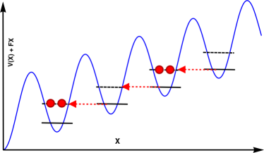
Figure 1: (Color online) Schematic representation of doublon-holon creation in a strongly tilted optical lattice triggered via resonant tunneling between single (solid line) and two-particle (dashed line) states at $F\approx U$.

II SECOND ORDER PROCESS IN THE STRONG TILTING REGIME

The starting point in our analysis is the single-band one-dimensional Bose-Hubbard Hamiltonian for $N$ bosonic atoms within $L$ lattice sites Kolovsky2003

$$\hat{H}=\sum_{l}Fl\hat{n}_{l}+\frac{U}{2}\hat{n}_{l}(\hat{n}_{l}-1)-J(\hat{a}_{l+1}^{\dagger}\hat{a}_{l}+{\rm h.c.})\,,$$ (1)

Here we set $\hbar=1$ and the lattice constant is also set to one. The operators $\hat{a}_{l}^{\dagger}$ and $\hat{a}_{l}$ are the bosonic creation and annihilation operators, and $\hat{n}_{l}$ is the number operator. We assume unit filling lattice, that is $s_{0}\equiv N/L=1$, for which the dimension of the Fock basis, $\{|n_{0}n_{1}\cdots n_{L-1}\rangle\}$, is $d_{\rm Fock}=(2L-1)!/[L!(L-1)!]$. We restrict our analysis to the regime of strong Stark field such that $F\sim U$, and $\{J,\,|U-F|\}\ll\{U,\,F\}$. As shown by Sachdev et al. Sachdev2002 , within this regime first order processes allow for the creation of dipole excitation consisting of a pair doublon-holon, that is, a state with two particles in a well and an unoccupied the nearest neighboring well as sketched in Fig. 1. The type of states with only one doublon-holon, i.e., a state with the form $|111\cdots 201\cdots 1\rangle$ will be the main focus in our analysis.

To successfully generate appropriate conditions for the propagation of dipoles, a first step has to be done: To prepare of an initial state $|\psi_{0}\rangle=|111\cdots 201\cdots 1\rangle$. To do so, a Mott insulator is prepared in an untilted optical lattice ($F=0$) which is expected to be sufficiently stable in the chosen parameter regime (see Greiner2002 ). At this stage a doubly occupied site plus an empty one can be created by means of single-site addressing techniques reported in Fukuhara2013 . Given the previous step, our initial scenario is completed after suddendly quenching the Stark field from $\hat{H}(F=0)\rightarrow\hat{H}(F\neq 0)$ such that $F>0$ is far apart from any possible single and/or many-particle tunneling resonances, that is, $\lambda\equiv F/U>1$. Thereby, the system is expected to be dynamically frozen since first-order tunneling processes are not allowed by construction. The creation of a doublon implies the simultaneous creation of an empty site, here, reffered to as holon owing to its quasiparticle nature Andraschko2015 . We have then a quasiparticle consisting of a hole and a doublon, both together forming a quantum dipole. From the point of view of spin-1/2 systems this procedure corresponds to the flipping of only one spin in a chain Fukuhara2013 . Within this context it will be shown later that dipole propagation relates to the superexchange interaction.

The set of states of the type $\{|111\cdots 201\cdots 1\rangle,\cdots\}$, i.e., those ones having a doubly occupied- and an empty site togheter, spans an excitation manifold accessible by local hopping processes from the Mott-insulating state $|1111111\cdots 1\rangle$. This manifold is characterized by the conservation of the quantum dipole number $\langle\sum\nolimits_{l}\hat{d}_{l}^{\dagger}\hat{d}_{l}\rangle_{t}$, where $\hat{d}_{l}^{\dagger}\propto\hat{a}^{\dagger}_{l-1}\hat{a}_{l}$ is the creation operator for dipoles. The dimension of this manifold, $d_{\rm dip}$, is very much smaller than the dimension, $d_{\rm Fock}$, of the Fock space corresponding of the full Bose-Hubbard Hamiltonian. In a previous work was shown that within this manifold subspace the Bose-Hubbard Hamiltonian can be mapped onto an antiferromagnetic spin-1/2 chain embedded in a transversal and longitudinal magnetic fields Sachdev2002 . This extraordinary simplification was experimentally confirmed by the group of Greiner et al. Simon2011 , thus establishing one of the first realization of a quantum simulation of one-dimensional quantum magnetism in optical lattices.

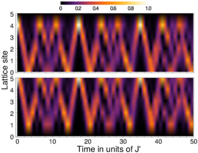
Figure 2: (Color online) Density profile showing the propagation in time of (top) the doublon and (bottom) the holon for $\lambda=3$ which are constructed by the filtering procedure describes in the main text. The initial state was $|111120\rangle$, for $L=6$. Note that both doublon and holon follow the same dynamical behavior along the lattice and are always one beside the other thus confirming their motion as that of a single unique quasiparticle, the doublon-holon or dipole excitation. The BH parameters are those mentioned in text and $J^{\prime}$ is defined in Eq. (6).

We investigate dynamical effects beyond the resonant regime depicted in Fig. 1. To do so, we evolve in time the initial state $|\psi_{0}\rangle=|111\cdots 120\rangle$ and compute the lattice site doublon and holon occupation numbers

$$\langle\hat{b}_{l}\rangle_{t} = \frac{1}{2}\langle\psi_{0}|\hat{U}^{\dagger}_{t}\,[\hat{n}_{l}(\hat{n}_{l}-1)]\,\hat{U}_{t}|\psi_{0}\rangle$$

$$\langle\hat{h}_{l}\rangle_{t} = \frac{1}{2}\langle\psi_{0}|\hat{U}^{\dagger}_{t}\,[(\hat{n}_{l}-1)(\hat{n}_{l}-2)]\,\hat{U}_{t}|\psi_{0}\rangle\,,$$ (2)

to track the dipole propagation along the lattice. The time evolution operator is defined by $\hat{U}_{t}=\exp(-i\hat{H}t)$. Note that the observables defined in Eq. (II) allows us to filter the individual dynamical evolution of the doublon and the holon. However, as shown in Fig 2, it is now clear that these two move together without splitting across the lattice . This means that in order to characterize the dipole wavefunction it is enough to track one of its components, i.e., either the doublon or the holon. From Fig. 2 we also recognize that the dipole wavefunction delocalizes in space in its in-lattice motion from one lattice edge to the opposite one. The dipole wavefunction then starts highly localized and undergoes a spreading processes in its first edge-to-edge transit. This delocalization takes place as a smooth transition between manifold states, that is, from $|111\cdots 120\rangle\rightarrow|111\cdots 1201\rangle$ which is not possible by means of a single hopping action. At the opposite edge the dipole wavefunction is partially relocalized and the structure of the state is $|201\cdots 111\rangle$. This clean and coherent dynamics occurs within the $\lambda$-range $\{2.5,\cdots,4\}$, where $x\equiv F/U$. For $\lambda\gg 1$ the dipole remains frozen, i.e., it does not propagate along the lattice. The other limit, the one for which $\lambda\rightarrow 1$ implies an interplay between first- and second-order tunneling processes, which is translated to the creation/annihilation of dipoles induced by resonant tunneling effects at $F\approx U$, and the edge-to-edge dipole propagation, respectively. From now onwards we fix $\lambda=3$ and the Bose-Hubbard parameters are taken from Ref. Meinert2013 , that is $J=0.0254\,{\rm kHz}$ and $U=1.019\,{\rm kHz}$.

After the first edge-to-edge transit owing to the presence of boundaries the wavefunction gets reflected and the dipole is driven backwards. However, the subsequent transit is not as before since the wavefunction present a bifurcation which relates to dynamical self-interference effects. The mechanism for this to occur is the fact that both doublon and holon when reflected at the boundary adquire dynamical phases which influence the backward transit (see Fig. 2). Yet, irrespective of the dynamical self-interference it can be noticed that the localization properties of the dipole wavefunction are recovered and, naturally, after a certain time the initial state $|\psi_{0}\rangle$ is reconstructred resembling a sort of echo dynamics Hahn1950 . This localization-delocalization process is periodic in time and its characeristic period $T$ depends on the system size $L$.

In order to characterize this underlying dynamics of the strongly tilted Bose-Hubbard model in the off-resonant regime, we construct an effective Hamiltonian accounting for the main mechanism for the dipole propagation along the lattice. This effective model will allow us to describe accurately the physical phenomenology involved in the motion of quantum dipoles in an optical lattice. The major difficulty appearing when analyzing large systems in the full Bose-Hubbard context is that the dimension of the associated Fock space increases exponentially with the number of lattice sites. Then a systematic analysis of the above mentioned effects becomes untractrable for $L\gg 1$. With the effective model this study gets easier.

III EFFECTIVE MODEL FOR DIPOLES

Since the Bose-Hubbard model (1) does not explicitly allow for the motion of particles beyond single hopping. We therefore construct an effective Hamiltonian accounting for two sucessive hopping processes required for the dipole to move, that is, the transition between manifold states. This action requires the participation of an auxiliary state, for example, the Mott-insulating state $|111111\cdots 1\rangle$. An efficient way to obtain the sort of model we look for is by means of the Schrieffer-Wolff transformation (SWT) Schrieffer1966 ; Chan2004 . The transformation consists in separating the Hamiltonian as $\hat{H}=\hat{H}_{0}+\hat{V}$, where $\hat{V}$ is a perturbation to the Hamiltonian $\hat{H}_{0}$ for which its eigenvalues and eigenvectors are known. Since $J\ll U$ the hopping part might be treated as the perturbation $\hat{V}$. We now have to find out an antiunitary operator $\hat{S}$ such that

$$\hat{H}^{\rm eff}=e^{\hat{S}}\hat{H}e^{-\hat{S}}\approx\hat{H}_{0}+\frac{1}{2}[\hat{S},\hat{V}]\,,$$ (3)

given the constrain $\hat{V}=-[\hat{S},\hat{H}_{0}]$. In general to find out $\hat{S}$ is not an easy task, but the use of the eigensystem solution of $\hat{H}_{0}$ allows us to write the matrix elements of $\hat{H}^{\rm eff}$ as

$$H^{\rm eff}_{ij}=\varepsilon_{i}\delta_{ij}+\frac{1}{2}\sum_{k\neq i,j}\left[\frac{1}{\varepsilon_{i}-\varepsilon_{k}}-\frac{1}{\varepsilon_{k}-\varepsilon_{j}}\right]V_{ik}V_{kj}\,,$$ (4)

where $V_{ij}=\langle i|\hat{V}|j\rangle$. Note that the coupling between the eigenstates $|i\rangle$ and $|j\rangle$ of $\hat{H}_{0}$ via $\hat{V}$ involves the sum over all auxiliary states $|k\rangle\neq\,\{|i\rangle,|j\rangle\}$ for the required transition to occur.

We illustrate the implementation of Eq. (4) using the minimal system that can support dipole propagation, the system $N/L=3/3$. There are only two auxiliary states for the dipole hopping to occur (see fig. 3). First, to go from $|120\rangle$ to $|201\rangle$ an auxiliary state is the dipole vacuum given by the Mott state $|111\rangle$. Second, that transition is also possible via a second auxiliary state involving a holon and a doublon separated by one lattice site, that is, $|210\rangle$. The operator accounting for both of virtual processes is the same and its form is $a^{\dagger}_{2}a_{1}a^{\dagger}_{2}a_{3}$. An additional reduction can be done on the final Hamiltonian $\hat{H}^{\rm eff}$ that will depend on the tilting term $\sim Fln_{l}$ of $\hat{H}_{0}$. We can get rid of it working in the interaction picture computed with respect to the term $\sum\nolimits_{l}Fl\hat{n}_{l}$. This can be proven by showing that the commutator $[\hat{H}^{\rm eff},\sum_{l}Fl\hat{n}_{l}]=0$. We finally arrive to a translationally invariant and time-independent effective Hamiltonian for the dipoles given by

$$\hat{H}^{\rm eff}=\sum_{l}\frac{U}{2}\hat{n}_{l}(\hat{n}_{l}-1)+J^{\prime}(\hat{a}^{\dagger}_{l+1}\hat{a}_{l}\hat{a}^{\dagger}_{l+1}\hat{a}_{l+2}+{\rm h.c.})\,,$$ (5)

where

$$J^{\prime}=2\frac{J^{2}}{U}\left(\frac{1}{\lambda}+\frac{1}{\lambda-1}\right).$$ (6)

Note that now it is easy to recognize the dipole hopping term with strength $J^{\prime}$ responsible for the dipole propagation along the lattice. In Fig. 4-(top) we present the density profile of the doublon given the initial state $|\psi_{0}\rangle=|111120\rangle$. It was computed using the effective Hamiltonian (5) with open boundary conditions. As it can be seen, the effective model captures the principal characteristics of the full model (1), namely, propagation and dynamical interference (see Fig. 4-(top)).

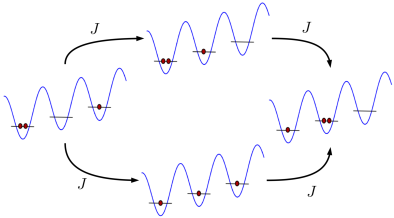
Figure 3: (Color online) Schematic representation of the second order processes driving the transition between dipole states via two successive single-particle hopping processes involving auxiliary states.

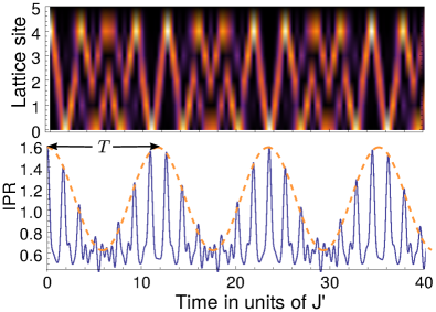
Figure 4: (Color online) (Top) Density plot showing the evolution in time of the dipole excitation (only doublon shown) which propagates along the lattice. This was computed using the effective Hamiltonian (5), with the initial state $|111120\rangle$ with open boundary conditions. (Bottom) IPR of the density plot as a function of time. The orange-dashed line represents the enveloping function that permits to recognize the periodical motion.

Yet, there are subtle differences. For instance, in the framework of the effective Hamiltonian the dipole wavefunction after the first interference passage has to bounce twice at the edges in order to gain the dynamical phase enough to, again, trigger the self-interference pattern. As a consequence, the second pattern is inverted with respect to the first one. In spite of this dephasing-induced effect, one can notice that the time required for the appearance of this second pattern is the same in both full and effective model.

Our dipole is a whole complex structure robust to the in-lattice propagation. This can be shown when mapping the bosonic hopping operators into dipole creation (annihilation) operators, as introduced in ref. Sachdev2002 ,

$$\hat{d}_{l}^{\dagger}=\frac{\hat{a}_{l+1}^{\dagger}\hat{a}_{l}}{\sqrt{s_{0}(s_{0}+1)}}\,,$$ (7)

with $s_{0}=1$ the average lattice filling. The number of dipoles per site is restricted to either zero or one, and dipoles in nearest neighboring sites are not allowed. These restrictions translate to

$$\hat{d}_{l}^{\dagger}\hat{d}_{l}\leq 1\qquad\text{and}\qquad\hat{d}_{l+1}^{\dagger}\hat{d}_{l+1}\hat{d}_{l}^{\dagger}\hat{d}_{l}=0\,.$$ (8)

The effective model (5) under these constrains reduces to

$$\hat{H}_{\rm dip}=\sum_{l}(U-F)\hat{d}_{l}^{\dagger}\hat{d}_{l}+2J^{\prime}(\hat{d}_{l+1}^{\dagger}\hat{d}_{l}+{\rm h.c.})\,,$$ (9)

which describes the dipole as a single quasiparticle moving along the lattice. The term $U-F$ accounts for the detunning between the single and two-particle levels that allow for the creation of a doublon sketched in Fig. 1. In our regime of interest this diagonal term can be neglected because of the dipole number conservation.

The dipole representation is useful for the study of the localization properties of the dipole wavefunction. This is done by defining the Inverse Participation Ratio (IPR)

$${\rm IPR}=\int_{\rm Lattice}|\rho(x,t)|^{2}{\rm d}x\,,$$ (10)

where $\rho(x,t)$ is the normalized dipole density probability distribution

$$\rho(x,t)=\sum_{l}\langle\hat{d}_{l}^{\dagger}\hat{d}_{l}\rangle_{t}\,\delta(x-l)\,,$$ (11)

and we have defined

$$\langle\hat{d}_{l}^{\dagger}\hat{d}_{l}\rangle_{t}=\langle\psi_{0}|e^{i\hat{H}_{\rm dip}t}\,\hat{d}_{l}^{\dagger}\hat{d}_{l}\,e^{-i\hat{H}_{\rm dip}t}|\psi_{0}\rangle.$$ (12)

In Fig. 4-(bottom) we plot the IPR correponding to the density profile of the system $L=6$. The IPR shows that indeed the dipole wavefunction delocalizes in every edge-to-edge transit where only two manifold states are relevant, then IPR${}_{\rm min}\approx 0.5$ (see Fig. 4-(bottom)). The self-interference regions are characterized by the spreading of the wavefunction, follwed by relocalization of this after certain time. This periodic behavior is highlighted by the enveloping function (orange-dashed line) from which the period $T$ can be extracted.

The propagation of dipoles can be interpreted even in a more fashionable representation consisting of spins. Following Ref. Sachdev2002 we use the pseudo spins transformation defined by $\hat{\sigma}_{l}^{+}=2\hat{d}_{l}$, $\hat{\sigma}_{l}^{-}=2\hat{d}_{l}^{\dagger}$ and $\hat{\sigma}_{l}^{z}=1-2\hat{d}_{l}^{\dagger}\hat{d}_{l}$, to rewrite Eq. (9) in the spin representation resulting in the Heisenberg XXZ model

$$\hat{H}_{\rm spin} = \frac{W}{4}\sum_{l}\hat{\sigma}_{l}^{z}\hat{\sigma}_{l+1}^{z}+J^{\prime}\sum_{l}(\hat{\sigma}_{l}^{x}\hat{\sigma}_{l+1}^{x}+\hat{\sigma}_{l}^{y}\hat{\sigma}_{l+1}^{y})$$ (13)

$$- \frac{1}{2}(W+U-F)\sum_{l}\hat{\sigma}_{l}^{z}\,,$$

where $\hat{\sigma}_{l}^{x,y,z}$ are Pauli matrices, and the parameter $W$ is an extra energy term of order $U$. Here, it is clearly seen that the dipole propagation mechanism is nothing but the superexchange interaction which locally flips two nearest neighboring spins in a chain. Then, it allows for the motion of only one flipped spin or spin impurity Fukuhara2013 in a medium consisting of spins with opposite polarization. Likewise, the creation of a dipole translates to flipping one single spin in a chain with the Mott-insulating phase, $|111111\cdots 1\rangle$, represented by the state $|\downarrow\downarrow\downarrow\cdots\downarrow\rangle$. The strength of the effective magnetic field is $h=(W+U-F)/2$, and the anisotropy parameter is given by $\Delta=W/4J_{\rm exc}$, with $J_{\rm exc}=2J^{\prime}$ the superexchange coupling strength. Given the order of magnitude of the Bose-Hubbard parameters used throughout this paper we have $\Delta\gg 1$ meaning that the dynamics of our system is deep inside the Néel (antiferromagnetic) phase of the Heisenberg XXZ model (see details in Ref. Mikeska2004 ).

Unfortunately, the one dimensional XXZ model (13) is analitically untractable, that is, to obtain its eingenstates one has to implement numerical diagonalization, for instance, using the Lanczos algorithm ParraMurilloCPC . Nevertheless, in our analysis we found that the effective dimensions of the new Hamiltonians (9) and (13) are much smaller than the dimension of the full Hamiltonian. In the case of the spin Hamiltonian the dimension is $d_{\rm spin}=2^{L}\ll d_{\rm Fock}$, and for the case of the dipole basis $\{|000\cdots 01_{i}0\cdots 0\rangle\}$ the number of accessible states $d_{\rm dip}=L\lll d_{\rm Fock}$. All this implies a fantastic reduction of computational resources for the analysis of suficiently large lattices. We then devote the rest of this paper to study and characterize the self-interference effect and the diffusive behavior of our system usin these effective models.

IV QUANTUM DIFFUSION AND EMERGENCE OF MATTER QUANTUM CARPETS

IV.1 Short-time dynamics

The localization properties previously described can be studied in a more accurate way for the short-time dynamics using the effective dipole Hamiltonian (8). Here, we show that the dipole wavefunction in the first edge-to-edge transit undergoes a ballistic delocalization, followed by a normally diffusive evolution right after its first reflection at the lattice borders. To do so, we assume open boundary conditions and invoke the fact that the Hamiltonian $\hat{H}_{\rm dip}$ describing a quasiparticle confined in an untilted periodic potential is diagonal in the quasimomentum space. This latter is straighforwardly proven by expanding the bosonic lattice operators in their respective fourier series as $\hat{d}_{l}=L^{-1/2}\sum\nolimits_{k}e^{ikl}\hat{d}_{k}$, $\hat{H}_{\rm dip}$ transforms the effective Hamiltonian into

$$\hat{H}_{\rm dip}(k)=\sum_{k}\varepsilon(k)\hat{d}_{k}^{\dagger}\hat{d}_{k}\,,$$ (14)

with $\varepsilon(k)=F-U+4J^{\prime}\cos(k)$ being the quasiparticle dispersion relation valid for suffiently large lattice. This formula brings advantages at obtaining an analitycal expression for the dipole site occupation $\langle\hat{d}_{l}^{\dagger}\hat{d}_{l}\rangle_{t}$ Hofmann2012 which results in

$$\langle\hat{d}_{l}^{\dagger}\hat{d}_{l}\rangle_{t}=\mathcal{J}_{l-l_{0}}^{2}(4J^{\prime}t)\,.$$ (15)

$\mathcal{J}_{l-l_{0}}(t)$ is the Bessel function of the first kind and $l_{0}$ is the starting location of the dipole. The comparison of both numerical and theoretical density profiles is shown in Fig. 5, where not relevant differences are observed before the reflection at the edges. The ballistic wavefunction spreading in time is shown by computing the variance of the occupation dipole distribution (10) $\sigma^{2}=\langle\hat{x}^{2}\rangle-\langle\hat{x}\rangle^{2}$ for which an analytic expression is obtained using Eq. (15). The calculation follows as

$$\sigma^{2} = \sum_{l}l^{2}\mathcal{J}_{l-l_{0}}^{2}(4J^{\prime}t)\left(1-\mathcal{J}_{l-l_{0}}^{2}(4J^{\prime}t)\right)$$ (16)

$$\approx \sum_{l\neq l_{0}}l^{2}\mathcal{J}_{l-l_{0}}^{2}(4J^{\prime}t)\,,$$

where we have used the fact that the Bessel function of the first kind, of the order $|l-l_{0}|>0$, are negligible if $4J^{\prime}t\ll 1$. Now by expanding the Bessel function $\mathcal{J}_{l-l_{0}}(4J^{\prime}t)$ up to the first order we can write

$$\mathcal{J}_{l-l_{0}}^{2}(4J^{\prime}t) \approx \frac{1}{(l-l_{0})!^{2}}(2J^{\prime}t)^{2(l-l_{0})}$$ (17)

$$+ \frac{1}{(l-l_{0}+1)!^{2}}(2J^{\prime}t)^{2(l-l_{0}+2)}$$

$$- \frac{2}{(l-l_{0})!(l-l_{0}+1)!}(2J^{\prime}t)^{2(l-l_{0}+1)}\,,\,\,\,\,\,\,\,$$

which helps us to evaluate Eq (16) to obtain the variance as a function of time

$$\sigma^{2}\approx\sum_{l\neq l_{0}}l^{2}\mathcal{J}_{l-l_{0}}^{2}(4J^{\prime}t)=8(J^{\prime}t)^{2}\propto{\rm IPR}^{-1}\,.$$ (18)

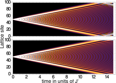
Figure 5: (Color online) Short-time evolution of the occupation site distribution for $L=100$ with the dipole initially placed in the middle of the lattice. (Top) Using the effective Hamiltonian (9) with open boundary conditions, and (bottom) Using the analytic expression (15).

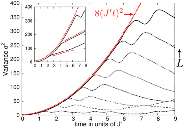
Figure 6: (Color online) Variance $\sigma^{2}$ of the dipole wavefunction for $L=\{12,18,\cdots,54\}$ from down to up. The red-dasehd line represent is the theoretical prediction in Eq. (18). The inset shows the dependence of $\sigma^{2}$ on the location $l_{0}$ of the initial dipole $l_{0}=27$ at the center of the lattice and $l_{0}=\{8,14\}$ (The two lowest ones) for a fixed lattice sites number $L=54$. The straight red-dashed lines correspond to the normal diffusion tendency of the wavefunction spreading right after its contact with the boundaries.

The dipole wavefunction then diffuses anomalously since $\sigma^{2}\propto t^{2}$. The spreading of the wavefuction is then faster than the one for Brownian particles or a particle in a classical random walk. This behavior is exhibited in Fig. (6) where we have computed the variance of the dipole wavefunction as a function of time for increasing the system size $L$ where, as shown above, before arriving to the first edge the dipole wavefunction undergoes the ballistic spreading.

Boundary effects on the dyamics are usually much complicated to be analitically computed. We numerically study the border effect by initializing the wavefunction at different location in the lattice, that is, as a function of $l_{0}$. We set open boundary conditions. The results are plotted in the inset of Fig. (6) for a lattice with $L=54$. The dynamical variance for the first edge-to-edge transit preserves the power-law dependence obtained in Eq. (18), while for backwards transit right after the reflection at the boundary the diffusive spreading slows down. The plot is done for the initial locations $l_{0}=27$, i.e., right in the center of the lattice, and two cases closer to the border for which $l_{0}=\{8,14\}$. The dipole wavefunction initialized close to the border undergoes a backwards diffusive transit after reflecting at the borders for which its variance now changes linearly in time, $\sigma^{2}\propto t$ (see red-dashed straight lines in the inset). It is then expected that for a dipole set initially at one of the border the spreading of the wavefunction becomes nearly normally diffusive in its first edge-to-edge transit.

IV.2 Long-time dynamics

The self-interference pattern in Fig. (2) is a finite size effect and appears no matter which of the two classes of boundary conditions we imposed, i.e., the open or the periodic ones. However, relocalization of the dipole wavefunction is seen to be only possible for open boundary conditions which admit recurrences for finite lattice size. We have also seen that the delocalization-localization process is periodic (see Fig. (2-4)) in time, whose period $T$ can be extracted from the IPR (10) and analyzed in terms of the system size.

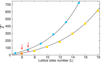
Figure 7: (Color online) Interference time as a function of system size $L$, with $L=\{5,6,\cdots,18\}$, for odd $L$ ($\bullet$) and even ($\blacksquare$). The lines represent the best fits and the red asterisk are the interference time computed with the full model for lattices with $L=6$ and $L=7$ sites. These calculations were done for open boundary conditions.

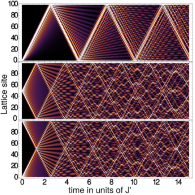
Figure 8: (Color online) Density profile of the dipole wavefunction propagation along the lattice for a chain with $L=100$ sites. The initial condition corresponds to (Top) a dipole placed in one corner $|0100\cdots 000\rangle$, (Middle) a dipole in the middle of the lattice $|00\cdots 010\cdots 00\rangle$, both cases with open boundary conditions, and (Bottom) periodic boundary conditions and the same initial state as in the top panel.

Fig. 7 shows the dependence of $T$ on the increasing lattice site number $L$ and on its parity. For $L$ odd the self-interference pattern is preserved longer than for the case of $L$ even. In both cases $T$ grows exponentially with the system size. This result, valid only for open boundary conditions, cannot be extrapolated to a thermodynamic limit $L\rightarrow\infty$ because the self-interference occurs as a consequence of the reflecting borders. For periodic boundary conditions, the interference appears because of the dynamical wrapping of the wavefunction on the surface of a cylinder of diameter $L/\pi$. Thus, the interference pattern is a consequence of the encounter of counterpropagating principal and secondary waves (see Fig. 8), an effect that has not recurrences. Therefore $T\rightarrow\infty$ presenting an unique and everlasting interference pattern. The complex dynamical pattern observed in Fig. 8 is nothing but the so-called quantum carpet  Berry2001 .

Self-interference might be understood by inspecting the delocalization process of the dipole wavefunction when travelling along the lattice. The transit from one site to the nearest neighbor induces, due to local reflections, small secondary waves-like components which also travel in the same direction of the principal wave when the dipole is initialized at one of the edges. This is also clear after inspecting Eq. (15) within the time regime for $0<t\ll 1/4J^{\prime}$. Yet, those secondary waves are retarded in time arriving late at the edge interfering with the already reflected principal wave (see Fig. 8-(middle)). This generates a final and sufficiently complex interference pattern, the quantum carpet. In the case of a dipole initialized, for example, in the middle of the lattice, two principal waves appears owing to the translational invariance of our system. Thus, the generated secondary waves travel both directions then triggering intereference effect at both edges of the lattice simultaneously (see Fig. 8-(middle)). The same occurs for an initial dipole state at one of the edges when imposing with periodic boundary conditions for which also intereference effects appear in the middle of the lattice (see Fig. 8-(bottom)).

V SUMMARY AND CONCLUSIONS

We have studied a single-band tilted Bose-Hubbard Hamiltonian in one dimension showing that far from single particle and two-particle level resonances there is still very interesting dynamical effects. The phenomenology induced by the propagation of a quasiparticle made of a doublon and a holon, that we called dipole excitation or exciton, shows the appearance of finite size dynamical self-interference pattern. This effect is known as a quantum carpet and can be understood as the interference of the principal and secondary wave components of the time-evolved dipole wavefunction. We also show that for large but finite system sizes $L$ the emergent interference pattern lasts very long, and its caracteristic time $T$ grows exponentially with $L$. We derive an analytic expression for the dipole site occupation for short times that allow us to determine the diffusive properties of our system. Here, it has been shown that the spreading of the wavefunction is superdiffusive, a ballistic behavior similar to the one presented in Refs. Andraschko2015 ; Hofmann2012 , yet for a doublon-holon excitation in a unit-filled tilted optical lattice, and not in an empty one. Furthermore, we study the effect of the borders in the dynamics showing that right after the border, for a dipole initialized close to the edges, the diffusive spreading is slowed down becoming normal, that is, the wavefunction variance grows linearly with the time.

The results presented in this paper can be straightforwardly implemented in experiments using ultracold atoms trapped in optical lattices as, for instance, an extension of the works done by F. Meinert et al Meinert2013 ; Meinert2014 and Simon et al. Simon2011 . We suggest to explore the regime of strong tilts, Stark fields, far from the many-particle first order of resonances where our results take place.

VI Acknowledgments

The authors acknownledge the finantial support of the University del Valle (project CI 7996). C. A. Parra-Murillo greatfully acknowledges the financial support of COLCIENCIAS (grant 656). We warmly thank to Dr. A. Argüelles for the lively discussion and critical reading of our manuscript.

References

- (1) H. A. Gersch and G. C. Knollman, Phys. Rev. 129, 959 (1963).
- (2) M. P. A. Fisher, P. B. Weichman, G. Grinstein, and D. S. Fisher, Phys. Rev. B 40, 546 (1989).
- (3) D. Jaksch, C. Bruder, J. I. Cirac, C. W. Gardiner, and P. Zoller, Phys. Rev. Lett. 81, 3108 (1998).
- (4) M. Lewenstein, A. Sanpera, V. Ahufinger, B. Damski, A. Sen De, and U. Sen, Adv. Phys. 56, 243 (2007).
- (5) I. Bloch, J. Dalibard, and W. Zwerger, Rev. Mod. Phys. 80, 885 (2008).
- (6) M. Greiner, O. Mandel, T. Esslinger, Th. W. Hänsch, and I. Bloch, Nature 415, 39-44 (2002).
- (7) M. Ben Dahan, E. Peik, J. Reichel, Y. Castin, and C. Salomon. Phys. Rev. Lett., 76, 4508 (1996).
- (8) M. Glück, A. R. Kolovsky, and H. J. Korsch, Phys. Rep., 366 103 (2002).
- (9) J. Simon, W. S. Bakr, R. Ma, M. E. Tai, P. M. Preiss, and M. Greiner, Nature 472, 307 (2011).
- (10) F. Meinert, M. J. Mark, E. Kirilov, K. Lauber, P. Weinmann, A. J. Daley, and H.-C. Nägerl, Phys. Rev. Lett. 111, 053003 (2013).
- (11) F. Meinert, M. J. Mark, E. Kirilov, K. Lauber, P. Weinmann, M. Gröbner, and A. J. Daley, H.-C. Nägerl, Science 344, 1259 (2014).
- (12) S. Sachdev, K. Sengupta, and S. M. Girvin, Phys. Rev. B 66, 075128 (2002).
- (13) A. R. Kolovsky, Phys. Rev. A 70, 015604 (2004).
- (14) C. Sias, A. Zenesini, H. Lignier, S. Wimberger, D. Ciampini, O. Morsch, and E. Arimondo, Phys. Rev. Lett. 98, 120403 (2007); A. Zenesini, H. Lignier, G. Tayebirad, J. Radogostowicz, D. Ciampini, R. Mannella, S. Wimberger, O. Morsch, and E. Arimondo, Phys. Rev. Lett. 103, 090403 (2009).
- (15) P. Plötz, P. Schlagheck, and S. Wimberger, Eur. Phys. J. D 63, 47 (2011); P. Plötz, J. Madroñero, and S. Wimberger, J. Phys. B. 43, 08001(FTC) (2010).
- (16) C. A. Parra-Murillo, J. Madroñero, and S. Wimberger, Phys. Rev. A 88, 032119 (2013). C. A. Parra-Murillo, J. Madroñero, and S. Wimberger, Phys. Rev. A 89 (5), 053610 (2014).
- (17) L. Amico, R. Fazio, A. Osterloh, and Vlatko Vedral, Rev. Mod. Phys. 80, 517 (2008).
- (18) M. Endres, M. Cheneau, T. Fukuhara, C. Weitenberg, P. Schauß, C. Gross, L. Mazza, M. C. Banuls, L.Pollet, I. Bloch, and S. Kuhr, Appl. Phys. B, 113, (1) 23 (2013).
- (19) D. Greif, M. F. Parsons, A. Mazurenko, C. S. Chiu, S. Blatt, F. Huber, G. Ji, and M. Greiner, arXiv:1511.06366 [cond-mat.quant-gas].
- (20) T. Fukuhara, A. Kantian, M. Endres, M. Cheneau, P. Schauß, S. Hild, D. Bellem, U. Schollwöck, T. Giamarchi, C. Gross, I. Bloch, and S. Kuhr, Nat. Phys. 9, 235 (2013); M. Endres, M. Cheneau, T. Fukuhara, C. Weitenberg, P. Schauß, C. Gross, L. Mazza, M. C. Bañuls, L. Pollet, I. Bloch, and S. Kuhr, science 334, 200 (2011).
- (21) M. Aidelsburger, M. Atala, S. Nascimbène, S. Trotzky, Y.-A. Chen, and I. Bloch, Phys. Rev. Lett. 107, 255301 (2011).
- (22) K. Kim, M.-S. Chang, S. Korenblit, R. Islam, E. E. Edwards, J. K. Freericks, G.-D. Lin, L.-M. Duan, and C. Monroe, Nature, 465, 590 (2010).
- (23) M. G. Bason, M. Viteau, N. Malossi, P. Huillery, E. Arimondo, D. Ciampini, R. Fazio, V. Giovannetti, R. Mannella, and O. Morsch, Nature Physics 8, 147Ð152 (2012); L. Giannelli and E. Arimondo, Phys. Rev. A 89, 033419 (2014).
- (24) Y.-A. Chen, S. D. Huber, S. Trotzky, I. Bloch, and E. Altman, Nature Physics 7, 61Ð67 (2011).
- (25) A. Polkovnikov, Phys. Rev. B 72, 161201 (2005).
- (26) M. Wilkinson, J. Phys. A: Math. Gen. 21, 4021 (1988).
- (27) F. Andraschko and J. Sirker, Phys. Rev. B 91, 235132 (2015).
- (28) F. Hofmann and M. Potthoff, Phys. Rev. B 85, 205127 (2012).
- (29) D. Witthaut, F. Trimborn, H. Hennig, G. Kordas, T. Geisel, and S. Wimberger, Physical Review A 83 (6), 063608 (2011).
- (30) E. Hahn, Phys. Rev. 80, p.580 (1950).
- (31) A. R. Kolovsky and A. Buchleitner, Phys. Rev. E 68 056213 (2003).
- (32) J. Schrieffer and P. Wolff, Phys. Rev. 149, 491 (1966).
- (33) R. Chan and M. Gulácsi, Philosophical Magazine 84, 1265 (2004).
- (34) I. B. Spielman, Nature 472, 301 (2011).
- (35) H.-J. Mikeska and A. K. Kolezhuk, on Quantum Magnetism, Lecture Notes in Physics, vol 645, edited by U. Schollwöck, J. Richter, D. J. J. Farnell, and R. F. Bishop (Springer Verlag, Berlin, Heidelberg, 2004).
- (36) C. A. Parra-Murillo, J Madroñero, and S. Wimberger, Comp. Phys. Comm. 186, 19 (2015).
- (37) L. Vidmar, S. Langer, I. P. McCulloch, U. Schneider, U. Schollwöck, and F. Heidrich-Meisner, Phys. Rev. B 88, 235117 (2013).
- (38) S. Langer, F. Heidrich-Meisner, J. Gemmer, I. P. McCulloch, and U. Schollwöck, Phys. Rev. B 79, 214409 (2009).
- (39) Y. Sagi, M. Brook, I. Almog, and N. Davidson, Phys. Rev. Lett. 108, 093002 (2012).
- (40) M. V. Berry, I. Marzoli, and W. Schleich, Physics World (2001); A. E. Kaplan, I. Marzoli, W. E. Lamb, Jr., and W. P. Schleich, Phys. Rev. Ax 61, 032101 (2000).