Scalar field as an intrinsic time measure in coupled dynamical matter-geometry systems.
I. Neutral gravitational collapse

Abstract

There does not exist a notion of time which could be transferred straightforwardly from classical to quantum gravity. For this reason, a method of time quantification which would be appropriate for gravity quantization is being sought. One of the existing proposals is using the evolving matter as an intrinsic ‘clock’ while investigating the dynamics of gravitational systems. The objective of our research was to check whether scalar fields can serve as time variables during a dynamical evolution of a coupled multi-component matter-geometry system. We concentrated on a neutral case, which means that the elaborated system was not charged electrically nor magnetically. For this purpose, we investigated a gravitational collapse of a self-interacting complex and real scalar fields in the Brans-Dicke theory using the 2+2 spacetime foliation. We focused mainly on the region of high curvature appearing nearby the emerging singularity, which is essential from the perspective of quantum gravity. We investigated several formulations of the theory for various values of the Brans-Dicke coupling constant and the coupling between the Brans-Dicke field and the matter sector of the theory. The obtained results indicated that the evolving scalar fields can be treated as time variables in close proximity of the singularity due to the following reasons. The constancy hypersurfaces of the Brans-Dicke field are spacelike in the vicinity of the singularity apart from the case, in which the equation of motion of the field reduces to the wave equation due to a specific choice of free evolution parameters. The hypersurfaces of constant complex and real scalar fields are spacelike in the regions nearby the singularities formed during the examined process. The values of the field functions change monotonically in the areas, in which the constancy hypersurfaces are spacelike.

1 Introduction

The problem of time quantification is vital mainly in canonical approaches to quantum gravity, because in gravitational systems there does not exist a notion of time which could be straightforwardly transferred between the classical and quantum levels. The issue of measuring time is primarily significant in investigations of the dynamics of quantized gravitational systems. Moreover, seeking alternative descriptions of a gravitational system temporal evolution may become useful also in classical gravity, as they can potentially facilitate examining dynamics of complicated coupled matter-geometry systems.

The non-standard approach to measuring time during a process proceeding due to gravitational interaction is using the evolving matter itself in this regard DeWitt1967 . Also geometry could be used as a ‘clock’ when a dynamical evolution of matter is studied. In general, the dynamical behavior of a matter-geometry system can be followed with respect to one of its internal degrees of freedom, which serves as a reference for the remaining degrees of freedom and is interpreted as a dynamical observer. In order to obtain a successful description of the passage of time, two conditions have to be fulfilled during the investigated part of an evolution. First, the selected spacetime slices, parametrized by a time variable, ought to be spacelike. Second, the chosen time parametrization should remain monotonic during the course of the evolution of interest.

The idea of quantifying time described above has been widely employed in diversified analyses related to non-perturbative quantum gravity and quantum cosmology, which involve investigating a time evolution of a matter-geometry system without fixed geometry of a background spacetime Rovelli1991 . The constancy hypersurfaces of a scalar field were the spacelike slices parametrized by a time variable used in the construction of a Hamiltonian, which governed gauge transformations between these slices and thus described a quantum evolution of a gravitational field RovelliSmolin1994 . A scalar field was also treated as a time variable for the relational Dirac observables, whose dynamics was traced with respect to it DomagalaGieselKaminskiLewandowski2010 ; LewandowskiDomagalaDziendzikowski2012 . The inflation epoch of the Universe was examined in the regime of loop quantum gravity using a scalar field with an arbitrary potential with the gauge for the Hamiltonian constraints, which ensured that the constancy hypersurfaces of the scalar field were spacelike AlexanderMaleckiSmolin2004 . A similar approach involving a massless scalar field was used in loop quantum cosmology AshtekarPawlowskiSingh2006PRL ; AshtekarPawlowskiSingh2006PRD . The tunneling decay rate DabrowskiLarsen1995 of a simple harmonic universe GrahamHornKachruRajendranTorroba2014 was calculated with the use of a homogeneous, massless, minimally coupled scalar field additionally introduced to the model and having a negligible contribution to the total energy density of the system MithaniVilenkin2012 ; MithaniVilenkin2015 . A scalar field was treated as a common variable for internal time and a Hamiltonian evolution parameter during constructing a specific version of the Wheeler-DeWitt equation and its quantum timelike counterpart Perlov2015 . Apart from the scalar field, dust and radiative fluid were also used to provide a matter degree of freedom, which allowed tracing the temporal evolution of a gravitational system BrownKuchar1995 .

The non-minimally coupled to geometry Brans-Dicke scalar field, which is a part of the theoretical model considered in the present paper, was also analyzed in the context of time measurements in quantum cosmology ZhangArtymowskiMa2013-084024 . Since the field is a monotonic function of cosmological time, it was assumed to be a good candidate for an internal time variable. The cosmological Brans-Dicke model was quantized within the framework of loop quantum cosmology and the effective Hamiltonian was obtained under the assumptions of isotropy and spatial flatness. Unitarity of the evolution in the Brans-Dicke quantum cosmological model with a time variable in the form of an isotropic and homogeneous matter fluid was elaborated in AlmeidaBatistaFabrisMoniz2015 .

The Brans-Dicke theories are straightforward extensions of general relativity towards the scalar-tensor theories of gravity BransDicke1961-925 . The gravitational interaction is described within them by both a scalar field and the usual metric tensor of the Einstein theory. The effective gravitational coupling changes within the spacetime and asymptotically attains the value of the gravitational constant $G$. The strength of the coupling is determined by a scalar field which asymptotically tends towards the value of $G^{-1}$. The theory possesses the so-called Brans-Dicke coupling, $\omega$, which is a dimensionless constant. For its small values, the scalar constituent of the gravitational interaction predominates the tensor component, while for its large values the contribution of the tensorial part is more important. In the limit of $\omega\to\infty$ the Brans-Dicke theory becomes the Einstein theory Faraoni1999-084021 ; Will2014-4 . Several discussions on the problem whether this statement is correct in general or whether the conclusion depends on the value of the trace of the stress-energy tensor of the theory, the symmetry, staticity, stationarity or asymptotic flatness of the solutions, can be found, e.g., in RomeroBarros1993-243 ; Chauvineau2003-2617 ; ChauvineauSpallicciFournier2005-S457 ; Chauvineau2007-297 .

The Brans-Dicke theories have been tested against the experimental data. The most convincing analyses were done within the Solar System, as the considered theories are so close to the Einstein theory that they straightforwardly agree with all cosmological and astrophysical observations, at least for adequately big values of $\omega$ Will2014-4 . The frequency shift of the low energy photons due to the spacetime curvature experienced on their road to and from the Cassini spacecraft as they passed nearby the Sun confirmed the appropriateness of selected observational predictions of the Brans-Dicke theoretical construction BertottiIessTortora2003-374 .

The experimental restrictions on the value of the Brans-Dicke coupling can be posed on the basis of a series of astronomical observations and tests. The above-mentioned Cassini-Huygens experiment gave a lower bound on $\omega$ equal to $40000$ BertottiIessTortora2003-374 ; DeFeliceManganoSerpicoTrodden2006-103005 ; Will2014-4 . The supernovae Ia data provided the value of $-1.477$ within the Brans-Dicke cosmology with a pressureless fluid FabricGoncalvesRibeiro2006-49 and $-1.9$ in the dimensionally reduced theory Qiang2009-210 . When combined with the Hubble parameter versus the redshift relation measurements, information based on the Alcock-Paczyński test and the baryon acoustic oscillations observational data, the value of $\omega$ was estimated as $-0.8606$, $-1.1103$ and $-2.3837$ for several dynamical setups of the Brans-Dicke cosmology in the vicinity of the de Sitter state HrycynaSzydlowskiKamionka2014-124040 . The cosmic microwave background radiation temperature measurements performed by Planck allowed constraining the value of $\omega$ to be greater than $692$ Avilez2014-011101 . Their combination with the polarization data obtained by WMAP and the baryon acoustic oscillations distance ratio data from the Sloan Digital Sky Survey and the Six-degree-Field Galaxy Survey excluded the range from $-407.0$ to $175.87$ and preferred the values exceeding $181.65$ LiWuChen2013-084053 . According to the structure formation imprint in the cosmic background radiation, the lower limit of $\omega$ was equal to $120$ AcquavivaEtAl2005-104025 . As can be inferred from the above collection of diverse numerical data, the experiment-based values of the Brans-Dicke coupling are strongly model-dependent, since various assumptions about the symmetry and matter content of the analyzed spacetime were made in the outlined analyses. Moreover, the value of $\omega$ may change as the Universe evolves. The time scale of the dynamical process studied in the current paper, i.e., the gravitational collapse, is negligible in comparison to the cosmological time scales. For this reason, a set of constant values of the Brans-Dicke parameter was considered during the performed investigations.

During the cosmological evolution, the scalar contribution to gravity practically vanishes within most scalar-tensor formulations of gravity DamourNordtvedt1993-2219 ; DamourNordtvedt1993-3436 ; DamourPiazzaVeneziano2002-046007 . Hence, although $\omega$ is most probably large at present and for this reason the Brans-Dicke theory is currently experimentally indistinguishable from the Einstein theory, the value of the coupling could have been smaller in the past. For this reason, the class of the Brans-Dicke theories is widely studied in the context of the early stages of the evolution of the Universe. Unlike general relativity, it provides a satisfactory mechanism of the transition between the rapid inflationary stage of the Universe evolution and its later cosmological phase, which is called the extended inflation LaSteinhardt1989-376 ; MathiazhaganJohri1998-29 .

The corrections introduced by the Brans-Dicke theory to the current values of cosmological parameters such as the Hubble parameter, gravitational constant, or the usual fractions of energy density within the Friedman-Lemaître-Robertson-Walker cosmology, are negligible ArikCalik2005-013 ; ArikCalikSheftel2008-225 . The dimensionally reduced Brans-Dicke theory gave rise to models of an accelerated expansion of a matter-dominated universe which are consistent with current observations and with a decelerating radiation-dominated epoch SenSen2001-124006 ; QuiangMaHanYu2005-061501 ; deLeon2010-095002 ; deLeon2010-030 . The late-time acceleration of the Universe expansion was also examined within the Brans-Dicke theory under the assumption of the spatial flatness of the Universe Bisabr2012-427 ; Bisabr2012-127503 and in the presence of a fermionic field and a matter constituent described by the barotropic equation of state SamojedenDevecchiKremer2010-027301 ; Liu2010-063523 . Cosmological implications of holographic dark energy NojiriOdintsov2006-1285 ; CapozzielloNojiriOdintsov2006-597 ; Setare2007-99 ; Setare2010-1 and the stability of agegraphic dark energy FarajollahiSadeghiPouraliSalehi2012-79 were analyzed in the considered theory, while the new holographic dark energy model was studied in the framework of chameleon Brans-Dicke cosmology ChattopadhyayPasquaKhurshudyan2014-3080 . The isotropic and homogeneous Brans-Dicke model with a quartic scalar field potential and barotropic matter explained the accelerated expansion of the Universe without any assumptions about the properties of dark matter and dark energy HrycynaSzydlowski2013-016 . Constraints on a flat isotropic and homogeneous Brans-Dicke cosmological model with matter in the form of a perfect fluid with a constant equation of state parameter were presented in PaliathanasisTsamparlisBasilakosBarrow2015-arxiv . The evolution of the radius and mass of black holes in an expanding isotropic universe was discussed using the Einstein-Straus model EinsteinStraus1945-120 in the Brans-Dicke theory SakaiBarrow2001-4717 . The employed so-called ‘Swiss cheese’ model described the Friedman-Lemaître-Robertson-Walker universe, in which spherical regions were replaced by Schwarzschild spacetimes.

For finite values of $\omega$, the Brans-Dicke theory describes, under certain conditions, a bouncing cosmology Novello2008-127 , as the scale factor does not vanish during the backward temporal evolution of the Universe FabrisFurtadoPeterPintoNeto2003-124003 ; TretyakovaShatskiyNovikovAlexeyev2012-124059 ; TretyakovaLatoshAlexeyev2015-185002 . Its value decreases to a minimum and then increases, which allows avoiding the presence of the initial singularity of the classical general relativistic cosmology. The spatially flat and isotropic cosmological model of the Brans-Dicke theory with $\omega\neq-1.5$ was quantized within the loop quantum cosmology approach ZhangArtymowskiMa2013-084024 ; ArtymowskiMaZhang2013-104010 . In such a setup of the effective loop quantum Brans-Dicke cosmology, the classical initial singularity is replaced by a quantum bounce.

The researches on using matter as a time variable described at the beginning of this section did not address the issue of the relevance of such an idea. The behavior of matter during the investigated part of an evolution and within the studied spacetime region was assumed to be appropriate from the perspective of using it as a ‘physical clock’. The selected spacetime slices were presumed to remain spacelike and the chosen time parametrization was presumed to be monotonic during the whole process. The arguments supporting these assumptions are limited to certain cases (e.g., the homogeneity of a scalar field during the inflation initial phase, which results in a spacelike character of the field constancy hypersurfaces AlexanderMaleckiSmolin2004 ). Hence, there exists a need for research on dynamical processes, which will justify or contradict the above-mentioned assumptions. An introductory attempt in respect of validating these premises was made using the simplest matter-geometry model, which involved a gravitationally self-interacting scalar field minimally coupled to gravity NakoniecznaLewandowski2015-064031 . It turned out that the sole scalar field evolving in the spacetime under the influence of gravitational self-interaction possesses properties, which predestine it for being a time measurer, especially in the area of high curvature nearby the singularity. However, since the examined field was the only matter component in the spacetime, the conducted studies are not relevant to justify using the scalar field as a ‘clock’ in more general cases, which involve more matter components coupled to each other and to geometry.

In the present paper the dynamical collapse of an uncharged complex scalar field within the Brans-Dicke theory was considered in the context of time quantification using dynamical scalar fields. The assumed model also enabled us to analyze the results of a gravitational evolution of a self-interacting real scalar field in the Brans-Dicke theory. The structures of dynamical spacetimes which form during the investigated process were described. The main objective of the research was to examine whether the scalar field and the Brans-Dicke field can be used as time variables in the vicinity of the emerging singularity, which is a region of high curvature, as such regions are of crucial importance for the quantum gravity applications. The conducted studies focused on the role of couplings among the components of the considered model in order to assess their significance when scalar fields are to be used as time measurers in the dynamical system. The gravitational collapse itself is extensively studied in quantum gravity Torres2014-169 ; Torres2015-245 ; Vaz2015-558 ; GambiniPullin2015-19 . From the viewpoint of the field behavior in a spacetime, its course is more complicated than the usually studied spatially homogeneous cosmological evolution.

The Brans-Dicke theory was chosen for our studies on measuring time with the use of a scalar field, because, as was explained above, it possesses a scalar field as an intrinsic component which describes gravitational interaction in combination with the usual tensorial part. Moreover, it can be obviously supplied by additional scalar fields in the matter sector of the constructed theory. Until now, the gravitational evolution of collisionless matter within the Brans-Dicke theory was examined in the 3+1 formalism SheelShapiroTeukolsky1995-4208 ; SheelShapiroTeukolsky1995-4236 . It was found that the final stationary state left after the process resembles the one achieved in general relativity, while the dynamics of the spacetime structure differs significantly from the results obtained within the Einstein theory. The gravitational collapse of a real scalar field coupled to the Brans-Dicke field was studied in the 2+2 formalism in the context of the dependence of the emerging spacetime structures on the model parameters, dynamical and late-time behaviors of the Brans-Dicke field and the values of the stress-energy tensor components in the forming spacetimes HwangYeom2010-205002 . The evolution of a gravitationally self-interacting electrically charged scalar field in the Brans-Dicke theory was examined in HansenYeom2014-040 ; HansenYeom2015-019 . The causal structures and geometries of the emerging spacetimes, the Brans-Dicke field behavior during and after the process, the stress-energy tensor components in the dynamical spacetimes were analyzed and the mass inflation phenomenon was extensively discussed.

The structure of the current paper is the following. The theoretical formulation of the problem is introduced in section 2. Section 3 contains essential details of numerical computations and the presentation of results. The main research outcomes are presented and discussed in sections 4 and 5, while conclusions are gathered in section 6. Appendix A is devoted to the particulars of numerical computations and the code tests.

2 Brans-Dicke theory with a scalar field – theoretical setup

2.1 Evolution equations

The action of the Brans-Dicke theory with a complex scalar field is

$$S^{BD}=\int d^{4}x\sqrt{-g}\left[\frac{1}{16\pi}\left(\Phi R-\frac{\omega}{\Phi}\Phi_{;\mu}\Phi_{;\nu}g^{\mu\nu}\right)+\Phi^{\beta}L^{SF}\right],$$ (1)

where $\Phi$ denotes the Brans-Dicke field, $R$ is the Ricci scalar and $g$ is the determinant of the metric $g_{\mu\nu}$. The Lagrangian density of the complex scalar field $\phi$ has the form

$$L^{SF}=-\phi_{;\mu}\bar{\phi}_{;\nu}g^{\mu\nu}.$$ (2)

There are two coupling constants in the theory, namely the Brans-Dicke coupling $\omega$ and the constant $\beta$, which characterizes the coupling between the Brans-Dicke field and the complex scalar field. The above formulation of the theory allows us to investigate the evolution of both real and complex scalar fields within the Brans-Dicke theory, which will be elaborated in detail in section 3. The computations were conducted assuming $c=1$ in the Jordan frame, which is often regarded as physical when considering the Brans-Dicke theory BransDicke1961-925 ; BarvinskyKamenshchikStarobinsky2008-021 .

The Einstein equations resulting from the action (1) can be written as

$$G_{\mu\nu}=8\pi\left(T_{\mu\nu}^{BD}+\Phi^{\beta-1}T_{\mu\nu}^{SF}\right),$$ (3)

where $G_{\mu\nu}$ is the Einstein tensor and the stress-energy tensor components related to the Brans-Dicke and scalar fields, respectively, are

$$T_{\mu\nu}^{BD} = \frac{1}{8\pi\Phi}\left(\Phi_{;\mu\nu}-g_{\mu\nu}\Phi_{;\rho\sigma}g^{\rho\sigma}\right)+\frac{\omega}{8\pi\Phi^{2}}\left(\Phi_{;\mu}\Phi_{;\nu}-\frac{1}{2}g_{\mu\nu}\Phi_{;\rho}\Phi_{;\sigma}g^{\rho\sigma}\right),$$ (4)

$$T_{\mu\nu}^{SF} = \phi_{;\mu}\bar{\phi}_{;\nu}+\bar{\phi}_{;\mu}\phi_{;\nu}+g_{\mu\nu}L^{SF}.$$ (5)

The equations of motion of the Brans-Dicke and scalar fields derived from the variational principle are

$$\Phi_{;\mu\nu}g^{\mu\nu}-\frac{8\pi\Phi^{\beta}}{3+2\omega}\left(T^{SF}-2\beta L^{SF}\right)=0,$$ (6)

$$\phi_{;\mu\nu}g^{\mu\nu}+\frac{\beta}{\Phi}\Phi_{;\mu}\phi_{;\nu}g^{\mu\nu}=0,$$ (7)

where $T^{SF}$ is the trace of (5).

2.2 Double null formalism implementation

The spherically symmetric dynamical evolution was traced in double null coordinates ($u$, $v$, $\theta$, $\varphi$), in which the general line element has the form

$$ds^{2}=-\alpha\left(u,v\right)^{2}dudv+r\left(u,v\right)^{2}d\Omega^{2},$$ (8)

where $u$ and $v$ are retarded and advanced times, respectively, $d\Omega^{2}=d\theta^{2}+\sin^{2}\theta d\varphi^{2}$ is the line element of a unit sphere, while $\theta$ and $\varphi$ denote angular coordinates. The quantities $\alpha$ and $r$ are arbitrary functions depending on both the retarded and advanced time which reflect the dynamical evolution of spacetime in the investigated matter-geometry system.

For convenience of numerical computations, a set of variables was introduced at the stage of deriving the equations of motion governing the evolution of the dynamical fields

$$\begin{split}h&=\frac{\alpha_{,u}}{\alpha},\quad d=\frac{\alpha_{,v}}{\alpha},\quad f=r_{,u},\quad g=r_{,v},\\ W&=\Phi_{,u},\quad Z=\Phi_{,v},\quad w=s_{,u},\quad z=s_{,v},\end{split}$$ (9)

where $s\equiv\sqrt{4\pi}\phi$ is the rescaled complex scalar field function.

The elements of the Einstein tensor in double null coordinates are

$$G_{uu} = -\frac{2}{r}\left(f_{,u}-2fh\right),$$ (10)

$$G_{vv} = -\frac{2}{r}\left(g_{,v}-2gd\right),$$ (11)

$$G_{uv} = \frac{1}{2r^{2}}\left(4rf_{,v}+\alpha^{2}+4fg\right),$$ (12)

$$G_{\theta\theta} = \sin^{-2}\theta\ G_{\varphi\varphi}=-\frac{4r^{2}}{\alpha^{2}}\left(d_{,u}+\frac{f_{,v}}{r}\right),$$ (13)

while the non-zero elements of the stress-energy tensor components (4) and (5) are

$$T_{uu}^{BD} = \frac{1}{8\pi\Phi}\left(W_{,u}-2hW\right)+\frac{\omega}{8\pi\Phi^{2}}W^{2},$$ (14)

$$T_{vv}^{BD} = \frac{1}{8\pi\Phi}\left(Z_{,v}-2dZ\right)+\frac{\omega}{8\pi\Phi^{2}}Z^{2},$$ (15)

$$T_{uv}^{BD} = -\frac{Z_{,u}}{8\pi\Phi}-\frac{gW+fZ}{4\pi r\Phi},$$ (16)

$$T_{\theta\theta}^{BD} = \sin^{-2}\theta\ T_{\varphi\varphi}^{BD}=\frac{r^{2}}{2\pi\alpha^{2}\Phi}Z_{,u}+\frac{r}{4\pi\alpha^{2}\Phi}\left(gW+fZ\right)+\frac{\omega r^{2}}{4\pi\Phi^{2}\alpha^{2}}WZ,$$ (17)

$$T_{uu}^{SF} = \frac{1}{2\pi}w\bar{w},$$ (18)

$$T_{vv}^{SF} = \frac{1}{2\pi}z\bar{z},$$ (19)

$$T_{\theta\theta}^{SF} = \sin^{-2}\theta\ T_{\varphi\varphi}^{SF}=\frac{r^{2}}{2\pi\alpha^{2}}\left(w\bar{z}+z\bar{w}\right).$$ (20)

The $\theta\theta$ (or $\varphi\varphi$) and $uv$ components of the Einstein equations (3), together with the equation of motion of the Brans-Dicke field (6), can be written collectively in a matrix form

$$\begin{pmatrix}1\ &\frac{1}{r}\ &\frac{1}{\Phi}\\ 0\ &1\ &\frac{r}{2\Phi}\\ 0\ &0\ &r\end{pmatrix}\begin{pmatrix}d_{,u}\\ f_{,v}\\ Z_{,u}\end{pmatrix}=\begin{pmatrix}\mathcal{A}\\ \mathcal{B}\\ \mathcal{C}\end{pmatrix}.$$ (21)

The elements of the right-hand side vector are defined as

$$\mathcal{A} \equiv -\frac{2\pi\alpha^{2}}{r^{2}\Phi}\widetilde{T}_{\theta\theta}^{SF}-\frac{1}{2r\Phi}\left(gW+fZ\right)-\frac{\omega}{2\Phi^{2}}WZ,$$ (22)

$$\mathcal{B} \equiv -\frac{\alpha^{2}}{4r}-\frac{fg}{r}+\frac{4\pi r}{\Phi}\widetilde{T}_{uv}^{SF}-\frac{1}{\Phi}\left(gW+fZ\right),$$ (23)

$$\mathcal{C} \equiv -fZ-gW-\frac{2\pi r\alpha^{2}}{3+2\omega}\left(\widetilde{T}^{SF}-2\beta\widetilde{L}^{SF}\right),$$ (24)

where $\widetilde{Q}\equiv\Phi^{\beta}Q$ for any quantity $Q$ and

$$T^{SF} = -\frac{4}{\alpha^{2}}T_{uv}^{SF}+\frac{2}{r^{2}}T_{\theta\theta}^{SF},$$ (25)

$$L^{SF} = \frac{1}{2\pi\alpha^{2}}\left(w\bar{z}+z\bar{w}\right).$$ (26)

An equivalent form of (21) suitable for numerical computations is

$$\begin{pmatrix}d_{,u}=h_{,v}\\ r_{,uv}\\ \Phi_{,uv}\end{pmatrix}=\frac{1}{r^{2}}\begin{pmatrix}r^{2}\ &-r\ &-\frac{r}{2\Phi}\\ 0\ &r^{2}\ &-\frac{r^{2}}{2\Phi}\\ 0\ &0\ &r\end{pmatrix}\begin{pmatrix}\mathcal{A}\\ \mathcal{B}\\ \mathcal{C}\end{pmatrix}.$$ (27)

The $uu$ and $vv$ components of the Einstein equations (3) yield the constraint equations

$$r_{,uu} = 2fh-\frac{r}{2\Phi}\left(W_{,u}-2hW\right)-\frac{r\omega}{2\Phi^{2}}W^{2}-\frac{4\pi r}{\Phi}\widetilde{T}_{uu}^{SF},$$ (28)

$$r_{,vv} = 2dg-\frac{r}{2\Phi}\left(Z_{,v}-2dZ\right)-\frac{r\omega}{2\Phi^{2}}Z^{2}-\frac{4\pi r}{\Phi}\widetilde{T}_{vv}^{SF},$$ (29)

and the evolution equation of the scalar field (7) is

$$s_{,uv} = -\frac{fz}{r}-\frac{gw}{r}-\frac{\beta}{2\Phi}\left(Wz+Zw\right).$$ (30)

3 Details of computer simulations and results analysis

The equations (27)–(30) govern the dynamical evolution of the investigated matter-geometry system, which is a complex scalar field in the Brans-Dicke theory. The equations were solved numerically within the spacetime domain situated in the $(vu)$-plane, shown in figure 1. The exact ranges of the null coordinates adopted for numerical calculations were $v\in[0,60]$ and $u\in[0,20]$. The code used during the simulations and its consistency checks for the currently studied case are presented in appendix A.

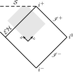
Figure 1: The computational domain (marked gray) on the background of the Carter-Penrose diagram of the Schwarzschild spacetime. The central spacelike singularity along $r=0$ and the event horizon are denoted as $\mathcal{S}$ and $\mathcal{EH}$, respectively. $\mathscr{I}^{\pm}$ and $i^{\pm}$ are null and timelike infinities, while $i^{0}$ is a spacelike infinity.

3.1 Initial data and evolution parameters

The only arbitrary initial conditions of the process were the field profiles posed on the initial $u=const.$ hypersurface. The profile of the evolving complex field was

$$\phi\left(v\right)=\frac{A}{\sqrt{8\pi}}\sin^{4}\left(\pi\frac{v-v_{i}}{v_{f}-v_{i}}\right)\left[\cos\left(2\pi\frac{v-v_{i}}{v_{f}-v_{i}}\right)+i\cos\left(2\pi\frac{v-v_{i}}{v_{f}-v_{i}}-\pi\delta\right)\right]$$ (31)

within the range $v_{i}\leqslant v\leqslant v_{f}$, where $v_{i}$ and $v_{f}$ were equal to $0$ and $20$, respectively, and was equal to zero outside the specified range of advanced time. Due to the fact that the field function is non-zero within the closed interval of advanced time, the spacetime region from within the specified range will be referred to as dynamical. The parameter $\delta$ takes values from the range $[0,0.5]$ and when it vanishes the evolving field $\phi$ can be interpreted as a real scalar field. The value of the amplitude $A$ responsible for the field gravitational self-interaction strength was set as equal to $0.25$. The effective gravitational constant $G=\Phi^{-1}$ was assumed to be equal to unity asymptotically and for this reason the initial profile of the Brans-Dicke field was set as

$$\Phi\left(v\right)=1.$$ (32)

The free evolution parameters $\beta$ and $\omega$ are model-dependent, while $\delta$, as was mentioned above, controls the type of the collapsing scalar field. The considered values of these constants and the corresponding theoretical models are the following.

• $\beta$: $0$ (type IIA model), $0.5$ (type I model), $1$ (heterotic model),

• $\omega$: $10$ (large $\omega$ limit), $0$ ($f(R)$ limit), $-1$ (dilatonic limit), $-1.4$ (brane-world limit), $-1.6$ (ghost limit),

• $\delta$: $0$ (real scalar field), $0.5$ (complex scalar field).

The adequate values of the free parameters will be given above each diagram presenting the collapse results.

Specific arguments for the above classification of the values of the constant $\beta$, which originate from a set of the string theory-inspired models, and the motivations for the studied values of $\omega$ are based on the classification of the full version of the string theory, which obviously involves terms of higher order in curvature and contains gauge fields Becker .

The expansions of the effective actions of the bosonic sector of the type IIA, type I and heterotic theories are

$$S_{\textrm{IIA}} = \frac{1}{2\lambda_{s}^{\,8}}\int d^{10}x\;\sqrt{-g}\;\Bigg{\{}e^{-\phi_{d}}\left[R+\big{(}\nabla\phi_{d}\big{)}^{2}-\frac{H_{3}^{\,2}}{12}\right]-\left(\frac{F_{2}^{\,2}}{4}+\frac{\tilde{F}_{4}^{\,2}}{48}\right)\Bigg{\}}+\cdots,$$ (33)

$$S_{\textrm{I}} = \frac{1}{2\lambda_{s}^{\,8}}\int d^{10}x\;\sqrt{-g}\;\Bigg{\{}e^{-\phi_{d}}\left[R+\big{(}\nabla\phi_{d}\big{)}^{2}\right]-\frac{\tilde{H}_{3}^{\,2}}{12}-e^{-\frac{\phi_{d}}{2}}\frac{\textrm{Tr}\big{(}F_{2}^{\,2}\big{)}}{4}\Bigg{\}}+\cdots,$$ (34)

$$S_{\textrm{het}} = \frac{1}{2\lambda_{s}^{\,8}}\int d^{10}x\;\sqrt{-g}\;e^{-\phi_{d}}\left[R+\big{(}\nabla\phi_{d}\big{)}^{2}-\frac{\tilde{\tilde{H}}_{3}^{\,2}}{2}-\frac{\textrm{Tr}\big{(}F_{2}^{\,2}\big{)}}{4}\right]+\cdots,$$ (35)

where $\lambda_{s}$ is the length scale of strings and $\phi_{d}$ denotes a dilaton field. $H_{3}$ is the field strength tensor of the NS-NS two-form $B_{2}$, while $\tilde{H}_{3}$ and $\tilde{\tilde{H}}_{3}$ stand for mixed contributions of the R-R two-form $A_{2}$ and the NS-NS two-form $B_{2}$, respectively, and the matrix-valued one-form $A_{1}$. $F_{2}$ is the field strength tensor of the R-R one-form $A_{1}$ and $\tilde{F}_{4}=dA_{3}+A_{1}\land H_{3}$ with $A_{3}$ being a three-form field. The dimensional reduction procedure results in the effective actions for the considered theories, which can be collectively written in the following form:

$$S_{\textrm{IIA/I/het}}^{(4)}=\frac{1}{16\pi}\int d^{4}x\;\sqrt{-g}\;\bigg{\{}e^{-\phi_{d}}\left[R+\big{(}\nabla\phi_{d}\big{)}^{2}\right]-{\mathchoice{\raisebox{0.0pt}{$\displaystyle\chi$}}{\raisebox{0.0pt}{$\textstyle\chi$}}{\raisebox{0.0pt}{$\scriptstyle\chi$}}{\raisebox{0.0pt}{$\scriptscriptstyle\chi$}}}F_{2}^{\,2}\bigg{\}}+\cdots,$$ (36)

where $\textstyle\chi$ equals $1$ for the type IIA, $e^{-\frac{\phi_{d}}{2}}$ for the type I and $e^{-\phi_{d}}$ for the heterotic theory. The redefinition of the dilaton field $e^{-\phi_{d}}\to\Phi_{d}$ leads to the gravitational sector, which is identical for all the examined versions of the string theory and proportional to the term $\Phi_{d}\Big{[}R+\big{(}\nabla\Phi_{d}\big{)}^{2}\Phi_{d}^{\>-2}\Big{]}$. The two-form field becomes proportional to the term $\Phi_{d}^{\>\beta}F_{2}^{\,2}$ with $\beta$ equal to $0$ for the type IIA, $0.5$ for the type I and $1$ for the heterotic theory. The obtained couplings provided an inspiration for the values of the Brans-Dicke field – matter sector coupling for the theoretical setup studied in the current paper.

The large $\omega$ limit was identified with the Brans-Dicke coupling equal to $10$, because for its larger values the behavior of the system does not change qualitatively. The gravitational sector of the action which corresponds to the scalar-tensor version of the $f(R)$ gravity is

$$S_{f(R)}=\frac{1}{16\pi}\int d^{4}x\;\sqrt{-g}\;\Big{[}f(\psi)+f^{\prime}(\psi)\left(R-\psi\right)\Big{]},$$ (37)

where $\psi$ is an auxiliary scalar field SotiriouFaraoni2010-451 . The field redefinition $f^{\prime}(\psi)\to\Phi_{\psi}$ allows to write the above action in the form

$$S_{f(R)}=\frac{1}{16\pi}\int d^{4}x\;\sqrt{-g}\;\Big{(}\Phi_{\psi}R-V(\Phi_{\psi})\Big{)},$$ (38)

which corresponds to a Brans-Dicke field with potential when the coupling vanishes. Thus, the case of $\omega=0$ was interpreted as the $f(R)$ limit of the theory. The low energy effective action of each string theory contains a sector with the dilaton field

$$S_{\textrm{d}} = \frac{1}{2\lambda_{s}^{\,D-1}}\int d^{D+1}x\;\sqrt{-g}\;e^{-\phi_{d}}\left[R+\big{(}\nabla\phi_{d}\big{)}^{2}\right],$$ (39)

where $D$ denotes the number of space dimensions Gasperini . The field redefinition $\lambda_{s}^{\,1-D}\cdot e^{-\phi_{d}}\to\Phi_{d}\left(8\pi G_{D-1}\right)^{-1}$, where $G_{D-1}$ is the $D-1$-dimensional gravitational constant, gives the $\omega=-1$ limit of the Brans-Dicke theory, which was called dilatonic. The value of the Brans-Dicke parameter can be calculated in the weak field limit of the Randall-Sundrum braneworld model RandallSundrum1999-3370 according to

$$\omega=\frac{3}{2}\left(e^{\pm\frac{s}{l}}-1\right),$$ (40)

where $s$ is the distance between the branes and $l=\sqrt{-6\Lambda^{-1}}$ denotes the length scale of the anti-de Sitter space, while the sign in the exponent depends on the sign of the brane tension GarrigaTanaka2000-2778 . The value of $\omega$ in these models is usually close to $-1.5$. The value $-1.4$ chosen for our computations thus represents the brane-world limit. When $\omega$ is less than $-1.5$, the kinetic term of the Brans-Dicke field in the Lagrangian is negative in the Einstein frame and hence the field acts as a ghost KimLeeLeeLeeYeom2011-023519 . The value of $-1.6$ was chosen as an example to investigate such an exotic behavior.

3.2 Penrose and field diagrams

The outcomes of the studied evolutions will be presented through the prism of causal structures of spacetimes and the behavior of fields in emerging dynamical spacetimes. The spacetime structures will be depicted on Penrose diagrams, which present the $r=const.$ lines in the $(vu)$-plane. On all plots of $r$-contours, the values of $r$ range from $0$ to $40$ and the differences between adjacent $r=const.$ lines are $\Delta r=1$. The central singularity situated along the $r=0$ line is marked as a thick black line. Apparent horizons located along the hypersurfaces of a vanishing expansion $r_{,v}=0$ and $r_{,u}=0$ are denoted as red and blue curves, respectively. Cauchy horizons, that is null hypersurfaces beyond which the evolution cannot be extended using the data from the previous time slice, are marked as green lines. The Penrose diagrams obtained during the numerical simulations are related via a conformal transformation to the Carter-Penrose diagrams, which depict the global structure of spacetimes and picture the causal relations within their distinct regions. The Carter-Penrose diagrams of the spacetimes formed in the examined process will be also presented.

The behavior of fields will be interpreted on the basis of the field functions values in the spacetime. Since one of the aims of the current studies is to assess a possibility of measuring time intrinsically, that is with the use of the fields comprising the examined dynamical system, the contours of constancy hypersurfaces will also be depicted. The spacetime regions in which the constant field function hypersurfaces are spacelike will be marked blue on the plots, while the areas in which they are timelike will be marked purple. The values of field functions covered by the computations and the adequate steps between the field constancy hypersurfaces are the following.

• For $\omega>-1.5$, the Brans-Dicke field ranges from $\Phi=0.1$ to $\Phi=1$ and the step $\Delta\Phi$ equals $0.01$.

• For $\omega>-1.5$, the real part of the complex scalar field ranges from $\phi_{Re}=-1$ to $\phi_{Re}=0.5$ with the step $\Delta\phi_{Re}=0.03$.

• For $\omega<-1.5$, the range of the Brans-Dicke field is $\Phi=1$ to $\Phi=20.9$ and the step between adjacent contours is $\Delta\Phi=0.2$.

• For $\omega<-1.5$, the real part of the complex scalar field ranges from $\phi_{Re}=-2.5$ to $\phi_{Re}=0.5$ and $\Delta\phi_{Re}$ is equal to $0.02$.

The asymptotic regions and areas neighboring the central singularity in the dynamical part of a spacetime were magnified for several selected diagrams. In these cases the field function contours were plotted more densely and the values of steps were placed in captions of adequate figures in section 5.

The Lagrangian of the complex scalar field (2) has a continuous global symmetry, which rotates the real and imaginary parts of the field (or, equivalently, changes the field phase, $\phi\to e^{i\vartheta}\phi$, where $\vartheta$ is the phase angle). The derived equation of motion (7) is also invariant, so no physical differences in the behavior of the real and imaginary parts of the complex scalar field are expected during the evolution. For this reason only the behavior of the real field component was shown on the plots.

4 Structures of spacetimes

The structures of spacetimes resulting from the gravitational collapse of real and complex scalar fields in the Brans-Dicke theory are presented in figures 2, 3 and 4 for the coupling constant $\beta$ equal to $0$, $0.5$ and $1$, respectively.

4.1 Uncoupled Brans-Dicke and scalar fields

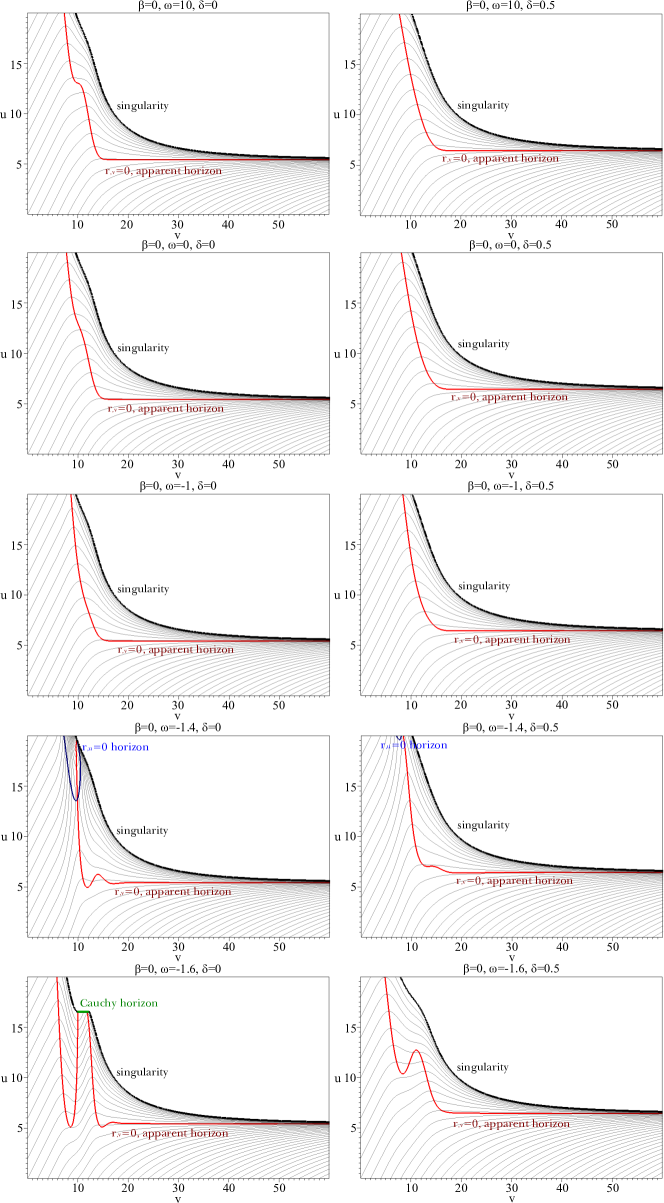
Figure 2: (color online) The Penrose diagrams of spacetimes formed during evolutions of real and complex scalar fields in the regime of the Brans-Dicke theory for $\beta=0$.

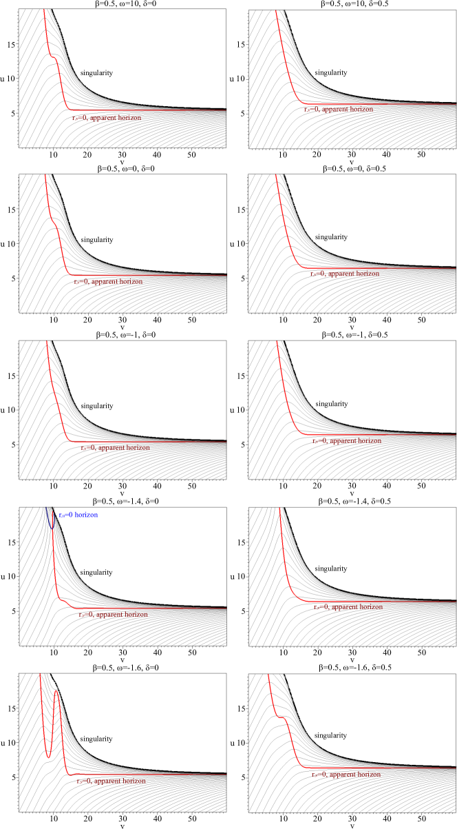
Figure 3: (color online) The Penrose diagrams of spacetimes formed during evolutions of real and complex scalar fields in the regime of the Brans-Dicke theory for $\beta=0.5$.

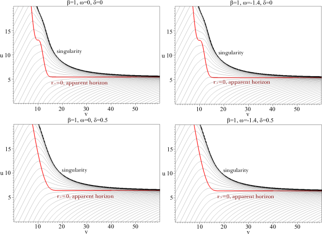
Figure 4: (color online) The Penrose diagrams of spacetimes formed during evolutions of real and complex scalar fields in the regime of the Brans-Dicke theory for $\beta=1$.

In the uncoupled case, i.e., for $\beta=0$, the spacetimes formed during the evolution of both real and complex scalar fields for $\omega$ equal to $10$, $0$ and $-1$ contain a spacelike singularity along $r=0$, which is surrounded by a single apparent horizon $r_{,v}=0$. The horizon hypersurface is spacelike at early advanced times and becomes null as $v\to\infty$ where the collapse dynamics settles at a final stationary state. The described structure is also a result of the gravitational collapse of a neutral scalar field proceeding in Einstein gravity HamadeStewart1996-497 , the collapse of an electrically charged scalar field in dilaton gravity BorkowskaRogatkoModerski2011-084007 ; NakoniecznaRogatko2012-3175 and the gravitational evolution of a complex scalar field coupled with phantom Maxwell field NakoniecznaRogatkoModerski2012-044043 or with a non-phantom Maxwell field and a complex scalar field with a quartic potential charged under a U(1) gauge field NakoniecznaRogatkoNakonieczny2015-012 within general relativity. For $\omega=-1.4$ the spacetime which stems from the investigated evolution contains a central spacelike singularity encompassed by an apparent horizon $r_{,v}=0$, which can be either spacelike or timelike in the dynamical region of the spacetime and is located along a null hypersurface $u=const.$ for large advanced times. There also exists another horizon in the spacetime, which is situated at the $r_{,u}=0$ hypersurface and forms at late retarded times in the dynamical region of the spacetime. In the ghost limit, for $\omega$ equal to $-1.6$, the emerging structures differ for real and complex scalar fields. In the case of $\delta=0$, there are two portions of a central spacelike singularity. They are separately surrounded by the $r_{,v}=0$ apparent horizons, which are spacelike or timelike in the spacetime area, in which the collapse dynamics takes place. As in all previous cases, the apparent horizon changes its character to null as $v\to\infty$. The two parts of the singularity mentioned above are linked by a Cauchy horizon null segment, which is not surrounded by any apparent horizon and thus can be visible for a distant observer. This violation of the weak cosmic censorship conjecture is due to the violation of the energy conditions in the ghost limit. When the parameter $\delta$ equals $0.5$, the spacetime contains a spacelike singularity along $r=0$. It is surrounded by a single apparent horizon which is either spacelike or timelike in the region related to the field dynamics and settles along $u=const.$ hypersurface at large advanced times. The results obtained for the real scalar field in the type IIA inspired model are in agreement with previous findings presented in HwangYeom2010-205002 .

4.2 Coupled Brans-Dicke and scalar fields

The course and outcomes of the studied process in the type I inspired model, that is for $\beta=0.5$, are qualitatively similar to the above-mentioned case of the vanishing coupling between the Brans-Dicke field and the scalar field. The only difference can be noted when $\omega$ equals $-1.4$ and $-1.6$, because in contrast to the $\beta=0$ case, the apparent horizon $r_{,u}=0$ and the Cauchy horizon do not form in the spacetime at late retarded time when $\beta$ takes the value of $0.5$ for $\delta$ equal to $0.5$ and $0$, respectively.

When $\beta$ is equal to $1$, the spacetimes formed during the examined process for all values of the Brans-Dicke coupling constant $\omega$ have similar structures. The intrinsic spacelike singularity at $r=0$ is surrounded by an apparent horizon $r_{,v}=0$, which is spacelike for small advanced times and becomes null as $v\to\infty$. There exists one dissimilarity between the evolutions of real and complex scalar fields. In the case of vanishing $\delta$, the spacelike part of the horizon passes directly to the null part, while when $\delta=0.5$ there is an intermediate stage, in which the horizon is timelike for medium values of advanced time.

4.3 Overall dependence on the evolution parameters

In general, the variety and complexity of the spacetime structures formed during the gravitational evolution of a scalar field in the Brans-Dicke theory decrease as the value of the coupling constant $\beta$ between the Brans-Dicke field and the scalar field increases. Moreover, the model dependence reflected in the values of the Brans-Dicke coupling $\omega$ indicates that the collapse of a scalar field in the large $\omega$, $f(R)$ and dilatonic limits proceeds similarly to the same process in the Einstein gravity. In the brane-world limit additional apparent horizons are possible at late times, while the ghost limit enables the formation of more exotic structures, such as these in which the weak cosmic censorship can be violated. A summary of causal structures of spacetimes obtained as a result of the examined collapse is presented in figure 5 in the form of Carter-Penrose diagrams.

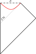
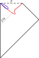
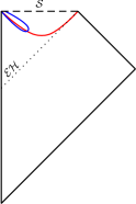
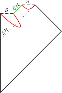
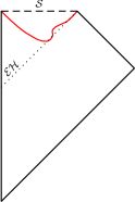
Figure 5: (color online) The Carter-Penrose diagrams of spacetimes formed during evolutions of a scalar field in the Brans-Dicke theory, for the following sets of evolution parameters: (a) $\omega\geqslant-1$ for $\beta=0$, $0.5$ and $\beta=1$, $\delta=0$, (b) $\beta=0$, $0.5$, $\omega=-1.4$, $\delta=0$, (c) $\beta=0$, $\omega=-1.4$, $\delta=0.5$, (d) $\beta=0$, $\omega=-1.6$, $\delta=0$, (e) $\beta=0$, $\omega=-1.6$, $\delta=0.5$ and $\beta=0.5$, $\omega=-1.6$ and (f) $\beta=0.5$, $\omega=-1.4$, $\delta=0.5$ and $\beta=1$, $\delta=0.5$. The central singularity along $r=0$, the event and Cauchy horizons are denoted as $\mathcal{S}$, $\mathcal{EH}$ and $\mathcal{CH}$, respectively.

5 Dynamical behavior of fields

The evolution of the Brans-Dicke and complex scalar fields (6)–(7) in double null coordinates is governed by the following equations:

$$\Phi_{,uv} = -\frac{fZ+gW}{r}-\frac{\Phi^{\beta}\left(1-\beta\right)}{3+2\omega}\left(w\bar{z}+z\bar{w}\right),$$ (41)

$$\phi_{,uv} = -\frac{fz+gw}{r}-\frac{\beta}{2\Phi}\left(Wz+Zw\right).$$ (42)

As may be inferred from (41), the case of $\omega=-1.5$ is a singular point of the evolution equation. The dynamical behavior of the Brans-Dicke field when it approaches the central singularity depends on the value of the parameter $\omega$. For $\omega>-1.5$, the Brans-Dicke field moves toward $\Phi=0$ nearby the singularity, i.e., it is biased toward the strong coupling limit. Conversely, for $\omega<-1.5$, it tends to $\Phi=\infty$ as it evolves toward the singularity, which means that it is biased toward the weak coupling limit.

5.1 Type IIA and type I models

Figures 6 and 7 present the hypersurfaces of constant Brans-Dicke field and the scalar field, respectively, in spacetimes formed during evolutions conducted for $\beta=0$. The enlarged dynamical and asymptotic regions of the vicinity of the central singularity are shown in figure 8. The constant Brans-Dicke field and scalar field hypersurfaces in the spacetimes which stem from the gravitational collapse for $\beta=0.5$ are shown in figures 9 and 10, respectively. The selected asymptotic regions neighboring the central singularity were enlarged and are depicted in figure 11.

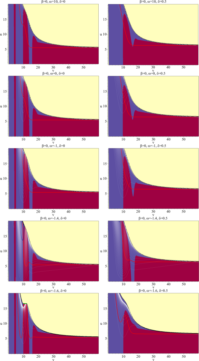
Figure 6: (color online) The constancy hypersurfaces of the Brans-Dicke field for evolutions conducted within the Brans-Dicke theory for $\beta=0$.

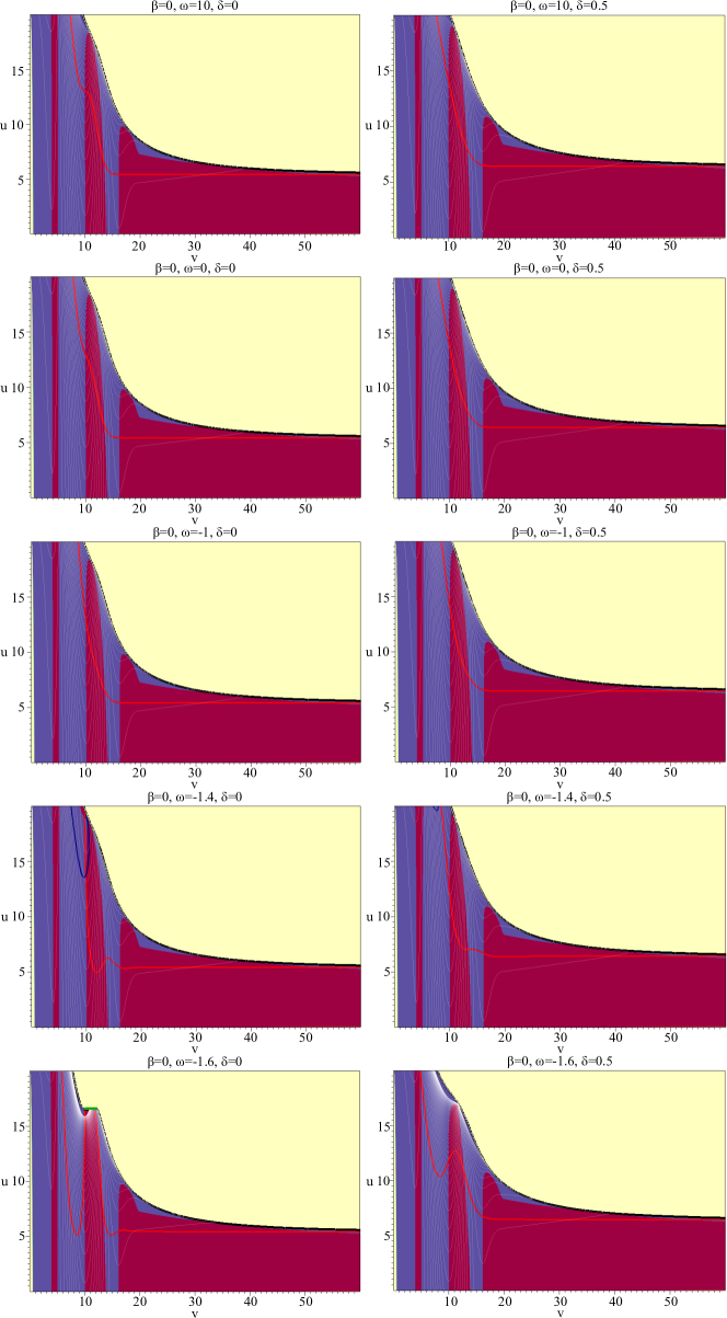
Figure 7: (color online) The contours of the real part of the complex scalar field for evolutions conducted within the Brans-Dicke theory for $\beta=0$.

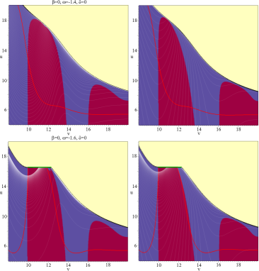
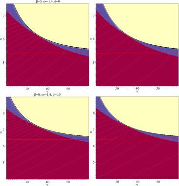
Figure 8: (color online) Field contours in (a) the dynamical region and (b) the asymptotic region of spacetimes formed in the collapse within the Brans-Dicke theory for $\beta=0$. Left column: the Brans-Dicke field. Right column: the real part of the complex scalar field. The steps between the contours are $\Delta\Phi=0.0025$ and $\Delta\phi_{Re}=0.002$.

The dynamics of the Brans-Dicke field depends on both parameters $\omega$ and $\delta$ in the cases of $\beta$ equal to $0$ and $0.5$. It is especially clear for spacetimes obtained with $\omega\geqslant-1.4$, for which the field varies more substantially and at earlier retarded times as $\omega$ decreases. The most considerable field dynamics is observed at late retarded times nearby the singularity. In the ghost limit, i.e., for $\omega=-1.6$, the field function varies extensively in the vicinity of the Cauchy horizon, which is the limit of predictability of the evolution equations. The influence of the parameter $\delta$ on the Brans-Dicke field dynamics is far less apparent in comparison to $\omega$. In the case of the evolution proceeding in the presence of the real scalar field, the variations of the Brans-Dicke field function are slightly smaller in comparison to the ones observed during evolutions with $\delta=0.5$.

A spacelike character of the hypersurfaces along which the Brans-Dicke field is constant is manifested in the regions of high curvature, that is nearby the central singularity, in all dynamical spacetimes. There exist separated points, at which the $r=0$ singularity seems to have one common point with the regions of spacelike lines of constant Brans-Dicke field. In the case of $\delta=0$, such points exist along the whole central singularity, while for the complex scalar field they appear only in the asymptotic region, that is for large values of advanced time. It means that the presence of a complex scalar field is conducive to measuring time with the use of the accompanying Brans-Dicke field, especially in the dynamical spacetime region. The exact determination whether in these points single null or timelike constancy hypersurfaces reach the singularity is impossible because of the limitations associated with conducting numerical calculations nearby the singularity. However, even if such isolated points do exist, they do not influence the usefulness of the Brans-Dicke field in time quantification in the vicinity of the singularity. A similar situation was also observed for a gravitationally collapsing single real scalar field in Einstein gravity NakoniecznaLewandowski2015-064031 . The lines indicating equal values of the Brans-Dicke field function in the spacetime are timelike in the vicinity of the Cauchy horizon, which forms when $\omega$ equals $-1.6$, so in this spacetime region the field definitely cannot be used as a time measurer. It should be emphasized that a potential time measuring with the use of the Brans-Dicke field in the considered theoretical setup nearby the singularity is possible also due to the fact that the field constancy hypersurfaces vary monotonically in this area.

The behavior of the hypersurfaces of constant values of the scalar field function is uniform for $\omega\geqslant-1.4$ with only minor differences for the two investigated values of the parameter $\delta$. The scalar field is certainly more dynamical in the case of $\omega=-1.6$ in the neighborhood of the Cauchy horizon and the central singularity at late retarded times. The field constancy hypersurfaces are spacelike in the vicinity of the singularity and only isolated points at the singularity in which they may potentially be non-spacelike exist, similarly to the case of the Brans-Dicke field described above. The timelike character of the hypersurfaces is observed nearby the Cauchy horizon and for this reason the scalar field cannot serve as a time measurer there. The changes of the field function values are monotonic as the singularity is approached, which is also a necessary condition in order to quantify time using the evolving scalar field.

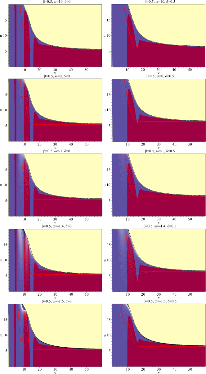
Figure 9: (color online) The constancy hypersurfaces of the Brans-Dicke field for evolutions conducted within the Brans-Dicke theory for $\beta=0.5$.

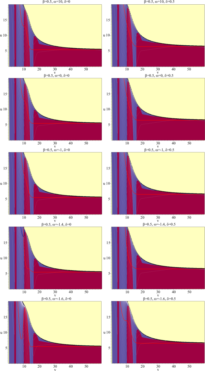
Figure 10: (color online) The contours of the real part of the complex scalar field for evolutions conducted within the Brans-Dicke theory for $\beta=0.5$.

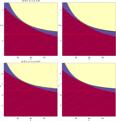
Figure 11: (color online) Field contours in the asymptotic region of spacetimes formed in the collapse within the Brans-Dicke theory for $\beta$ equal to $0.5$. Left column: the Brans-Dicke field. Right column: the real part of the complex scalar field. The steps between the contours are $\Delta\Phi=0.0025$ and $\Delta\phi_{Re}=0.002$.

5.2 Heterotic model

When $\beta$ equals $1$, the evolution equation of the Brans-Dicke field (41) reduces to the homogeneous wave equation written in double null coordinates. Thus, the initially constant field function remains unchanged within the whole computational domain. For this reason, the Brans-Dicke field cannot be used as a time variable in this case. The hypersurfaces of the constant scalar field function in the case of $\beta=1$ are presented in figure 12. It turns out that the scalar field dynamics does not depend on the evolution parameters. As in the previous cases, the monotonicity of the field function is observed in the region of high curvature near the central singularity. The field constancy hypersurfaces are also spacelike in this region, apart from single separated points, in which a timelike or null hypersurface can potentially reach the central $r=0$ singular line. Due to the above arguments, although the Brans-Dicke field is excluded as a clock in the heterotic theory, the scalar field remains a good candidate in this regard.

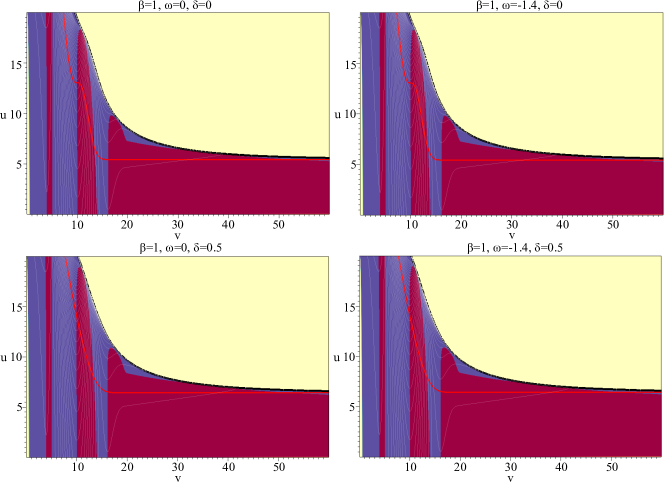
Figure 12: (color online) The contours of the real part of the complex scalar field for evolutions conducted within the Brans-Dicke theory for $\beta=1$.

5.3 Overall dependence on the evolution parameters

When the influence of the $\beta$ coupling constant on the overall field dynamics during the collapse is considered, it turns out that there are no conspicuous differences between the process proceeding within the type IIA and type I models. Significant distinctness is observed for $\beta=1$, i.e., in the heterotic theory, mainly due to the fact that the equation of motion of the Brans-Dicke field (41) simplifies as was described above and the field dynamics becomes trivial. The parameter $\omega$ strongly influences the behavior of the Brans-Dicke field, whose dynamics is most significant for $\omega$ close to $-1.5$, while its impact on the scalar field dynamics is unnoticeable.

6 Conclusions

The dynamical gravitational collapse of complex and real scalar fields in the Brans-Dicke theory was investigated. The structures of the emerging spacetimes were examined and the feasibility of performing time measurements with the use of evolving scalar fields during dynamical processes driven by the gravitational interaction was assessed. Several values of the Brans-Dicke coupling constant, which corresponded to the large $\omega$, $f(R)$, dilatonic, brane-world and ghost limits, were investigated. The studied coupling between the Brans-Dicke field and the matter sector of the theory, which was controlled by the $\beta$ parameter, was motivated by the type IIA, type I and heterotic string theory-inspired models.

In the case of $\omega$ equal to $10$, $0$ and $-1$ in the type IIa and type I models, as well as for all its values within the heterotic model, in the spacetimes which stem from the collapse of both real and complex scalar fields there exists a spacelike central singularity surrounded by a single apparent horizon. When $\beta=0$ and the Brans-Dicke coupling equals $-1.4$, an additional horizon appears in the spacetime at late retarded times. It is absent in the case of $\beta=0.5$ and $\omega=-1.4$, $\delta=0.5$. During the collapse of a real scalar field with $\beta=0$ and $\omega=-1.6$, two parts of a spacelike central singularity surrounded separately by the apparent horizons form. They are linked by a Cauchy horizon null segment, which is visible for a distant observer. During the collapse of a complex scalar field, the emerging spacetime contains a spacelike singularity along $r=0$, which is situated beyond a single apparent horizon. In all the cases, the apparent horizon settles along the $u=const.$ hypersurface as $v\to\infty$, i.e., in the non-dynamical part of the spacetime.

When $\beta$ equals $0$ and $0.5$, the Brans-Dicke field dynamics is more considerable at earlier retarded times as $\omega$ decreases. The values of the field function vary most significantly in the vicinity of the central singularity and nearby the Cauchy horizon, if it exists in the spacetime. The variations of the Brans-Dicke field function are slightly smaller when it is accompanied by the real scalar field, when compared with the evolution proceeding in the presence of a complex scalar field. The case of $\beta=1$ excludes the Brans-Dicke field from being treated as a time variable, because due to the form of its evolution equation, it remains constant within the whole dynamical spacetime.

In all dynamical spacetimes obtained in type IIa and type I models the constancy hypersurfaces of the Brans-Dicke field are spacelike nearby the central singularity. There are several points, at which a non-spacelike hypersurface can potentially reach the singularity. However, due to the fact that these points are separated, they do not prevent the field from acting as a time measurer. The constancy hypersurfaces of the Brans-Dicke field are timelike nearby the Cauchy horizon and hence they cannot serve as ‘clocks’ there. The potential usefulness of the Brans-Dicke field for time measurements nearby the singularity is possible also due to the fact that the field constancy hypersurfaces vary monotonically in this area.

In the cases of $\beta$ equal to $0$ and $0.5$, the behavior of the scalar field function constancy hypersurfaces displays only minor differences for the two investigated values of the parameter $\delta$. The scalar field dynamics is most noticeable in the neighborhood of the Cauchy horizon and the central singularity at late retarded times. The hypersurfaces of constant field function are spacelike in the vicinity of the singularity and only isolated points at the singularity in which they may potentially be non-spacelike exist. The timelike character of the hypersurfaces is observed nearby the Cauchy horizon and for this reason the scalar field cannot serve as a time measurer in this area. The changes of the field function values are monotonic as the singularity is approached. In the case of $\beta=1$, the scalar field dynamics does not depend on the evolution parameters and the above qualitative description applies also to this case. Although the Brans-Dicke field is excluded as a clock in the heterotic theory, the scalar field remains a good candidate in this regard.

In conclusion, using scalar fields as time variables within the whole evolving spacetime during dynamical gravitational evolutions of coupled matter-geometry systems encounters several obstacles, which can be problematic and should be remembered. First, the two conditions which are necessary for treating the field as a time measurer (spacelike character of its constancy hypersurfaces and monotonicity of their parametrization) are not fulfilled in the whole spacetime. Second, the vicinity of Cauchy horizons should be excluded from such analyses, at least within the studied theoretical setup. Third, the forms of the field evolution equations should be analyzed thoroughly for various values of parameters which they contain, because the possibility of using the specific scalar field as a time variable may be excluded in some cases. Fortunately, only the last of the outlined difficulties applies to a close proximity of the singularity emerging in the spacetime. This region of high curvature is of crucial importance from the viewpoint of gravity quantization, which is the main reason of the undertaken studies. Hence, the scalar fields can be used to quantify time nearby the spacetime singularity (provided that the equation of motion of the particular field does not reduce to the wave equation and thus the values of the field functions vary there).

The investigated case was the neutral gravitational collapse. There exists a question whether additional gauge vector field can influence the obtained results and either strengthen or weaken the conclusion that both real and complex scalar fields can be used as time variables during dynamical evolutions of coupled matter-geometry systems. Since the studied process proceeding in the presence of an electric charge is a toy-model for the realistic collapse HodPiran1998-1554 ; HodPiran1998-1555 ; SorkinPiran2001-084006 ; SorkinPiran2001-124024 ; OrenPiran2003-044013 , we plan to address this issue in the future researches. It will also allow us to investigate the regions neighboring Cauchy horizons in more detail, as these null hypersurfaces appear naturally during the charged collapse.

Appendix A Numerical computations

The scheme employed in the numerical simulations was described in detail in HansenKhokhlovNovikov2005-044013 ; DoroshkevichHansenNovikovNovikovParkShatskiy2010-124011 ; HongHwangStewartYeom2010-045014 ; HwangYeom2011-064020 ; HansenLeeParkYeom2013-235022 ; HwangYeom2010-205002 ; HansenYeom2014-040 ; HansenYeom2015-019 . The initial conditions were imposed on a set of dynamical variables ($\alpha$, $h$, $d$, $r$, $f$, $g$, $\Phi$, $W$, $Z$, $s$, $w$, $z$) on two null $u=const.$ and $v=const.$ hypersurfaces, which were assumed to be $u=0$ and $v=0$ for the need of the numerical setup. The gauge freedom of the $r$ function was fixed by imposing constant $r|_{(0,0)}$, $f|_{v=0}$ and $g|_{u=0}$, where the last two were negative and positive, respectively, so that the radial function decreased for an ingoing observer and increased for an outgoing one. The values of $Z$ and $z$ along $u=0$ stemmed from initial conditions (31) and (32). At the hypersurface $v=0$, the Brans-Dicke field was set as equal to unity and, due to the shell-shaped form of the scalar field, the function $s$ was constant and equal to $A$. The functions $W$ and $w$ were thus also specified. The metric function $\alpha$ was equal to $1$ which gave $h=0$ at $v=0$, since this axis was not affected by the evolving scalar field in the form of a shell. The remaining initial conditions were calculated with the use of the above foundations and appropriate equations from among the set (27)–(30).

The correctness of the numerical code was checked using a sample evolution described by parameters $\beta=0$, $\omega=-1$ and $\delta=0.5$. The constraints were monitored during the process using the following equations:

$$\textrm{Eq}_{1} \equiv \frac{r_{,uu}-2fh+4\pi r\left(T_{uu}^{\Phi}+T_{uu}^{\mathrm{M}}\Phi^{-1}\right)}{|r_{,uu}|+|2fh|+4\pi r\left(\left|T_{uu}^{\Phi}\right|+\left|T_{uu}^{\mathrm{M}}\Phi^{-1}\right|\right)},$$ (43)

$$\textrm{Eq}_{2} \equiv \frac{r_{,vv}-2gd+4\pi r\left(T_{vv}^{\Phi}+T_{vv}^{\mathrm{M}}\Phi^{-1}\right)}{|r_{,vv}|+|2gd|+4\pi r\left(\left|T_{vv}^{\Phi}\right|+\left|T_{vv}^{\mathrm{M}}\Phi^{-1}\right|\right)}.$$ (44)

The above relations as functions of advanced time calculated for three selected values of retarded time are shown in figure 13. In both cases these should be zero in principle and the deviations appear due to numerical errors. There are two regions in which the values rise considerably, i.e., for small values of $v$ due to the fact that the denominators are very close to zero and nearby the singularity. As can be inferred from the plot, except a close neighborhood of the singularity, the errors do not exceed $0.1\%$. Since the constraint equations are stable, the simulations are consistent.

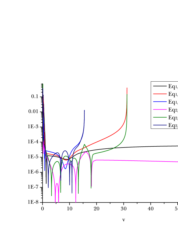
Figure 13: (color online) Monitoring of the constraints. The values of the equations (43) and (44) were calculated along three null hypersurfaces of constant $u$ equal to $2.5$, $7.5$ and $12.5$.

The convergence of the code was checked and the outcome is presented in figure 14. The values of a quantity constructed from the $r$ function obtained on two grids with a quotient of integration steps equal to $2$ were calculated along three arbitrarily chosen $u=const.$ lines. An overlap between two profiles of the defined quantity at each $u=const.$ was obtained when the result from finer grids was multiplied by $4$. Thus, the code displays a second order convergence. The discrepancy between each two profiles at the constant $u$ is less than $0.01\%$ except a close vicinity of the singularity. Hence, the coarsest grid was adequate for performing the simulations.

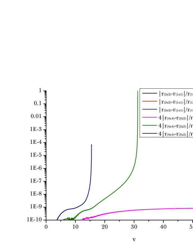
Figure 14: (color online) The convergence of the code presented through the prism of the values of the quantity $|r_{(2k\times 2k)}-r_{(k\times k)}|/r_{(k\times k)}$ with $k=1,2$ calculated at the same hypersurfaces of constant $u$ as in figure 13. $(k\times k)$ denotes the resolution of the numerical grid, on which the computations were conducted.

- (1) B. S. DeWitt, Quantum theory of gravity. I. The canonical theory, Phys. Rev. 160 (1967) 1113.
- (2) C. Rovelli, Time in quantum gravity: An hypothesis, Phys. Rev. D 43 (1991) 442.
- (3) C. Rovelli and L. Smolin, The physical hamiltonian in nonperturbative quantum gravity, Phys. Rev. Lett. 72 (1994) 446.
- (4) M. Domagała, K. Giesel, W. Kamiński, and J. Lewandowski, Gravity quantized: Loop quantum gravity with a scalar field, Phys. Rev. D 82 (2010) 104038.
- (5) J. Lewandowski, M. Domagała, and M. Dziendzikowski, The dynamics of the massless scalar field coupled to LQG in the polymer quantization, Proc. Sci. QGQGS 2011 (2012) 025.
- (6) S. Alexander, J. Malecki, and L. Smolin, Quantum gravity and inflation, Phys. Rev. D 70 (2004) 044025.
- (7) A. Ashtekar, T. Pawłowski, and P. Singh, Quantum nature of the big bang, Phys. Rev. Lett. 96 (2006) 141301.
- (8) A. Ashtekar, T. Pawłowski, and P. Singh, Quantum nature of the big bang: Improved dynamics, Phys. Rev. D 74 (2006) 084003.
- (9) M. Da̧browski and A. L. Larsen, Quantum Tunneling Effect in Oscillating Friedmann Cosmology, Phys. Rev. D 52 (1995) 3424.
- (10) P. W. Graham, B. Horn, S. Kachru, S. Rajendran, and G. Torroba, A simple harmonic universe, JHEP 1402 (2014) 029.
- (11) A. T. Mithani and A. Vilenkin, Collapse of simple harmonic universe, JCAP 01 (2012) 028.
- (12) A. T. Mithani and A. Vilenkin, Tunneling decay rate in quantum cosmology, Phys. Rev. D 91 (2015) 123511.
- (13) L. Perlov, Wheeler–DeWitt equation for 4D supermetric and ADM with massless scalar field as internal time, Phys. Lett. B 743 (2015) 143.
- (14) J. D. Brown and K. V. Kuchar, Dust as a standard of space and time in canonical quantum gravity, Phys. Rev. D 51 (1995) 5600.
- (15) X. Zhang, M. Artymowski, and Y. Ma, Loop quantum Brans-Dicke cosmology, Phys. Rev. D 87 (2013) 084024.
- (16) C. R. Almeida, A. B. Batista, J. C. Fabris, and P. R. L. V. Moniz, Quantum cosmology with scalar fields: self-adjointness and cosmological scenarios, Gravit. Cosmol. 21 (2015) 191.
- (17) C. Brans and R. H. Dicke, Mach’s Principle and a Relativistic Theory of Gravitation, Phys. Rev. 124 (1961) 925–935.
- (18) V. Faraoni, Illusions of general relativity in Brans-Dicke gravity, Phys. Rev. D 59 (1999) 084021.
- (19) C. M. Will, The Confrontation between General Relativity and Experiment, Living Rev. Relativity 17 (2014) 4.
- (20) C. Romero and A. Barros, Does the Brans-Dicke theory of gravity go over to general relativity when ?, Physics Letters A 173 (1993) 243–246.
- (21) B. Chauvineau, On the limit of Brans–Dicke theory when , Classical and Quantum Gravity 20 (2003) 2617.
- (22) B. Chauvineau, A. D. A. M. Spallicci, and J.-D. Fournier, Brans–Dicke gravity and the capture of stars by black holes: some asymptotic results, Classical and Quantum Gravity 22 (2005) S457.
- (23) B. Chauvineau, Stationarity and large Brans–Dicke solutions versus general relativity, General Relativity and Gravitation 39 (2007) 297–306.
- (24) Bertotti B., Iess L., and Tortora P., A test of general relativity using radio links with the Cassini spacecraft, Nature 425 (2003) 374–376.
- (25) A. De Felice, G. Mangano, P. D. Serpico, and M. Trodden, Relaxing nucleosynthesis constraints on Brans-Dicke theories, Phys. Rev. D 74 (2006) 103005.
- (26) J. Fabris, S. Goncalves, and R. d. S. Ribeiro, Late time accelerated Brans-Dicke pressureless solutions and the supernovae type Ia data, Grav. Cosmol. 12 (2006) 49–54.
- (27) L.-e. Qiang, Y. Gong, Y. Ma, and X. Chen, Cosmological implications of 5-dimensional Brans–Dicke theory, Physics Letters B 681 (2009) 210–213.
- (28) O. Hrycyna, M. Szydłowski, and M. Kamionka, Dynamics and cosmological constraints on Brans-Dicke cosmology, Phys. Rev. D 90 (2014) 124040.
- (29) A. Avilez and C. Skordis, Cosmological Constraints on Brans-Dicke Theory, Phys. Rev. Lett. 113 (2014) 011101.
- (30) Y.-C. Li, F.-Q. Wu, and X. Chen, Constraints on the Brans-Dicke gravity theory with the Planck data, Phys. Rev. D 88 (2013) 084053.
- (31) V. Acquaviva, C. Baccigalupi, S. M. Leach, A. R. Liddle, and F. Perrotta, Structure formation constraints on the Jordan-Brans-Dicke theory, Phys. Rev. D 71 (2005) 104025.
- (32) T. Damour and K. Nordtvedt, General relativity as a cosmological attractor of tensor-scalar theories, Phys. Rev. Lett. 70 (1993) 2217–2219.
- (33) T. Damour and K. Nordtvedt, Tensor-scalar cosmological models and their relaxation toward general relativity, Phys. Rev. D 48 (1993) 3436–3450.
- (34) T. Damour, F. Piazza, and G. Veneziano, Violations of the equivalence principle in a dilaton-runaway scenario, Phys. Rev. D 66 (2002) 046007.
- (35) D. La and P. J. Steinhardt, Extended Inflationary Cosmology, Phys. Rev. Lett. 62 (1989) 376.
- (36) C. Mathiazhagan and V. Johri, An inflationary universe in Brans-Dicke theory: a hopeful sign of theoretical estimation of the gravitational constant, Class. Quant. Grav. 1 (1998) 29.
- (37) M. Arik and M. C. Çalik, Primordial and late-time inflation in Brans–Dicke cosmology, Journal of Cosmology and Astroparticle Physics 2005 (2005) 013.
- (38) M. Arik, M. Çalik, and M. B. Sheftel, Friedmann equation for Brans-Dicke cosmology, International Journal of Modern Physics D 17 (2008) 225–235.
- (39) S. Sen and A. A. Sen, Late time acceleration in Brans-Dicke cosmology, Phys. Rev. D 63 (2001) 124006.
- (40) L.-e. Qiang, Y. Ma, M. Han, and D. Yu, Five-dimensional Brans-Dicke theory and cosmic acceleration, Phys. Rev. D 71 (2005) 061501.
- (41) J. P. de Leon, Late time cosmic acceleration from vacuum Brans–Dicke theory in 5D, Classical and Quantum Gravity 27 (2010) 095002.
- (42) J. P. de Leon, Brans-Dicke cosmology in 4D from scalar-vacuum in 5D, Journal of Cosmology and Astroparticle Physics 2010 (2010) 030.
- (43) Y. Bisabr, Cosmic acceleration in Brans–Dicke cosmology, General Relativity and Gravitation 44 (2012) 427–435.
- (44) Y. Bisabr, Chameleon Brans-Dicke cosmology, Phys. Rev. D 86 (2012) 127503.
- (45) L. L. Samojeden, F. P. Devecchi, and G. M. Kremer, Fermions in Brans-Dicke cosmology, Phys. Rev. D 81 (2010) 027301.
- (46) D.-J. Liu, Dynamics of Brans-Dicke cosmology with varying mass fermions, Phys. Rev. D 82 (2010) 063523.
- (47) S. Nojiri and S. Odintsov, Unifying phantom inflation with late-time acceleration: scalar phantom–non-phantom transition model and generalized holographic dark energy, General Relativity and Gravitation 38 1285–1304.
- (48) S. Capozziello, S. Nojiri, and S. Odintsov, Unified phantom cosmology: Inflation, dark energy and dark matter under the same standard, Physics Letters B 632 (2006) 597–604.
- (49) M. Setare, The holographic dark energy in non-flat Brans–Dicke cosmology, Physics Letters B 644 (2007) 99–103.
- (50) M. Setare and M. Jamil, Holographic dark energy in Brans–Dicke cosmology with chameleon scalar field, Physics Letters B 690 (2010) 1–4.
- (51) H. Farajollahi, J. Sadeghi, M. Pourali, and A. Salehi, Stability analysis of agegraphic dark energy in Brans–Dicke cosmology, Astrophysics and Space Science 339 (2012) 79–85.
- (52) S. Chattopadhyay, A. Pasqua, and M. Khurshudyan, New holographic reconstruction of scalar-field dark-energy models in the framework of chameleon Brans–Dicke cosmology, The European Physical Journal C 74 (2014) 3080.
- (53) O. Hrycyna and M. Szydłowski, Dynamical complexity of the Brans-Dicke cosmology, Journal of Cosmology and Astroparticle Physics 2013 (2013) 016.
- (54) A. Paliathanasis, M. Tsamparlis, S. Basilakos, and J. D. Barrow, Classical and Quantum Solutions in Brans-Dicke Cosmology with a Perfect Fluid, arXiv:1511.00439 [gr-qc] (2015).
- (55) A. Einstein and E. G. Straus, The influence of the expansion of space on the gravitation fields surrounding the individual stars, Rev. Mod. Phys. 17 (1945) 120.
- (56) N. Sakai and J. D. Barrow, Cosmological evolution of black holes in Brans–Dicke gravity, Classical and Quantum Gravity 18 (2001) 4717.
- (57) M. Novello and S. P. Bergliaffa, Bouncing cosmologies, Physics Reports 463 (2008) 127–213.
- (58) J. C. Fabris, R. G. Furtado, P. Peter, and N. Pinto-Neto, Regular cosmological bouncing solutions in low energy effective action from string theories, Phys. Rev. D 67 (2003) 124003.
- (59) D. A. Tretyakova, A. A. Shatskiy, I. D. Novikov, and S. Alexeyev, Nonsingular Brans-Dicke- cosmology, Phys. Rev. D 85 (2012) 124059.
- (60) D. A. Tretyakova, B. N. Latosh, and S. O. Alexeyev, Wormholes and naked singularities in Brans–Dicke cosmology, Classical and Quantum Gravity 32 (2015) 185002.
- (61) M. Artymowski, Y. Ma, and X. Zhang, Comparison between Jordan and Einstein frames of Brans-Dicke gravity a la loop quantum cosmology, Phys. Rev. D 88 (2013) 104010.
- (62) A. Nakonieczna and J. Lewandowski, Scalar field as a time variable during gravitational evolution, Phys. Rev. D 92 (2015) 064031.
- (63) R. Torres and F. Fayos, Singularity free gravitational collapse in an effective dynamical quantum spacetime, Physics Letters B 733 (2014) 169–175.
- (64) R. Torres and F. Fayos, On the quantum corrected gravitational collapse, Physics Letters B 747 (2015) 245–250.
- (65) C. Vaz, Quantum gravitational dust collapse does not result in a black hole, Nuclear Physics B 891 (2015) 558–569.
- (66) R. Gambini and J. Pullin, An introduction to spherically symmetric loop quantum gravity black holes, AIP Conf. Proc. 1647 (2015) 19.
- (67) M. A. Scheel, S. L. Shapiro, and S. A. Teukolsky, Collapse to black holes in Brans-Dicke theory. I. Horizon boundary conditions for dynamical spacetimes, Phys. Rev. D 51 (1995) 4208–4235.
- (68) M. A. Scheel, S. L. Shapiro, and S. A. Teukolsky, Collapse to black holes in Brans-Dicke theory. II. Comparison with general relativity, Phys. Rev. D 51 (1995) 4236–4249.
- (69) D. Hwang and D. Yeom, Responses of the Brans-Dicke field due to gravitational collapses, Class. Quant. Grav. 27 (2010) 205002.
- (70) J. Hansen and D. Yeom, Charged black holes in string-inspired gravity: I. Causal structures and responses of the Brans-Dicke field, JHEP 10 (2014) 040.
- (71) J. Hansen and D. Yeom, Charged black holes in string-inspired gravity: II. Mass inflation and dependence on parameters and potentials, JCAP 09 (2015) 019.
- (72) A. O. Barvinsky, A. Y. Kamenshchik, and A. A. Starobinsky, Inflation scenario via the Standard Model Higgs boson and LHC, Journal of Cosmology and Astroparticle Physics 2008 (2008) 021.
- (73) K. Becker, M. Becker, and J. H. Schwarz, String Theory and M-theory. A Modern Introduction. Cambridge University Press, 2007.
- (74) T. P. Sotiriou and V. Faraoni, theories of gravity, Rev. Mod. Phys. 82 (2010) 451.
- (75) M. Gasperini, Elements of string cosmology. Cambridge University Press, 2007.
- (76) L. Randall and R. Sundrum, Large mass hierarchy from a small extra dimension, Phys. Rev. Lett. 83 (1999) 3370–3373.
- (77) J. Garriga and T. Tanaka, Gravity in the Randall-Sundrum brane world, Phys. Rev. Lett. 84 (2000) 2778.
- (78) H. Kim, B.-H. Lee, W. Lee, Y. J. Lee, and D. Yeom, Nucleation of vacuum bubbles in Brans-Dicke type theory, Phys. Rev. D 84 (2011) 023519.
- (79) R. S. Hamadé and J. M. Stewart, The spherically symmetric collapse of a massless scalar field, Class. Quant. Grav. 13 (1996) 497.
- (80) A. Borkowska, M. Rogatko, and R. Moderski, Collapse of charged scalar field in dilaton gravity, Phys. Rev. D 83 (2011) 084007.
- (81) A. Nakonieczna and M. Rogatko, Dilatons and the dynamical collapse of charged scalar field, Gen. Rel. Grav. 44 (2012) 3175.
- (82) A. Nakonieczna, M. Rogatko, and R. Moderski, Dynamical collapse of charged scalar field in phantom gravity, Phys. Rev. D 86 (2012) 044043.
- (83) A. Nakonieczna, M. Rogatko, and Ł. Nakonieczny, Dark sector impact on gravitational collapse of an electrically charged scalar field, Journal of High Energy Physics 11 (2015) 012.
- (84) S. Hod and T. Piran, Mass inflation in dynamical gravitational collapse of a charged scalar field, Phys. Rev. Lett. 81 (1998) 1554.
- (85) S. Hod and T. Piran, The inner structure of black holes, Gen. Rel. Grav. 30 (1998) 1555.
- (86) E. Sorkin and T. Piran, The effects of pair creation on charged gravitational collapse, Phys. Rev. D 63 (2001) 084006.
- (87) E. Sorkin and T. Piran, Formation and evaporation of charged black holes, Phys. Rev. D 63 (2001) 124024.
- (88) Y. Oren and T. Piran, Collapse of charged scalar fields, Phys. Rev. D 68 (2003) 044013.
- (89) J. Hansen, A. Khokhlov, and I. Novikov, Physics of the interior of a spherical, charged black hole with a scalar field, Phys. Rev. D 71 (2005) 044013.
- (90) A. Doroshkevich, J. Hansen, D. Novikov, I. Novikov, D. Park, and A. Shatskiy, Physics of the interior of a black hole with an exotic scalar matter, Phys. Rev. D 81 (2010) 124011.
- (91) S. E. Hong, D. Hwang, E. D. Stewart, and D. Yeom, The causal structure of dynamical charged black holes, Class. Quant. Grav. 27 (2010) 045014.
- (92) D. Hwang and D. Yeom, Internal structure of charged black holes, Phys. Rev. D 84 (2011) 064020.
- (93) J. Hansen, B.-H. Lee, C. Park, and D. Yeom, Inside and outside stories of black-branes in anti de Sitter space, Class. Quant. Grav. 30 (2013) 235022.