Hodograph Method and Numerical Solution of the
Two Hyperbolic Quasilinear Equations.
Part III. Two-Beam Reduction of the Dense
Soliton Gas Equations

Abstract

The paper presents the solutions for the two-beam reduction of the dense soliton gas equations (or Born-Infeld equation) obtained by analytical and numerical methods. The method proposed by the authors is used. This method allows to reduce the Cauchy problem for two hyperbolic quasilinear PDE’s to the Cauchy problem for ODE’s. In some respect, this method is analogous to the method of characteristics for two hyperbolic equations. The method is effectively applicable in all cases when the explicit expression for the Riemann–Green function for some linear second order PDE, resulting from the use of the hodograph method for the original equations, is known. The numerical results for the two-beam reduction of the dense soliton gas equations, and the shallow water equations (omitting in the previous papers) are presented. For computing we use the different initial data (periodic, wave packet).

I Introduction

In previous papers Zhuk_Shir_ArXiv_2014_1 ; Zhuk_Shir_ArXiv_2014_2 the efficient numerical method, allowing to get solutions, including multi-valued solutions, of the Cauchy problem for two hyperbolic quasilinear PDE’s are presented. This method is based on the results of the paper SenashovYakhno in which the hodograph method based on conservation laws for two hyperbolic quasilinear PDE’s is presented.

The paper SenashovYakhno shows that the solution of the original equations can easily be written in implicit analytical form if there is an analytical expression of the Riemann–Green function for some linear hyperbolic equation arising as result of the hodograph transformation. The paper Zhuk_Shir_ArXiv_2014_1 shows that one can not only write the solution in implicit analytical form, but also construct efficient numerical method of the Cauchy problem integration. Using minor modifications of the results of paper SenashovYakhno it is able to reduce the Cauchy problem for two quasilinear PDE’s to the Cauchy problem for ODE’s. From the authors point of view, solving of the Cauchy problem for ODE’s, in particular, with the help of the numerical methods, is much easier than solving of nonlinear transcendental equations that must be solved when there is an implicit solution of the original problem.

A key role for the proposed method plays the possibility of constructing an explicit expression for the Riemann–Green function of the corresponding linear equation. This, of course, limits the application of the method. However, the number of the equations admitted application of this method is large enough. These include the shallow water equations (see, e.g. RozhdestvenskiiYanenko ; Whithem ), the gas dynamics equations for a polytropic gas RozhdestvenskiiYanenko ; Whithem , the two-beam reduction of the dense soliton gas equations Whithem ; GenaEl (or Born–Infeld equation), the chromatography equations for classical isotherms RozhdestvenskiiYanenko ; FerapontovTsarev_MatModel ; Kuznetsov , the isotachophoresis and zonal electrophoresis equations BabskiiZhukovYudovichRussian ; ZhukovMassTransport ; ZhukovNonSteadyITP ; ElaevaMM ; Elaeva_ZhVM . In particular, the paper SenashovYakhno presents a large number of equations for which the explicit expressions for the Riemann–Green functions is known. Classification of equations that allow an explicit expressions for the Riemann–Green functions, is contained in Copson ; Courant ; Ibragimov (see also Chirkunov ; Chirkunov_2 ).

This paper presents analytical and numerical solution of the Cauchy problem for the two-beam reduction of the dense soliton gas equations Whithem ; GenaEl .

The choice of these problem, in particular, due to the fact that the corresponding Riemann–Green function is very simple. We emphasize that the presented results only demonstrate the method effectiveness and do not claim to any physical interpretation. Pay attention to the fact that in some sense, the proposed method is ‘exact’. Its realization does not require any approximation of the original hyperbolic PDE’s, which use of the finite-difference methods, finite element method, finite volume method, the Riemann solver, etc. Also there is no need to introduce an artificial viscosity. In other words, the original problem is solved without any approximation and modification. The accuracy of the solution is determined by only the accuracy of the ODE’s numerical solution method.

The paper is organized as follows. In Sec. II the Cauchy problem for the two-beam reduction of the dense soliton gas equations is formulated. Here we construct the densities and fluxes of some conservation laws (Sec. II.1), the implicit solution of the problem (Sec. II.2), the solution on the isochrone (Sec. II.3). In Sec. II.4 we show the impossibility of the breaking solution and investigate the properties of the discontinuity solutions. The numerical results are contained in Sec. II.5. In Sec. III we present the some numerical results for shallow water equations omitted in previous paper Zhuk_Shir_ArXiv_2014_1 . Appendix A gives the short description of the numerical methods (more detail see in Zhuk_Shir_ArXiv_2014_1 ; Zhuk_Shir_ArXiv_2014_2 ).

II Two-beam reduction of the dense soliton gas equations

To demonstrate the effectiveness of the hodograph method based on the conservation laws we consider the equation, the so-called two-beam reduction of the dense soliton gas equations GenaEl (notations are changed)

$$u^{1}_{t}+(u^{1}R^{1})_{x}=0,\quad u^{2}_{t}+(u^{2}R^{2})_{x}=0,$$ (2.1)

$$R^{1}=4\alpha\frac{1-\kappa(u^{1}-u^{2})}{1-\kappa(u^{1}+u^{2})},\quad R^{2}=-4\alpha\frac{1+\kappa(u^{1}-u^{2})}{1-\kappa(u^{1}+u^{2})},\quad R^{1}\neq R^{2},$$ (2.2)

where $\alpha$, $\kappa$ are the parameters.

Note that these equations after some transformations are also well known as the Born–Infeld equation (see, e.g., Whithem ), which is investigated enough detailed in Menshikh01 ; Menshikh02 ; Menshikh03 ; Menshikh04 .

The equation (2.1) can be rewritten in the Riemann invariants $R^{1}$, $R^{2}$

$$R^{1}_{t}+R^{2}R^{1}_{x}=0,\quad R^{2}_{t}+R^{1}R^{2}_{x}=0,$$ (2.3)

$$\lambda^{1}=R^{2},\quad\lambda^{2}=R^{1}.$$ (2.4)

The connection of the Riemann invariants with the original variables given by (2.2) has the following form

$$u^{1}=\frac{R^{2}+4\alpha}{\kappa(R^{2}-R^{1})},\quad u^{2}=\frac{R^{1}-4\alpha}{\kappa(R^{1}-R^{2})}.$$ (2.5)

The original notations of the paper GenaEl have the following form

$$u^{1}=\rho_{1},\quad u^{2}=\rho_{2},\quad R^{1}=s_{1},\quad R^{2}=s_{2},$$ (2.6)

where $\rho_{1}$, $\rho_{2}$ are the densities and $s_{1}$, $s_{2}$ are the velocities.

II.1 Densities and fluxes of the conservation laws.

To obtain the density $\varphi^{t}$ and flux $\psi^{t}$ of a conservation law

$$\varphi^{t}_{t}+\psi^{t}_{x}=0,$$ (2.7)

which satisfy the conditions (A1.8)

$$(\psi^{t}-\lambda^{1}\varphi^{t})\bigr{|}_{{R^{1}=r^{1}}}=1,\quad(\psi^{t}-\lambda^{2}\varphi^{t})\bigr{|}_{{R^{2}=r^{2}}}=-1,$$ (2.8)

we use the natural conservation laws (2.1).

We represent functions $\varphi^{t}$, $\psi^{t}$ as a linear combination of the functions $u^{1}$ and $u^{2}$

$$\varphi^{t}=\beta^{1}u^{1}+\beta^{2}u^{2}+\beta^{0},\quad\psi^{t}=\beta^{1}R^{1}u^{1}+\beta^{2}R^{2}u^{2}+\beta.$$ (2.9)

Here, $\beta^{1}$, $\beta^{2}$, $\beta^{0}$, $\beta$ are arbitrary functions depended on $r^{1}$, $r^{2}$.

Substitution (2.9) in (2.8) and identical satisfying of (2.8) gives

$$\beta^{1}=-\frac{\kappa}{4\alpha},\quad\beta^{2}=-\frac{\kappa}{4\alpha},\quad\beta^{0}=\frac{\kappa}{4\alpha},\quad\beta=0.$$ (2.10)

Using (2.10) and (2.9) we get (see also SenashovYakhno )

$$\varphi^{t}=\frac{2}{R^{1}-R^{2}},\quad\psi^{t}=\frac{R^{1}+R^{2}}{R^{1}-R^{2}}.$$ (2.11)

Another conservation law

$$\varphi^{x}_{t}+\psi^{x}_{x}=0,$$ (2.12)

which satisfies the conditions (A1.9)

$$\left(\frac{\psi^{x}}{\lambda^{1}}-\varphi^{x}\right)_{{R^{1}=r^{1}}}=1,\quad\left(\frac{\psi^{x}}{\lambda^{2}}-\varphi^{x}\right)_{{R^{2}=r^{2}}}=-1$$ (2.13)

can be constructed by analogous.

We assume that $\varphi^{x}$, $\psi^{x}$ are the linear combination

$$\varphi^{x}=\beta^{1}u^{1}+\beta^{2}u^{2}+\beta^{0},\quad\psi^{x}=\beta^{1}R^{1}u^{1}+\beta^{2}R^{2}u^{2}+\beta.$$ (2.14)

Identical satisfying of the conditions (2.13) gives $\beta^{1}$, $\beta^{2}$, $\beta^{0}$, $\beta$

$$\beta^{1}=-\kappa,\quad\beta^{2}=\kappa,\quad\beta^{0}=0,\quad\beta=-4\alpha,$$ (2.15)

and functions $\varphi^{x}$, $\psi^{x}$ (see also SenashovYakhno )

$$\varphi^{x}=\frac{R^{1}+R^{2}}{R^{1}-R^{2}},\quad\psi^{x}=\frac{2R^{1}R^{2}}{R^{1}-R^{2}}.$$ (2.16)

Note that functions $\varphi^{t}$, $\varphi^{x}$, $\psi^{t}$, $\psi^{x}$ depend only on the variables $R^{1}$, $R^{2}$ and do not depend on the variables $r^{1}$, $r^{2}$.

II.2 Implicit solution of the problem

Taking into account the simple form of the functions $\varphi^{t}$, $\varphi^{x}$, $\psi^{t}$, $\psi^{x}$ we present the solution of the Cauchy problem for equations (2.3), (2.4) with initial data given on arbitrary curve.

We assume that initial data for the equations (2.3), (2.4) are given for some line $\Gamma$ (not a characteristic)

$$\Gamma=\{(x,t)\,:\,x=x(\tau),\quad t=t(\tau)\},$$ (2.17)

$$R^{1}\bigr{|}_{\Gamma}=R^{1}_{0}(\tau),\quad R^{2}\bigr{|}_{\Gamma}=R^{2}_{0}(\tau).$$ (2.18)

Here, $R^{1}_{0}(\tau)$, $R^{2}_{0}(\tau)$ are given functions, $\tau$ is the parameter.

Using the hodograph method based on conservation laws (see SenashovYakhno ) we get

$$2t=t(a)+t(b)-\int\limits_{\Gamma}(\psi^{t}dt-\varphi^{t}dx),$$ (2.19)

$$2x=x(a)+x(b)-\int\limits_{\Gamma}(\psi^{x}dt-\varphi^{x}dx),$$ (2.20)

where the functions $\varphi^{t}$, $\psi^{t}$ are determined by relations (2.11), and the functions $\varphi^{x}$, $\psi^{x}$ are determined by relations (2.16).

We restrict the investigation by the easiest and most natural situation, when the initial data is given at $t=t_{0}$. In this case, the contour $\Gamma$ is an interval of axis $t=t_{0}$, and $\tau=x$ (for $x$ more convenient is to keep the previous notation $\tau$). The conditions (2.18) take the form

$$R^{1}\bigr{|}_{t=t_{0}}=R^{1}_{0}(\tau),\quad R^{2}\bigr{|}_{t=t_{0}}=R^{2}_{0}(\tau).$$ (2.21)

Then

$$t=t_{0}+\frac{1}{2}\int\limits_{a}^{b}\varphi^{t}\,d\tau,\quad x=\frac{a+b}{2}+\frac{1}{2}\int\limits_{a}^{b}\varphi^{x}\,d\tau.$$ (2.22)

We introduce the notations

$$F(a,b)=\frac{1}{2}\int\limits_{a}^{b}\varphi^{t}\,d\tau=\int\limits_{a}^{b}\frac{1}{R^{1}_{0}(\tau)-R^{2}_{0}(\tau)}\,d\tau,$$ (2.23)

$$G(a,b)=\frac{1}{2}\int\limits_{a}^{b}\varphi^{x}\,d\tau=\frac{1}{2}\int\limits_{a}^{b}\frac{R^{1}_{0}(\tau)+R^{2}_{0}(\tau)}{R^{1}_{0}(\tau)-R^{2}_{0}(\tau)}\,d\tau,$$ (2.24)

where $F(a,b)$, $G(a,b)$ are completely determined by the initial data, and they depend only on the parameters $a$, $b$.

The implicit solution of the problem (2.3), (2.4), (2.21) takes the form

$$t=t(a,b)\equiv t_{0}+F(a,b),\quad x=x(a,b)\equiv\frac{a+b}{2}+G(a,b).$$ (2.25)

$$R^{1}(x,t)=r^{1}\equiv R^{1}_{0}(b),\quad R^{2}(x,t)=r^{2}\equiv R^{2}_{0}(a).$$ (2.26)

Also we present the implicit solutions of the original problem (2.1), (2.2). Taking into account (2.2), (2.5) we obtain

$$R^{1}-R^{2}=\frac{8\alpha}{1-\kappa(u^{1}+u^{2})},\quad R^{1}+R^{2}=\frac{8\alpha\kappa(u^{2}-u^{1})}{1-\kappa(u^{1}+u^{2})},$$ (2.27)

$$F(a,b)=\int\limits_{a}^{b}\frac{1-\kappa(u^{1}_{0}(\tau)+u^{2}_{0}(\tau))}{8\alpha}\,d\tau,$$ (2.28)

$$G(a,b)=\int\limits_{a}^{b}\frac{\kappa(u^{2}_{0}(\tau)-u^{1}_{0}(\tau))}{2}\,d\tau,$$ (2.29)

$$u^{1}(x,t)=\frac{u^{1}_{0}(a)(1-\kappa(u^{1}_{0}(b)+u^{2}_{0}(b)))}{1-\kappa(u^{1}_{0}(b)+u^{2}_{0}(a))-\kappa^{2}(u^{1}_{0}(a)u^{2}_{0}(b)-u^{1}_{0}(b)u^{2}_{0}(a))},$$ (2.30)

$$u^{2}(x,t)=\frac{u^{2}_{0}(b)(1-\kappa(u^{1}_{0}(a)+u^{2}_{0}(a)))}{1-\kappa(u^{1}_{0}(b)+u^{2}_{0}(a))-\kappa^{2}(u^{1}_{0}(a)u^{2}_{0}(b)-u^{1}_{0}(b)u^{2}_{0}(a))}.$$ (2.31)

Here, $u^{1}_{0}$, $u^{2}_{0}$ are the initial data at $t=t_{0}$.

II.3 The solution on isochrone

We describe the solving of the Cauchy problem for the isochrones, i.e. on line level of function $t(a,b)$, which is determined by (2.23)–(2.25). We recall that the function $x(a,b)$ and hence $G(a,b)$ are not required.

Calculating the derivative of $t_{a}(a,b)$, $t_{b}(a,b)$, i. e. the right parts of the differential equations (A1.18), we get with the help of (2.23)

$$t_{a}=t_{a}(a,b)=-f(a),\quad t_{b}=t_{b}(a,b)=f(b),$$ (2.32)

$$f(\tau)=\frac{1}{R^{1}_{0}(\tau)-R^{2}_{0}(\tau)}.$$ (2.33)

We assume that isochrone is given by the parameters $a_{*}$, $b_{*}$

$$t_{*}=t(a_{*},b_{*}).$$ (2.34)

To determine the coordinates $X_{*}=x(a_{*},b_{*})$, corresponding to the parameter $\tau=0$ we have the Cauchy problem (A1.21), (A1.22), which can be written with the help of (2.3), (2.32), (2.33) in the following form

$$\frac{dY(b)}{db}=\frac{R^{1}_{0}(b)}{R^{1}_{0}(b)-R^{2}_{0}(b)},\quad Y(a_{*})=a_{*}.$$ (2.35)

Integrating from $a_{*}$ to $b_{*}$ we have

$$X_{*}=Y(b_{*})=a_{*}+\int\limits_{a_{*}}^{b_{*}}\frac{R^{1}_{0}(b)\,db}{R^{1}_{0}(b)-R^{2}_{0}(b)}.$$ (2.36)

To determine the functions $a(\tau)$, $b(\tau)$ and $x=X(\tau)$ we get the Cauchy problem (A1.18), (A1.20), using again (2.3), (2.32), (2.33)

$$\frac{da}{d\tau}=\frac{1}{R^{2}_{0}(b)-R^{1}_{0}(b)},\quad\frac{db}{d\tau}=\frac{1}{R^{2}_{0}(a)-R^{1}_{0}(a)},$$ (2.37)

$$\frac{dX}{d\tau}=\frac{R^{2}_{0}(a)-R^{1}_{0}(b)}{(R^{1}_{0}(a)-R^{2}_{0}(a))(R^{1}_{0}(b)-R^{2}_{0}(b))}.$$ (2.38)

$$a\bigr{|}_{\tau=0}=a_{*},\quad b\bigr{|}_{\tau=0}=b_{*},\quad X\bigr{|}_{\tau=0}=X_{*}.$$ (2.39)

Integrating the (2.37)–(2.39) we obtain the solutions on isochrone

$$R^{1}(x,t_{*})=R^{1}_{0}(b(\tau)),\quad R^{2}(x,t_{*})=R^{2}_{0}(a(\tau)),\quad x=X(\tau).$$ (2.40)

II.4 The impossibility of profile breaking. Discontinuous solutions

Before further investigation of the problem we note that the parameters $\alpha$ and $\kappa$ can be excluded from equations with the help of the substitutions

$$t\rightarrow\frac{t}{4\alpha},\quad\kappa u^{i}\rightarrow u^{i}.$$ (2.41)

Further, we just assume

$$4\alpha=1,\quad\kappa=1.$$ (2.42)

One of the breaking solution conditions at some time $t$ (i. e. the formation of the multi-valued solutions) is the tending to infinity of the derivatives $R^{1}_{x}(x,t)$, $R^{2}_{x}(x,t)$. For example, calculating $R^{1}_{x}(x,t)$ we get

$$R^{1}_{x}(x,t)=\partial_{x}R^{1}_{0}(x)=r^{1}_{b}(b)b_{x}.$$ (2.43)

Differentiating $t=t(a,b)$, $x=x(a,b)$ with respect to $x$ we have

$$x_{a}a_{x}+x_{b}b_{x}=1,\quad t_{a}a_{x}+t_{b}b_{x}=0.$$ (2.44)

Then

$$a_{x}=\frac{t_{b}}{\Delta},\quad b_{x}=\frac{-t_{b}}{\Delta},\quad\Delta=x_{a}t_{b}-x_{b}t_{a}.$$ (2.45)

Hence,

$$R^{1}_{x}(x,t)=\frac{-r^{1}_{b}(b)t_{a}}{\Delta}.$$ (2.46)

Obviously, the breaking solution condition is $R^{1}_{x}(x,t)=\infty$ or $\Delta=0$. Taking into account (2.23)–(2.26) we calculate the dervaties and get

$$R^{1}_{0}(b)=R^{2}_{0}(a).$$ (2.47)

This equality is impossible because it means that for some point $(x,t)$ we have relation

$$R^{1}(x,t)=R^{2}(x,t),$$ (2.48)

which contradicts to the condition (2.2) (at $4\alpha=1$ and $\kappa=1$)

$$R^{1}-R^{2}=\frac{2}{1-u^{1}+u^{2}}\neq 0.$$ (2.49)

The results obtained indicate that the breaking profile of the function $R^{1}(x,t)$, $R^{2}(x,t)$ is impossible. In other words $R^{1}(x,t)$, $R^{2}(x,t)$ are the one-valued functions. We recall also that it is impossible to construct a self-similar solution, since the system (2.3) is the degeneracy system

$$\lambda^{1}_{R^{1}}=0,\quad\lambda^{2}_{R^{2}}=0.$$ (2.50)

It means that discontinuities of solutions can be set only at the initial moment (can not occur when initial data are smooth). This discontinuity solution is so called contact discontinuity which can move along characteristics only.

The Rankine–Hugoniot conditions for the conservative system (2.1), after a change of variables (2.5), are written in the form

$$D\left\llbracket\frac{2}{R^{1}-R^{2}}\right\rrbracket=\left\llbracket\frac{R^{1}+R^{2}}{R^{1}-R^{2}}\right\rrbracket,\quad D\left\llbracket\frac{R^{1}+R^{2}}{R^{1}-R^{2}}\right\rrbracket=\left\llbracket\frac{2R^{1}R^{2}}{R^{1}-R^{2}}\right\rrbracket,$$ (2.51)

where $\llbracket\,.\,\rrbracket$ is the jump across discontinuity, $D$ is the discontinuity velocity.

It is easy to show that there are only the following solutions of system (2.51)

$$D=R^{2},\quad\left\llbracket R^{1}\right\rrbracket\neq 0,\quad\quad\left\llbracket R^{2}\right\rrbracket=0$$ (2.52)

or

$$D=R^{1},\quad\left\llbracket R^{1}\right\rrbracket=0,\quad\quad\left\llbracket R^{2}\right\rrbracket\neq 0.$$ (2.53)

In particular, the simultaneous discontinuities of the Riemann invariants (i.e., $\llbracket R^{1}\rrbracket\neq 0$, $\llbracket R^{2}\rrbracket\neq 0$) are possible either at the initial moment of time (the Riemann problem), or at intersections in the process of its motion. For example, the moving discontinuities of the Riemann invariants can intersect in some point, and then pass through each other without changing its velocities. Of course, the magnitude of the jumps of discontinuities $\llbracket R^{i}\rrbracket$ in the process of evolution can change its values. To avoid misunderstandings, note that the discontinuities of densities $\llbracket u^{1}\rrbracket$, $\llbracket u^{2}\rrbracket$ can exist simultaneously.

II.5 Numerical results

We demonstrate two examples of the initial density distribution evolution. In the first example, the initial distribution of density is periodic in space

$$u^{1}_{0}=0.2(1+0.1\cos x),\quad u^{2}_{0}=0.3(1+0.2\sin x),\quad 4\lambda=1,\quad\kappa=1.$$ (2.54)

On Fig. 1 the distribution of the densities and the Riemann invariants at time $t=8.982$ is shown. The red lines correspond to the initial distribution.

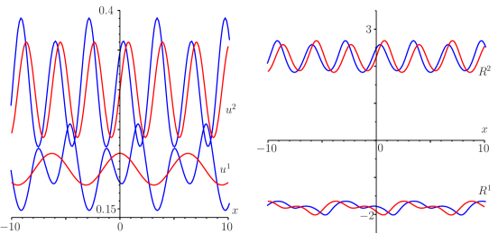
Figure 1: $a_{*}=-16.89$, $b_{*}=18.90$, $\delta\tau=0.5$, $x(a_{*},b_{*})=2.778$, $t(a_{*},b_{*})=8.982$

The second example demonstrates the Riemann problem solutions. We solve the general Riemann problem when the initial discontinuities is not piecewise constant.

$$u^{1}_{0}=(0.2-0.1h(x+2))(1+0.1\cos 2x),\quad 4\lambda=1,\quad\kappa=1$$ (2.55)

$$u^{2}_{0}=(0.3+0.1h(x-2))(1+0.1\sin 3x),$$

where $h(\tau)$ is the Heaviside step function.

On Fig. 2 the distribution of the densities at time $t=1.091$, $t=1.590$ are shown. The red lines correspond to the initial distribution.

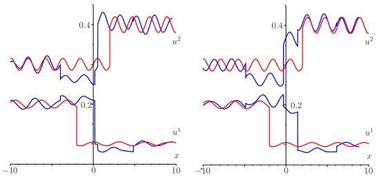
Figure 2: (left) $a_{*}=-2.89$, $b_{*}=0.90$, $\delta\tau=0.05$, $x(a_{*},b_{*})=-0.661$, $t(a_{*},b_{*})=1.091$; (right) $a_{*}=-4.89$, $b_{*}=0.90$, $\delta\tau=0.05$, $x(a_{*},b_{*})=-1.561$, $t(a_{*},b_{*})=1.590$

On Fig. 3 the distribution of the Riemann invariant at time $t=1.091$, $t=1.590$ are shown. The red lines correspond to the initial distribution.

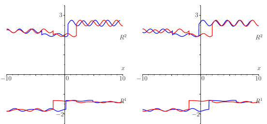
Figure 3: (left) $a_{*}=-2.89$, $b_{*}=0.90$, $\delta\tau=0.05$, $x(a_{*},b_{*})=-0.661$, $t(a_{*},b_{*})=1.091$; (right) $a_{*}=-4.89$, $b_{*}=0.90$, $\delta\tau=0.05$, $x(a_{*},b_{*})=-1.561$, $t(a_{*},b_{*})=1.590$

On Figs. 2, 3 the evolution of the discontinuities is well visible. As already mentioned, the simultaneous discontinuities of the invariants $R^{1}$, $R^{2}$ exist only at their the interaction. On the contrary, the discontinuities of the densities $u^{1}$, $u^{2}$ can be simultaneous.

III The shallow water equations

In this Section we present the numerical results for the shallow water equations omitted in previous paper Zhuk_Shir_ArXiv_2014_1 .

The classic version of the shallow water equations without taking into account the slope of the bottom has the form (see for example RozhdestvenskiiYanenko ; Whithem )

$$h_{t}+(hv)_{x}=0,\quad v_{t}+\left(\frac{1}{2}v^{2}+h\right)_{x}=0,$$ (3.1)

where $h>0$ is the elevation of the free surface, $v$ is the velocity.

We rewrite the equations in the form

$$u^{1}_{t}+(u^{1}u^{2})_{x}=0,\quad u^{2}_{t}+\left(\frac{1}{2}u^{2}u^{2}+u^{1}\right)_{x}=0,\quad h=u^{1},\quad v=u^{2}.$$ (3.2)

III.1 Interactions of the ‘solitons’

The initial distribution

$$u^{1}_{0}=1+0.2e^{-(x+3)^{2}}+0.2e^{-(x-3)^{2}},\quad u^{2}_{0}=0.2e^{-(x+3)^{2}}-0.2e^{-(x-3)^{2}}$$ (3.3)

simulates the interaction of two ‘solitons’. The initial perturbations of the free surface and velocity are given in the form of Gaussian distributions. The right perturbation moves to the left, and the left perturbation moves to the right.

The position of the free surface and the distribution of the velocity field for different moments of time are shown on Fig. 4–9.

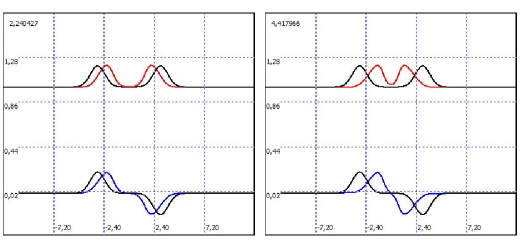
Figure 4: $h=u^{1}$ (red), $v=u^{2}$ (blue), the initial distributions (black)

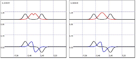
Figure 5: $h=u^{1}$ (red), $v=u^{2}$ (blue), the initial distributions (black)

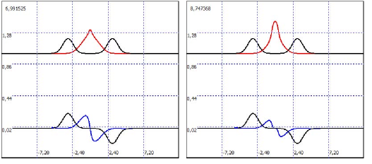
Figure 6: $h=u^{1}$ (red), $v=u^{2}$ (blue), the initial distributions (black)

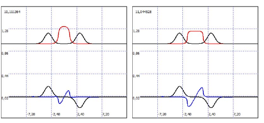
Figure 7: $h=u^{1}$ (red), $v=u^{2}$ (blue), the initial distributions (black)

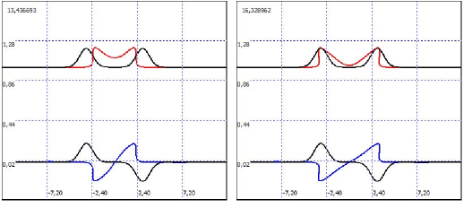
Figure 8: $h=u^{1}$ (red), $v=u^{2}$ (blue), the initial distributions (black)

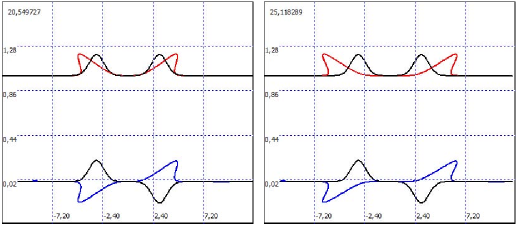
Figure 9: $h=u^{1}$ (red), $v=u^{2}$ (blue), the initial distributions (black)

III.2 Wave packet

We take the perturbation of the free surface in the wave packet form, assuming that the velocity is equal to nought

$$u^{1}_{0}=1.0+0.1\cos(3x)e^{x^{2}},\quad u^{2}_{0}=0.$$ (3.4)

The position of the free surface and the distribution of the velocity field for different moments of time are shown on Fig. 10, 11.

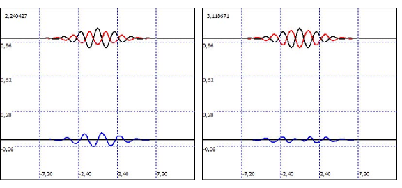
Figure 10: $h=u^{1}$ (red), $v=u^{2}$ (blue), the initial distributions (black)

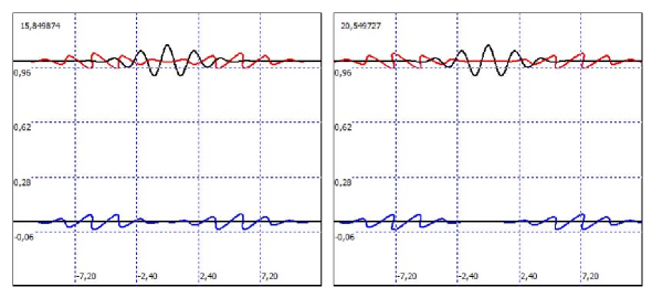
Figure 11: $h=u^{1}$ (red), $v=u^{2}$ (blue), the initial distributions (black)

IV Conclusions

The choice to study equations of two-beam reduction of the dense soliton gas is not random selection. First, these equations are degeneracy and, therefore, does not admit self-similar solutions. Secondly, the results of the Sec. II.4 show that the braking solution profile is impossible. All strong discontinuities are the so-called contact discontinuities, i.e. the discontinuities are moving along the characteristics. This, in particular, means that the proposed method allows to solve the Cauchy problem for arbitrary initial data, including discontinuous. Thirdly, the Riemann–Green function has a very simple form that allows us to easily analyze the solution and solve the Cauchy problem with initial data on an arbitrary curve. Note that the densities and fluxes of the conservation laws for equations of two-beam reduction of the dense soliton gas (as well as for equations of the zonal electrophoresis Zhuk_Shir_ArXiv_2014_2 ) can be constructed as linear combinations of the original conservation laws (see (2.9)–(2.14)). Unfortunately, we could not use this method in the case of the shallow water equations.

As already mentioned, the numerical method is accurate, as it does not require any approximations of the original problem. The most efficient method operates when there is an explicit expression for the Riemann–Green function. However, this method can be applied in cases when the Riemann–Green function is determined using the approximate solution of linear equations (A1.3)–(A1.7), for example, in the form of an infinite series or by using numerical methods. Of course, in this case, the inevitably there are errors associated with the construction of the Riemann–Green function.

We say a few words about the Cauchy problem (A1.18)–(A1.20). From our point of view, this problem is a generalization of the characteristics method to the case of two hyperbolic equations. Strictly speaking, formally, the method of characteristics for an arbitrary number of equations to construct is not very difficult. It is sufficient to consider the augmented system and construct the solution, for example, in the form of elementary waves RozhdestvenskiiYanenko ; Bressan . However, such equations are not closed. For the two equations the system can be closed, using the hodograph method and the Riemann–Green function. It would be interesting to build a similar scheme for solving the problem, bypassing the procedure to construct the Riemann–Green function of (and possibly hodograph method), at least for two hyperbolic quasilinear equations.

Appendix

Appendix A Reduction of the Cauchy problem for two
hyperbolic quasilinear PDE’s to the Cauchy problem for ODE’s

Referring for details to Zhuk_Shir_ArXiv_2014_1 ; Zhuk_Shir_ArXiv_2014_2 ; SenashovYakhno , here we give only a brief description of the method which allows to reduce the Cauchy problem for two hyperbolic quasilinear PDE’s to the Cauchy problem for ODE’s.

A.1 The Riemann invariants

Let for a system of two hyperbolic PDE’s, written in the Riemann invariants $R^{1}(x,t)$, $R^{2}(x,t)$, we have the Cauchy problem at $t=t_{0}$

$$R^{1}_{t}+\lambda^{1}(R^{1},R^{2})R^{1}_{x}=0,\quad R^{2}_{t}+\lambda^{2}(R^{1},R^{2})R^{2}_{x}=0,$$ (A1.1)

$$R^{1}(\tau,t_{0})=R^{1}_{0}(x),\quad R^{2}(x,t_{0})=R^{2}_{0}(x),$$ (A1.2)

where $R^{1}_{0}(x)$, $R^{2}_{0}(x)$ are the functions determined on some interval of the axis $x$ (possibly infinite), $\lambda^{1}(R^{1},R^{2})$, $\lambda^{2}(R^{1},R^{2})$ are the given functions.

We recall that any system of two quasilinear equations can be reduce to the Riemann invariants (see e.g. RozhdestvenskiiYanenko )

A.2 Hodograph method

Using the hodograph method for some conservation law $\varphi_{t}+\psi_{x}=0$, where $\varphi(R^{1},R^{2})$ is the density, $\psi(R^{1},R^{2})$ is the flux, we write the equation SenashovYakhno

$$\Phi_{R^{1}R^{2}}+A(R^{1},R^{2})\Phi_{R^{1}}+B(R^{1},R^{2})\Phi_{R^{2}}=0,$$ (A1.3)

$$A(R^{1},R^{2})=\frac{\lambda^{1}_{R^{2}}}{\lambda^{1}-\lambda^{2}},\quad B(R^{1},R^{2})=-\frac{\lambda^{2}_{R^{1}}}{\lambda^{1}-\lambda^{2}}.$$ (A1.4)

A.3 The Riemann–Green function

Let the function $\Phi(R^{1},R^{2}|r^{1},r^{2})$ is the Riemann–Green function for equation (A1.3). The function $\Phi(R^{1},R^{2}|r^{1},r^{2})$ of variables $R^{1}$, $R^{2}$ satisfies the given equation, and the function $\Phi(R^{1},R^{2}|r^{1},r^{2})$ of variables $r^{1}$, $r^{2}$ is the solution of the conjugate equation

$$\Phi_{r^{1}r^{2}}-(A(r^{1},r^{2})\Phi)_{r^{1}}-(B(r^{1},r^{2})\Phi)_{r^{2}}=0,$$ (A1.5)

with conditions

$$(\Phi_{r^{2}}-A\Phi)\bigr{|}_{r^{1}=R^{1}}=0,\quad(\Phi_{r^{1}}-B\Phi)\bigr{|}_{r^{2}=R^{2}}=0,$$ (A1.6)

$$\Phi\bigr{|}_{r^{1}=R^{1},r^{2}=R^{2}}=1.$$ (A1.7)

The methods of the Riemann–Green function construction are described, for example, in Copson ; Chirkunov ; Chirkunov_2 ; Courant ; Ibragimov ; SenashovYakhno .

A.4 Implicit solution of the problem

It is convenient, to write the density of a conservation law, i.e. the function $\varphi(R^{1},R^{2})$, in the form $\varphi(R^{1},R^{2}|r^{1},r^{2})$

$$\varphi(R^{1},R^{2}|r^{1},r^{2})=M(r^{1},r^{2})\Phi(R^{1},R^{2}|r^{1},r^{2}),\quad M(r^{1},r^{2})=\frac{2}{\lambda^{2}(r^{1},r^{2})-\lambda^{1}(r^{1},r^{2})}.$$ (A1.8)

The solution of (A1.1), (A1.2) can be represented in implicit form as SenashovYakhno

$$R^{1}(x,t)=r^{1}(b)=R^{1}_{0}(b),\quad R^{2}(x,t)=r^{2}(a)=R^{2}_{0}(a),$$ (A1.9)

where $a$, $b$ are the new variables (Lagrange variables).

The connection between the new variables $a$, $b$ and old variables $x$, $t$ has the form

$$t=t(a,b),\quad x=x(a,b).$$ (A1.10)

Function $t=t(a,b)$ is calculated using the density of the conservation law $\varphi(R^{1},R^{2}|r^{1},r^{2})$ and the initial data $R^{1}_{0}(x)$, $R^{2}_{0}(x)$ SenashovYakhno ; Zhuk_Shir_ArXiv_2014_1 ; Zhuk_Shir_ArXiv_2014_2

$$t(a,b)=t_{0}+\frac{1}{2}\int\limits_{a}^{b}\varphi(R^{1}_{0}(\tau),R^{2}_{0}(\tau)|r^{1}(b),r^{2}(a))\,d\tau.$$ (A1.11)

Function $x=x(a,b)$ is calculated by analogously SenashovYakhno , but this function is not required for further. We assume that this function is the given function.

If the equations (A1.10) are solvable explicitly

$$a=a(x,t),\quad b=b(x,t),$$ (A1.12)

then we have explicit solution

$$R^{1}(x,t)=R^{1}_{0}(b(x,t)),\quad R^{2}(x,t)=R^{2}_{0}(a(x,t)).$$ (A1.13)

A.5 Solution on isochrones

To construct the solution in the form (A1.9) in Zhuk_Shir_ArXiv_2014_1 we proposed to solve the Cauchy problem for ODE’s.

Fix some value $t=t_{*}$, specifying the level line (isochrone) of function $t(a,b)$

$$t_{*}=t(a,b).$$ (A1.14)

We assume that the isochrone is determined on the plane $(a,b)$ by the parametrical equations

$$a=a(\tau),\quad b=b(\tau),$$ (A1.15)

where $\tau$ is the parameter.

We choose the values $a_{*}$, $b_{*}$ which indicate some point on isochrone $t=t_{*}$

$$t_{*}=t(a_{*},b_{*}).$$ (A1.16)

In practice, the values of $a_{*}$, $b_{*}$ one can choose using the line levels of function $t(a,b)$ for some ranges of parameters $a$, $b$.

The coordinate $x$ on isochrone, obviously, is determined by the expression

$$x=x(a(\tau),b(\tau))\equiv X(\tau).$$ (A1.17)

To determine the $a(\tau)$, $b(\tau)$, $X(\tau)$ we have the Cauchy problem Zhuk_Shir_ArXiv_2014_1 ; Zhuk_Shir_ArXiv_2014_2

$$\frac{da}{d\tau}=-t_{b}(a,b),\quad\frac{db}{d\tau}=t_{a}(a,b),$$ (A1.18)

$$\frac{dX}{d\tau}=(\lambda^{2}(r^{1}(b),r^{2}(a))-\lambda^{1}(r^{1}(b),r^{2}(a)))t_{a}(a,b)t_{b}(a,b),$$ (A1.19)

$$a\bigr{|}_{\tau=0}=a_{*},\quad b\bigr{|}_{\tau=0}=b_{*},\quad X\bigr{|}_{\tau=0}=X_{*}.$$ (A1.20)

Here the values $a_{*}$, $b_{*}$ are given. To determine $X_{*}$ we need to solve the problem

$$\frac{dY(b)}{db}=x_{b}(a_{*},b)=\lambda^{2}(r^{1}(b),r^{2}(a_{*}))t_{b}(a_{*},b),\quad Y(a_{*})=a_{*}.$$ (A1.21)

Integrating from $a_{*}$ to $b_{*}$ we get

$$X_{*}=Y(b_{*}).$$ (A1.22)

Note, that $X_{*}=x(a_{*},b_{*})$ is the $x$ coordinate corresponding to $\tau=0$.

Solving (A1.18)–(A1.20) we obtain the solution on isochrone

$$R^{1}(x,t_{*})=R^{1}_{0}(b(\tau)),\quad R^{2}(x,t_{*})=R^{2}_{0}(a(\tau)),\quad x=X(\tau).$$ (A1.23)

Changing the parameter $\tau$ we obtain the solution which depends on $x$ as the fixed $t=t_{*}$. Pay attention to the fact that the right hand sides of differential equations, in particular, $t_{a}(a,b)$, $t_{b}(a,b)$ are easily computed with help of (A1.8), (A1.9), (A1.11).

Appendix B Additional simplification

Using another parameters $\theta$ instead $\tau$

$$d\tau={(R^{1}_{0}(a)-R^{2}_{0}(a))(R^{1}_{0}(b)-R^{2}_{0}(b))}d\theta$$ (B2.1)

one can simplify the equations (2.37), (2.38).

In this case instead of the equations (2.37), (2.38) we get

$$\frac{da}{d\theta}=R^{2}_{0}(a)-R^{1}_{0}(a),\quad\frac{db}{d\theta}=R^{2}_{0}(b)-R^{1}_{0}(b),\quad\frac{dX}{d\theta}=R^{2}_{0}(a)-R^{1}_{0}(b).$$ (B2.2)

References

- (1) Shiryaeva E. V., Zhukov M. Yu. Hodograph Method and Numerical Solution of the Two Hyperbolic Quasilinear Equations. Part I. Shallow water equations // (2014) arXiv:1410.2832. 19 p.
- (2) Shiryaeva E. V., Zhukov M. Yu. Hodograph Method and Numerical Solution of the Two Hyperbolic Quasilinear Equations. Part II. Zonal electrophoresis equations // (2015) arXiv:1503.01762. 23 p.
- (3) Senashov S. I., Yakhno A. Conservation laws, hodograph transformation and boundary value problems of plane plasticity // SIGMA. 2012. Vol. 8, 071. 16 p.
- (4) Rozdestvenskii B.L., Janenko N.N. Systems of Quasilinear Equations and Their Applications to Gas Dynamics [in Russian], Nauka, Moscow (1978); English transl.: Transl. Math. Monogr., Vol. 55, Amer. Math. Soc., Providence, R. I. (1983).
- (5) Whitham G. B. Linear and nonlinear wave. A Wiley-Interscience Publication John Willey & Sons, 1974, New-York–London–Sydney–Toronto.
- (6) El. G.A., Kamchatnov A.M. Kinetic equation for a dense soliton gas // ArXiv:nlin/0507016v2. 2006. 4 p.
- (7) Ferapontov E. V., Tsarev S. P. Systems of hydrodynamic type that arise in gas chromatography. Riemann invariants and exact solutions. (Russian) Mat. Model. 3 (1991), no. 2, 82–-91.
- (8) Kuznetsov N. N. Some mathematical questions of chromatography // Computation methohods and programming. 1967. No 6,242–258.
- (9) Elaeva M. S. Investigation of zonal elecrophoresis for two component mixture // (Russian) Mat. Model. 22 (2010), no. 9, 146–-160.
- (10) Elaeva M. S. Separation of two component mixture under action an electric field // Comp. Math. and Mat. Phys. 52:6 (2012), 1143–1159.
- (11) Babskii V. G., Zhukov M. Yu., Yudovich V. I. Mathematical Theory of Electrophoresis. Kluwer Academic / Plenum Publishers (1989).
- (12) Zhukov M. Yu. Non-staionary isotachophoresis model // Comp. Math. and Math. Phys. 1984. V. 24, No 4, 549–565. (in Rissian).
- (13) Zhukov M. Yu. Masstransport by an electric field. Rostov-on-Don: RGU Press, 2005. 215 p.
- (14) Copson E. T. On the Riemann-Green Function.Arch. Ration. Mech. Anal. 1 (1958) 324-348.
- (15) Courant R., Hilbert D. Methods of Mathematical Physics: Partial Differential Equations, Volume II. New York – London, 1964.
- (16) Ibragimov N. Kh. Group analysis of ordinary differential equations and the invariance principle in mathematical physics (for the 150th anniversary of Sophus Lie) // Russian Mathematical Surveys(1992),47(4):89. P. 83–144.
- (17) Chirkunov Yu. A. On the symmetry classification and conservation laws for quasilinear differential equations of second order // Mathematical Notes. 2010, Volume 87, Issue 1-2, pp 115-121.
- (18) Chirkunov Yu. A. Generalized equivalence transformations and group classification of systems of differential equations // Journal of Applied Mechanics and Technical Physics. 2012, Volume 53, Issue 2, pp 147-155.
- (19) O. F. Menshikh Conservation Laws of Second Order for the Born–Infeld Equation and Other Related Equations // Mat. Zametki, 84:6 (2008), 874–881.
- (20) Menshikh O. F. Conservation laws and Backlund transformations associated with the Born–Infeld equation // Mat. Zametki, 77:4 (2005), 551–565.
- (21) Menshikh O. F. Interaction of Born–Infeld solitons // Teoret. Mat. Fiz., 84:2 (1990), 181–194.
- (22) Menshikh O. F. Interaction of finite solitons for equations of Born–Infeld type // Teoret. Mat. Fiz., 79:1 (1989), 16–29.
- (23) Bressan A. Hyperbolic Conservation Laws. An Illustrated Tutorial // 2009, 81 p. http://www.math.psu.edu/bressan/PSPDF/clawtut09.pdf.