FORS2 observes a multi-epoch transmission spectrum of the hot Saturn-mass exoplanet WASP-49b^,

Abstract

Context. Transmission spectroscopy has proven to be a useful tool for the study of exoplanet atmospheres, because the absorption and scattering signatures of the atmosphere manifest themselves as variations in the planetary transit depth. Several planets have been studied with this technique, leading to the detection of a small number of elements and molecules (Na, K, $\mathrm{H_{2}O}$), but also revealing that many planets show flat transmission spectra consistent with the presence of opaque high-altitude clouds.

Aims. We apply this technique to the $M_{P}=0.40$ ${M}_{J}$, $R_{p}=1.20$ ${R}_{J}$, $P=2.78$ d planet WASP-49b, aiming to characterize its transmission spectrum between 0.73 and 1 $\muup$m and search for the features of K and $\mathrm{H_{2}O}$. Owing to its density and temperature, the planet is predicted to possess an extended atmosphere and is thus a good target for transmission spectroscopy.

Methods. Three transits of WASP-49b have been observed with the FORS2 instrument installed at the VLT/UT1 telescope at the ESO Paranal site. We used FORS2 in MXU mode with grism GRIS_600z, producing simultaneous multiwavelength transit light curves throughout the i’ and z’ bands. We combined these data with independent broadband photometry from the Euler and TRAPPIST telescopes to obtain a good measurement of the transit shape. Strong correlated noise structures are present in the FORS2 light curves, which are due to rotating flat-field structures that are introduced by inhomogeneities of the linear atmospheric dispersion corrector’s transparency. We accounted for these structures by constructing common noise models from the residuals of light curves bearing the same noise structures and used them together with simple parametric models to infer the transmission spectrum.

Results. We present three independent transmission spectra of WASP-49b between 0.73 and 1.02 $\muup$m, as well as a transmission spectrum between 0.65 and 1.02 $\muup$m from the combined analysis of FORS2 and broadband data. The results obtained from the three individual epochs agree well. The transmission spectrum of WASP-49b is best fit by atmospheric models containing a cloud deck at pressure levels of 1 mbar or lower.

1 Introduction

The study of transiting planets has become one of the main avenues for characterizing exoplanets. Transit light curves are observed while the planet passes between its host star and an Earth-based observer, and many pieces of information on the planetary system are contained in them. Most prominently, the planetary radius and, in conjunction with a mass estimate, the planetary density are measured. The atmospheric properties of transiting planets are accessible to study mainly through transmission and emission spectroscopy, that is, through multiwavelength observations of transits and occultations (for a summary, see, e.g., Winn 2011).

Transmission spectroscopy (e.g. Seager & Sasselov 2000, Charbonneau et al. 2002) is sensitive to the absorption features imprinted by the planetary atmosphere on the stellar light that passes through it during transit. In this configuration the planetary day-night terminator region is probed. The angle between the planetary surface and the incident stellar radiation causes the outer atmospheric layers to have a higher weight for these observations than for the emissive case.

On the observational side, a limitation to transmission spectroscopy is given by stellar activity. Non-occulted spots slightly affect the measured transit depth (e.g., McCullough et al. 2014). These effects are largely eliminated for inactive planet hosting stars and can be further decreased by carrying out simultaneous observations in the available wavelength channels. Spectrophotometry consists of spectrally dispersing the light of target and reference stars and then binning the spectra to a lower resolution and performing relative photometry on the summed stellar flux in these bins. In this way, simultaneous multiwavelength observations of transits can be obtained. Initial results stem from space-based observatories (Barman 2007, Knutson et al. 2007, Désert et al. 2008), but more recently, this technique has also been used in ground-based instruments where capabilities of obtaining spectra of multiple objects allow using comparison stars (Bean et al. 2010, 2011, Sing et al. 2011).

From high-resolution spectra, several absorption features, in particular that of Na (Charbonneau et al. 2002, Redfield et al. 2008), have been identified in the optical transmission spectra of giant planets. Initial near-IR detections based on HST/NICMOS data (e.g., Swain et al. 2008) have given rise to debate because independent analyses have yielded different results (Sing et al. 2009, Gibson et al. 2011, Crouzet et al. 2012). More recently, HST/WFC3 has been used on a few hot Jupiters, where absorption features of $\mathrm{H_{2}O}$ could be identified (e.g., Deming et al. 2013, Huitson et al. 2013). Compared to theoretical predictions (e.g., Seager & Sasselov 2000), these signatures have been less pronounced than expected, indicating that an additional, grayer, opacity source is present in the planetary atmospheres. This picture is supported by largely flat optical transmission spectra observed for several hot Jupiter planets (e.g., Pont et al. 2008, Bean et al. 2013, Gibson et al. 2013). If the slope of the transmission spectrum is measured across a broad wavelength region, the haze components can be revealed thanks to their Rayleigh scattering signature (e.g., Lecavelier Des Etangs et al. 2008).

The subject of this paper, WASP-49b, (Lendl et al. 2012) is a hot Saturn discovered by the WASP survey (Pollacco et al. 2006). WASP has been carrying out a search for hot Jupiters orbiting bright ($\mathrm{m_{V}<13}$) stars all across the sky. Lendl et al. (2012) measured a mass of 0.38 ${M}_{J}$ and a radius of 1.12 ${R}_{J}$ for WASP-49b, which is orbiting a G6 V star every 2.78 days. Given its low density (0.27 $\rho_{J}$) and short orbital period, the planet possesses an extended atmosphere and is thus a favorable target for transmission spectroscopy.

We here present transit observations of WASP-49b, obtained with the FORS2 instrument installed at the VLT/UT1. Observations of three transits of WASP-49b were obtained in multi-object spectroscopy (MXU) mode, covering wavelengths from 0.7 $\muup$m to 1.02 $\muup$m. These data are supplemented by additional transit observations from the EulerCam (Lendl et al. 2012) and TRAPPIST (Gillon et al. 2011b, Jehin et al. 2011) instruments. In Sect. 2, we report details of the observations and the data reduction, and in Sect. 3 we describe the modeling process. The resulting transmission spectrum is shown and interpreted in Sect. 4, before we conclude in Sect. 5.

2 Observations and data reduction

2.1 FORS2 spectrophotometry

2.1.1 Observations

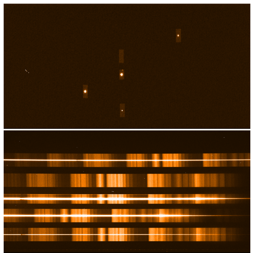
Figure 1: Top: An acquisition image for the WASP-49 FORS2 observations. The mask with five slits is visible, four of the slits are placed on stars, one is placed on the sky. Bottom: The same field and instrument setup, but with the dispersive element in the optical path.

Three transits of WASP-49b were observed with FORS2 (Appenzeller et al. 1998) at the VLT/UT1 during the nights of 05 December 2012, 14 January 2013 and 07 February 2013, under program 090.C-0758. The instrument was used in MXU mode, which allows performing ($R\sim 1000$) multi-object spectroscopy with the help of laser-cut masks made specifically for the observed field. We used wide 10 by 28 arcsec (in one case 10 by 20 arcsec) slits to select WASP-49 and three reference stars, and used grism GRIS_600z for the dispersion together with order sorting filter OG590. The large slit widths are needed to avoid flux losses during variations in seeing or pointing. The resulting wavelength range is $738-1026$ nm for WASP-49. The wavelength range of the reference stars is slightly different owing to their position on the detector and thus the displacement of the spectra on the chip. The positioning of the target and reference stars is shown in Fig. 1 and an example of the obtained spectra in Fig. 3. For the wavelength calibration we used a HeArNe lamp spectrum, but narrower (0.5 arcsec) slits were used to provide well-defined unsaturated emission lines to match with the database.

The linear atmospheric dispersion corrector (LADC) of FORS2 proved to impose a major limitation to the instrument’s photometric performance (Moehler et al. 2010) throughout several years until its upgrade in 2014 (Sedaghati et al. 2015). The data treated here fall into this period. The LADC is composed of two prisms whose separation is changed with airmass to compensate for the image dispersion caused by the atmosphere. These prisms show structures of uneven transmission. As the LADC is located in the optical path above the image derotator, this creates structures that rotate across the field of view during long observing sequences. To reduce noise stemming from the LADC, the LADC prism separation was set to a constant value throughout each of our transit observations. For the first two nights this value was set by the previous instrument configuration, that is, 155.0 mm for 05 December 2012, and 898.1 mm for 14 January 2013. As we observed that the long-term correlated noise in the photometry was reduced for the smaller prism separation, we set the LADC to a minimum separation of 30 mm for our third (14 February 2013) observation.

The weather during the first two transits was good, with stable seeing around 0.9 arcsec on 05 December 2012 and seeing varying between 0.8 and 1.5 arcsec on 14 January 2013. The data obtained on 07 February 2013 were affected by variable and partially unfavorable seeing, between 1.0 and 2.5 arcsec. The exposure times used were 30 s and 25 s for the first observation, and 20 s for the other observations. The third observation was interrupted by a technical malfunction before the beginning of the transit.

During the pre-imaging of the target field, we discovered a faint star ($\mathrm{\Delta mag_{z}=4.303\pm 0.12}$) located 2.3 arcsec south of WASP-49 (see Fig. 2). This star was blended with WASP-49 in previous observations.

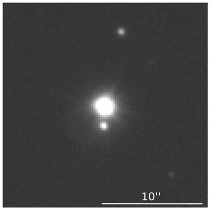
Figure 2: WASP-49b and the nearby star, as seen in the pre-imaging with FORS2. North is up and east is left.

2.1.2 Data reduction

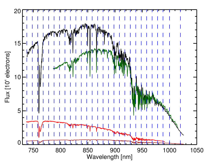
Figure 3: Example of the spectra of WASP-49 (top, black), and the three reference stars (green, red, brown). The blue dashed lines indicate the bin sizes used for spectrophotometry. Note that only two faint reference stars are available for the five shortest-wavelength bins.

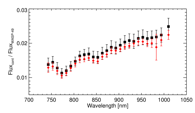
Figure 4: Relative flux of the nearby star contaminating the WASP-49 spectra, shown as a function of wavelength. The red diamonds show the contamination estimated from photometry after subtracting the target PSF, and black squares denote the results from comparison of the fitted PSF peaks. The slope of the measurements indicates an object redder than WASP-49.

The standard ESO pipeline was used to produce the master calibration frames, and to determine a wavelength solution in form of a third-order order polynomial based on the lamp frames. The wavelength solution was later refined by matching prominent absorption lines in the mean stellar spectra. To extract of spectrophotometric measurements, we proceeded as follows. For each pixel, the PSF in the spatial direction was determined iteratively by fitting Moffat functions (Moffat 1969) using the mpfit routines (Markwardt 2009). Outliers (mostly cosmic ray hits) were rejected at this step and then replaced by the values of the PSF fit at this point. The sky background was individually measured for each spectral pixel by fitting a first-order polynomial in the spatial direction selecting only regions well outside the stellar PSF. The sky contribution was then removed by subtracting this fit from all spatial pixels. By assuming a varying sky value for each spectral pixel, we compensated for slight variations in the background that are due to bends in the spectra with respect to the CCD pixel grid.

The 1D spectra were extracted for each spectral pixel, by summing the flux in several windows of different widths centered on the PSF peak. At this point, data affected by saturation of the detector during the 05 December 2012 observation were identified and removed from further analysis. To measure the amount of contamination introduced by the nearby star, we subtracted the stellar PSF from the 2D spectrum of WASP-49 and then measured the contaminant’s flux that fell inside each of the extraction windows. For a second estimate of the target to contaminant flux ratio, the PSF of the contaminant was fitted after the removal of the target PSF, and the peak values were compared. The resulting values averaged for all three transits and for each spectral bin are shown in Fig. 4. After we extracted the spectra of all exposures, we removed outliers once more, this time based on the temporal domain. For each spectral pixel, the extracted flux values were fit with a fourth-order polynomial with respect to time, outliers were identified and replaced by the values of the fit at the same position.

Next we binned the final spectra in 27 wavelength bins, 25 of which had a width of 10 nm, only the two longest-wavelength bins measured 12 nm and 20 nm. The location of these bins with respect to the spectra of target and reference stars is shown in Fig. 3. The five shortest-wavelength bins and the longest-wavelength bin are not covered by all reference stars. Relative photometric light curves were created for each extraction window from the binned spectra. All combinations of reference stars were tested; the best light curves were obtained using all references available in each wavelength bin.

For the further analysis, the light curves obtained from large extraction windows were used: 32 pixels for the transits on 05 December 2012 and 14 January 2013, and 36 pixels for the transit on 07 February 2013. This way, the contaminating star was contained in the aperture and its contribution to the light curve kept as stable as possible. The resulting light curves are displayed in Fig. 5.

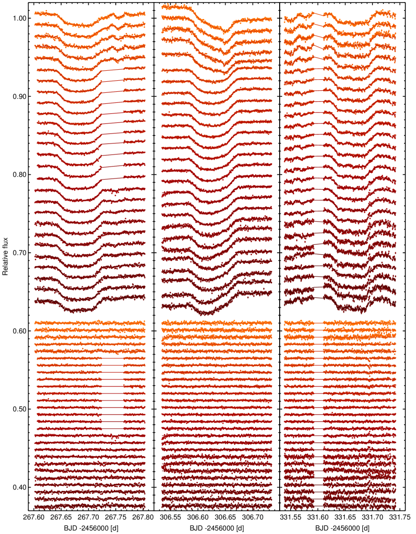
Figure 5: Spectro-photometric FORS2 transit light curves of WASP-49. The wavelength of the individual light curves increases downward, and the bin centers are 743, 753, 763, 773, 783, 793, 803, 813, 823, 833, 843, 853, 863, 873, 883, 893, 903, 913, 923, 933, 943, 953, 963, 973, 983, 994, and 1010 nm. The residuals are shown below the data.

2.1.3 FORS2 data of 05 December 2012

The FORS2 observations of 5 December 2012 were carried out throughout the transit using an exposure time of 30 s. The peak region of the target spectrum exceeded the nonlinear range of the detector from $\sim$05:15 UT on, until the exposure time was adapted down to 25 s at 06:14 UT. Points affected by this episode of saturation were identified during the spectral extraction and removed from further analysis.

The $\lambda<788$ nm light curves show a very particular wave-like pattern around meridian passage. These are the same light curves that were created using only two reference stars. This effect arises because the spatial inhomogeneities of the LADC transparency creates differences in the light curves of the comparison stars.

2.1.4 FORS2 data of 14 January 2013

Again, the $\lambda<788$ nm light curves obtained with FORS2 on 14 January 2013 show a wave-like pattern around meridian passage, probably for the same reason as for the 5 December 2012 data. At the same time, the overall light curve shapes are more strongly affected, with large-scale tilts that vary in shape and amplitude. This is probably related to the fact that the LADC separation was large for this observation, 898.1 mm as opposed to 155.0 mm for the 05 December 2012 observation.

2.1.5 FORS2 data of 07 February 2013

The FORS2 data taken on 7 February 2013 were affected by less favorable conditions, than the other transit observations, in particular, by bad seeing. The observations were interrupted because of a technical problem at 02:08 UT, but were resumed at 02:29 UT, ~20 minutes before the start of the transit. The data obtained before the interruption show large variations, related to unfavorable observing conditions and the passage of meridian and hence fast LADC movement. Some light curves show an unexplained short-term increase in flux during egress, which probably is of instrumental origin.

2.2 EulerCam and TRAPPIST photometry

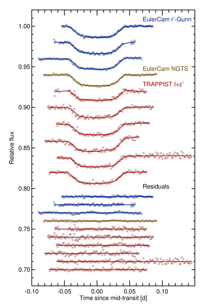
Figure 6: WASP-49 transit light curves from EulerCam and TRAPPIST included in the analysis. The instrument and filters are color coded and are (from top to bottom) EulerCam using an r’-Gunn filter (top three), EulerCam using the NGTS filter (fourth), and TRAPPIST using an I+z’ filter (all remaining light curves). The TRAPPIST data are binned in two-minute intervals.

Two additional transit light curves of WASP-49 were obtained using EulerCam at the 1.2 m Euler-Swiss telescope at the La Silla site (Chile). During the night of 5 December 2012 we observed through a wide (520 nm to 880 nm) filter designed for the upcoming NGTS survey (Wheatley et al. 2013), while during the night of 30 December 2012, an r’-Gunn filter was used. The telescope was slightly defocused for both observations, and exposure times were between 35s and 60s (December 5), and 90s (December 30). The data were reduced using relative aperture photometry. More details on instrument and reduction can be found in Lendl et al. (2012).

The TRAnsiting Planets and PlanetesImals Small Telescope (TRAPPIST, Gillon et al. 2011b, Jehin et al. 2011) is also located at the La Silla site. It was used to observe four more transits through an I+z’ filter during the nights of 5, 16, and 30 December 2012, and 21 February 2013. The exposure times used were 6 s (first two transits) and 10 s (last two transits). The light curves were produced using relative aperture photometry, where several apertures were tested and the ideal combination of reference stars was found. IRAF was used in the reduction process.

We also included in the analysis the two full transit light curves of each EulerCam and TRAPPIST that have been already described in Lendl et al. (2012). All broadband light curves are shown in Figure 6.

3 Modeling

3.1 Method

To derive the transmission spectrum of the planet and find improved measurements of the planetary and stellar parameters, a Markov chain Monte Carlo (MCMC) approach was used. Included in the analysis were all available photometric data as described in Sect. 2 (FORS2, EulerCam, and TRAPPIST).

We made use of a modified version of the adaptive MCMC code described in detail in Gillon, M. et al. (2012). In this code, the prescription of Mandel & Agol (2002) is used to model the transit light curves. To compensate for correlated noise in the light curves, parametrizations of external variables (such as time, stellar FWHM, and coordinate shifts) can be included in the photometric baselines models. These models typically consist of polynomials up to fourth order that are multiplied with the theoretical transit light curve. Their coefficients are found by least-squares minimization at every MCMC step.

3.1.1 Common noise model

In this updated version of the code, it is possible to also include a common noise model (CNM) for a set of light curves carrying the same correlated noise structure. This CNM is created at each MCMC step by fitting a model transit light curve based on the current parameter state together with an invariable, previously determined, normal distribution for the transit depth with a center $dF_{group}$, and then co-adding the residuals of this fit. For each time step $t_{i}$, the CNM is calculated as

$$CNM_{i}=\sum_{k=0}^{n_{lc}}\left(\frac{O_{i,k}}{C_{i,k}}\,w^{-1}_{i,k}\right)\,,$$ (1)

where $n_{lc}$ is the total number of light curves the CNM is calculated for, $O_{i}$ are the observed data, and $C_{i}$ are the transit model values. Weights $w_{i,k}$ are attributed according to measurement errors $err_{i,k}$,

$$w_{i,k}=err^{2}_{i,k}\,{\sum_{k=0}^{n_{lc}}\frac{1}{err_{i,k}^{2}}}\,.$$ (2)

See Fig. 7 for an example of a CNM obtained from FORS2 data. This approach is similar to the use of the white light curves for the definition of the correlated noise component by Stevenson et al. (2014) and others.

Figure 7: Example of a CNM, calculated as described in Sect. 3.1.1. Here, the CNM of the $\lambda<788$ nm data of 05 December 2012 is shown.

3.1.2 Fitted and fixed parameters

In the analysis of our combined photometric dataset, the following variables were MCMC fitted (”jump“) parameters:

• The impact parameter $b^{\prime}=a\cos(i_{p})/R_{\ast}$, where $R_{\ast}$ denotes the stellar radius, $a$ the semi-major axis of the planetary orbit, and $i_{p}$ the orbital inclination.

• The transit duration $T_{14}$

• The time of mid-transit $T_{0}$

• The orbital period $P$

• The stellar parameters effective temperature $T_{eff}$ and metallicity [Fe/H].

• If desired (as for the test in Sect. 3.2.4), the linear combination of the quadratic limb-darkening coefficients $(u_{1},u_{2})$ in each wavelength band, $c_{1,i}=2u_{1,i}+u_{2,i}$ and $c_{2,i}=u_{1,i}-2u_{2,i}$ (Holman et al. 2006).

• If a single value of the transit depth is desired (step 1 in our analysis), $dF_{0}=(R_{p}/R_{\ast})^{2}$ is included as a jump parameter.

• If a transmission spectrum is fit (i.e. several values of $dF$, step 2 in our analysis), offsets $ddF_{i}$ to a pre-defined value for $dF_{0}$.

• If a CNM is included, an a priori estimate of the transit depth of each group, $dF_{group}$.

The value for the RV amplitude was set to that of the discovery paper. The eccentricity was set to zero as there has been no evidence for an eccentric orbit of WASP-49b. A quadratic model of the form $I(\mu)=I_{\mathit{center}}\left(1-u_{1}\left(1-\mu\right)-u_{2}\left(1-\mu\right)^{2}\right)$ (where $\mu=\cos{\theta}$ and $\theta$ is the angle between the surface normal of the star and the line of sight) was used to account for the effect of stellar limb-darkening on the transit light curves. The coefficients $u_{1}$ and $u_{2}$ were found by interpolating the tables of Claret & Bloemen (2011) to match the wavelength bands of our observations. The limb-darkening parameters were kept fixed to the values given in Table 1 throughout our analysis, but we verified our results by allowing for variable limb-darkening coefficients as described in Sect. 3.2.4.

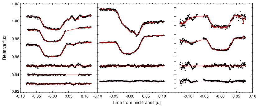
Figure 8: FORS2 spectrophotometry and residuals obtained from using a single bin for each light curve subset, as described in Sect. 3.2.1. The three subsets of 05 December 2012 are shown in the left panel and correspond to wavelength ranges of (from top to bottom) 738-788, 788-898, and 898-1020 nm. The middle and right panels show the two subsets of 14 January 2013 and 07 February 2013, respectively, and correspond to wavelength ranges of (from top to bottom) 738-788, and 788-1020 nm. The models are shown as red solid lines and contain the parametrizations of external parameters as described in Table 2. The residuals are shown below the data which are partially offset for clarity.

Table 1: Limb-darkening coefficients used in the analysis of the photometric data.

Wavelength [nm]	$u_{1}$	$u_{2}$
738 - 748	$0.318$	$0.275$
748 - 758	$0.315$	$0.273$
758 - 768	$0.311$	$0.272$
768 - 778	$0.309$	$0.27$
778 - 788	$0.306$	$0.268$
788 - 798	$0.303$	$0.267$
798 - 808	$0.3$	$0.265$
808 - 818	$0.298$	$0.264$
818 - 828	$0.295$	$0.262$
828 - 838	$0.292$	$0.261$
838 - 848	$0.289$	$0.26$
848 - 858	$0.286$	$0.259$
858 - 868	$0.282$	$0.258$
868 - 878	$0.279$	$0.258$
878 - 888	$0.275$	$0.257$
888 - 898	$0.27$	$0.258$
898 - 908	$0.265$	$0.258$
908 - 918	$0.259$	$0.259$
918 - 928	$0.253$	$0.26$
928 - 938	$0.247$	$0.261$
938 - 948	$0.239$	$0.263$
948 - 958	$0.231$	$0.266$
958 - 968	$0.222$	$0.269$
968 - 978	$0.213$	$0.272$
978 - 988	$0.202$	$0.276$
988 - 1000	$0.189$	$0.281$
1000 - 1020	$0.169$	$0.29$
r’	$0.28$	$0.26$
NGTS	$0.34$	$0.28$
I+z’	$0.29$	$0.26$

Uniform prior distributions were assumed for most parameters, but for the stellar effective temperature $T_{eff}$ and metallicity [Fe/H], normal prior distributions were used. These priors were centered on the values of Lendl et al. (2012) and their widths were defined as the 1- $\sigma$ errors of these values. If transmission spectra were derived, a normal prior was applied to $dF_{0}$, with a width of the 1- $\sigma$ errors of the used input value. We used the method described in Enoch et al. (2010) and Gillon et al. (2011a) to derive the stellar radius and mass from the transit light curve, stellar temperature and metallicity. The contribution (and its error) from the neighboring star was included in the analysis and the transit depths were adapted. At each instance, two MCMC chains were run and convergence of the MCMC chains was checked for all results with the Gelman & Rubin test (Gelman & Rubin 1992).

3.1.3 Photometric error adaptation

The photometric error bars were rescaled by calculating the white $\beta_{w}$ and red $\beta_{r}$ noise scale factors. $\beta_{w}$ is given by the ratio of the mean photometric error and the standard deviation of the final photometric residuals, and $\beta_{r}$ (Winn et al. 2008, Gillon et al. 2010) is derived by comparing the standard deviations of the binned and unbinned residuals. We multiplied our errors with their product $CF=\beta_{r}\times\beta_{w}$ derived from an initial MCMC run of $10^{4}$ points. The CF values are given in Table 3.2.4.

3.1.4 Baseline models for the FORS2 data

The FORS2 data are affected by the rotation of the LADC with respect to the detector and therefore show a strong noise component correlated with the parallactic angle. For these light curves, we tested baseline models involving the parallactic angle $\mathit{par}$, the change in parallactic angle $\mathit{dpar}$ (i.e., the derotator speed), and the trigonometric functions $\sin(\mathit{par})$ and $\cos(\mathit{par})$. Including the parallactic angle in baseline models for the FORS2 data leads to a much better fit of the overall light curve shapes than time-dependent models. Similarly, including the CNM in the photometric baseline produces very good fits to the data, efficiently accounting for short-term photometric variations that consistently appear in sets of light curves, but cannot be modeled as simple dependencies on external parameters.

3.2 Step-by-step procedure

We carried out the analysis with the aim to first infer the most reliable analysis method for the FORS2 data, and then applied it to obtain an accurate transmission spectrum for WASP-49b. To do so, we proceeded in the steps outlined below.

3.2.1 Step 1: An overall transit depth

We first identified the light curves that are affected by the same photometric variations and hence should form the subsets possessing the same CNM. For all three dates, a clear division is seen between the light curves obtained with two reference stars (the five shortest-wavelength bins, as well as the light curve centered on the K feature), and all other light curves. This is a clear consequence of the LADC being at the root of the strongest correlated noise source, as spatially varying transmission affects each reference star differently. For the data of 05 December 2012, we further subdivided the remaining light curves into two groups, light curves between 788 and 898 nm, which have fewer points because of detector saturation, and the light curves at wavelengths above 898 nm, where counts remained in the linear detector range.

For each subset, we combined all data to produce a “white” light curve. We then tested a number of photometric baseline models for these white light curves, finding the best modeling of these curves by accounting for large trends by means of second-order polynomials in $\mathit{par}$ and modeling the short-timescale variations in the $\lambda<788$ nm light curves using fourth-order polynomials in $\cos(par)$ or $\mathit{dpar}$, or a first-order polynomial in the stellar FWHM. These baseline functions are listed in Table 2. For the 05 December 2012 data, an offset is included at the change of exposure time. We then performed a combined MCMC analysis on all white light curves, allowing for a single transit depth. The result obtained is our best absolute transit depth $dF_{0}$, which was then used to calculate the transmission spectrum. These light curves are shown in Fig. 8. We find a resulting value for the transit depth of $dF_{0}=0.0133\pm 0.0002$.

Table 2: Baseline functions used in step 1 of our analysis, where a single transit depth is inferred from the binned data of all light curve subsets. The baseline functions of the form $p^{j}(i)$ denote a polynomial of order $j$ in parameter $i$, where $i$ can be the parallactic angle $par$, its cosine $\cos(par)$, the differential parallactic angle from one exposure to the next $\mathit{dpar}$, and the PSF or spectral full-width at half maximum $\mathit{fwhm}$. $\mathit{off}$ refers to an offset included at the change in exposure time for the 05 December 2012 observations.

Wavelength [nm]	Date	Baseline function
738 - 788	05 Dec 2012	$p^{4}(\cos(\mathit{par}))+\mathit{off}$
788 - 898	05 Dec 2012	$p^{2}(\mathit{par})+\mathit{off}$
898 - 1020	05 Dec 2012	$p^{2}(\mathit{par})+\mathit{off}$
738 - 788	14 Jan 2013	$p^{2}(\mathit{par})+p^{4}(\mathit{dpar})$
738 - 1020	14 Jan 2013	$p^{2}(\mathit{par})$
738 - 788	07 Feb 2013	$p^{1}(\mathit{fwhm})+p^{2}(\mathit{par})$
738 - 1020	07 Feb 2012	$p^{1}(\mathit{fwhm})+p^{2}(\mathit{par})$

3.2.2 Step 2: Individual transmission spectra

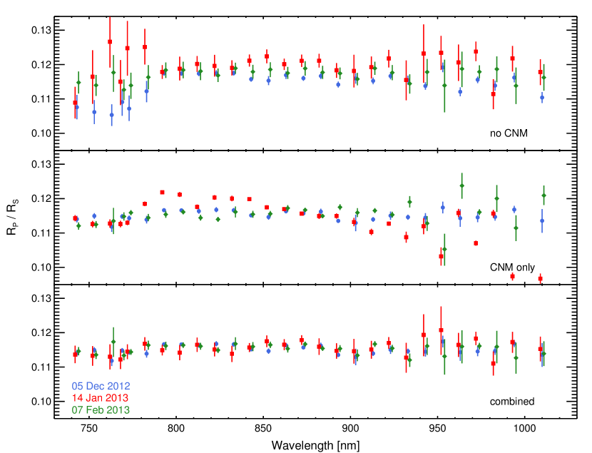
Figure 9: FORS2 transmission spectra of the three dates obtained with three baseline modeling approaches: no CNM, but parametrizations of external parameters as given in Sect. 9 (top), CNM alone (middle), and CNM together with basic parametrizations as detailed in Sect. 9 (bottom). Blue filled circles denote the FORS2 transmission spectrum of 05 December 2012, red squares that of 14 January 2013, and green diamonds that of 07 February 2013. In this plot, the spectra of 14 January 2013 and 07 February 2013 are offset from their nominal wavelengths by 1 nm to avoid overlaps.

We then derived individual transmission spectra for each date. Keeping an a priory transit depth fixed to the previously obtained $dF_{0}$, we inferred offsets $ddF_{i}$ from this value for each light curve. At this point, we searched for the best baseline models for each previously defined light curve set, testing three approaches, that relied to various degrees on the CNM.

1. No CNM: the photometric baselines consist solely of functions of external parameters, that is, $par$, $\cos(\mathit{par})$, $\mathit{dpar}$, and $\mathit{FWHM}$. These functions, and the wavelength range for light curves to which they are applied, are the same as inferred in Sect. 3.2.1 and listed in Table 2.

2. CNM only: no parametrizations of external variables are used, except for the offset at the exposure time change for the 05 December 2012 data. All light curves are fit with a first-order polynomial of the CNM (i.e., a function of the form $a_{0}+a_{1}\,\mathit{CNM}$) only. As mentioned in Sect. 3.1.1, the CNMs are calculated based on an input distribution for the transit depth. We used a Gaussian centered on the previously obtained $dF_{0}$, with a width of the 1-$\sigma$ error bars on $dF_{0}$. Higher-order polynomials with respect to the CNM were tested but did not improve the results.

3. Combined: the photometric baseline functions include the CNM and low-order polynomials of external parameters. The best baseline models were found to consist of first-order polynomials of the CNM, together with second-order polynomials of $\mathit{par}$ (January and February data).

The resulting transmission spectra are shown in Fig. 9: the results obtained without CNM (top panel) show larger error bars than the other modeling approaches, while the data are noisier at low wavelengths and show overall offsets between the three dates, most remarkably a median offset of 0.005 in $R_{p}/R_{\ast}$ between the data of 06 December 2012 and 14 January 2013. The transmission spectra inferred from CNM-only models (middle panel) have greatly reduced error bars, but the spectra inferred from the three dates do not agree, with substantial scatter at long wavelengths. The 14 January 2013 data show a distinct slope between 790 and 900 nm, a structure not reproduced for the other dates. The best agreement between the spectra from the three dates is found if the CNM and low-order parametrizations of external parameters are used together (third panel), and we used this approach to derive of our final transmission spectrum.

3.2.3 Step 3: A combined transmission spectrum

The final transmission spectrum was inferred from a global analysis of all available photometric data: the three FORS2 observations, and all available additional EulerCam and TRAPPIST broadband photometry. As the latter are light curves obtained with different instruments at different dates, CNMs cannot be applied to these data. The light curves are displayed in Fig. 6 (broadband), and Fig. 5, and the respective baseline functions are given in Table 3.2.4. For the analysis of the FORS2 data, we chose the third option outlined above: using CNMs together with functions of $par$ (and an offset at the change of exposure time in the 5 December 2012 data). The light curve subsets contributing to each CNM are the seven subsets defined above (three for the 5 December 2012 data, and two each for the 14 January 2013 and 7 February 2013 data). The analysis consisted of two MCMC chains of $10^{5}$ points each, allowing only for unique values of the transit depths for each wavelength bin. The resulting transmission spectrum is shown in Fig. 11.

3.2.4 Stellar limb-darkening

As stellar limb-darkening affects the transit shape, we decided to verify our transmission spectrum against variation in the limb-darkening coefficients. To do so, we carried out additional global analyses (identical to those described in Sect. 3.2.3), while allowing the limb-darkening coefficients to vary, assuming a normal prior distribution for them. This prior was centered on the interpolated value and had a width large enough to encompass the values of the neighboring passbands at 1-$\sigma$. The results are consistent with our previously derived transmission spectrum: when a prior is included, the maximum offset between the two runs is $0.14\sigma$ and the transmission spectra uncertainties are similar. longtablelllllll Details on the observations: wavelength band, date, baseline parameters and noise statistics of all data included in the global analysis of WASP-49b. The baseline functions of the form $p^{j}(i)$ denote a polynomial of order $j$ in parameter $i$, where $i$ can be time $t$, parallactic angle $\mathit{par}$, the sky background $\mathit{sky}$ and the PSF or spectral full-width at half maximum $\mathit{fwhm}$. $\mathit{off}$ refers to an offset due to the change in exposure time on FORS2, or a telescope meridian flip for some TRAPPIST light curves. The red- and white noise amplitudes $\beta_{r}$ and $\beta_{w}$, the error adaptation factor $\mathit{CF}$, and the RMS is given for data binned in bins of two minutes. For the FORS2 data, the four data quality parameters are given for the global fit (left value) and for fits restricted to single transit events (right value).
Wavelength [nm] Date Baseline function   $\beta_{r}$   $\beta_{w}$   CF $\mathrm{RMS_{120s}}$ [%]
FORS2
738 - 748 05 Dec 2012 $p^{1}(\mathit{CNM})+\mathit{off}$ $1.33$  $1.33$ $0.97$  $0.97$ $1.29$  $1.29$ $0.080$  $0.081$
14 Jan 2013 $p^{1}(\mathit{CNM})+p^{2}(\mathit{par})$ $1.12$  $1.15$ $1.00$  $0.99$ $1.12$  $1.14$ $0.074$  $0.087$
07 Feb 2013 $p^{1}(\mathit{CNM})+p^{2}(\mathit{par})$ $1.98$  $1.18$ $0.88$  $0.90$ $1.74$  $1.06$ $0.081$  $0.093$
748 - 758 05 Dec 2012 $p^{1}(\mathit{CNM})+\mathit{off}$ $1.24$  $1.13$ $0.81$  $0.99$ $1.01$  $1.12$ $0.055$  $0.074$
14 Jan 2013 $p^{1}(\mathit{CNM})+p^{2}(\mathit{par})$ $1.58$  $1.27$ $1.11$  $0.97$ $1.75$  $1.23$ $0.083$  $0.088$
07 Feb 2013 $p^{1}(\mathit{CNM})+p^{2}(\mathit{par})$ $1.50$  $1.20$ $0.52$  $0.87$ $0.77$  $1.04$ $0.022$  $0.083$
758 - 768 05 Dec 2012 $p^{1}(\mathit{CNM})+\mathit{off}$ $1.39$  $2.01$ $0.70$  $0.86$ $0.98$  $1.74$ $0.044$  $0.082$
14 Jan 2013 $p^{1}(\mathit{CNM})+p^{2}(\mathit{par})$ $1.02$  $1.50$ $0.71$  $0.92$ $0.73$  $1.37$ $0.045$  $0.093$
07 Feb 2013 $p^{1}(\mathit{CNM})+p^{2}(\mathit{par})$ $1.03$  $3.71$ $0.71$  $0.91$ $0.73$  $3.36$ $0.045$  $0.122$
768 - 778 05 Dec 2012 $p^{1}(\mathit{CNM})+\mathit{off}$ $1.48$  $1.25$ $0.69$  $0.81$ $1.02$  $1.01$ $0.044$  $0.054$
14 Jan 2013 $p^{1}(\mathit{CNM})+p^{2}(\mathit{par})$ $1.49$  $1.18$ $0.66$  $0.82$ $0.98$  $0.97$ $0.043$  $0.064$
07 Feb 2013 $p^{1}(\mathit{CNM})+p^{2}(\mathit{par})$ $1.31$  $1.00$ $0.72$  $0.76$ $0.95$  $0.76$ $0.045$  $0.058$
778 - 788 05 Dec 2012 $p^{1}(\mathit{CNM})+\mathit{off}$ $1.00$  $1.57$ $0.68$  $1.11$ $0.68$  $1.75$ $0.042$  $0.081$
14 Jan 2013 $p^{1}(\mathit{CNM})+p^{2}(\mathit{par})$ $1.41$  $1.09$ $0.72$  $0.93$ $1.02$  $1.01$ $0.052$  $0.070$
07 Feb 2013 $p^{1}(\mathit{CNM})+p^{2}(\mathit{par})$ $0.97$  $1.49$ $0.77$  $0.87$ $0.80$  $1.29$ $0.047$  $0.078$
765 - 773 (K) 05 Dec 2012 $p^{1}(\mathit{CNM})+\mathit{off}$ $3.68$  $1.42$ $1.07$  $0.69$ $3.94$  $0.98$ $0.077$  $0.044$
14 Jan 2013 $p^{1}(\mathit{CNM})+p^{2}(\mathit{par})$ $1.39$  $1.50$ $0.81$  $0.76$ $1.13$  $1.15$ $0.047$  $0.068$
07 Feb 2013 $p^{1}(\mathit{CNM})+p^{2}(\mathit{par})$ $2.51$  $1.57$ $0.80$  $0.73$ $2.01$  $1.14$ $0.056$  $0.078$
788 - 798 05 Dec 2012 $p^{1}(\mathit{CNM})+\mathit{off}$ $1.09$  $1.02$ $1.03$  $0.72$ $1.12$  $0.73$ $0.063$  $0.046$
14 Jan 2013 $p^{1}(\mathit{CNM})+p^{2}(\mathit{par})$ $1.87$  $1.10$ $1.05$  $0.82$ $1.96$  $0.91$ $0.085$  $0.051$
07 Feb 2013 $p^{1}(\mathit{CNM})+p^{2}(\mathit{par})$ $2.50$  $1.71$ $1.01$  $0.78$ $2.53$  $1.34$ $0.085$  $0.064$
798 - 808 05 Dec 2012 $p^{1}(\mathit{CNM})+\mathit{off}$ $3.50$  $1.04$ $1.03$  $0.70$ $3.61$  $0.73$ $0.097$  $0.045$
14 Jan 2013 $p^{1}(\mathit{CNM})+p^{2}(\mathit{par})$ $2.00$  $1.69$ $0.96$  $0.76$ $1.93$  $1.29$ $0.078$  $0.047$
07 Feb 2013 $p^{1}(\mathit{CNM})+p^{2}(\mathit{par})$ $1.53$  $1.19$ $0.99$  $0.73$ $1.52$  $0.87$ $0.080$  $0.056$
808 - 818 05 Dec 2012 $p^{1}(\mathit{CNM})+\mathit{off}$ $1.39$  $1.48$ $1.04$  $0.69$ $1.45$  $1.02$ $0.080$  $0.044$
14 Jan 2013 $p^{1}(\mathit{CNM})+p^{2}(\mathit{par})$ $3.72$  $1.54$ $1.20$  $0.76$ $4.46$  $1.18$ $0.116$  $0.048$
07 Feb 2013 $p^{1}(\mathit{CNM})+p^{2}(\mathit{par})$ $1.14$  $1.45$ $1.00$  $0.74$ $1.14$  $1.08$ $0.088$  $0.061$
818 - 828 05 Dec 2012 $p^{1}(\mathit{CNM})+\mathit{off}$ $1.27$  $1.47$ $0.97$  $0.66$ $1.23$  $0.98$ $0.088$  $0.043$
14 Jan 2013 $p^{1}(\mathit{CNM})+p^{2}(\mathit{par})$ $1.49$  $1.48$ $0.92$  $0.79$ $1.37$  $1.17$ $0.092$  $0.053$
07 Feb 2013 $p^{1}(\mathit{CNM})+p^{2}(\mathit{par})$ $1.18$  $1.27$ $0.82$  $0.70$ $0.97$  $0.90$ $0.064$  $0.051$
828 - 838 05 Dec 2012 $p^{1}(\mathit{CNM})+\mathit{off}$ $1.09$  $1.29$ $0.93$  $0.73$ $1.01$  $0.94$ $0.070$  $0.046$
14 Jan 2013 $p^{1}(\mathit{CNM})+p^{2}(\mathit{par})$ $1.47$  $1.63$ $0.66$  $0.85$ $0.97$  $1.38$ $0.055$  $0.053$
07 Feb 2013 $p^{1}(\mathit{CNM})+p^{2}(\mathit{par})$ $1.50$  $2.75$ $0.77$  $0.78$ $1.15$  $2.13$ $0.068$  $0.065$
838 - 848 05 Dec 2012 $p^{1}(\mathit{CNM})+\mathit{off}$ $1.11$  $1.00$ $0.82$  $0.68$ $0.91$  $0.68$ $0.052$  $0.042$
14 Jan 2013 $p^{1}(\mathit{CNM})+p^{2}(\mathit{par})$ $1.69$  $1.05$ $0.77$  $0.72$ $1.29$  $0.76$ $0.048$  $0.038$
07 Feb 2013 $p^{1}(\mathit{CNM})+p^{2}(\mathit{par})$ $1.56$  $1.90$ $0.76$  $0.73$ $1.18$  $1.38$ $0.048$  $0.058$
848 - 858 05 Dec 2012 $p^{1}(\mathit{CNM})+\mathit{off}$ $1.48$  $1.43$ $0.79$  $0.71$ $1.17$  $1.02$ $0.053$  $0.052$
14 Jan 2013 $p^{1}(\mathit{CNM})+p^{2}(\mathit{par})$ $1.63$  $1.29$ $0.85$  $0.78$ $1.38$  $1.00$ $0.054$  $0.047$
07 Feb 2013 $p^{1}(\mathit{CNM})+p^{2}(\mathit{par})$ $1.05$  $1.57$ $0.72$  $0.68$ $0.76$  $1.07$ $0.038$  $0.051$
858 - 868 05 Dec 2012 $p^{1}(\mathit{CNM})+\mathit{off}$ $1.28$  $1.06$ $0.78$  $0.76$ $1.00$  $0.80$ $0.047$  $0.046$
14 Jan 2013 $p^{1}(\mathit{CNM})+p^{2}(\mathit{par})$ $1.26$  $1.25$ $0.74$  $0.74$ $0.93$  $0.93$ $0.046$  $0.046$
07 Feb 2013 $p^{1}(\mathit{CNM})+p^{2}(\mathit{par})$ $1.06$  $1.83$ $0.77$  $0.64$ $0.81$  $1.17$ $0.045$  $0.051$
868 - 878 05 Dec 2012 $p^{1}(\mathit{CNM})+\mathit{off}$ $1.80$  $1.05$ $0.80$  $0.72$ $1.44$  $0.75$ $0.048$  $0.047$
14 Jan 2013 $p^{1}(\mathit{CNM})+p^{2}(\mathit{par})$ $1.54$  $1.06$ $0.84$  $0.77$ $1.29$  $0.81$ $0.056$  $0.045$
07 Feb 2013 $p^{1}(\mathit{CNM})+p^{2}(\mathit{par})$ $2.02$  $1.22$ $0.98$  $0.66$ $1.98$  $0.81$ $0.079$  $0.045$
878 - 888 05 Dec 2012 $p^{1}(\mathit{CNM})+\mathit{off}$ $1.73$  $1.56$ $0.84$  $0.76$ $1.45$  $1.19$ $0.063$  $0.047$
14 Jan 2013 $p^{1}(\mathit{CNM})+p^{2}(\mathit{par})$ $1.17$  $1.80$ $0.80$  $0.80$ $0.94$  $1.44$ $0.054$  $0.048$
07 Feb 2013 $p^{1}(\mathit{CNM})+p^{2}(\mathit{par})$ $1.89$  $1.11$ $1.13$  $0.69$ $2.14$  $0.77$ $0.094$  $0.052$
888 - 898 05 Dec 2012 $p^{1}(\mathit{CNM})+\mathit{off}$ $2.57$  $1.00$ $1.21$  $0.75$ $3.11$  $0.75$ $0.105$  $0.048$
14 Jan 2013 $p^{1}(\mathit{CNM})+p^{2}(\mathit{par})$ $2.79$  $1.53$ $1.20$  $0.84$ $3.35$  $1.29$ $0.103$  $0.056$
07 Feb 2013 $p^{1}(\mathit{CNM})+p^{2}(\mathit{par})$ $1.67$  $1.48$ $0.94$  $0.77$ $1.57$  $1.13$ $0.084$  $0.063$
898 - 908 05 Dec 2012 $p^{1}(\mathit{CNM})+\mathit{off}$ $1.00$  $3.66$ $0.94$  $1.08$ $0.94$  $3.94$ $0.080$  $0.077$
14 Jan 2013 $p^{1}(\mathit{CNM})+p^{2}(\mathit{par})$ $1.45$  $2.03$ $1.05$  $0.98$ $1.52$  $1.98$ $0.086$  $0.079$
07 Feb 2013 $p^{1}(\mathit{CNM})+p^{2}(\mathit{par})$ $1.24$  $2.12$ $1.08$  $0.81$ $1.34$  $1.71$ $0.094$  $0.077$
908 - 918 05 Dec 2012 $p^{1}(\mathit{CNM})+\mathit{off}$ $1.30$  $1.39$ $1.21$  $0.82$ $1.57$  $1.13$ $0.109$  $0.046$
14 Jan 2013 $p^{1}(\mathit{CNM})+p^{2}(\mathit{par})$ $1.17$  $1.73$ $0.90$  $0.84$ $1.06$  $1.45$ $0.094$  $0.063$
07 Feb 2013 $p^{1}(\mathit{CNM})+p^{2}(\mathit{par})$ $1.20$  $1.30$ $0.87$  $0.68$ $1.04$  $0.88$ $0.083$  $0.051$
918 - 928 05 Dec 2012 $p^{1}(\mathit{CNM})+\mathit{off}$ $3.56$  $2.49$ $0.94$  $0.81$ $3.36$  $2.01$ $0.139$  $0.057$
14 Jan 2013 $p^{1}(\mathit{CNM})+p^{2}(\mathit{par})$ $1.00$  $1.17$ $0.76$  $0.81$ $0.76$  $0.94$ $0.058$  $0.054$
07 Feb 2013 $p^{1}(\mathit{CNM})+p^{2}(\mathit{par})$ $1.47$  $1.36$ $0.88$  $0.78$ $1.29$  $1.07$ $0.078$  $0.074$
928 - 938 05 Dec 2012 $p^{1}(\mathit{CNM})+\mathit{off}$ $2.50$  $1.08$ $0.62$  $1.03$ $1.55$  $1.12$ $0.068$  $0.063$
14 Jan 2013 $p^{1}(\mathit{CNM})+p^{2}(\mathit{par})$ $1.56$  $1.91$ $0.73$  $1.12$ $1.14$  $2.14$ $0.079$  $0.093$
07 Feb 2013 $p^{1}(\mathit{CNM})+p^{2}(\mathit{par})$ $1.73$  $1.62$ $0.78$  $1.13$ $1.34$  $1.83$ $0.063$  $0.116$
938 - 948 05 Dec 2012 $p^{1}(\mathit{CNM})+\mathit{off}$ $1.18$  $1.89$ $0.74$  $1.04$ $0.87$  $1.96$ $0.057$  $0.085$
14 Jan 2013 $p^{1}(\mathit{CNM})+p^{2}(\mathit{par})$ $1.46$  $2.57$ $0.74$  $1.21$ $1.08$  $3.11$ $0.060$  $0.105$
07 Feb 2013 $p^{1}(\mathit{CNM})+p^{2}(\mathit{par})$ $1.28$  $2.02$ $0.70$  $1.13$ $0.90$  $2.27$ $0.051$  $0.120$
948 - 958 05 Dec 2012 $p^{1}(\mathit{CNM})+\mathit{off}$ $2.76$  $2.51$ $0.77$  $1.01$ $2.13$  $2.53$ $0.066$  $0.085$
14 Jan 2013 $p^{1}(\mathit{CNM})+p^{2}(\mathit{par})$ $1.88$  $2.79$ $0.73$  $1.20$ $1.38$  $3.35$ $0.058$  $0.103$
07 Feb 2013 $p^{1}(\mathit{CNM})+p^{2}(\mathit{par})$ $1.56$  $3.67$ $0.69$  $1.29$ $1.07$  $4.73$ $0.052$  $0.158$
958 - 968 05 Dec 2012 $p^{1}(\mathit{CNM})+\mathit{off}$ $1.83$  $3.54$ $0.64$  $1.02$ $1.17$  $3.61$ $0.049$  $0.094$
14 Jan 2013 $p^{1}(\mathit{CNM})+p^{2}(\mathit{par})$ $1.22$  $1.67$ $0.66$  $0.94$ $0.81$  $1.57$ $0.047$  $0.084$
07 Feb 2013 $p^{1}(\mathit{CNM})+p^{2}(\mathit{par})$ $1.12$  $3.73$ $0.69$  $1.14$ $0.77$  $4.24$ $0.052$  $0.155$
968 - 978 05 Dec 2012 $p^{1}(\mathit{CNM})+\mathit{off}$ $1.46$  $1.99$ $0.77$  $0.97$ $1.13$  $1.93$ $0.063$  $0.077$
14 Jan 2013 $p^{1}(\mathit{CNM})+p^{2}(\mathit{par})$ $2.11$  $1.00$ $0.81$  $0.94$ $1.71$  $0.94$ $0.076$  $0.080$
07 Feb 2013 $p^{1}(\mathit{CNM})+p^{2}(\mathit{par})$ $1.21$  $1.00$ $0.71$  $0.88$ $0.86$  $0.88$ $0.054$  $0.095$
978 - 988 05 Dec 2012 $p^{1}(\mathit{CNM})+\mathit{off}$ $1.37$  $1.54$ $0.78$  $0.99$ $1.07$  $1.52$ $0.073$  $0.079$
14 Jan 2013 $p^{1}(\mathit{CNM})+p^{2}(\mathit{par})$ $1.62$  $1.46$ $1.13$  $1.04$ $1.83$  $1.52$ $0.115$  $0.085$
07 Feb 2013 $p^{1}(\mathit{CNM})+p^{2}(\mathit{par})$ $2.01$  $3.49$ $1.13$  $1.21$ $2.27$  $4.24$ $0.119$  $0.157$
988 - 1000 05 Dec 2012 $p^{1}(\mathit{CNM})+\mathit{off}$ $3.61$  $1.40$ $1.31$  $1.04$ $4.73$  $1.45$ $0.158$  $0.080$
14 Jan 2013 $p^{1}(\mathit{CNM})+p^{2}(\mathit{par})$ $3.66$  $1.24$ $1.16$  $1.08$ $4.24$  $1.34$ $0.147$  $0.094$
07 Feb 2013 $p^{1}(\mathit{CNM})+p^{2}(\mathit{par})$ $1.00$  $3.07$ $0.88$  $1.28$ $0.88$  $3.91$ $0.094$  $0.150$
1000 - 1020 05 Dec 2012 $p^{1}(\mathit{CNM})+\mathit{off}$ $3.48$  $3.75$ $1.22$  $1.19$ $4.24$  $4.46$ $0.150$  $0.115$
14 Jan 2013 $p^{1}(\mathit{CNM})+p^{2}(\mathit{par})$ $3.05$  $1.30$ $1.28$  $1.21$ $3.91$  $1.57$ $0.153$  $0.110$
07 Feb 2013 $p^{1}(\mathit{CNM})+p^{2}(\mathit{par})$ $2.84$  $2.81$ $1.12$  $1.13$ $3.18$  $3.18$ $0.134$  $0.135$
EulerCam
r’-Gunn 19 Mar 2011 $p^{2}(t)+p(sky^{1})$ $1.45$  - $1.25$  - $1.81$  - $0.066$  -
r’-Gunn 24 Mar 2011 $p^{2}(t)$ $1.61$  - $1.32$  - $2.13$  - $0.090$  -
r’-Gunn 30 Dec 2012 $p^{2}(t)$ $1.95$  - $1.68$  - $3.28$  - $0.089$  -
NGTS 05 Dec 2012 $p^{2}(t)+p^{1}(\mathit{fwhm})$ $1.27$  - $1.32$  - $1.68$  - $0.066$  -
TRAPPIST
I+z’ 19 Jan 2011 $p^{2}(t)$ $1.15$  - $1.12$  - $1.29$  - $0.150$  -
I+z’ 24 Oct 2011 $p^{2}(t)$ $1.80$  - $1.16$  - $2.09$  - $0.158$  -
I+z’ 05 Dec 2012 $p^{2}(t)+\mathit{off}$ $1.12$  - $1.04$  - $1.17$  - $0.141$  -
I+z’ 16 Dec 2012 $p^{2}(t)$ $2.07$  - $1.11$  - $2.30$  - $0.163$  -
I+z’ 30 Dec 2012 $p^{2}(t)+\mathit{off}$ $1.18$  - $1.16$  - $1.37$  - $0.165$  -
I+z’ 21 Feb 2013 $p^{2}(t)+\mathit{off}$ $1.27$  - $0.91$  - $1.15$  - $0.111$  -

4 Results

4.1 Individual transits

From the analysis of three sets of FORS2 data, we obtained a set of independently derived transmission spectra of Wasp-49b between 730 and 1020 nm.

To evaluate the reliability of the derived spectra, we tested three approaches for modeling systematic noise: the exclusive use of analytic functions of external variables, the exclusive use of a CNM constructed from white light curve residuals, and their combination (see Sect. 9 for details). We found that the noise structures introduced by the LADC inhomogeneities can be approximated by a combination of analytic functions of the parallactic angle, but not perfectly so because this approach lacks accuracy in describing the real signal induced by irregular “spots” on the LADC surfaces. This is reflected by the fact that this approach yields the worst fit to the transit light curves, with residual RMS values of 734, 784, and 1132 ppm for the three dates, and large uncertainties on the derived transmission spectra. In addition, transmission spectra from different dates show different mean levels, and light curves requiring complicated baseline models (the $\lambda<788$ nm light curves for 05 December 2012 and 14 January 2013) are offset from the rest of the spectra of each date (top panel in Figure 9). Our second approach, calculating the white photometric residuals for each subset of light curves showing similar noise structures, provides a better fit to the data with residual RMS values of 635, 697, and 862 ppm, which models the short-timescale structures very well. The resulting transmission spectra show drastically reduced error bars, 85, 25, and 50% of those from the no-CNM analysis for 05 December 2012, 14 January 2013 and 07 February 2013, respectively. However, at the same time the spectra from the three dates disagree substantially, and the 14 January 2013 data show a large trend in the transmission spectrum that is not reproduced in the other data sets. This trend is most likely a result of sub-optimal modeling of large-scale trends across the light curves, because their amplitudes are chromatic, increasing for longer wavelengths. A comparison of the trend amplitude (calculated through the overall pre- and post-transit flux offset) with the inferred transmission spectrum shows a very clear (Pearson coefficient of 0.97) correlation for the $\lambda>788$ nm light curves (Fig. 10).

Figure 10: $R_{p}/R_{\ast}$ values inferred from the CNM-only analysis (top) and the combined analysis (bottom) of the $\lambda>788$ nm light curves of 14 January 2013 against the trend amplitude (pre-transit - post-transit flux). A highly significant correlation ($p=0.97)$ is easily visible in the upper panel but is lacking in the lower panel.

Finally, we obtained consistent results from all three transits by using a combination of both methods: using low-order polynomials to model trends, and the CNM to account for short-timescale variations. Here, the correlation between the slope amplitude and the transmission spectrum of 14 January 2013 is removed ($p=-0.009$). This approach also yields the best residual RMS values of 635, 697, and 862 ppm. Based on this fact and on the excellent agreement of the three dates (average (maximal) disagreement of two measurements at the same wavelength is 0.5 (1.8) $\sigma$), we find the combined approach to be reliable.

4.2 Updated system parameters

We performed joint MCMC analyses of all available data to redetermine the system parameters taking into account the dilution of the target flux from the nearby source. This was done by performing a global analysis using the white FORS2 light curves (as in Sect. 3.2.1, together with the broadband data available). The refined parameters are listed in Table 3 and agree very well (below 1 $\sigma$ for all but $\rho_{p}$, which differs by 1.2 $\sigma$) with those published in Lendl et al. (2012). As a result of the correction for contamination from the newly resolved companion, we find a slightly larger the planetary radius ($1.198_{-0.045}^{+0.047}$ ${R}_{J}$ instead of $1.115\pm 0.047$ ${R}_{J}$) and a lower density ($0.229\pm 0.016$ $\rho_{J}$ instead of $0.273^{+0.030}_{-0.026}$ $\rho_{J}$).

Table 3: Median values and the 1-$\sigma$ errors of the marginalized posterior PDF obtained from the global MCMC analysis.

Jump parameters
Stellar metallicity, [Fe/H] [dex]	$-0.23\pm 0.072$
Stellar effective temp., $\mathrm{T_{eff}}$ [K]	$5602\pm 160$
Transit depth, $dF$	$0.01345\pm 0.00017$
Impact parameter, $b^{\prime}$ [${R}_{\ast}$]	$0.7704_{-0.0077}^{+0.0072}$
Transit duration, $T_{14}$ [d]	$0.08918\pm 0.00062$
Time of midtransit, $\mathit{T_{0}}$ $\mathrm{[BJD_{tdb}]}$	$6267.68389\pm 0.00013$
Period, $P$ [d]	$2.7817362\pm 1.4\times 10^{-6}$
Deduced stellar parameters
Surface gravity, $\log{g}$ [cgs]	$4.406\pm 0.019$
Mean density, $\rho_{\ast}$ [$\rho_{\sun}$]	$0.8934_{-0.036}^{+0.039}$
Mass, $M_{\ast}$ [${M}_{\sun}$]	$1.003\pm 0.10$
Radius, $R_{\ast}$ [${R}_{\sun}$]	$1.038_{-0.036}^{+0.038}$
Deduced planet parameters
Mass, $M_{p}$ [${M}_{J}$]	$0.396\pm 0.026$
Radius, $R_{p}$ [${R}_{J}$]	$1.198_{-0.045}^{+0.047}$
Semi-major axis, $a$ [au]	$0.03873\pm 0.0013$
Orbital inclination, $i_{p}$ [deg]	$84.48\pm 0.13$
Density, $\rho_{p}$ [$\rho_{J}$]	$0.229\pm 0.016$
Surface gravity, $\log{g_{p}}$ [cgs]	$2.853\pm 0.016$
Equilibrium temp., $\mathit{T_{eq}}$ [K]	$1399_{-43}^{+39}$
Fixed parameters
Eccentricity, $e$	0
RV amplitude, $K$ [${\rm m\,s}^{-1}$]	$56.8\pm 2.44$

4.3 Transmission spectrum of WASP-49b

We performed a combined analysis of all FORS2 spectrophotometric light curves together with the broadband data as described in Sect. 3.2.3. The resulting transmission spectrum of WASP-49b is given in Table 4 and shown in Fig. 11.

To interpret the data, we used physically plausible models of transmission spectra of the planetary atmosphere. We modeled the transmission spectrum of WASP-49b using the exoplanetary atmospheric modeling method of Madhusudhan & Seager (2009) and Madhusudhan (2012). We considered a plane-parallel atmosphere at the day-night terminator region that is probed by the transmission spectrum and computed line-by-line radiative transfer under the assumption of hydrostatic equilibrium for an assumed temperature structure and chemical composition. Our plane-parallel atmosphere is composed of 100 layers, in the pressure range of $10^{-6}-100$ bar. We computed the net absorption of the stellar light caused by the planetary atmosphere as the star light traverses a chord at the day-night terminator region of the spherical planet, appropriately integrated over the annulus.

The model atmosphere includes the major sources of opacity expected in hot hydrogen-dominated atmospheres, namely, absorption due to alkali metals (Na and K) and prominent molecules (H₂O, CO, CH₄, CO₂, C₂H₂, HCN, TiO), and H₂-H₂ collision-induced absorption (CIA) along with gaseous Rayleigh scattering. The volume mixing ratios of these various species were chosen assuming chemical equilibrium for different C/O ratios, such as solar abundance (C/O = 0.5; i.e., oxygen-rich) or carbon-rich (C/O = 1.0; see Madhusudhan et al. 2011), but we also explored chemical disequilibrium solutions if necessitated by the data. In the spectral range of interest to the current study (i.e., 0.65-1.02 $\mu$m), the dominant sources of opacity are Na, K, H₂O, and TiO. The Na and K abundances are insensitive to the C/O ratio. However, while H₂O and TiO are abundant in a solar composition atmosphere, they are depleted by over $\sim$100x for C/O = 1 (Madhusudhan 2012). On the other hand, we also considered models with an opaque achromatic cloud layer that effectively obstructs all the spectral features up to a prescribed cloud altitude; with very high-altitude clouds leading to a featureless flat spectrum.

We explored the following fiducial model atmospheres with different chemical compositions to compare with our observed spectra:

• a clear Solar-composition atmosphere, without TiO

• a clear Solar-composition atmosphere, with TiO

• a clear carbon-rich atmosphere ($\mathrm{C/O=1}$)

• Solar-composition atmospheres, without TiO, but with cloud decks at a pressure levels of 0.1, 1, and 10 mbar, respectively.

The fits of these models to the observed transmission spectrum are shown in Fig. 11. At our spectral resolution, the model with a cloud deck at 0.1 mbar is essentially identical with a horizontal straight line as the clouds obscure all features. For completeness we also compare our data to a constant $R_{p}/R_{\ast}$ value. We compared these models to our data, while compensating for an overall vertical offset between the calculated and observed values. The $\chi^{2}$ values of the available models considering the entire dataset, the FORS2 dataset alone, or the FORS2 data at $\lambda>788$ nm alone, are listed in Table 5.

When considering all available data points, the best fit is obtained by the featureless model of a cloud deck at 0.1 mbar pressure, with $\chi^{2}=57.7$. This is nearly identical to the $\chi^{2}$ of a constant $R_{p}/R_{\ast}$ value ($\chi^{2}=57.6$), from which a reduced $\chi^{2}$ of $\chi^{2}_{red}=1.86$ is readily calculated, indicating a reasonable fit to the given data. A model with a cloud deck at 1 mbar altitude provides a comparably good fit ($\chi^{2}=61.5$), but more complex spectra can be excluded. Similar results are obtained if only the FORS2 points are considered, again a cloud decks above 1 mbar produce the best fits to the data. As the largest mismatch between observations and models stems from the wavelength region surrounding the K feature, and because this region is most affected by strong correlated noise in the light curves, we also tested the FORS2 data at wavelengths above 788 nm against the models. We again obtained a good fit for a spectrum with high-altitude clouds ($\chi^{2}=32.4$, $\chi^{2}_{red}=1.54$), but the carbon-rich model produces a comparably good fit to the data ($\chi^{2}=30.5$) that is due to its slight slope toward longer wavelengths. A carbon-rich atmosphere would thus still be a possibility if the error bars on our short-wavelength measurements are underestimated.

Table 4: Transmission spectrum of WASP-49b as found by the combined analysis of all FORS2, EulerCam, and TRAPPIST data.

Wavelength [nm]	$R_{p}/{\mbox{${R}_{\ast}$}}$
738 - 748	$0.1144\pm 0.00072$
748 - 758	$0.1146_{-0.00063}^{+0.00068}$
758 - 768	$0.1124\pm 0.0013$
765 - 773 (K)	$0.1151_{-0.00052}^{+0.00054}$
768 - 778	$0.1153_{-0.00075}^{+0.00077}$
778 - 788	$0.1149\pm 0.00062$
788 - 798	$0.1163_{-0.00048}^{+0.00046}$
798 - 808	$0.1166\pm 0.00043$
808 - 818	$0.1163_{-0.00055}^{+0.00058}$
818 - 828	$0.1160\pm 0.00052$
828 - 838	$0.1164\pm 0.00063$
838 - 848	$0.1154\pm 0.00044$
848 - 858	$0.1157\pm 0.00056$
858 - 868	$0.1162_{-0.00049}^{+0.00047}$
868 - 878	$0.1165_{-0.00043}^{+0.00041}$
878 - 888	$0.1161\pm 0.00051$
888 - 898	$0.1143\pm 0.00048$
898 - 908	$0.1138\pm 0.0012$
908 - 918	$0.1153\pm 0.00051$
918 - 928	$0.1158\pm 0.00068$
928 - 938	$0.1146\pm 0.00067$
938 - 948	$0.1150\pm 0.0011$
948 - 958	$0.1169\pm 0.0016$
958 - 968	$0.1152\pm 0.0018$
968 - 978	$0.1162\pm 0.00070$
978 - 988	$0.1147\pm 0.0010$
988 - 1000	$0.1168\pm 0.00096$
1000 - 1020	$0.1150\pm 0.0021$
611 - 717	$0.1163\pm 0.0017$
516 - 880	$0.1190\pm 0.0014$
751 - 953	$0.1138\pm 0.0014$

, ,

Table 5: $\chi^{2}$ values calculated from the data and the various atmosphere models for WASP-49b.

Model	All	FORS2	FORS2, $\lambda>788$ nm
$\chi^{2}$ values
Carbon-rich	158.5	152.3	30.5
Solar (no TiO)	169.8	162.4	63.6
Solar (with TiO)	173.2	167.9	84.4
Solar (10 mbar cloud)	95.8	87.4	42.4
Solar (1 mbar cloud)	61.5	53.2	33.3
Solar (0.1 mbar cloud)	57.7	49.5	32.4
Constant	57.6	49.3	32.4
$\chi^{2}_{red}$ values
Constant	1.86	1.83	1.54

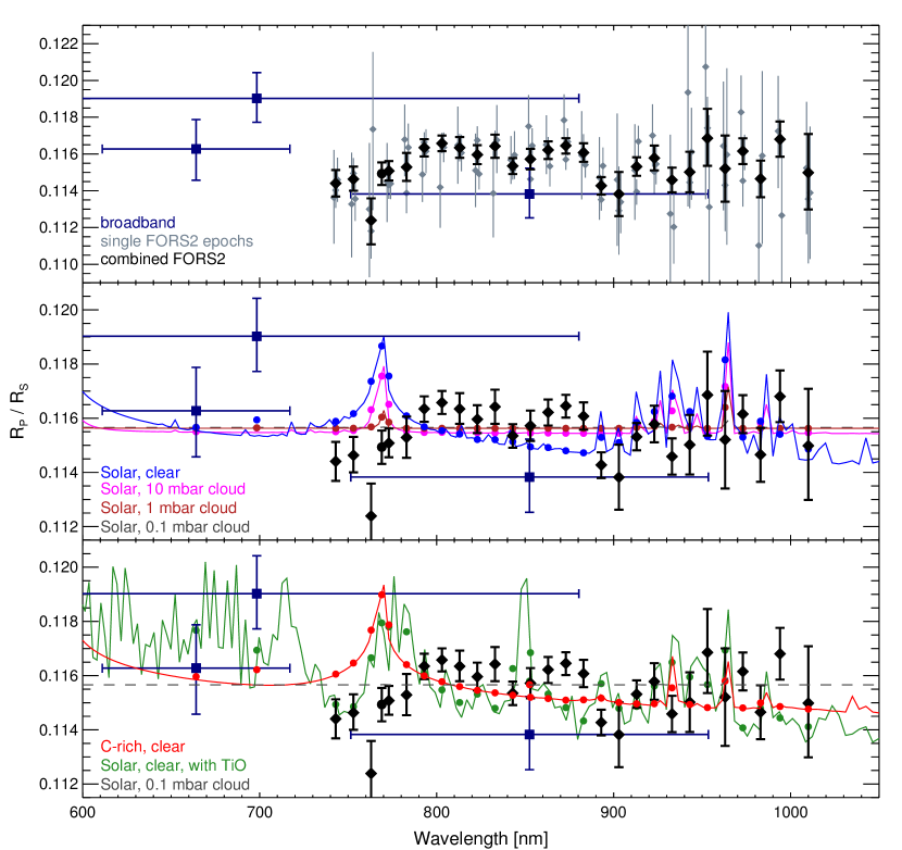
Figure 11: Transmission spectrum of WASP-49b as observed with FORS2, EulerCam and TRAPPIST compared to atmospheric models. Top: the FORS2 results of each separate data set are shown in gray and the results from the combined analysis are shown as black diamonds. The filled circle represents the data point centered on the K feature, and the results from broadband light curves are shown as dark blue squares. Center and bottom: the above transmission spectrum including the combined FORS2 and broadband data, together with predictions from atmosphere models. The model atmospheres are a clear solar-composition atmosphere (center panel, blue), a solar-composition atmosphere with a cloud deck at 10 mbar pressure (central panel, magenta), a solar-composition atmosphere with a cloud deck at 1 mbar pressure (central panel, dark red), a clear C-rich atmosphere (bottom panel, red), and a clear solar-composition atmosphere with TiO (bottom panel, green). A flat spectrum obtained from a solar-composition atmosphere with a cloud deck at 0.1 mbar pressure is shown as a gray dashed line in the middle and bottom panels. The filled circles show the models binned to the observed spectral resolution.

5 Conclusions

We have obtained a transmission spectrum of WASP-49b based on VLT/FORS2 observations of three planetary transits. The FORS2 data are affected by considerable systematic noise due to LADC inhomogeneities, but this noise is limited for observations where the LADC prism separation was set to a minimum and kept constant throughout the observation. We found consistent results from all three dates only when we applied a common noise model for light curve sets showing similar correlated noise together with low-order polynomial baselines to model each light curve’s large-scale trends individually. We therefore warn against the “blind” use of white light curve residuals alone to model spectrophotometric light curves that are affected with substantial correlated noise.

Using these data, we also updated the system parameters by taking contamination from a newly discovered nearby star into account. Our data agree with the previously published values while favoring a slightly larger planetary radius ($1.198_{-0.045}^{+0.047}$ ${R}_{J}$ instead of $1.115\pm 0.047$ ${R}_{J}$) and hence a lower planetary bulk density ($0.229\pm 0.016$ $\rho_{J}$ instead of $0.273^{+0.030}_{-0.026}$ $\rho_{J}$). The transmission spectra we obtain from the three epochs agree well with each other, demonstrating the instrumental stability and usefulness of FORS2 for high-precision spectrophotometry even in the presence of LADC-induced correlated noise.

We found that the transmision spectrum of WASP-49b is best fit by models with muted spectral features, such as expected in the presence of opaque high-altitude clouds or hazes. A carbon-rich atmosphere provides a comparable fit only when data at $\lambda<788$ nm are removed from the analysis. Solar-composition atmospheres, both with and without TiO are a poor match to the data. We conclude that WASP-49b most likely has clouds or hazes at pressure levels of 1 mbar or less.