Compton scattering $S$-matrix and cross section in strong magnetic field

Abstract

Compton scattering of polarized radiation in a strong magnetic field is considered. The recipe for calculation of the scattering matrix elements, the differential and total cross sections based on quantum electrodynamic (QED) second order perturbation theory is presented for the case of arbitrary initial and final Landau level, electron momentum along the field and photon momentum. Photon polarization and electron spin state are taken into account. The correct dependence of natural Landau level width on the electron spin state is taken into account in general case of arbitrary initial photon momentum for the first time. A number of steps in calculations were simplified analytically making the presented recipe easy-to-use. The redistribution functions over the photon energy, momentum and polarization states are presented and discussed. The paper generalizes already known results and offers a basis for accurate calculation of radiation transfer in strong $B$-field, for example, in strongly magnetized neutron stars.

I Introduction

Compton scattering is one of the most important processes of the interaction between radiation and matter in a number of astrophysical objects. Strong external magnetic field significantly affects the properties of the scattering (Harding and Lai, 2006): the interaction cross section becomes strongly dependent on energy, direction of photon momentum and polarization. It also depends on the magnetic field strength. A number of resonances corresponding to electron transition between the Landau levels appear. The resonant cross section value may exceed the Thomson scattering cross section $\sigma_{\rm T}$ by more than a factor of $10^{6}$. All these factors have to be taken into account in the studies of radiation transfer and interaction between radiation and matter in strongly magnetized medium. Finally, Compton scattering plays a key role in formation of spectra from magnetized neutron star atmospheres (Nagase et al., 1991; Ho and Lai, 2003; Watts et al., 2010; Suleimanov et al., 2009; Poutanen et al., 2013; van Putten et al., 2013) and dynamics of accretion onto magnetized neutron stars (Gnedin and Sunyaev, 1973; Mitrofanov and Pavlov, 1982; Mushtukov et al., 2015a; Tsygankov et al., 2006; Staubert et al., 2007).

The simplest expressions for Compton scattering cross-section in strong $B$-field was derived in non-relativistic limit by Canuto Canuto et al. (1971) and by Blandford & Scharlemann Blandford and Scharlemann (1976). The non-relativistic treatment is limited to dipole radiation and therefore only scattering at the cyclotron fundamental is allowed. The non-relativistic approach works well when $k\gamma\ll m_{\rm e}c^{2}$, where $k$ is a photon energy, $m_{\rm e}$ and $\gamma$ are the electron rest mass and the Lorentz factor respectively. At higher energies the relativistic effects become important for calculations of the scattering cross section (Klein and Nishina, 1929; Tamm, 1930) and kinematics (Rybicki and Lightman, 1979). The non-relativistic treatment is also limited to the magnetic field strength of $B\lesssim 10^{12}\,{\rm G}$ because the electron recoil becomes significant for higher $B$ (Daugherty and Ventura, 1978).

The relativistic quantum electrodynamics (QED) treatment allows us to describe scattering at higher harmonics and also consider the scattering which leads to electron transition to higher levels (so-called Raman scattering). It is the only way to describe scattering at high energies and strong magnetic field $B\gtrsim 10^{12}\,{\rm G}$, which is typical for young neutron stars.

The motion of electrons normal to the magnetic field is quantized in discrete Landau levels, whereas the longitudinal momentum can change continuously. The particular case of Compton scattering with both initial and final electrons on the ground Landau level of zero initial velosity was discussed by Herold Herold (1979). The scattering cross section from the ground to the arbitrary exited state was calculated by Daugherty & Harding Daugherty and Harding (1986) and by Meszaros Mészáros (1992). However, these QED calculations assume infinitely long-lived intermediate state and, therefore, are more relevant to photon energies far from the resonances. In order to calculate the resonant cross section one has to introduce a finite lifetime or decay width to the virtual electrons for cyclotronic transitions to lower Landau levels (Pavlov et al., 1991). For the specific case of ground-state to ground-state transition in the electron rest frame, when incident photons are parallel to the $B$-field, Gonthier et al. (Gonthier et al., 2014) showed that the commonly used spin-average width of Landau levels does not correctly account for the spin dependence of the temporal decay and results in a wrong value of the cross section at the resonance as well as at very low photon energies, where the level width becomes comparable to the energy of the initial photon.

Scattering from the ground Landau level is commonly used as a basic approach in case of a strong field: $\hbar eB/(m_{\rm e}c)>k_{\rm B}T$, where $k_{\rm B}$ is the Boltzmann constant and $T$ is the electron temperature, when the majority of electrons occupy the ground energy level (Pavlov et al., 1989; Nagase et al., 1991; Baring and Harding, 2007; Nobili et al., 2008; Watts et al., 2010; Chistyakov and Rumyantsev, 2006; Poutanen et al., 2013; Mushtukov et al., 2015a, b). For the case of initial electron on the ground Landau level and the initial photon with momentum parallel to the magnetic field direction, the cross section has only one resonance and takes the simplest form. A simple approximation for the scattering cross section in this case was found by Gonthier et al. Gonthier et al. (2000). Their approximation represents the exact cross section quite well below the resonance and above it even for extremely strong fields ($B<10^{15}\,{\rm G}$).

Moving electrons scatter the photons differently because of relativistic effects. As a result, the electron distribution over momentum affects the exact cross section and broadens the resonance features. This effect could be important for formation of spectral features in X-ray pulsars Nishimura (2008, 2011) and for the estimations of radiation pressure (Gnedin and Sunyaev, 1973; Mitrofanov and Pavlov, 1982; Mushtukov et al., 2015a), because the resonant scattering increases the effective interaction cross section dramatically. It is also important to use correct Landau level width and calculate correctly the exact resonant cross section here. The influence of electron distribution varies much with the photon momentum direction because electrons take part mostly in a motion along the $B$-field lines and the corresponding Doppler broadening varies a lot Harding and Daugherty (1991); Mushtukov et al. (2012). The scattering cross section for the case of thermal electrons was calculated and compared with cyclotron absorption by Harding & Daugherty Harding and Daugherty (1991). However, only polarization-averaged cross section for the case of initial electron at rest in the ground state was explored and an incorrect width of Landau levels based on Johnson-Lippmann wave-functions (Johnson and Lippmann, 1949) was taken into account (see (Herold et al., 1982) and (Gonthier et al., 2014) for detailed discussion).

Description of additional effects such as vacuum polarization, two-photon scattering (Berestetskii et al., 1971), pair creation Weise (2014) demands the use of high order perturbation theory. They are beyond the scope of the present work. However, it has to be pointed that the multiple photon scattering might be considered approximately as a chain of several elementary scatterings Bussard et al. (1986). Nevertheless, true scattering with an emission of two or more photons is a possibility which is given by QED treatment solely and the correct scattering cross section can be obtained only with relativistic treatment (Alexander and Meszaros, 1991; Semionova and Leahy, 2000).

According to QED, the scattering process is described completely by its scattering matrix ($S$-matrix) (Blandford and Scharlemann, 1976; Berestetskii et al., 1971), which contains the information about the probability amplitudes for the scattering. The transition probabilities and the effective cross sections of the various possible scattering are obtained from the $S$-matrix elements (which are complex numbers in general) as its squares, and therefore contain less information. The scattering cross sections are sufficient for a number of aims though, but the complete $S$-matrix is needed for general relativistic kinetic equation obtained recently by Mushtukov et al. (Mushtukov et al., 2012).

In this paper we give a detailed scheme of calculation of Compton scattering $S$-matrix elements, the differential and the total cross-section based on the QED second order perturbation theory. Some steps were done analytically simplifying the calculations significantly and making them easy-to-use. The scheme is valid for arbitrary initial and final Landau level, though we focused on the scattering from the ground Landau level only. For the first time calculations do not assume restrictions on the photon momentum and electron distribution over momentum. As a result, the scheme could be applied to direct calculations of scattering by moving electrons, which is important for modeling of interaction between radiation and matter in the vicinity of accreting highly magnetized neutron stars (Basko and Sunyaev, 1975; Becker and Wolff, 2007; Mushtukov et al., 2015a, c). The correct electron spin dependent Landau levels width (Herold et al., 1982; Latal, 1986; Pavlov et al., 1991) based on the Sokolov & Ternov electron eigenfunctions of the magnetic Dirac equation Sokolov and Ternov (1968, 1986) for the first time is taken into account in a general case of arbitrary initial photon momentum. The correct spin dependent width was already used in calculations of Compton scattering cross section for the particular case of photons initially propagating along the magnetic field and ground-to-ground state transition of the electron (Gonthier et al., 2014). In our calculations we generalize this result. The correct Landau levels width is shown to be particularly important if we are interested in polarization of scattered photons and accurate scattering cross section at the resonant energies (Gonthier et al., 2014). The obtained relations are valid in case of the magnetic field strength up to $\sim 10^{16}\,{\rm G}$ according to methods of particle description which are used in this paper (see Section II). We also discuss the redistribution function for the scattering (see Section VIII.2), which traditionally are used in radiation transfer equations and have a key role for studying the formation of spectral features near the cyclotron fundamental and its harmonics (Garasyov et al., 2011; Serber, 2000). We provide a scheme of calculation of the cross section for the case of scattering by an ensemble of electrons described by any distribution function over momentum. The results could be used for the solution of the kinetic equation for Compton scattering obtained by Pavlov et al. Pavlov et al. (1989) and generalized by Mushtukov et al. Mushtukov et al. (2012). Since the general relativistic kinetic equation can be expressed via $S$-matrix elements only, we discuss some properties of scattering matrix elements which are important for the kinetic theory (see Section VII). The paper describes the most general scheme for Compton scattering calculation in strong magnetic field based on the second order of QED perturbation theory and provides a ground for detailed investigation in a field of radiation transfer in case of strong external magnetic field.

We do not discuss here an influence of plasma effects on Compton scattering. The description of plasma effects was given in number of works (Bulik and Miller, 1997; Chistyakov et al., 2012).

For simplicity we use the relativistic quantum system of units where the Planck constant, speed of light and the electron mass are equal unity: $\hbar=c=m_{\rm e}=1$. In this case the length unit is Compton wavelength $\lambda\hskip-5.0pt\raise 3.0pt\hbox{--}_{\rm C}=\hbar/m_{\rm e}c$, the unit of energy is the electron rest mass energy $m_{\rm e}c^{2}$, the frequency unit is $m_{\rm e}c^{2}/\hbar$ and momentum is measured in $m_{\rm e}c$. The electron charge is $e=\sqrt{1/137.036}$. The classical electron radius $r_{\rm e}$ is equal to the fine-structure constant $\alpha_{\rm fs}$ in using system of units: $r_{\rm e}=e^{2}/(m_{\rm e}c^{2})=e^{2}/(\hbar c)=\alpha_{\rm fs}=1/137.036$.

II Particle description

Let us consider constant and uniform magnetic field. The field is directed along the $z$-axis and could be represented by 3-dimensional vector $\textbf{{B}}_{\rm e}=B_{\rm e}\,(0,0,1),$ where $B_{\rm e}>0$ is the field strength. Let us also use dimensionless magnetic field strength $b=B_{\rm e}/B_{\rm cr}$, which is a strength measured in units of the Schwinger critical value $B_{\rm cr}=m^{2}_{\rm e}c^{3}/e\hbar=4.412\times 10^{13}$G.

II.1 Electron in a strong magnetic field

According to quantum mechanics the kinetic energy of the transverse motion is quantized in Landau levels (Landau and Lifshit’s, 1991), since the particles gyrate in circular orbits. Each electron is described by a set of quantum numbers which includes the Landau level number $n=0,1,2,...$, $z$-projection of electron momentum $p_{z}$, $y$-projection of electron momentum $p_{y}$ and electron spin projection onto the $z$-axis measured in $\hbar/2$-units $s=\pm 1$. We also use quantum number $\varepsilon$ to describe the electron anti-particle - positron, $\varepsilon=1$ for electrons and $\varepsilon=-1$ for positrons. All Landau levels except the ground one ($n=0$) are degenerate with the spin-projection $s=\pm 1$. For the ground Landau level the spin degeneracy is one: $s=-1$.

The total electron energy in $B$-field with strength $b$ is defined by the Landau level number $n$ and $z$-projection of the electron momentum $p_{z}$:

$$E_{n}(Z)=\sqrt{1+p_{z}^{2}+2\,b\,n}.$$ (1)

According to relativistic quantum theory the electron states in external magnetic field are described by solutions of Dirac equation $\Psi_{n\,s}^{\varepsilon}(\underline{r},p_{y},p_{z})$ enumerated by given quantum numbers (see Appendix D). The solutions could be written in different ways. They could be found via the eigenfunctions of a spin operator in the reference frame where the spin direction is fixed (Kuznetsov and Mikheev, 2003). In this case it is impossible to construct the Lorentz invariant amplitude for the processes with definite electron spin state since the spin direction is fixed. At the same time the amplitudes which are summed over the electron spin states are Lorentz invariant. The solutions could be also found as the eigenfunctions of the operator $\hat{\mu}_{z}=m_{\rm e}\Sigma_{z}-{i}\gamma_{0}\gamma_{5}[\boldsymbol{\Sigma}\times\hat{p}]_{z}$, where $\hat{p}=-{i}{\bf\nabla}-e\underline{A}_{\rm e}$ is the generalized momentum operator and $\underline{A}_{\rm e}=B_{\rm e}(0,0,x,0)$ is 4-potential in Landau gauge (Sokolov and Ternov, 1986) (see Appendix C for all necessary definitions). In this case the amplitudes for spin dependent processes are manifestly Lorentz-invariant (Kuznetsov et al., 2013). Nevertheless, one could use both ways in case when we are interested only in the state averaged over the electron spin state. We discuss how to construct the electron wave function in Appendix D.

Further we will use following designations:

$$b_{n}=\sqrt{2\,b\,n},\,\,s_{n}=\sqrt{1+b_{n}^{2}}=\sqrt{1+2\,b\,n},\,\,E_{n}(p_{z})=\sqrt{s_{n}^{2}+p_{z}^{2}}.$$ (2)

Let us choose that the laboratory reference frame as a frame where the initial electron has zero-velocity. Lorentz transformation along the magnetic field direction provides the conversion from one inertial system to another.

II.2 Photon description

Each photon is described by its energy $k$, the momentum direction defined by the unit-vector $\boldsymbol{\omega}=(\sin\theta\,\cos\varphi,\sin\theta\,\sin\varphi,\cos\theta)$ and its polarisation state. The 3-dimensional photon momentum in Cartesian coordinates: $\textbf{{k}}=(k_{\rm x},k_{\rm y},k_{\rm z})=k\boldsymbol{\omega}$ and the corresponding photon 4-momentum: $\underline{k}=\{k,\textbf{{k}}\}$.

The photon propagation in strong magnetic field is affected by vacuum polarization effects. Since photons may temporarily convert into virtual electron-positron pairs, which are polarized by the $B$-field, the dielectric and permeability tensors of magnetised vacuum are nontrivial. As a result the photon phase and group velocity depends on the polarization (Mészáros, 1992; Kuznetsov and Mikheev, 2003), and it is natural to consider photons of two linear polarizations: $O$-mode (or $\|$-mode) photons which are linearly polarized in a plane containing $\boldsymbol{\omega}$ and B and $X$-mode (or $\perp$-mode) photons which are polarized perpendicularly.

The 4-vector potential for the photon can be defined as:

$$\underline{A}_{l}(\underline{r})=\underline{e}_{l}e^{-i\underline{k}\,\underline{r}},\quad\underline{e}_{l}=\{0,\textbf{{e}}_{l}\},\quad l=1,2.$$ (3)

The photon polarization is described in the co-ordinates which are specified by unit-vector $\boldsymbol{\omega}$ and two additional basis vectors: $\textbf{{e}}_{1}=(\sin\varphi,-\cos\varphi,0)$ and $\textbf{{e}}_{2}=(\cos\theta\cos\varphi,\cos\theta\sin\varphi,-\sin\theta)$. It is convenient to use so-called cyclic coordinates instead of Cartesian ones. The $z$-projection would be the same in this case, but

$$e_{1,\pm}=\sin\varphi\mp i\cos\varphi=\mp ie^{\pm i\varphi},\,\,e_{2,\pm}=\cos\theta(\cos\varphi\pm i\sin\varphi)=\cos\theta e^{\pm i\varphi}$$ (4)

are used instead of $x$- and $y$-projections. Thus, the coordinates of polarization basic vectors ($e_{\rm z},\,e_{+},\,e_{-}$) in cyclic coordinates are

$$\textbf{{e}}_{1}(\textbf{{k}})=(0,-ie^{i\varphi},ie^{-i\varphi}),\quad\textbf{{e}}_{2}(\textbf{{k}})=(-\sin\theta,\cos\theta e^{i\varphi},\cos\theta e^{-i\varphi}),\quad\textbf{{e}}_{3}(\textbf{{k}})=(\cos\theta,\sin\theta e^{i\varphi},\sin\theta e^{-i\varphi}).$$ (5)

The condition of orthonormality is $\textbf{{e}}_{l}(\textbf{{k}})\textbf{{e}}_{l_{1}}^{*}(\textbf{{k}})=\delta_{l\,l_{1}}$.

The photons are described here in the same manner as in case when the magnetic field is absent, i.e. we assume that the dispersion relation for the photons in magnetized vacuum does not differ from the dispersion relation for field absent case. This approximation constrains the strength of the field. For estimations one needs to know vacuum dielectric tensor and the inverse permeability tensor for the case of magnetized vacuum (Adler, 1971; Potekhin et al., 2004) but it is known that the indices of refraction differ from unity by more than $10\%$ only for the fields hundred times stronger than the critical magnetic field, $b>300$ (Shaviv et al., 1999). Thus, it restricts application of the developed formalism to $B\lesssim 10^{16}$G.

III Conservation laws and their consequences

There are only three conservation laws for Compton scattering in strong $B$-field. It is the energy conservation law and the laws of longitudinal and transversal momentum conservation:

$$E_{i}+k_{i}=E_{f}+k_{f},\,\,\,\,p_{z,i}+k_{i}\cos\theta_{i}=p_{z,f}+k_{f}\cos\theta_{f},\,\,\,\,p_{y,i}+k_{i}\sin\theta_{i}\sin\varphi_{i}=p_{y,f}+k_{f}\sin\theta_{f}\sin\varphi_{f},$$ (6)

where quantities which are corresponding to the initial particle states are denoted with the index ”${i}$” while the quantities which are describing the final particle states are indexed with ”${f}$”.

In order to define the scattering event one has to define all quantum numbers which correspond to the particles in the initial and final states. The quantum numbers should comply with conservation laws (6). One possible way is to define all initial particle parameters and some final parameters. The initial condition of a system could be defined by $p_{z,i},\,n_{i},\,k_{i}$, two angles $\theta_{i},\,\varphi_{i}$, and also by photon and electron polarization states. All other quantum number can be found from conservation laws (6). If one specifies the final Landau level $n_{f}$, then the final photon energy $k_{f}$ and the zenith angle $\theta_{f}$ comply with the following relation:

$$k^{2}_{f}\sin^{2}\theta_{f}-2k_{f}(E_{\rm T}-Z_{\rm T}\cos\theta_{f})+\left[E^{2}_{\rm T}-Z^{2}_{\rm T}-(1+2bn_{f})\right]=0,$$

where $E_{\rm T}\equiv E_{i}+k_{i}=E_{f}+k_{f}$ is the total energy and $Z_{\rm T}=Z_{i}+k_{i}\cos\theta_{i}=Z_{f}+k_{f}\cos\theta_{f}$ is the total longitudinal momentum of electron-photon system. In this case, the energy of the final photon is

$$k_{f}=\frac{k_{i}\left[k_{i}\sin^{2}\theta_{i}+2(E_{i}-p_{z,i}\cos\theta_{i})\right]+2b(n_{i}-n_{f})}{E_{\rm T}-Z_{\rm T}\cos\theta_{f}+(E_{\rm T}\cos\theta_{f}-Z_{\rm T})^{2}+s^{2}_{f}\sin\theta_{f}}.$$ (7)

Because the photon energy should be positive, there exist a limit on the final Landau level number:

$$n_{f}\leq n_{f}^{0}=n_{i}+\lfloor k_{\rm R}/2b\rfloor,$$ (8)

where $\lfloor x\rfloor$ is a floor function of $x$ and $k_{\rm R}=k_{i}\left(k_{i}\sin^{2}\theta_{i}+2(E_{i}-p_{z,i}\cos\theta_{i})\right)$. Thus, the given initial photon ($k_{i},\,\theta_{i}$) and electron ($p_{z,i},\,n_{i}$) parameters with the final Landau level number $n_{f}$ define uniquely the final photon energy in any direction.

IV Matrix elements for Compton scattering

According to QED, Compton scattering is a second-order process and is described by two Feynman diagrams (Fig.1). Both of them contain photon and electron before and after the interaction. The diagrams also contain so-called virtual electron/positron for which energy and momentum are not strictly conserved.

Figure 1: Two second order Feynman diagrams for Compton scattering. Wavy and streight lines depict photons and electrons/positrons correspondingly. The streight line between two vertices corresponds to a virtual particle.

Following the Feynman rules one gets elements of $S$-matrix for the process, which is the first step towards obtaining cross section (Berestetskii et al., 1971). The initial electron is described by a particular solution of the Dirac equation for the electron in external magnetic filed $\Psi_{i}^{+}(\underline{r}_{1})=\Psi_{n_{i}s_{i}}^{+}(\underline{r}_{1},p_{y,i},p_{z,i})$ (see Section D.5). The final electron is also described by one of the solutions $\Psi_{f}^{+}(\underline{r}_{2})=\Psi_{n_{f}s_{f}}^{+}(\underline{r}_{2},p_{y,f},p_{z,f})$. The photons are described by 4-vectors of potential: $A_{i}(\underline{r}),\,\,A_{f}(\underline{r})$ (see equation (3)). The interaction in a point $\underline{r}$ gives us $e\underline{\gamma}\underline{A}(\underline{r})\Psi^{+}(\underline{r})$ according to the Feynman rules. The initial states give $e\underline{\gamma}\underline{A}_{i}(\underline{r})$ and $\Psi^{+}_{i}(\underline{r})$, while the final ones give $e\underline{\gamma}\underline{A}_{f}^{\dagger}(\underline{r})$ and $\Psi_{f}^{+\dagger}(\underline{r})\gamma^{0}=\overline{\Psi}_{f}^{+}(\underline{r})$.

An internal electron line corresponds to the virtual electron state. The line begins in point $\underline{r}_{1}$, and ends in point $\underline{r}_{2}$. The virtual particle is described by the relativistic propagator $G(\underline{r},\underline{r}_{1})$, which is a Green’s function of the Dirac equation:

$$\left[(i\underline{\bigtriangledown}+e\underline{A}_{\rm e})\underline{\gamma}-1\right]G(\underline{r},\underline{r}_{1})=\delta(\underline{r}-\underline{r}_{1}).$$ (9)

It takes the following form for the case of electron in strong $B$-field:

$$G(\underline{r}_{2},\underline{r}_{1})=-{i}\sum_{n,\varepsilon,s}\int{\rm d}p_{y}\,{\rm d}p_{z}\Psi_{ns}^{\varepsilon}(\textbf{{r}}_{2},t_{2},p_{y},p_{z})\overline{\Psi}_{ns}^{\,\varepsilon}(\textbf{{r}}_{1},t_{1},p_{y},p_{z})\,\varepsilon\,\Theta(\varepsilon\,(t_{2}-t_{1})),$$ (10)

where $\Theta(x)$ is the Heaviside step function. The same expression could be written in details as

$$\displaystyle G(\underline{r}_{2},\underline{r}_{1})=-\frac{i}{(2\pi)^{2}}\int\limits_{-\infty}^{\infty}{\rm d}p_{z}e^{i\varepsilon p_{z}(z_{2}-z_{1})}\int\limits_{-\infty}^{\infty}{\rm d}p_{y}e^{i\varepsilon p_{y}(y_{2}-y_{1})}\sum_{n=0}^{\infty}\sum_{s=\pm 1}\sum_{\varepsilon=\pm 1}\frac{1}{E_{n}(p_{z})}$$ (11)

$$\displaystyle\times e^{i\varepsilon E_{n}(p_{z})(t_{1}-t_{2})}v_{ns}^{\varepsilon}(\varepsilon p_{z},x+\varepsilon p_{y}/b)v_{ns}^{\varepsilon\dagger}(\varepsilon p_{z},x+\varepsilon p_{y}/b)\gamma^{0}\varepsilon\Theta(\varepsilon(t_{2}-t_{1})),$$

where the terms without any indexes correspond to the virtual electron/positron and one has to sum over the quantum numbers $n$ (Landau level) and $s$ (spin state).

Finally, the matrix element for Compton scattering which corresponds to the first two Feynman diagrams takes the following form:

$$S_{{f}{i}}=-4\pi ir_{\rm e}\int{\rm d}^{4}r_{1}\,{\rm d}^{4}r_{2}\overline{\Psi}_{f}^{+}(\underline{r}_{2})\left\{\left[\underline{\gamma}\underline{A}_{f}^{\dagger}(\underline{r}_{2})\right]\,G(\underline{r}_{2},\underline{r}_{1})\left[\,\underline{\gamma}\underline{A}_{i}(\underline{r}_{1})\right]+\left[\,\underline{\gamma}\underline{A}_{i}(\underline{r}_{2})\right]\,G(\underline{r}_{2},\underline{r}_{1})\left[\underline{\gamma}\underline{A}_{f}^{\dagger}(\underline{r}_{1})\right]\right\}\Psi_{i}^{+}(\underline{r}_{1}).$$ (12)

The first term in curly brackets corresponds to the a-diagram, while the second one corresponds to the b-diagram (Fig.1).

V Simplification and some algebra

The general expression for the $S$-matrix element (12) has to be specified. New expression for the elements will contain integrals over time and space variables and sums over the discrete virtual electron/positron quantum numbers. It will be shown that the integrals could be calculated analytically as well as some sums. As a result we will get relatively simple expression for the elements of $S$-matrix, which would be suitable for the further analysis.

V.1 First steps and integration over momentum and time variables

Using the expression for the electron propagator (11) and the general expression for the $S$-matrix elements (12) we rewrite $S$-matrix elements in the following form:

$$\displaystyle S_{{f}{i}}\!=\!-4\pi r_{\rm e}\int{\rm d}^{4}r_{1}\,{\rm d}^{4}r_{2}\sum_{n,\varepsilon\,s}\int{\rm d}p_{y}{\rm d}p_{z}\Psi_{n_{f}\,s_{f}}^{+\dagger}(\underline{r}_{2},p_{y,f},p_{z,f})\{[\gamma^{0}\underline{\gamma}\underline{A}_{f}^{\dagger}(\underline{r}_{2})]\,\Psi_{n\,s}^{\varepsilon}(\underline{r}_{2},p_{y},p_{z})\Psi_{n\,s}^{\varepsilon\dagger}(\underline{r}_{1},p_{y},p_{z})[\gamma^{0}\underline{\gamma}\underline{A}_{i}(\underline{r}_{1})]$$ (13)

$$\displaystyle+[\gamma^{0}\underline{\gamma}\underline{A}_{i}(\underline{r}_{2})]\,\Psi_{n\,s}^{\varepsilon}(\underline{r}_{2},p_{y},p_{z})\Psi_{n\,s}^{\varepsilon\dagger}(\underline{r}_{1},p_{y},p_{z})[\gamma^{0}\underline{\gamma}\underline{A}_{f}^{\dagger}(\underline{r}_{1})]\}\Psi^{+}_{n_{i}\,s_{i}}(\underline{r}_{1},p_{y,i},p_{z,i})\varepsilon\Theta(\varepsilon(t_{2}-t_{1})).$$

We have also changed Dirac conjugated functions with the Hermit conjugated and $\gamma^{0}$ matrix has appeared as a result (see Appendix C). Using the expressions which are describing the electron (see Section D) and photon states we get:

$$\displaystyle S_{{f}{i}}=-4\pi r_{\rm e}\sum_{n,\varepsilon,s}\int{\rm d}p_{y}{\rm d}p_{z}\int{\rm d}^{4}r_{1}\,{\rm d}^{4}r_{2}\frac{\varepsilon\Theta(\varepsilon(t_{2}-t_{1}))}{(2\pi)^{2}R_{n}}\frac{1}{2\pi\sqrt{R_{f}}}v_{n_{f}\,s_{f}}^{+\dagger}(p_{z,f},x_{2}+p_{y,f}/b)e^{i(E_{f}t_{2}-p_{y,f}y_{2}-p_{z,f}z_{2})}$$

$$\displaystyle\times\left\{[\gamma^{0}\underline{\gamma}\underline{e}_{l_{f}}]e^{ik_{f}(t_{2}-\boldsymbol{\omega}_{f}\textbf{{r}}_{2})}v_{n\,s}^{\varepsilon}(\varepsilon p_{z},x_{2}+\varepsilon p_{y}/b)v_{n\,s}^{\varepsilon\dagger}(\varepsilon p_{z},x_{1}+\varepsilon p_{y}/b)[\gamma^{0}\underline{\gamma}\underline{e}_{l_{i}}]e^{-ik_{i}(t_{1}-\boldsymbol{\omega}_{i}\textbf{{r}}_{1})}\right.$$

$$\displaystyle\left.+[\gamma^{0}\underline{\gamma}\underline{e}_{l_{i}}]e^{-ik_{i}(t_{2}-\boldsymbol{\omega}_{i}\textbf{{r}}_{2})}v_{n\,s}^{\varepsilon}(\varepsilon Z,x_{2}+\varepsilon p_{y}/b)v_{n\,s}^{\varepsilon\dagger}(\varepsilon p_{z},x_{1}+\varepsilon p_{y}/b)[\gamma^{0}\underline{\gamma}\underline{e}_{l_{f}}]e^{ik_{f}(t_{1}-\boldsymbol{\omega}_{f}\textbf{{r}}_{1})}\right\}$$ (14)

$$\displaystyle\times\frac{1}{2\pi\sqrt{E_{i}}}\,v_{n_{i}\,s_{i}}^{+}(p_{z,i},x_{1}+p_{y,i}/b)e^{-i(E_{i}t_{1}-p_{y,i}y_{1}-p_{z,i}z_{1})}e^{\varepsilon i[-E_{n}(t_{2}-t_{1})+p_{y}(y_{2}-y_{1})+p_{z}(z_{2}-z_{1})]}.$$

Taking the integrals over $y_{1},y_{2},z_{1},z_{2}$ we get two products of $(2\pi)^{4}$ with four $\delta$-functions which are correspond to the momentum conservation in the Feynman diagram vertices. For the first term (a-diagram) we set $\delta(\varepsilon p_{y}-p_{y,f}-k_{{f}{\rm y}})\,\delta(p_{y,i}+k_{{i}{\rm y}}-\varepsilon p_{y})\,\delta(\varepsilon p_{z}-p_{z,f}-k_{{f}{\rm z}})\,\delta(p_{z,i}+k_{{i}{\rm z}}-\varepsilon p_{z})$, while for the second one (b-diagram) we have $\delta(\varepsilon p_{y}-p_{y,f}+k_{{i}{\rm y}})\,\delta(p_{y,i}-k_{{f}{\rm y}}-\varepsilon p_{y})\,\delta(\varepsilon p_{z}-p_{z,f}+k_{{i}{\rm z}})\,\delta(p_{z,i}-k_{{f}{\rm z}}-\varepsilon p_{z})$. $(2\pi)^{4}$ has vanished. The integrals over $p_{y}$ and $p_{z}$ could be taken easily because of $\delta$-functions under the integrals. Finally, we are left with the product of two $\delta$-function $\delta(p_{y,i}+p_{y,f}-k_{{i}{\rm y}}-k_{{f}{\rm y}})\delta(p_{z,i}+p_{z,f}-k_{{i}{\rm z}}-k_{{f}{\rm z}})$, which describe the conservation laws for the momentum. The values of $\varepsilon p_{z}$ and $\varepsilon p_{y}$ for the virtual electron are different for two Feynman diagrams. Let us denote them with indexes ”a” and ”b” respectively:

$$\displaystyle Z_{\rm a}=p_{z,i}+k_{{i}{\rm z}}=p_{z,f}+k_{{f}{\rm z}},\,\,\,\,\,Y_{\rm a}=p_{y,i}+k_{{i}{\rm y}}=p_{y,f}+k_{{f}{\rm y}},$$ (15)

$$\displaystyle Z_{\rm b}=p_{z,i}-k_{{f}{\rm z}}=p_{z,f}-k_{{i}{\rm z}},\,\,\,\,\,Y_{\rm b}=p_{y,i}-k_{{f}{\rm y}}=p_{y,f}-k_{{i}{\rm y}}.$$

The virtual electron energy would be also different for two diagrams: $E_{n{\rm a}}=\sqrt{s_{n}^{2}+Z_{\rm a}^{2}}$ and $E_{n{\rm b}}=\sqrt{s_{n}^{2}+Z_{\rm b}^{2}}$.

Thus, the expression for the matrix element (V.1) takes the form:

$$\displaystyle S_{{f}{i}}=-4\pi r_{\rm e}\delta(p_{y,f}+k_{{f}{\rm y}}-p_{y,i}-k_{{i}{\rm y}})\delta(p_{z,f}+k_{{f}{\rm z}}-p_{z,i}-k_{{i}{\rm z}})\sum_{n,\varepsilon,s}\int{\rm d}x_{1}{\rm d}x_{2}{\rm d}t_{1}{\rm d}t_{2}\frac{\varepsilon\Theta(\varepsilon(t_{2}-t_{1})}{\sqrt{E_{i}E_{f}}}$$

$$\displaystyle\times v_{n_{f}\,s_{f}}^{+\dagger}(p_{z,f},x_{2{f}})\left\{e^{i[(E_{f}+k_{f}-\varepsilon E_{n{\rm a}})t_{2}+(\varepsilon E_{n{\rm a}}-k_{i}-E_{i})t_{1}]}M_{l_{f}}v_{ns}^{\varepsilon}(Z_{\rm a},x_{2{\rm a}})v_{ns}^{\varepsilon\dagger}(Z_{\rm a},x_{1{\rm a}})M_{l_{i}}e^{i(k_{{i}{\rm x}}x_{1}-k_{{f}{\rm x}}x_{2})}\right.$$

$$\displaystyle\left.+e^{i(k_{{i}{\rm x}}x_{2}-k_{{f}{\rm x}}x_{1})}e^{i[(E_{f}-k_{i}-\varepsilon E_{n{\rm b}})t_{2}+(\varepsilon E_{n{\rm b}}+k_{f}-E_{i})]}M_{l_{i}}v_{ns}^{\varepsilon}(Z_{\rm b},x_{2{\rm b}})v_{ns}^{\varepsilon\dagger}(Z_{\rm b},x_{1{\rm b}})M_{l_{f}}\right\}v_{n_{i}s_{i}}^{+}(p_{z,i},x_{1{i}}).$$ (16)

Here

$$M_{l}=-\gamma^{0}\underline{\gamma}\underline{e}_{l}=\boldsymbol{\alpha}\textbf{{e}}_{l}=\left(\begin{array}[]{cccc}0&0&e_{lz}&e_{l-}\\ 0&0&e_{l+}&-e_{lz}\\ e_{lz}&e_{l-}&0&0\\ e_{l+}&-e_{lz}&0&0\\ \end{array}\right),$$ (17)

where $l=1,2$ corresponds to photon polarization state and $\boldsymbol{\alpha}$ is given by equation (67). In particular cases of $X$- and $O$-mode photons the matrices take the form:

$$M_{1}=\left(\begin{array}[]{cccc}0&0&0&ie^{-i\varphi}\\ 0&0&-ie^{i\varphi}&0\\ 0&ie^{-i\varphi}&0&0\\ -ie^{i\varphi}&0&0&0\\ \end{array}\right),\quad M_{2}=\left(\begin{array}[]{cccc}0&0&-\sin\theta&\cos\theta e^{-i\varphi}\\ 0&0&\cos\theta e^{i\varphi}&\sin\theta\\ -\sin\theta&\cos\theta e^{-i\varphi}&0&0\\ \cos\theta e^{i\varphi}&\sin\theta&0&0\\ \end{array}\right).$$

In equations (V.1,V.1) we also used notations for the spinor argument:

$$\displaystyle x_{2\,{f}}=x_{2}+Y_{f}/b,\quad x_{2\,{\rm a}}=x_{2}+(p_{y,f}+k_{{f}{\rm y}})/b,\quad x_{2\,{\rm b}}=x_{2}+(p_{y,f}-k_{{i}{\rm y}})/b,$$ (18)

$$\displaystyle x_{1\,{i}}=x_{1}+p_{y,i}/b,\quad x_{1\,{\rm a}}=x_{1}+(p_{y,i}+k_{{i}{\rm y}})/b,\quad x_{1\,{\rm b}}=x_{1}+(p_{y,i}-k_{{f}{\rm y}})/b.$$ (19)

The next step is taking the integrals over time variables $t_{1}$ and $t_{2}$. Using the relation $\int_{0}^{\infty}e^{ixy}{\rm d}y=\pi\delta(x)+{i}/{x}$ one gets the following expression for the case of a-diagram:

$$\displaystyle\int\limits_{-\infty}^{\infty}{\rm d}t_{1}\int\limits_{-\infty}^{\infty}{\rm d}t_{2}e^{i[(E_{f}+k_{f}-\varepsilon E_{n{\rm a}})t_{2}+(\varepsilon E_{n{\rm a}}-k_{i}-E_{i})t_{1}]}\varepsilon\Theta(\varepsilon(t_{2}-t_{1}))$$

$$\displaystyle=2\pi\delta(E_{f}+k_{f}-E_{i}-k_{i})\left[\frac{i}{E_{i}+k_{i}-\varepsilon E_{n{\rm a}}}+\varepsilon\delta(E_{i}+k_{i}-\varepsilon E_{n{\rm a}})\right]=2\pi i\frac{\delta(E_{f}+k_{f}-E_{i}-k_{i})}{E_{i}+k_{i}-\varepsilon E_{n{\rm a}}},$$

and for b-diagram:

$$\displaystyle\int\limits_{-\infty}^{\infty}{\rm d}t_{1}\int\limits_{-\infty}^{\infty}{\rm d}t_{2}e^{i[(E_{f}-k_{i}-\varepsilon E_{n{\rm b}})t_{2}+(\varepsilon E_{n{\rm b}}+k_{f}-E_{i})t_{1}]}\varepsilon\Theta(\varepsilon(t_{2}-t_{1}))$$

$$\displaystyle=2\pi\delta(E_{f}+k_{f}-E_{i}-k_{i})\left[\frac{i}{E_{i}-k_{f}-\varepsilon E_{n{\rm b}}}+\varepsilon\delta(E_{i}-k_{f}-\varepsilon E_{n{\rm b}})\right]=2\pi i\frac{\delta(E_{f}+k_{f}-E_{i}-k_{i})}{E_{i}-k_{f}-\varepsilon E_{n{\rm b}}}.$$

The $\delta$-functions outside the square brackets correspond to the energy conservation law. The $\delta$-function arguments inside the brackets (as well as denominators) describe the relation between the virtual particle energy and real particle energies in the Feynman diagrams vertexes. These arguments are not equal to zero in general, but may have values close to zero. It leads to the appearance of the resonances and matrix elements as well as cross sections become infinite. The infinities are removed by the regularization procedure, when one takes into account the natural width of Landau levels Pavlov et al. (1991); Nagirner and Kiketz (1993) (see Section VI and Appendix B). In this case the denominators are small but nevertheless differ from zero and the cross section values are not infinite.

After the integration over time variable the $S$-matrix elements (V.1) take the final form:

$$\displaystyle S_{{f}{i}}=-8\pi^{2}ir_{\rm e}\delta(p_{y,f}+k_{{f}y}-p_{y,i}-k_{{i}y})\delta(p_{z,f}+k_{{f}z}-p_{z,i}-k_{{i}z})\delta(E_{f}+k_{f}-E_{i}-k_{i})$$ (20)

$$\displaystyle\times\sum_{n,\varepsilon,s}\int\frac{{\rm d}x_{1}{\rm d}x_{2}}{\sqrt{E_{i}E_{f}}}v_{n_{f}\,s_{f}}^{+\dagger}(p_{z,f},x_{2{f}})\left\{M_{l_{f}}v_{ns}^{\varepsilon}(Z_{\rm a},x_{2{\rm a}})v_{ns}^{\varepsilon\dagger}(Z_{\rm a},x_{1{\rm a}})M_{l_{i}}\frac{e^{i(k_{{i}x}x_{1}-k_{{f}x}x_{2})}}{E_{i}+k_{i}-\varepsilon E_{n{\rm a}}}\frac{1}{E_{n{\rm a}}}\right.$$

$$\displaystyle\left.+\frac{1}{E_{n{\rm b}}}\frac{e^{i(k_{{i}x}x_{2}-k_{{f}x}x_{1})}}{E_{i}-k_{f}-\varepsilon E_{n{\rm b}}}M_{l_{i}}v_{ns}^{\varepsilon}(Z_{\rm b},x_{2{\rm b}})v_{ns}^{\varepsilon\dagger}(Z_{\rm b},x_{1{\rm b}})M_{l_{f}}\right\}v_{n_{i}s_{i}}^{+}(p_{z,i},x_{1{i}}),$$

where the spinors $v^{\varepsilon}_{ns}$ are given by equations (110-113) (see Appendix D) and matrices $M_{l}$ are defined by equation (17). The braces in equation (20) contain $4\times 4$ matrices, while the whole construction under the integral is reduced to the complex function. The integration over $x_{1}$ and $x_{2}$ can be done analytically (see Section V.2) as well as summation over the energy sign $\varepsilon$ and spin state $s$ (see Section V.3). The summation over the electron spin states has to be done numerically.

V.2 An integration over space variable in $S$-matrix elements

Let us take the expressions for spinors $v^{\varepsilon}_{ns}$ (110-113) (see Appendix D) and use them in final expression for the $S$-matrix elements (20). Then the product of matrices $M_{l}$ and spinors $v^{\varepsilon}_{ns}$ under the integral in equation (20) is simplified and we are coming to the integrals which contain the products of $\chi$-function which are defined by equation (103). All the integrals have the same form and could be represented via the Hermite polynomials:

$$\displaystyle I_{l_{1}\,l_{2}}=\int\limits_{-\infty}^{\infty}{\rm d}x\chi^{*}_{l_{1}}(x+\alpha_{1})\chi^{\phantom{*}}_{l_{2}}(x+\alpha_{2})e^{i\alpha x}$$

$$\displaystyle=\frac{\sqrt{b}}{\sqrt{\pi}}\frac{i^{l_{2}-l_{1}}}{\sqrt{2^{l_{1}}l_{1}!2^{l_{2}}l_{2}!}}\int\limits_{-\infty}^{\infty}{\rm d}xe^{-b(x^{2}+2\alpha_{1}x+\alpha_{1}^{2}+x^{2}+2\alpha_{2}x+\alpha_{2}^{2})/2+i\alpha x}H_{l_{1}}(\sqrt{b}(x+\alpha_{1}))H_{l_{2}}(\sqrt{b}(x+\alpha_{2})).$$ (21)

With new variables $u=\sqrt{b}[x+(\alpha_{1}+\alpha_{2}-i\alpha/b)/2]$ the last expression could be rewritten as

$$I_{l_{1}\,l_{2}}=\frac{e^{\pi i(l_{2}-l_{1})/2}}{\sqrt{\pi 2^{l_{1}+l_{2}}l_{1}!l_{2}!}}\exp\left(-\frac{|\beta|^{2}}{4}-i\alpha\frac{\alpha_{1}+\alpha_{2}}{2}\right)\int\limits_{-\infty}^{\infty}{\rm d}u\,e^{-u^{2}}H_{l_{1}}\left(u+\frac{\beta^{*}}{2}\right)H_{l_{2}}\left(u-\frac{\beta}{2}\right),$$ (22)

where $\beta=\sqrt{b}(\alpha_{1}-\alpha_{2}-i\alpha/b)$. The integrals of the Hermitian polynomials product could be taken analytically and have well known expression through the Laguerre polynomials (Gradshteyn and Ryzhik, 1980):

$$\int\limits_{-\infty}^{\infty}{\rm d}u\,e^{-u^{2}}H_{n}(u+x)H_{m}(u+y)=2^{n}\sqrt{\pi}m!x^{n-m}L_{m}^{n-m}(-2xy),\,\,\,\,n\geq m.$$

In our case $n=\max(l_{1},l_{2})=\overline{l}$, $m=\min(l_{1},l_{2})=\underline{l}$, $n-m=\overline{l}-\underline{l}=|l_{1}-l_{2}|$, $xy=-|\beta|^{2}/4$, $x^{n-m}=(|\beta|/2)^{|l_{1}-l_{2}|}e^{i(l_{2}-l_{1})\arg\beta}e^{-\pi i(l_{2}-l_{1}+|l_{1}-l_{2}|)}$. Therefore the integrals (22) are transformed into simple expression:

$$I_{l_{1}\,l_{2}}=\sqrt{\left(\frac{|\beta|^{2}}{2}\right)^{\overline{l}-\underline{l}}}\sqrt{\frac{\underline{l}!}{\overline{l}!}}\exp\left(-\frac{|\beta|^{2}}{4}-i\alpha\frac{\alpha_{1}+\alpha_{2}}{2}\right)\exp\left(i(l_{2}-l_{1})\arg\beta-\pi i\frac{\overline{l}-\underline{l}}{2}\right)L_{\underline{l}}^{\overline{l}-\underline{l}}\left(\frac{|\beta|^{2}}{2}\right).$$ (23)

Let us separate real factors from the phase factors using following designations:

$$\Xi_{l_{1},l_{2}}(\beta)=\exp\left(i(l_{2}-l_{1})\arg\beta-\pi i\frac{\overline{l}-\underline{l}}{2}\right),\quad{\cal L}_{l_{1},l_{2}}(\beta)=\sqrt{\left(\frac{|\beta|^{2}}{2}\right)^{\overline{l}-\underline{l}}}\sqrt{\frac{\underline{l}!}{\overline{l}!}}L_{\underline{l}}^{\overline{l}-\underline{l}}\left(\frac{|\beta|^{2}}{2}\right),$$

so that

$$I_{l_{1}\,l_{2}}=\exp\left(-\frac{|\beta|^{2}}{4}-i\alpha\frac{\alpha_{1}+\alpha_{2}}{2}\right)\Lambda_{l_{1},l_{2}}(\beta),\quad\Lambda_{l_{1},l_{2}}(\beta)=\Xi_{l_{1},l_{2}}(\beta){\cal L}_{l_{1},l_{2}}(\beta).$$ (24)

The expression for the matrix elements (20) contains four types of integrals over the space variables $x_{1}$ and $x_{2}$. According to notation which is used in (V.2) the integrals over $x_{1}$ contains the following parameters:

$$x_{1,{\rm a}},x_{1{i}}:\,\,\alpha_{1}=\frac{p_{y,i}+k_{{i}y}}{b},\,\alpha_{2}=\frac{p_{y,i}}{b},\,\alpha=k_{{i}x};\quad\quad x_{1{\rm b}},x_{1{i}}:\,\,\alpha_{1}=\frac{p_{y,i}-k_{{f}y}}{b},\,\alpha_{2}=\frac{p_{y,i}}{b},\,\alpha=-k_{{f}x},$$

while in case of integrals over $x_{2}$ the parameters are:

$$x_{2{f}},x_{2{\rm a}}:\,\,\alpha_{1}=\frac{p_{y,f}}{b},\,\alpha_{2}=\frac{p_{y,f}-k_{{i}y}}{b},\,\alpha=k_{{i}x};\quad\quad x_{2,{f}},x_{2{\rm b}}:\,\,\alpha_{1}=\frac{p_{y,f}}{b},\,\alpha_{2}=\frac{p_{y,f}+k_{{f}y}}{b},\,\alpha=-k_{{f}x}.$$

In the first combination $\beta=\beta_{i}$, while in the second case $\beta=\beta_{f}$, where

$$\beta_{i}=-ik_{i}\sin\theta_{i}e^{i\varphi_{i}}/\sqrt{b},\quad\beta_{f}=ik_{f}\sin\theta_{f}e^{i\varphi_{f}}/\sqrt{b}.$$ (25)

The absolute value and the argument of $\beta_{i}$ and $\beta_{f}$ are

$$|\beta_{i}|=\frac{\sqrt{k_{{i}x}^{2}+k_{{i}y}^{2}}}{\sqrt{b}}=\frac{k_{i}\sin\theta_{i}}{\sqrt{b}}=\frac{k_{{i}\perp}}{\sqrt{b}},\quad\arg\beta_{i}=\varphi_{i}-\frac{\pi}{2},$$ (26)

$$|\beta_{f}|=\frac{\sqrt{k_{{f}x}^{2}+k_{{f}y}^{2}}}{\sqrt{b}}=\frac{k_{f}\sin\theta_{f}}{\sqrt{b}}=\frac{k_{{f}\perp}}{\sqrt{b}},\quad\arg\beta_{f}=\varphi_{f}+\frac{\pi}{2}.$$ (27)

Finally, we get the following set of integrals in the expression for the $S$-matrix elements (20):

$$\displaystyle\int\limits_{-\infty}^{\infty}\chi^{*}_{l_{1}}(x_{2{f}})\chi^{\phantom{*}}_{l_{2}}(x_{2{\rm a}})e^{-ik_{{f}x}x_{2}}{\rm d}x_{2}=e^{-|\beta_{f}|^{2}/4+[ik_{{f}x}(p_{y,f}+k_{{f}y}/2)]/b}\Lambda_{l_{1}l_{2}}(\beta_{f}),$$ (28)

$$\displaystyle\int\limits_{-\infty}^{\infty}\chi^{*}_{l_{1}}(x_{1{\rm a}})\chi^{\phantom{*}}_{l_{2}}(x_{1{i}})e^{ik_{{i}x}x_{1}}{\rm d}x_{1}=e^{-|\beta_{i}|^{2}/4-[ik_{{i}x}(p_{y,i}+k_{{i}y}/2)]/b}\Lambda_{l_{1}l_{2}}(\beta_{i}),$$ (29)

$$\displaystyle\int\limits_{-\infty}^{\infty}\chi^{*}_{l_{1}}(x_{2{f}})\chi^{\phantom{*}}_{l_{2}}(x_{2{\rm b}})e^{ik_{{i}x}x_{2}}{\rm d}x_{2}=e^{-|\beta_{i}|^{2}/4-[ik_{{i}x}(p_{y,f}-k_{{i}y}/2)]/b}\Lambda_{l_{1}l_{2}}(\beta_{i}),$$ (30)

$$\displaystyle\int\limits_{-\infty}^{\infty}\chi^{*}_{l_{1}}(x_{1{\rm b}})\chi^{\phantom{*}}_{l_{2}}(x_{1{i}})e^{-ik_{{f}x}x_{1}}{\rm d}x_{1}=e^{-|\beta_{f}|^{2}/4+[ik_{{f}x}(p_{y,i}-k_{{f}y}/2)]/b}\Lambda_{l_{1}l_{2}}(\beta_{f}),$$ (31)

where the first couple of expressions corresponds to the a-diagram, while the second couple to the b-diagram. Thus, the integration over the space variables is completed.

V.3 Summation over the energy sign $\varepsilon$ and spin state $s$ in the electron propagator

The summation over the Landau levels has to be computed numerically, but the sums over the virtual particle energy sign and spin state are finite, and it is possible to find them analytically. Let us use an additional variable $V$, which is different for two Feynman diagrams: for the a-diagram $V=V_{\rm a}\equiv E_{i}+k_{i}$, and for the b-diagram $V=V_{\rm b}\equiv E_{i}-k_{f}$. Then the term in the electron propagator corresponding to the $n$-th Landau level after summation over the energy sign and spin state takes the form (for both diagrams)

$${\cal M}\equiv\frac{v_{n+}^{+}v_{n+}^{+\dagger}+v_{n-}^{+}v_{n-}^{+\dagger}}{V-E_{n}}+\frac{v_{n+}^{-}v_{n+}^{-\dagger}+v_{n-}^{-}v_{n-}^{-\dagger}}{V+E_{n}}.$$ (32)

The sums in the nominators could be expressed using the commonly used matrices (see Appendix C for the designations). For the first term, we get

$$\displaystyle v_{n+}^{+}(p_{z},x_{2})v_{n+}^{+\dagger}(p_{z},x_{1})+v_{n-}^{+}(p_{z},x_{2})v_{n-}^{+\dagger}(p_{z},x_{1})$$

$$\displaystyle=\frac{1}{2}\left[\chi_{n-1}(x_{2})\chi^{*}_{n-1}(x_{1})(E_{n}\Sigma^{+}+p_{z}\alpha^{+}+D^{+})+\chi_{n}(x_{2})\chi^{*}_{n}(x_{1})(E_{n}\Sigma^{-}-p_{z}\alpha^{-}+D^{-})\right.$$

$$\displaystyle+\left.b_{n}\left(\chi_{n-1}(x_{2})\chi^{*}_{n}(x_{1})\alpha_{+}+\chi_{n}(x_{2})\chi^{*}_{n-1}(x_{1})\alpha_{-}\right)\right],$$ (33)

and for the second term:

$$\displaystyle v_{n+}^{-}(p_{z},x_{2})v_{n+}^{-\dagger}(p_{z},x_{1})+v_{n-}^{-}(p_{z},x_{2})v_{n-}^{-\dagger}(p_{z},x_{1})$$ (34)

$$\displaystyle=\frac{1}{2}\left[\chi_{n-1}(x_{2})\chi^{*}_{n-1}(x_{1})(E_{n}\Sigma^{+}+p_{z}\alpha^{+}-D^{+})+\chi_{n}(x_{2})\chi^{*}_{n}(x_{1})(E_{n}\Sigma^{-}-p_{z}\alpha^{-}-D^{-})\right.$$

$$\displaystyle-\left.b_{n}\left(\chi_{n-1}(x_{2})\chi^{*}_{n}(x_{1})\alpha_{+}+\chi_{n}(x_{2})\chi^{*}_{n-1}(x_{1})\alpha_{-}\right)\right].$$

At the same time, expression (32) could be reduced to

$${\cal M}=\frac{1}{V^{2}-E_{n}^{2}}\left[V\sum_{s,\varepsilon}v_{n,s}^{\varepsilon}v_{n,s}^{\varepsilon\dagger}+E_{n}\sum_{s,\varepsilon}\varepsilon v_{n,s}^{\varepsilon}v_{n,s}^{\epsilon\dagger}\right],$$ (35)

where the sums in the square brackets contain only eight matrices:

$$\displaystyle\sum_{s,\varepsilon}v_{n,s}^{\varepsilon}(p_{z},x_{2})v_{n,s}^{\varepsilon\dagger}(p_{z},x_{1})\!=\!\chi_{n-1}(x_{2})\chi^{*}_{n-1}(x_{1})(E_{n}\Sigma^{+}\!+\!p_{z}\alpha^{+})\!+\!\chi_{n}(x_{2})\chi^{*}_{n}(x_{1})(E_{n}\Sigma^{-}\!-\!p_{z}\alpha^{-}),$$ (36)

$$\displaystyle\sum_{s,\varepsilon}\varepsilon v_{n,s}^{\varepsilon}(p_{z},x_{2})v_{n,s}^{\varepsilon\dagger}(p_{z},x_{1})=\chi_{n-1}(x_{2})\chi^{*}_{n-1}(x_{1})D^{+}+\chi_{n}(x_{2})\chi^{*}_{n}(x_{1})D^{-}$$

$$\displaystyle+b_{n}[\chi_{n-1}(x_{2})\chi^{*}_{n}(x_{1})\alpha_{+}+\chi_{n}(x_{2})\chi^{*}_{n-1}(x_{1})\alpha_{-}].$$ (37)

However, the obtained expressions are not always applicable, since it was assumed that $(V^{2}-E_{n}^{2})\neq 0$, which is not generally satisfied. In case of $(V^{2}-E_{n}^{2})=0$, which corresponds to resonant scattering, the situation is more complicated and is discussed separately (see Section VI).

VI Resonances: their position and regularization

The differences $V_{\rm a}-E_{n{\rm a}}$ and/or $V_{\rm b}-E_{n{\rm b}}$ in (32) can become zeroes leading to the resonances in the cross sections. The resonance position depends on the $B$-field strength, initial Landau level $n_{i}$, electron momentum along the field direction $p_{z,i}$ and the direction of the photon momentum:

$$k^{(n)}_{\rm res}(b)=\frac{\sqrt{(E_{i}-p_{z,i}\cos\theta_{i})^{2}+2b(n-n_{i})\sin^{2}\theta_{i}}-(E_{i}-p_{z,i}\cos\theta_{i})}{\sin^{2}\theta_{i}},\,\,\,\,\,\,\,k^{(n)}_{\rm res}(b)>0.$$ (38)

If the electron occupies the ground Landau level and has zero-velocity along the $B$-field the expression for the resonance position simplifies:

$$k^{(n)}_{\rm res}(b)\!=\!\left\{\begin{array}[]{ll}\displaystyle\!\!\frac{\sqrt{1+2nb\sin^{2}\theta}-1}{\sin^{2}\theta},&\mbox{for}\ \theta\neq 0,\ n=1,2,...,\\ \!\!b,&\mbox{for}\ \theta=0.\end{array}\right.$$ (39)

The resonance position depends on the photon momentum direction stronger in the case of stronger $B$-field (Fig. 2). It is also obvious that the ratio of the resonant energies depends on the direction and the field strength (Fig. 2).

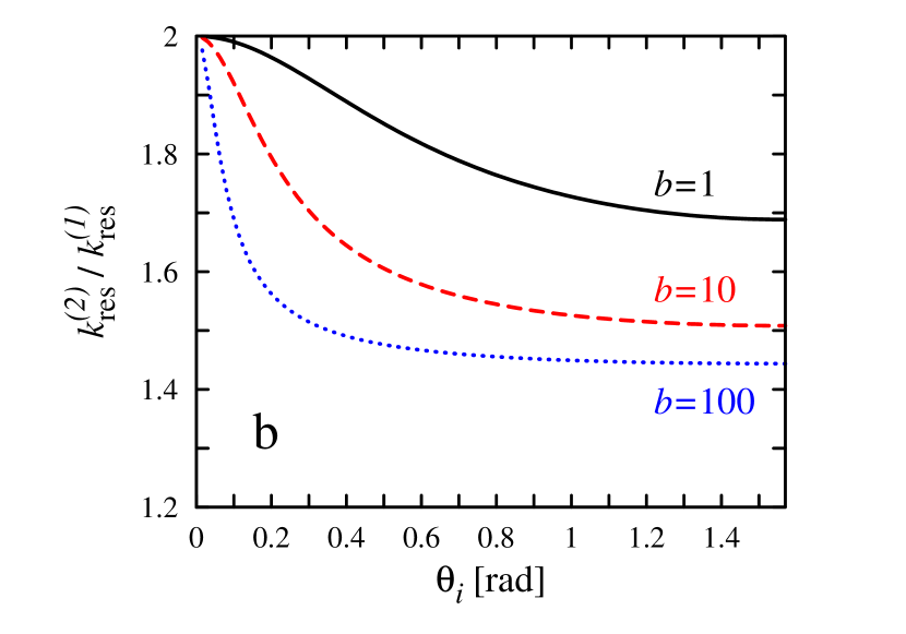
Figure 2: Dependence of the resonance position on the direction. (a) Position of the first resonance as a function of initial photon momentum direction $\theta_{i}$ for different magnetic field strength $b$. The higher the field strength, the bigger the difference between the resonant energy in various directions. (b) The ratio of the second and the first resonant energies as a function of photon momentum direction $\theta_{i}$ for various magnetic field strength $b$.

The resonances could be regularized if one takes into account the natural width of the Landau levels (Pavlov et al., 1991; Nagirner and Kiketz, 1993). The width is defined by the electron transition rates from the occupied Landau levels and depends on the magnetic field strength, the Landau level number and the electron spin state (Herold et al., 1982; Latal, 1986; Melrose and Zhelezniakov, 1981; Pavlov et al., 1991; Baring et al., 2005) (see Appendix B for detailed discussion). The spin dependence of the Landau level width is particularly important if we investigate the polarization of scattered photons. Thus, there are two widths corresponding to each Landau level - $\Gamma_{n\,s}(p_{z})$. The ground Landau level is an exceptional case. It has only one possible spin state ($s=-1$) and its width $\Gamma_{0\,-}(p_{z})=0$, since the spontaneous transition $n_{i}=0\to n_{f}=0$ is impossible with any $p_{z}$. In order to regularise the resonances one should replace the energies of the initial and the final electrons $E_{i}$ and $E_{f}$ with $E_{i}-i\Gamma_{i}/2$ and $E_{f}-i\Gamma_{f}/2$, the energy of virtual electron $E_{n}$ should be also replaced with $E_{n}+i\Gamma_{n\,s}/2$ (Pavlov et al., 1991; Nagirner and Kiketz, 1993).

Let us define the following linear combination of the width of the Landau levels:

$$\Gamma_{n}^{\pm}=\frac{\Gamma_{n\pm}}{2}+\frac{\Gamma_{i}+\Gamma_{f}}{4}.$$ (40)

Then the terms with the resonances (which we get from (32)) in the propagator could be rewritten in the regularized form. Let us also take into account the level width in the positron part. Since the positron energy is $-E_{n}$ and the level width is positive, one should change $E_{n}$ by $E_{n}-i\Gamma_{n\,s}/2$ (Graziani, 1993). Then the expression (32) can be rewritten as

$${\cal M}=\frac{v_{n+}^{+}v_{n+}^{+\dagger}}{V-E_{n}-i\Gamma_{n}^{+}}+\frac{v_{n-}^{+}v_{n-}^{+\dagger}}{V-E_{n}-i\Gamma_{n}^{-}}+\frac{v_{n+}^{-}v_{n+}^{-\dagger}}{V+E_{n}-i\Gamma_{n}^{+}}+\frac{v_{n-}^{-}v_{n-}^{-\dagger}}{V+E_{n}-i\Gamma_{n}^{-}}.$$ (41)

Useful relations for the spinor products in equation (41) are given in Appendix E.

Landau level natural width is also determines the scattering cross-section of photons with energy well below the cyclotron resonance, when $k_{i}\lesssim\Gamma_{n}$ Gonthier et al. (2014). In this case the scattering cross section saturates at small constant value for the case of photons propagating along the magnetic field direction and for the case of photons of $X$-mode polarization of any angle between the $B$-field and photon momentum (see Appendix B).

VII The S-matrix elements: phase factors

The elements of the scattering matrix are complex numbers in general and their phase factors are important in some cases: in particular it was shown by Mushtukov et al. (Mushtukov et al., 2012) that the exact form of the relativistic kinetic equation for polarized radiation demands the $S$-matrix elements and the cross section is not enough. Since we make a summation over the virtual electron Landau levels: $S_{\rm fi}=\sum_{n}S^{(n)}_{\rm fi}$, the phase factor depends on them. Nevertheless one can extract the phase factor $C_{\rm fi}$ ($S_{\rm fi}=C_{\rm fi}\sum_{n}S^{(n)}_{\rm fi}/C_{\rm fi}$) which does not depend on the variables describing the virtual electron (over which one make summation and integration in eq. (20)):

$$C_{\rm fi}=\exp\left(i\frac{(\varphi_{i}+\varphi_{f})(n_{i}-n_{f})}{2}+i\frac{(k_{{f}x}-k_{{i}x})(p_{y,i}+p_{y,f})}{2}\right).$$ (42)

The other phase factors are conjugated for a and b diagrams and depend on the virtual electron Landau level number over which the summation should be done. If we express the $S$-matrix elements with the relation $S_{\rm fi}=C_{\rm fi}\sum_{n}X^{(n)}_{\rm fi}M^{(n)}_{\rm fi}$, where $|X_{\rm fi}|=1$ and $M_{\rm fi}$ is a real number ($M_{\rm fi}\in\mathbf{R}$), then

$$X^{(n)}_{\rm fi}=\exp\left(\pm i\biggl{(}n-\frac{n_{i}+n_{f}}{2}\biggr{)}(\varphi_{f}-\varphi_{i})\mp i\frac{k_{i}k_{f}}{2}\sin\theta_{i}\sin\theta_{f}\sin(\varphi_{f}-\varphi_{i})\right).$$ (43)

Upper and lower signs correspond to the a and b Feinmann diagrams, respectively.

For the calculations of the matrix element one should know the following parameters: the quantities which define the energy and momentum of initial particles - $n_{i},\,p_{z,i}$ for the electron and $k_{i},\,\theta_{i}$ for the photon, the quantities defining the energy and momentum for the final particles - $n_{f}$ for the electron and $\theta_{f},\,(\varphi_{f}-\varphi_{f})$ for the photon. Some final quantities can be determined by the conservation laws (see Section III). The final Landau level should comply with the condition (8). It is also necessary to specify the quantities which define the polarization state of the electrons in a final and initial states - $s_{f},\,s_{i}$ and for the photon states $l_{f},\,l_{i}$. Then the recipe developed in Section V allows us to transform expression (20) and calculate the elements of the scattering matrix $S_{\rm fi}$.

The factors which are independent on the summation variable $n$ could be taken out from the summation sign. Their product is

$$-\frac{8\pi^{2}ir_{\rm e}}{\sqrt{E_{f}E_{i}}}\delta(p_{y,f}+k_{{f}y}-p_{y,i}-k_{{i}y})\delta(p_{z,f}+k_{{f}z}-p_{z,i}-k_{{i}z})\delta(E_{f}+k_{f}-E_{i}-k_{i})\frac{e^{-(|\beta_{i}|^{2}+|\beta_{f}|^{2})/4}}{4\sqrt{s_{f}s_{i}(E_{f}+s_{f})(E_{i}+s_{i})}}.$$ (44)

The obtained structure of $S$-matrix elements, which is given with (42) and (43), shows that the matrix elements are real numbers in case of scattering with only photon polarization change. It conforms to the structure of general kinetic equation for Compton scattering in strong magnetic field obtained by Mushtukov et al. (Mushtukov et al., 2012). The equation describes evolution of a density matrix kernel $\rho^{s^{\prime}}_{s}(\textbf{{k}},\textbf{{r}},t)$ (Landau and Lifshitz, 1980) and contains three items on the right hand side: $\underline{k}\,\underline{\nabla}\rho^{s^{\prime}}_{s}(\textbf{{k}},\textbf{{r}},t)=I_{1}+I_{2}+I_{3}$, where $\underline{\nabla}=(\partial/\partial t,-\nabla)$. The first two items describe photon redistribution over the polarization states only and the last term describes general photon redistribution over the energy, momentum and polarization states. It was pointed that the first term contains the elements of $S$-matrix by themselves, while the second and the third therms contain usual products of matrix elements (as a result they could be rewritten using the cross sections, which is impossible for the first term). Here we have shown that the matrix elements in the first term of the kinetic equation are real numbers and it would simplify significantly the interpretation of physics behind this term.

VIII Cross sections and redistribution function

VIII.1 Total and differential cross section

As soon as one gets the $S$-matrix elements it is possible to find the scattering cross section. The differential Compton scattering cross section for the case of fixed initial electron state is

$$\displaystyle\frac{{\rm d}\sigma}{{\rm d}\Omega_{f}}(n_{i},p_{z,i},s_{i}\,|\,k_{i},\theta_{i},l_{i},\theta_{f},l_{f},\Delta\varphi_{\rm fi})=$$

$$\displaystyle\sum\limits_{n_{f},s_{f}}\frac{E^{2}_{i}E^{2}_{f}}{(E_{i}+1)(E_{f}+1)}\frac{k_{f}}{k_{i}}\frac{\sigma_{\rm T}|S_{\rm fi}|^{2}}{(E_{i}+k_{i}-k_{f}-\cos\theta_{f}(p_{z,i}+k_{i}\cos\theta_{i}-k_{f}\cos\theta_{f}))},$$ (45)

where $\Delta\varphi_{\rm fi}=(\varphi_{i}-\varphi_{f})$. Then the total cross section is obtained from the differential cross section after the integration and summation over all possible final photon parameters:

$$\sigma_{l_{i}}(k_{i},\theta_{i};n_{i},p_{z,i},s_{i})=\frac{1}{4\pi}\sum\limits_{l_{f}}\int\limits_{0}^{\pi}{\rm d}\theta_{f}\,\sin\theta_{f}\int\limits_{0}^{2\pi}{\rm d}\varphi_{f}\frac{{\rm d}\sigma}{{\rm d}\Omega_{f}}.$$ (46)

Examples of scattering cross section on the electron at rest are given in Fig.3 for the photon which propagates along the magnetic field and in Fig.4 for the photons which propagate at some angle to the $B$-field. There is a number of resonances (38) for the case of photons which propagate angularly to the magnetic field direction, while there is only one resonance for the case of photons which propagate along the field. The difference between $X$- and $O$-mode cross sections becomes stronger as the angle between the field direction and photon momentum increases.

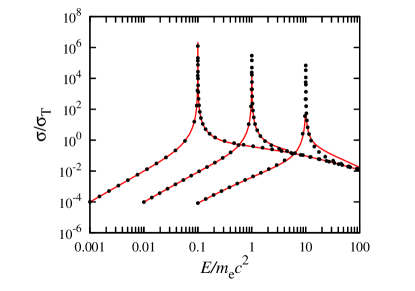
Figure 3: The exact cross-section for the photons which propagate initially along the $B$-field: $\theta_{\rm i}=0$ (red solid lines). There is no difference between polarizations in this case and only one resonance exists. Its position is defined by the field strength (39). Different curves correspond to various magnetic field strength: $b=0.1,\,1,\,10$ ($B\simeq 4.4\times 10^{12},\,\times 10^{13},\,\times 10^{14}$G). The scattering cross-section approximation obtained by Gonthier et al. (Gonthier et al., 2000) is given by black circles. It works well, but overestimates the scattering cross-section near the resonant energy and underestimates the cross section after the resonance in case of extremely high magnetic field strength: $b\gtrsim 10$.

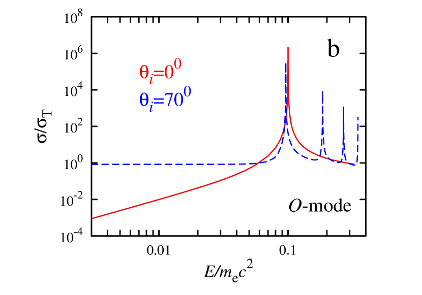
Figure 4: The cross section dependence on photon energy. (a) The cross section for the $X$- and $O$-mode photons which propagate across the magnetic field ($\theta_{i}=\pi/2$) are given by solid red and dashed blue lines correspondingly. The cross section below the first resonance shows completely different behaviour. The resonance positions are almost the same, but the cross section of the resonant scattering is also different. (b) The dependence of scattering cross section on the direction. For the case of $O$-mode photons of energies below the cyclotron energy $\sigma\propto(\sin^{2}\theta_{i}+(k/b)^{2}\cos^{2}\theta_{i})$ if $b\lesssim 1$ and $k\ll b$. Here $b=0.1$ ($B\simeq 4.4\times 10^{12}$ G).

In realistic situation, the electrons are distributed over the momentum, Landau level numbers and spin states. In a case of sufficiently strong $B$-field ($k_{\rm B}T\ll E_{\rm cycl}$) one could assume that all electrons occupy the ground Landau level and therefore take part in one-dimensional motion and have only one possible spin state ($s=-1$). In this case the differential cross section is defined by the electron distribution function $f_{n,s}(p_{z})$ (normalized as $\sum_{n,s}\int^{\infty}_{-\infty}{\rm d}p_{z}f_{n,s}(p_{z})=1$) and the cross section corresponding to the scattering by an electron with given parameters (VIII.1) is

$$\displaystyle\frac{{\rm d}\sigma^{*}}{{\rm d}\Omega_{f}}(k_{i},\theta_{i},l_{i},\theta_{f},l_{f},\Delta\varphi_{\rm fi})=\sum\limits_{n_{i},s_{i}}\int{\rm d}p_{z,i}\,\frac{{\rm d}\sigma}{{\rm d}\Omega_{f}}(n_{i},p_{z,i},s_{i}\,|\,k_{i},\theta_{i},l_{i},\theta_{f},l_{f},\Delta\varphi_{\rm fi})\,f_{n_{{i}},s_{{i}}}(p_{z,i}).$$ (47)

The total cross section in this case could be obtained from the differential one using relation (46).

Since the electrons in sufficiently strong magnetic field take part in one-dimensional motion, the cross section near the resonant energies has special features. The shape of cyclotron features depends on the direction of initial photon momentum (see Fig.5(a) and 6(a)). For the case of longitudinal propagation, the ordinary Dopple broadening takes place. For other photons, the Doppler broadening is defined by the distribution of the projection of the electron momentum. The transversal Doppler effect becomes more important as the angle between the field direction and photon momentum increases. It provides asymmetrical broadening of the cross section resonant features which is more evident for higher electron temperatures (see Fig.5(b) and 6(b)). The results of our calculations are in agreement with the previously performed calculations (Harding and Daugherty, 1991) of scattering by thermal electrons (see Fig. 7). However, a small difference in the cross section at the resonance exists because the Sokolov-Ternov wave-function are used in our calculations instead of the Johnson-Lippmann wave functions (Johnson and Lippmann, 1949) (see (Gonthier et al., 2014) for detailed discussion).

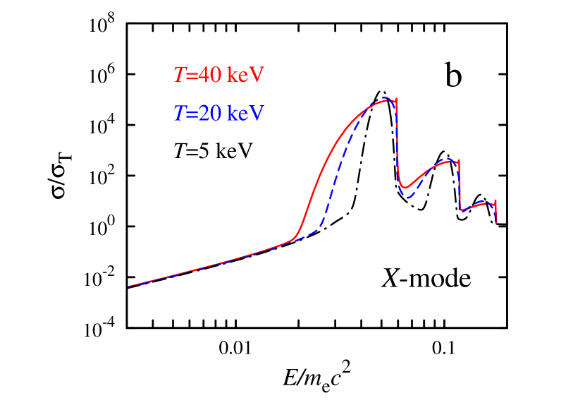
Figure 5: The cross section for the $X$-mode photons as a function of photon energy. (a) Dependence on incident angle $\theta_{i}$ for fixed electron temperature $T=20\,{\rm keV}$. (b) Dependence on electron temperature (for fixed $\theta_{i}=60^{0}$). The scattering features around the resonant energies are broadened with the width depending on the electron temperature and direction of photon momentum since the electrons mostly take part in one-dimensional motion. As a result the usual Doppler broadening takes place only for direction along the $B$-field, while in the perpendicular direction only the relativistic transversal Doppler broadening acts, and the scattering features are asymmetrical. All results are given for $b=0.05$ ($B\simeq 2.2\times 10^{12}$G).

Figure 6: Same as Fig. 5 but for the $O$-mode.

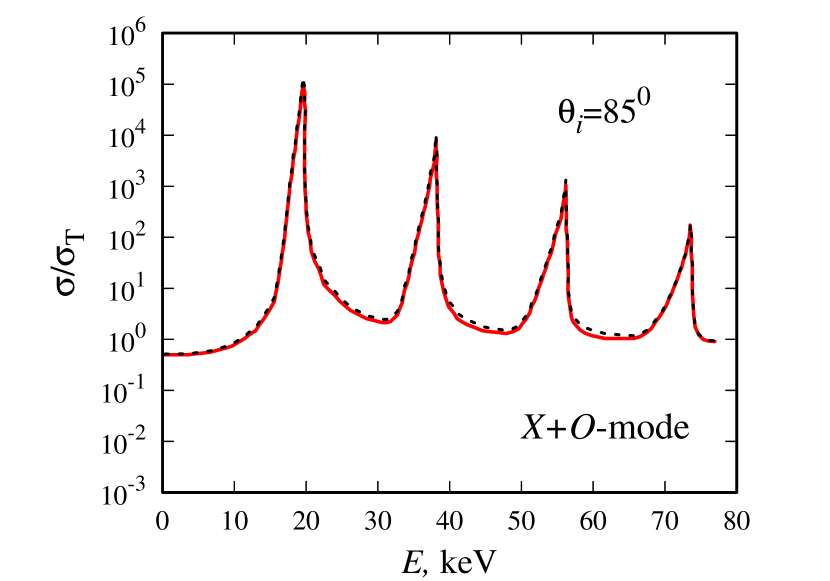
Figure 7: Polarization-averaged cross section for the case of magnetic field strength $B=1.7\times 10^{12}\,{\rm G}$, electron temperature $T=10\,{\rm keV}$ and various angles $\theta_{i}$ between the magnetic field direction and momentum of the initial photon is given by red solid lines. Black dashed line shows the results of the same calculations performed by Harding & Daugherty (Harding and Daugherty, 1991), where the Johnson-Lippmann wave functions (Johnson and Lippmann, 1949) were used.

In extremely strong magnetic field ($b>10$ or $B\gtrsim 10^{15}$ G) some interesting features take place. The resonance position and resonance energy ratios depend strongly on the direction (see Section VI) and therefore the cross section depends strongly on the direction as well (Fig. 8). It makes the problem of radiation transfer in magnetized plasma much more complicated. The dependence of resonance position on the field strength exist also for a relatively weak magnetic field, but it is not so dramatic. The resonant energies for the case of super-strong field are comparable or larger than the electron rest mass energy. As a result the decrease of relativistic cross section (“Klein-Nishina reduction”) takes place.

Figure 8: The scattering cross section as a function of initial angle between the photon momentum and magnetic field for a few initial photon energies. Since the resonant energies value depends strongly on the initial photon momentum in extremely high magnetic field, the cross section shows a strong direction dependence as well even in case of the $X$-mode polarization. Here $b=100$ ($B\simeq 4.4\times 10^{15}$G).

VIII.2 The redistribution function

In order to use the results in astrophysical applications it is useful to construct the photon redistribution function describing the Compton scattering in strong $B$-field. The set of radiation transfer equations consists of two equations, one for each polarization mode ($l=1,2$):

$$\frac{{\rm d}I_{l}(\textbf{{k}})}{{\rm d}s}=-\left(\alpha_{l}(\textbf{{k}})+\kappa_{l}(\textbf{{k}})\right)I_{l}(\textbf{{k}})+\varepsilon_{l}(\textbf{{k}})+\sum\limits_{l^{\prime}=1,2}\int\limits_{0}^{\infty}{\rm d}k^{\prime}\int\limits_{0}^{\pi}{\rm d}\theta^{\prime}\sin\theta^{\prime}\int\limits_{0}^{2\pi}{\rm d}\varphi^{\prime}R(\textbf{{k}}^{\prime},l^{\prime}\longrightarrow\textbf{{k}},l)I_{l^{\prime}}(\textbf{{k}}^{\prime}),$$ (48)

where $I_{l}(\textbf{{k}})$ is an intensity in given polarization $l$ for the photons of momentum $\textbf{{k}}=k(\sin\theta\,\cos\varphi,\sin\theta\,\sin\varphi,\cos\theta)$, $\alpha_{l}(\textbf{{k}})$ and $\kappa_{l}(\textbf{{k}})$ are absorption coefficient due to the scattering process (or scattering coefficient) and true absorption correspondingly, $\varepsilon_{l}(\textbf{{k}})$ is a true emission coefficient. The last item in the right hand side of the equation describes an emission due to the scattering processes in a given point and $R(\textbf{{k}},l\longrightarrow\textbf{{k}}^{\prime},l^{\prime})$ is the redistribution function which defines the photon probability to change the 3-momentum and the polarization state in a scattering event. The redistribution function is normalized here in the following way:

$$\sum\limits_{l^{\prime}}\int\limits_{0}^{\infty}{\rm d}k^{\prime}\int\limits_{0}^{\pi}{\rm d}\theta^{\prime}\sin\theta^{\prime}\int\limits_{0}^{2\pi}{\rm d}\varphi^{\prime}R(\textbf{{k}},l\longrightarrow\textbf{{k}}^{\prime},l^{\prime})=\alpha_{l}(\textbf{{k}}),$$ (49)

where the scattering coefficient $\alpha_{l}(\textbf{{k}})=n_{\rm e}\sigma_{l}(k,\theta)$ and $n_{\rm e}$ is an electron concentration and $\sigma_{l}(k,\theta)$ is a scattering cross section.

According to the conservation laws, there is only one or several (for each admissible final Landau levels (8)) possible final photon energies corresponding to each final photon direction in case of electron in a given quantum state, i.e. the final photon energy (7) is defined completely in case of fixed final scattering direction. The redistribution function over the zenith and azimuthal angles and polarization states is then

$$R^{*}(k_{i}|\theta_{i},\varphi_{i},l_{i}\longrightarrow\theta_{f},\varphi_{f},l_{f})\equiv\int\limits_{0}^{\infty}{\rm d}k_{f}\,R(\textbf{{k}}_{i},l_{i}\longrightarrow\textbf{{k}}_{f},l_{f})=\frac{n_{\rm e}}{4\pi}\frac{{\rm d}\sigma}{{\rm d}\Omega_{f}},$$ (50)

where the differential cross section ${{\rm d}\sigma}/{{\rm d}\Omega_{f}}$ is given by equation (VIII.1).

The general redistribution function, which corresponds to the scattering by the electron ensemble with a given distribution function over the momentum, Landau levels numbers and spin states $f_{n_{i},s_{i}}(p_{z,i})$ is:

$$R(\textbf{{k}}_{i},l_{i}\longrightarrow\textbf{{k}}_{f},l_{f})=\frac{n_{\rm e}}{4\pi}\sum\limits_{n_{i},s_{i}}\frac{{\rm d}\sigma}{{\rm d}\Omega_{f}}(n_{i},p_{z,i},s_{i}\,|\,k_{i},\theta_{i},l_{i},\theta_{f},l_{f},\Delta\varphi_{\rm fi})f_{n_{i},s_{i}}(p_{z,i})\frac{{\rm d}p_{z,i}}{{\rm d}k_{f}},$$ (51)

where the $z$-projection of electron momentum is defined by the final photon energy: $p_{z,i}=p_{z,i}(k_{f})$ and one could get it from the conservation laws (see Section III). In case of scattering by electrons in a fixed state, the electron distribution function has to be replaced with $\delta$-function. It is easy to see that the integration over the final photon energy gives us the redistribution function over the directions only (50) as it should.

The photon redistribution over the energies and momentum directions, which is given by differential cross section and redistribution function, is not trivial in general case and has to be studied carefully in each particular situation. Additional properties are caused by electron transitions between various Landau levels in a scattering event. Photon redistribution over the directions depends on the initial photon momentum direction, which is a special feature of scattering in the external field, and on the photon energy, which is typical even for the non-magnetic scattering (Klein and Nishina, 1929): the scattering indicatrix becomes more elongated in the direction of initial photon momentum as the photon energy increases. The scattering in the external magnetic field keeps this regularity but the scattering near the resonant energies adds additional features (Fig. 9) corresponding to electron transition between Landau levels: as soon as the photon energy reaches the resonant value, the ratio of forward to backward scattering cross section decrease steeply. It is potentially important for calculation of the radiation pressure resulting from a resonant Compton scattering and particularly important for constructing detailed theory of formation of a beam pattern in X-ray pulsars near the cyclotron energy.

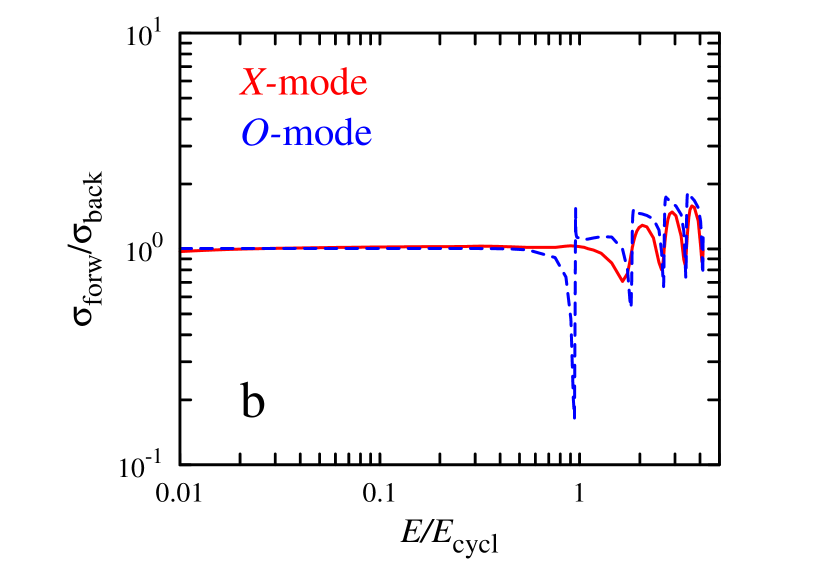
Figure 9: The ratio of forward and backward parts of the total scattering cross sections as a function of photon energy (a) for the case of photon initially propagating along ($\theta_{i}=0$) the $B$-field of different strengths and (b) across the field ($\theta_{i}=\pi/2$) of given strength $b=0.1$ ($B\simeq 4.4\times 10^{12}$G) for both photon polarizations. Sharp features appear near the resonant energies, where the electrons are able to change their Landau level. The ratio depends strongly on the initial photon momentum direction. The behaviour near the resonant energies also depends on the photon polarization.

IX Summary

Compton scattering of polarized radiation in strong magnetic field is considered. A general recipe for calculation of scattering cross section (both differential and total) and $S$-matrix elements based on second order QED perturbation theory is given as well as a recipe for calculation of photon redistribution function over photon energy, momentum and polarization. The presented scheme is adapted both for the scattering by electron with fixed momentum and for the scattering by ensemble of electrons with a given distribution over momentum. A number of calculations in our scheme were simplified analytically. As a result the discussed recipe is sufficiently easy-to-use. Because in our derivation we assume $k=|\textbf{{k}}|c$, the obtained scheme is valid up to magnetic fields of a few hundreds of the Schwinger critical value ($\sim 10^{16}$G), which covers the observed range of neutron stars magnetic field strengths including the extremely high field of magnetars. The scheme is also valid for relatively low magnetic field strength - $10^{6}-10^{9}\,{\rm G}$ - which are typical for white dwarfs, but corresponding calculations with our scheme demand large number of Landau levels which have to be taken into account. The scheme can be used in modelling the atmospheres of neutron stars, where the scattering cross section defines the opacity (Potekhin, 2014). The calculations do not assume any principal restrictions of electron momentum. It gives us a possibility to analyse directly the scattering by moving plasma, which is important for conceptions of X-ray pulsars and accreting neutron stars in general (Becker and Wolff, 2007; Poutanen et al., 2013; Serber, 2000), where Compton scattering governs plasma dynamics in the acceretion channel near the stellar surface (Basko and Sunyaev, 1975) and interaction between the radiation and matter in the accretion column for the case of bright X-ray pulsars (Mushtukov et al., 2015a; Basko and Sunyaev, 1976). Our scheme does not contain serious restrictions on the photon energy. The correct Landau level width based on the Sokolov & Ternov electron wave functions (Sokolov and Ternov, 1968, 1986) is taken into account in general case of Compton scattering for the first time, which generalizes calculations performed earlier by Gonthier et al. (Gonthier et al., 2014), which were valid for the particular case of initial photon propagating along the magnetic field and ground-to-ground state transition of the electron. The exact spin dependent width of the levels affect much the resonant scattering cross section of polarized radiation (Gonthier et al., 2014). Therefore, it has to be taken into account in models describing formation of the cyclotron features in spectra of neutron stars (Nishimura, 2008; Ferrigno et al., 2011).

We have discussed separately the elements of the scattering matrix, which are important for solution of exact relativistic kinetic equation for Compton scattering in a strong $B$-field obtained in our resent work (Mushtukov et al., 2012). It was shown that the $S$-matrix element are real numbers in case when they describe scattering with polarisation changes only.

Potentially important astrophysical results arise from the behaviour of resonant scattering. The resonance position depends on the direction. The stronger the $B$-field, the stronger the dependence (see Fig. 2 left). The position of the fundamental varies by $\approx 20\,\%$ for $B\sim 10^{13}\,{\rm G}$ and even more for higher field strength. It can be used in diagnostics of X-ray pulsars since this effect would partly define the changes of the cyclotron absorption line position during the pulse period (Lutovinov et al., 2015). The ratio of the energies of first and second resonances $k_{\rm res}^{(2)}/k_{\rm res}^{(1)}$ is also depend on the direction in a strong magnetic field (see Fig. 2 right), and it can cause the change of the ratio of cyclotron line energies during pulse period (Lutovinov et al., 2015) and nonequidistance of the cyclotron line harmonics, which was observed in spectra of X-ray pulsars (Tsygankov et al., 2006). The effect is also causes the variations of scattering cross section with the angle even for the case of $X$-mode photons (see Fig. 8). It is particularly important for radiation transfer and radiation pressure calculation in case of high $B$-field, since the opacity would strongly depend on directions. It was pointed that the photon redistribution over directions changes as soon as the initial photon energy crosses the resonant value (see Fig. 9). It is potentially important for the formation of a beam pattern of X-ray pulsars near the cyclotron line.

The presented scheme of calculation provides a ground for investigation of radiation transfer in strongly magnetised plasma. It can be readily applied to astrophysical problems, principally for the models of spectrum formation in strongly magnetized neutron stars, calculation of radiation pressure in strong $B$-field and modelling of X-ray pulsar beam pattern all over the spectrum. In this way, the presented scheme is extremely relevant to further investigation of strongly magnetized neutron stars.

Appendix A Longitudinal transformation of electron and photon momenta

We are focusing here on the longitudinal Lorentz transformation of the timelike component of the 4-momentum $p_{0}$, i.e. particle’s energy, and the $z$-component of the momentum $p_{z}$, which corresponds to the particle momentum along the magnetic field. The general form of the longitudinal transformation is

$$p_{0}^{\prime}=(p_{0}-\beta\,p_{z})/\sqrt{1-\beta^{2}},\quad p^{\prime}_{z}=(p_{z}-\beta\,p_{0})/\sqrt{1-\beta^{2}},$$ (52)

where $\beta$ is the velocity between the reference frames along the magnetic field in units of speed of light. The transformation (52) can be rewritten in another form using parameter $\chi$, which satisfies the relation $\beta=\tanh\chi$. Then

$$p_{0}^{\prime}=p_{0}\cosh\chi-p_{z}\sinh\chi,\quad p_{z}^{\prime}=p_{z}\cosh\chi-p_{0}\sinh\chi.$$ (53)

Thus the photon energy and the longitudinal momentum are transformed as follows:

$$k^{\prime}=k(\cosh\chi-\sinh\chi\cos\theta),\quad k^{\prime}\cos\theta^{\prime}=k(\cos\theta\cosh\chi-\sinh\chi).$$ (54)

The transformation of the angle between the $B$-field direction and the photon momentum is given by the relations

$$\cos\theta^{\prime}=\frac{\cos\theta\cosh\chi-\sinh\chi}{\cosh\chi-\sinh\chi\cos\theta},\,\,\sin\theta^{\prime}=\frac{\sin\theta}{\cosh\chi-\sinh\chi\cos\theta}.$$ (55)

The electron energy $E_{n}$ and momentum along the magnetic field $p_{z}$ are transformed according to (52):

$$E^{\prime}_{n}=E_{n}\cosh\chi-p_{z}\sinh\chi,\quad p_{z}^{\prime}=p_{z}\cosh\chi-E_{n}\sinh\chi.$$ (56)

Using relation ${\rm d}E_{n}=p_{z}{\rm d}p_{z}/E_{n}$ we get:

$${\rm d}p_{z}^{\prime}={\rm d}p_{z}\cosh\chi-{\rm d}E_{n}\sinh\chi=\left(\cosh\chi-\frac{p_{z}}{E_{n}}\sinh\chi\right){\rm d}p_{z}=\frac{{\rm d}p_{z}}{E_{n}}(E_{n}\cosh\chi-p_{z}\sinh\chi)=\frac{E_{n}^{\prime}}{E_{n}}{\rm d}p_{z}.$$ (57)

Therefore the ratio ${{\rm d}p_{z}}/{E_{n}}$ is conserved under longitudinal Lorentz transformation.

If photon energy $k$ and momentum along the field $k_{z}$ are given at the laboratory reference frame, where the electron momentum along the field is $p_{z}$, then the photon energy $k^{\prime}$ and momentum $k^{\prime}_{z}$ in the electron reference frame (where $p_{z}=0$) are

$$k^{\prime}=\frac{k}{\sqrt{E_{n}^{2}-p_{z}^{2}}}(E_{n}-p_{z}\cos\theta),\quad k_{z}^{\prime}=\frac{k}{\sqrt{E_{n}^{2}-p_{z}^{2}}}(E_{n}\cos\theta-p_{z}).$$ (58)

The angle $\theta^{\prime}$ between the photon momentum and magnetic field direction satisfies following relations:

$$\cos\theta^{\prime}=\frac{E_{n}\cos\theta-p_{z}}{E_{n}-p_{z}\cos\theta},\quad\sin\theta^{\prime}=\frac{\sqrt{E_{n}^{2}-p_{z}^{2}}\sin\theta}{E_{n}-p_{z}\cos\theta}.$$ (59)

Appendix B Landau level natural width

Landau level natural width for the particular case of $p_{z,i}=0$ is defined as a sum of the partial widths:

$$\Gamma_{n}^{\pm}=\sum\limits_{n^{\prime}<n}\Gamma_{nn^{\prime}}^{\pm}.$$ (60)

The general expression for the partial width was obtained by Herold et al. (Herold et al., 1982) for transition between arbitrary Landau levels but for zero initial electron momentum $p_{z,i}=0$:

$$\displaystyle\Gamma_{nn^{\prime}}^{\pm}=\frac{r_{\rm e}}{2}\int\limits_{0}^{\pi/2}{\rm d}\theta\frac{k\sin\theta}{E_{n}\sqrt{E^{2}_{n}-2(n-n^{\prime})b\sin^{2}\theta}}$$

$$\displaystyle\times\left\{\left[(E_{n}\mp 1)(E_{n}\pm 1-k)I^{2}_{n,n^{\prime}}(u)+(E_{n}\pm 1)(E_{n}\mp 1-k)I^{2}_{n-1,n^{\prime}-1}(u)\right]\sin^{2}\theta\right.$$

$$\displaystyle+\left[(E_{n}\pm 1)(E_{n}\mp 1-k)I^{2}_{n-1,n^{\prime}}(u)+(E_{n}\mp 1)(E_{n}\pm 1-k)I^{2}_{n,n^{\prime}-1}(u)\right](1+\cos^{2}\theta)$$

$$\displaystyle+2k\sqrt{2nb}\left[I^{2}_{n,n^{\prime}}(u)I^{2}_{n-1,n^{\prime}}(u)+I^{2}_{n,n^{\prime}-1}(u)I^{2}_{n-1,n^{\prime}-1}(u)\right]\sin\theta\cos^{2}\theta$$

$$\displaystyle+\left.4b\sqrt{nn^{\prime}}\left[I^{2}_{n-1,n^{\prime}}(u)I^{2}_{n,n^{\prime}-1}(u)+I^{2}_{n,n^{\prime}}(u)I^{2}_{n-1,n^{\prime}-1}(u)\right]\sin^{2}\theta\right\},$$ (61)

where $E_{n}=\sqrt{1+2nb}$ is the electron energy, $k=\left[E_{n}-(E^{2}_{n}-2(n-n^{\prime})b\sin^{2}\theta)^{1/2}\right]/\sin^{2}\theta$ is the energy of a photon emitted at the angle $\theta$ due to the electron transition $n\longrightarrow n^{\prime}$,

$$I_{n,n^{\prime}}(u)=(-1)^{n}(n!n^{\prime}!)^{-1/2}\exp[u/2]u^{(n-n^{\prime})/2}\frac{\partial^{n}}{\partial u^{n}}\left(u^{n^{\prime}}\exp[-u]\right)$$ (62)

and $u=(k^{2}\sin^{2}\theta)/2b$ (Canuto and Ventura, 1977). The functions $I_{n,n^{\prime}}(u)$ can be constructed using the associated Laguerre polynomials $L_{n}^{\alpha}(x)$:

$$I_{n,n^{\prime}}(u)=(-1)^{n}(n!/n^{\prime}!)^{1/2}\exp[-u/2]u^{(n^{\prime}-n)/2}L_{n}^{n^{\prime}-n}(u),\quad L_{n}^{\alpha}(x)\equiv\frac{e^{x}x^{-\alpha}}{n!}\frac{{\rm d}^{n}}{{\rm d}x^{n}}\left[e^{-x}x^{n+\alpha}\right].$$ (63)

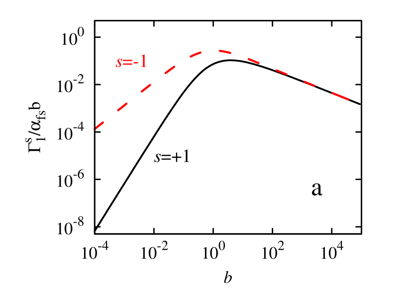
Figure 10: Spin dependent Landau level width in the electron rest frame (in units of $\alpha_{\rm fs}b$) as a function of dimensionless magnetic field strength $b=B/B_{\rm cr}$ is given for the first Landau level (a) and for the 1st, 5th and 25th Landau levels of spin state $s=-1$ (b).

Compact approximate expressions for $\Gamma^{\pm}_{n}$ and $\Gamma^{\pm}_{nn^{\prime}}$ for the particular cases of $nb\ll 1$ (non-relativistic limit), $b^{-1}\ll n\ll b^{-3}$ (ultrarelativistic quasi-classical limit) and $n\gg b^{-3}$ (ultrarelativistic quantum limit) were provided by Pavlov et al. (Pavlov et al., 1991). The Landau level widths for the case of nonzero momentum of the electron along the field $p_{z,i}\neq 0$ can be obtained from those expressions for $p_{z,i}=0$ by Lorentz transformation (Herold et al., 1982): $\Gamma_{n}^{\pm}(p_{z})=\Gamma_{n}^{\pm}\sqrt{1+2bn}/E_{n}(p_{z})$.

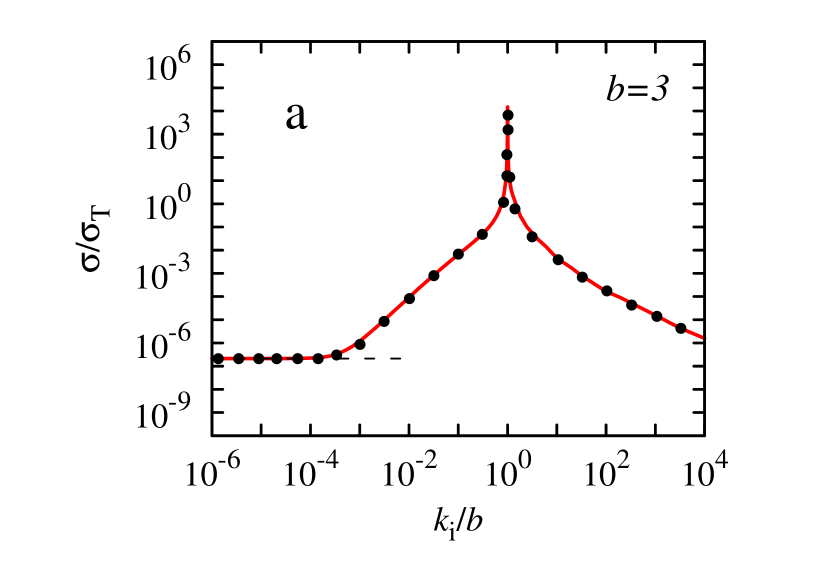
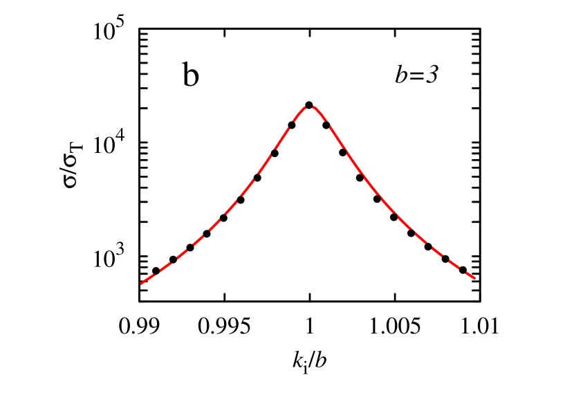
Figure 11: Compton scattering cross section calculated using spin-dependent Landau level width for the particular case of ground-to-ground state transition is given by the red solid lines in a wide photon energy range (a) and for photon of energy close to the fundamental (b). The magnetic field strength $b=B/B_{\rm cr}=3$ and initial angle between the field direction and photon momentum $\theta_{i}=0$. Black dots represent calculations performed by Gonthier et al. (Gonthier et al., 2014) for the same conditions. The Landau level width affects strongly the cross section at low energies, where the level width becomes comparable to the photon energy and the cross section saturates at a small constant value (64) given by the black dashed line (a). The level width also affects strongly the cross section at the resonance energies (b).

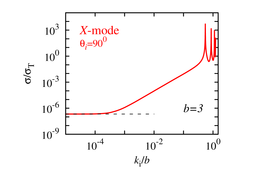
Figure 12: Scattering cross section for the $X$-mode photons of initial angle $\theta_{i}=90^{\circ}$ in a wide range of initial photon energies. The magnetic field strength $b=B/B_{\rm cr}=3$. At low energies the cross section saturates at a small constant value (64) given by the black dashed line similarly to the case of photons propagating along the $B$-field (see Fig. 11a).

Cyclotron decay rates for transition to the ground state and arbitrary initial electron momentum $p_{z,i}$ were obtained by Latal (Latal, 1986). The simplified expressions were introduces by Baring et al. (Baring et al., 2005). Although the resonance line widths involve infinite sums over Landau levels, in the case of fundamental resonance the sum is dominated by the $n=1$ state. The width of this state is equal to the $n\longrightarrow 0$ cyclotron decay rate. As a result, the fundamental line width can be well approximated by the particular cyclotron rate obtained by Latal (Latal, 1986; Baring et al., 2005). For the case of $b\gg 1$ cyclotron transitions to the ground Landau level dominate (Harding and Preece, 1987) and the cyclotron decay rate for $n\longrightarrow 0$ transitions approximate well the widths of excited states.

Landau level natural width becomes crucially important at resonant photon energies (see Section VI) and at energies well below the cyclotron energy, when the initial photon energy becomes comparable to the Landau level width (Gonthier et al., 2014). If $k_{i}\ll\Gamma$ the cross section for the photons propagating along the magnetic field saturates at a small value

$$\sigma\approx\sigma_{\rm T}\Gamma^{2}b^{-2}(1+2b)^{-1}.$$ (64)

The same happens with photons of $X$-mode propagating in any direction (see Fig. 12).

Appendix C Set of used matrices and useful relations

In this section we present the matrices which we use in our calculations. In general we are following the standard designations (Bogoli’ubov and Shirkov, 1959; Berestetskii et al., 1971; Peskin and Schroeder, 1995).

We use a set of three $2\times 2$ Pauli matrices, $\sigma_{1},\,\sigma_{2},$ and $\sigma_{3}$, which are Hermitian and unitary, in their standard designation (Peskin and Schroeder, 1995). $I$ is a unity $2\times 2$ matrix. We also use the following combinations of Pauli matrices: $\sigma^{\pm}=(I\pm\sigma_{3})/2,\,\,\,\sigma_{\pm}=(\sigma_{1}\pm i\,\sigma_{2})/2.$

The gamma (Dirac) matrices which compose the 4-dimensional vector $\underline{\gamma}=\{\gamma^{0},\gamma^{1},\gamma^{2},\gamma^{3}\}$ could be expressed via the $2\times 2$ Pauli matrices:

$$\gamma^{0}=\gamma_{0}=\left(\begin{array}[]{cc}I&0\\ 0&-I\end{array}\right),\,\,\,\gamma^{i}=-\gamma_{i}=\left(\begin{array}[]{cc}0&\sigma_{i}\\ -\sigma_{i}&0\end{array}\right).$$ (65)

We also introduce matrices $\underline{D}=\{D^{0},\textbf{D}\}$, where:

$$D^{0}=\left(\begin{array}[]{cc}0&-I\\ I&0\end{array}\right),\,\,\,D^{i}=\left(\begin{array}[]{cc}-\sigma_{i}&0\\ 0&\sigma_{i}\end{array}\right),$$ (66)

and 3-dimensional vectors of matrices $\boldsymbol{\alpha}$ and $\boldsymbol{\Sigma}$:

$$\alpha_{i}=\left(\begin{array}[]{cc}0&\sigma_{i}\\ \sigma_{i}&0\end{array}\right),\,\,\,\Sigma_{i}=\left(\begin{array}[]{cc}\sigma_{i}&0\\ 0&\sigma_{i}\end{array}\right).$$ (67)

Let us designate the unity matrix $4\times 4$ with 1, and the product of four matrices with $\gamma_{5}$:

$$\gamma_{5}=-\gamma^{5}=i\,\gamma^{0}\,\gamma^{1}\,\gamma^{2}\,\gamma^{3}=\left(\begin{array}[]{cc}0&I\\ I&0\end{array}\right).$$ (68)

We also use the following linear combination of the matrices:

$$\Sigma^{\pm}=(I\pm\Sigma_{3})/2,\,\,\Sigma_{\pm}=(\Sigma_{1}\pm i\,\Sigma_{2})/2,\,\,\alpha^{\pm}=(\gamma_{5}\pm\alpha_{3})/2,\,\,\alpha_{\pm}=(\alpha_{1}\pm i\,\alpha_{2})/2,$$ (69)

$$D^{\pm}=(\gamma^{0}\mp D^{3})/2,\,D_{\pm}=-(D^{1}\pm i\,D^{2})/2,\,\gamma^{\pm}=(-D^{0}\pm\gamma^{3})/2,\,\gamma_{\pm}=(\gamma^{1}\pm i\,\gamma^{2})/2.$$ (70)

These matrices compose the set of 16 linearly independent $4\times 4$ matrices. They could be expressed via $2\times 2$ matrices in the following way:

$$\Sigma^{\pm}=\left(\begin{array}[]{cc}\sigma^{\pm}&0\\ 0&\sigma^{\pm}\end{array}\right),\,\,\,\Sigma_{\pm}=\left(\begin{array}[]{cc}\sigma_{\pm}&0\\ 0&\sigma_{\pm}\end{array}\right),\,\,\,\alpha^{\pm}=\left(\begin{array}[]{cc}0&\sigma^{\pm}\\ \sigma^{\pm}&0\end{array}\right),\,\,\,\alpha_{\pm}=\left(\begin{array}[]{cc}0&\sigma_{\pm}\\ \sigma_{\pm}&0\end{array}\right),$$ (79)

$$D^{\pm}=\left(\begin{array}[]{cc}\sigma^{\pm}&0\\ 0&-\sigma^{\pm}\end{array}\right),\,\,\,D_{\pm}=\left(\begin{array}[]{cc}\sigma_{\pm}&0\\ 0&-\sigma_{\pm}\end{array}\right),\,\,\,\gamma^{\pm}=\left(\begin{array}[]{cc}0&\sigma^{\pm}\\ -\sigma^{\pm}&0\end{array}\right),\,\,\,\gamma_{\pm}=\left(\begin{array}[]{cc}0&\sigma_{\pm}\\ -\sigma_{\pm}&0\end{array}\right).$$ (88)

The Dirac matrices are determined by relations of anticommutativity. For the 4-vectors of matrices they are

$$\gamma^{\mu}\gamma^{\nu}+\gamma^{\nu}\gamma^{\mu}=2g^{\mu\nu},\quad\gamma_{5}\underline{\gamma}+\underline{\gamma}\gamma_{5}=0,\quad D^{\mu}D^{\nu}+D^{\nu}D^{\mu}=-2g_{\mu\nu},\quad\gamma_{5}\underline{D}+\underline{D}\gamma_{5}=0,$$ (89)

and for the 3-vectors of matrices the relations are

$$\alpha_{k}\alpha_{j}+\alpha_{j}\alpha_{k}=2\delta_{kj},\quad\Sigma_{k}\Sigma_{j}+\Sigma_{j}\Sigma_{k}=2\delta_{kj},\quad D^{k}\Sigma_{j}+\Sigma_{j}D^{k}=-2\gamma^{0}\delta_{kj}.$$ (90)

Useful commutative relations are:

$$D^{\mu}\gamma^{\nu}-\gamma^{\nu}D^{\mu}=2\gamma_{5}g^{\mu\nu},\quad\gamma^{k}\alpha_{j}-\alpha_{j}\gamma^{k}=2\gamma^{0}\delta_{kj}.$$ (91)

The useful dot products of the 4-vectors ($\underline{a}\,\underline{b}\equiv a^{0}b^{0}-\sum_{i=1}^{3}a^{i}b^{i}$) of matrices are

$$\underline{\gamma}\,\underline{\gamma}=4,\quad\underline{D}\,\underline{D}=-4,\quad\underline{\gamma}\underline{D}=-\underline{D}\underline{\gamma}=-4\gamma_{5}$$ (92)

and for the 3-vectors ($\textbf{ab}\equiv\sum_{i=1}^{3}a^{i}b^{i}$) of matrices are

$$\boldsymbol{\gamma}\boldsymbol{\gamma}=-3,\quad\boldsymbol{\gamma}\boldsymbol{\alpha}=-\boldsymbol{\alpha}\boldsymbol{\gamma}=3\gamma^{0},\quad\boldsymbol{\gamma}\boldsymbol{\Sigma}=\boldsymbol{\Sigma}\boldsymbol{\gamma}=-3D^{0},\quad\boldsymbol{\gamma}\textbf{D}=-\textbf{D}\boldsymbol{\gamma}=3\gamma_{5},$$ (93)

$$\boldsymbol{\alpha}\boldsymbol{\alpha}=3,\quad\boldsymbol{\alpha}\boldsymbol{\Sigma}=\boldsymbol{\Sigma}\boldsymbol{\alpha}=3\gamma^{0},\quad\boldsymbol{\alpha}\textbf{D}=-\textbf{D}\boldsymbol{\alpha}=-3D^{0},$$ (94)

$$\boldsymbol{\Sigma}\boldsymbol{\Sigma}=3,\quad\textbf{D}\textbf{D}=3,\quad\boldsymbol{\Sigma}\textbf{D}=\textbf{D}\boldsymbol{\Sigma}=3\gamma^{0}.$$ (95)

Appendix D Electron in the external magnetic field

In this section we discuss the description of an electron in the external magnetic field which we use in this paper. The different ways of electron description in such case are also discussed in literature (Sokolov and Ternov, 1986; Herold et al., 1982; Mészáros, 1992).

D.1 Dirac equation

The electron is described by the Dirac equation, which has to be written for the case of external magnetic field. Let us choose 4-vector of potential in the Landau gauge: $\underline{A}_{\rm e}=\{0,{\bf{A}}_{\rm e}\}$, where ${\bf{A}}_{\rm e}=B_{\rm e}\,(0,x,0)$. Then the required solutions $\Psi$ satisfy the equation:

$$\left(\hat{p}+\frac{e}{c}\hat{A}_{\rm e}-m\,c\right)\,\Psi=0,$$ (96)

where $\hat{A}_{\rm e}=\underline{A}_{\rm e}\underline{\gamma}=-B_{\rm e}\,x\gamma^{2}$, $\gamma^{2}$ is one of the Pauli matrices (65) and $\hat{p}=\underline{p}\,\underline{\gamma}=i\,\hbar\,\underline{\nabla}\underline{\gamma}$.

Let us use relativistic quantum system of units and find the solution in the following form: $\Psi=\exp{[i(-Et+p_{z}z+p_{y}y)]}\,\psi$. It is useful to change the variables: $x=u-p_{y}/b$. Then Dirac equation (96) takes form

$$\left(E\,\gamma^{0}+i\,\frac{{\rm d}}{{\rm d}u}\gamma^{1}-p_{z}\,\gamma^{3}-b\,u\gamma^{2}-1\right)\,\psi(u)=0.$$ (97)

If it is multiplied by $i\gamma^{1}$, then we get the ordinary system of differential equations:

$$\left(\frac{{\rm d}}{{\rm d}u}-i\,E\,\alpha_{1}-b\,u\,\Sigma_{3}+p_{z}\,\Sigma_{2}-i\,\gamma^{1}\right)\,\psi(u)=0.$$ (98)

D.2 From the system of equations to second order differential equations

Let designate the components of the vector which we want to find: $\psi(u)=(\psi_{1},\psi_{2},\psi_{3},\psi_{4})^{\rm T}$, and rewrite the ordinary system of differential equations (98) in details:

$$\left\{\begin{array}[]{lllll}\displaystyle{{\rm d}\psi_{1}}/{{\rm d}u}=bu\psi_{1}+p_{z}i\psi_{2}+0+i(E+1)\psi_{4}\\ \displaystyle{{\rm d}\psi_{2}}/{{\rm d}u}=-p_{z}i\psi_{1}-bu\psi_{2}+i(E+1)\psi_{3}+0\\ \displaystyle{{\rm d}\psi_{3}}/{{\rm d}u}=0+i(E-1)\psi_{2}+bu\psi_{3}+p_{z}i\psi_{4}\\ \displaystyle{{\rm d}\psi_{4}}/{{\rm d}u}=i(E-1)\psi_{1}+0-p_{z}i\psi_{3}-bu\psi_{4}\end{array}\right..$$ (99)

Then we can find equations for each function in (99):

1) The case of $\psi_{1}=0$ gives an equation for $\psi_{3}$. Using the designations: $\zeta\equiv(E+1)\psi_{3}$ and $a\equiv E^{2}-1-p_{z}^{2}$, we get: $\psi_{1}=0,\quad p_{z}\psi_{2}+(E+1)\psi_{4}=0,\quad\psi_{2}^{\prime}=-bu\psi_{2}+i\zeta,\quad\zeta^{\prime}=ia\psi_{2}+bu\zeta.$ Therefore:

$$\zeta^{\prime\prime}=(b^{2}u^{2}+b-a)\zeta.$$ (100)

2) The case of $\psi_{2}=0$ gives a solution for $\psi_{4}$. Defining $\mu\equiv(E+1)\psi_{4}$, we get $\psi_{2}=0$, $-p_{z}\psi_{1}+(E+1)\psi_{3}=0$, $\psi_{1}^{\prime}=bu\psi_{1}+i\mu$, $\mu^{\prime}=ia\psi_{1}-bu\mu$. Therefore:

$$\mu^{\prime\prime}=(b^{2}u^{2}-b-a)\mu.$$ (101)

3) The case of $\psi_{3}=0$ gives us a solution for $\psi_{1}$. Defining $\eta\equiv(E-1)\psi_{1}$, we get $\psi_{3}=0$, $(E-1)\psi_{2}+p_{z}\psi_{4}=0$, $\psi_{4}^{\prime}=-bu\psi_{4}+i\eta$, $\eta^{\prime}=ia\psi_{4}+bu\eta$. Here we get the same equation as in a first case (100): $\eta^{\prime\prime}=(b^{2}u^{2}+b-a)\eta.$

4) The case of $\psi_{4}=0$ gives us a solution for $\psi_{2}$. Defining $\kappa\equiv(E-1)\psi_{2}$ and using similar designations as in the second case we get $\psi_{4}=0$, $(E-1)\psi_{1}-Z\psi_{3}=0$, $\psi_{3}^{\prime}=bu\psi_{3}+i\kappa$, $\kappa^{\prime}=ia\psi_{3}-bu\kappa$. And we get the same equation as in a second case: $\kappa^{\prime\prime}=(b^{2}u^{2}-b-a)\kappa$.

Thus the system of equations (99) is reduced to the pair of equations of the same form: (100) and (101). Both of them can be transformed to the equation of quantum harmonic oscillator. Its solutions are well known and enumerated with integer numbers $n\geq 0$:

$$\frac{1}{2}\left[-{\frac{{\rm d}^{2}\phi_{n}(\xi)}{{\rm d}\xi^{2}}}+\xi^{2}\phi_{n}(\xi)\right]=\left(n+\frac{1}{2}\right)\phi_{n}(\xi).$$ (102)

The eigen functions could be written via the Hermite polynomials: $\phi_{n}(\xi)=\pi^{-1/4}(2^{n}n!)^{-1/2}e^{-\xi^{2}/2}H_{n}(\xi)$. Thus, we find that the motion of electrons is quantized and they occupy Landau levels.

The eigen functions form orthonormalized series. The expressions for the derivative take the form:

$$\phi_{n}^{\prime}(\xi)=\sqrt{2n}\phi_{n-1}(\xi)-\xi\phi_{n}(\xi),\,\,\phi_{n-1}^{\prime}(\xi)=-\sqrt{2n}\phi_{n}(\xi)+\xi\phi_{n-1}(\xi).$$

Our solutions will be expressed through the functions $\chi_{n}(u)$, which are defined by harmonic oscillator eigen functions $\phi_{n}(\xi)$ and comply with the relations:

$$\displaystyle\chi_{n}(u)=b^{1/4}i^{n}\phi_{n}(b^{1/2}u),\,\,\frac{1}{2}\left[-\frac{1}{b}\frac{{\rm d}^{2}\chi_{n}(\xi)}{{\rm d}\xi^{2}}+b\xi^{2}\chi_{n}(\xi)\right]=\left(n+\frac{1}{2}\right)\chi_{n}(\xi),$$ (103)

$$\displaystyle\chi_{n}^{\prime}(u)=ib_{n}\chi_{n-1}(u)-bu\chi_{n}(u),\,\,\chi_{n-1}^{\prime}(u)=ib_{n}\chi_{n}(u)+bu\chi_{n-1}(u),\,\,b_{n}=\sqrt{2bn}.$$ (104)

Functions $\chi_{n}(u)$ are normalized: $\int_{-\infty}^{\infty}\chi^{*}_{n}(\xi)\chi_{n^{\prime}}(\xi){\rm d}\xi=\delta_{nn^{\prime}}$.

D.3 Solution of the system of equations

The solutions of the second order equations (100,101) give us a solution of the system of the equations (99). Let us enumerate the solutions with the upper index $(l)$ and gather them into the matrix $\left(\psi_{j}^{(l)}(u)\right)$:

$$\psi=\left(\psi_{j}^{(l)}(u)\right)=\left(\begin{array}[]{cccc}(E+1)\chi_{n-1}&0&p_{z}\chi_{n-1}&b_{n}\chi_{n-1}\\ 0&(E+1)\chi_{n}&b_{n}\chi_{n}&-p_{z}\chi_{n}\\ p_{z}\chi_{n-1}&b_{n}\chi_{n-1}&(E-1)\chi_{n-1}&0\\ b_{n}\chi_{n}&-p_{z}\chi_{n}&0&(E-1)\chi_{n}\end{array}\right).$$ (105)

However, these solutions are linearly dependent: $(E-1)\psi^{(1)}=p_{z}\psi^{(3)}+b_{n}\psi^{(4)}$, $(E-1)\psi^{(2)}=b_{n}\psi^{(3)}-p_{z}\psi^{(4)}$. In order to get four independent solutions one have to use the ones with the negative energy $E=\pm E_{n}$, $E_{n}=\sqrt{1+b_{n}^{2}+p_{z}^{2}}$, which correspond to the positrons. Let us write down the solutions. Two of them correspond to the electrons and have the form:

$$\Psi_{nj}^{+}(x,y,z,p_{y},p_{z})=\left(\frac{E_{n}+1}{2E_{n}}\right)^{1/2}v_{nj}^{+}(p_{z},u)e^{-i(E_{n}t-p_{y}y-p_{z}z)},\,\,j=1,2,$$ (106)

where

$$v_{n1}^{+}(p_{z},u)=\left(\begin{array}[]{c}\chi_{n-1}(u)\\ 0\\ p_{z}\chi_{n-1}(u)/(E_{n}+1)\\ b_{n}\chi_{n}(u)/(E_{n}+1)\end{array}\right),\qquad v_{n2}^{+}(p_{z},u)=\left(\begin{array}[]{c}0\\ \chi_{n}(u)\\ b_{n}\chi_{n-1}(u)/(E_{n}+1)\\ -p_{z}\chi_{n}(u)/(E_{n}+1)\end{array}\right).$$

And two of them correspond to the positron states:

$$\Psi_{nj}^{-}(x,y,z,p_{y},p_{z})=\left(\frac{E_{n}+1}{2E_{n}}\right)^{1/2}v_{nj}^{-}(p_{z},u)e^{i(E_{n}t+p_{y}y+p_{z}z)},\,\,j=1,2,$$ (107)

where

$$v_{n1}^{-}(p_{z},u)=\left(\begin{array}[]{c}-p_{z}\chi_{n-1}(u)/(E_{n}+1)\\ -b_{n}\chi_{n}(u)/(E_{n}+1)\\ \chi_{n-1}(u)\\ 0\end{array}\right),\qquad v_{n2}^{-}(p_{z},u)=\left(\begin{array}[]{c}-b_{n}\chi_{n-1}(u)/(E_{n}+1)\\ p_{z}\chi_{n}(u)/(E_{n}+1)\\ 0\\ \chi_{n}(u)\end{array}\right)$$

and $u=x+p_{y}/b$.

The wave functions could be also presented in the following form:

$$\Psi_{nj}^{-}(x,y,z,-p_{y},-p_{z})=\left(\frac{E_{n}+1}{2E_{n}}\right)^{1/2}v_{ns}^{-}(-p_{z},u)e^{i(E_{n}t-p_{y}y-p_{z}z)},\,\,s=1,2,$$ (108)

where $u=x-p_{y}/b$. In case of $n=0$ two solutions vanish: $v_{01}^{+}(p_{z},u)=v_{01}^{-}(p_{z},u)=0$.

D.4 The solutions for definite helicity

Let as find now the solutions in a form when they are eigenvectors of the helicity operators $\tilde{S}$ and $\mu$ (non self-conjugated and self-conjugated correspondingly) (Bogoli’ubov and Shirkov, 1959). They would be the linear combinations of the solutions with indexes $s=1,2$. The helicity operator $\tilde{S}$ acts on the 4-vectors only and it does not act on the functions $\chi$. Therefore these functions are multiplier factors in front of the eigenvectors of the operator $\tilde{S}$:

$$U_{1}(p_{z})=\left(\begin{array}[]{c}E_{n}+s_{n}\\ 0\\ p_{z}\\ 0\end{array}\right),\quad U_{2}(p_{z})=\left(\begin{array}[]{c}0\\ E_{n}+s_{n}\\ 0\\ -p_{z}\end{array}\right),\quad U_{3}(p_{z})=\left(\begin{array}[]{c}p_{z}\\ 0\\ E_{n}+s_{n}\\ 0\end{array}\right),\quad U_{4}(p_{z})=\left(\begin{array}[]{c}0\\ -p_{z}\\ 0\\ E_{n}+s_{n}\end{array}\right),$$ (109)

where $E_{n}=\sqrt{1+2nb+p_{z}^{2}}$ is the particle energy and $s_{n}=\sqrt{1+2bn}$. Thus it is necessary to consider four linear combinations.

1) For the electron with the helicity $+1$ the following relation could be written down:

$$C_{1}v^{+}_{n1}(p_{z},u)+C_{2}v^{+}_{n2}(p_{z},u)=v_{n+}^{+}(p_{z},u)=\alpha_{1}U_{1}\chi_{n-1}+\alpha_{2}U_{4}\chi_{n}.$$

And therefore one finds out the relations for the coefficients:

$$\displaystyle C_{1}=\alpha_{1}\sqrt{\frac{E_{n}+s_{n}}{2s_{n}}},\quad C_{2}=-\alpha_{2}\frac{p_{z}}{\sqrt{2s_{n}(E_{n}+s_{n})}},$$

$$\displaystyle C_{1}p_{z}+C_{2}b_{n}=\alpha_{1}(E_{n}+1)\frac{p_{z}}{\sqrt{2s_{n}(E_{n}+s_{n})}},\quad C_{1}b_{n}-C_{2}p_{z}=\alpha_{2}(E_{n}+1)\sqrt{\frac{E_{n}+s_{n}}{2s_{n}}}.$$

From these relations we get $\alpha_{1}=(s_{n}+1)\alpha_{0}$, $\alpha_{2}=b_{n}\alpha_{0}$, where $\alpha_{0}$ have to be found from the normalization condition. Since the functions $\chi$ are normalized, one can write down:

$$\int\limits_{-\infty}^{\infty}[v_{n+}^{+}(p_{z},u)]^{\dagger}\gamma^{0}v_{n+}^{+}(p_{z},u){\rm d}u=\alpha_{0}^{2}[(s_{n}+1)^{2}-b_{n}^{2}]=\alpha_{0}^{2}2(s_{n}+1)=1.$$

2) For the electron with the helicity $-1$ we find the relations:

$$C_{1}v^{+}_{n1}(p_{z},u)+C_{2}v^{+}_{n2}(p_{z},u)=v_{n-}^{+}(p_{z},u)=\alpha_{1}U_{2}\chi_{n-1}+\alpha_{2}U_{3}\chi_{n},$$

and then the relations for the coefficients:

$$\displaystyle C_{1}=\alpha_{1}\frac{p_{z}}{\sqrt{(E_{n}+s_{n})2s_{n}}},\quad C_{2}=\alpha_{2}\sqrt{\frac{E_{n}+s_{n}}{2s_{n}}},$$

$$\displaystyle C_{1}p_{z}+C_{2}b_{n}=-\alpha_{1}(E_{n}+1)\sqrt{\frac{E_{n}+s_{n}}{2s_{n}}},\quad C_{1}b_{n}-C_{2}p_{z}=\alpha_{2}(E_{n}+1)\frac{p_{z}}{\sqrt{2s_{n}(E_{n}+s_{n})}}.$$

Then $\alpha_{1}=b_{n}\alpha_{0},\,\,\alpha_{2}=(s_{n}+1)\alpha_{0}$ and $\alpha_{0}$ is the same as for the previous case since

$$\int\limits_{-\infty}^{\infty}[v_{n-}^{+}(p_{z},u)]^{\dagger}\gamma^{0}v_{n-}^{+}(p_{z},u){\rm d}u=\alpha_{0}^{2}[b_{n}^{2}-(s_{n}+1)^{2}]=\alpha_{0}^{2}2(s_{n}+1)=1.$$

3) For the positron with the helicity $-1$:

$$C_{1}v^{-}_{n1}(-p_{z},u)+C_{2}v^{-}_{n2}(-p_{z},u)=v_{n+}^{-}(p_{z},u)=\alpha_{1}U_{1}\chi_{n-1}+\alpha_{2}U_{4}\chi_{n}.$$

The relations for the coefficients:

$$\displaystyle C_{1}=\alpha_{1}\frac{p_{z}}{\sqrt{(E_{n}+s_{n})2s_{n}}},\quad C_{2}=\alpha_{2}\sqrt{\frac{E_{n}+s_{n}}{2s_{n}}},$$

$$\displaystyle C_{1}p_{z}-C_{2}b_{n}=\alpha_{1}(E_{n}+1)\sqrt{\frac{E_{n}+s_{n}}{2s_{n}}},\quad-C_{1}b_{n}-C_{2}Z=-\alpha_{2}(E_{n}+1)\frac{p_{z}}{\sqrt{2s_{n}(E_{n}+s_{n})}}$$

and $\alpha_{1}=b_{n}\alpha_{0},\,\,\alpha_{2}=-(s_{n}+1)\alpha_{0}$.

4) For the pozitron with the helicity $+1$:

$$C_{1}v^{-}_{n1}(-p_{z},u)+C_{2}v^{-}_{n2}(-p_{z},u)=v_{n-}^{-}(p_{z},u)=\alpha_{1}U_{3}\chi_{n-1}+\alpha_{2}U_{2}\chi_{n}.$$

As a result we get the expressions for the fixed helicity in a form which we would use in the final expressions for the solution of the Dirac equation:

$$\displaystyle v_{n+}^{+}(p_{z},u)=\frac{1}{\sqrt{2}}\left[\sqrt{s_{n}+1}U_{1}(p_{z})\chi_{n-1}(u)+\sqrt{s_{n}-1}U_{4}(p_{z})\chi_{n}(u)\right],$$ (110)

$$\displaystyle v_{n-}^{+}(p_{z},u)=\frac{1}{\sqrt{2}}\left[\sqrt{s_{n}-1}U_{3}(p_{z})\chi_{n-1}(u)+\sqrt{s_{n}+1}U_{2}(p_{z})\chi_{n}(u)\right],$$ (111)

$$\displaystyle v_{n+}^{-}(-p_{z},u)=\frac{1}{\sqrt{2}}\left[\sqrt{s_{n}+1}U_{3}(-p_{z})\chi_{n-1}(u)-\sqrt{s_{n}-1}U_{2}(-p_{z})\chi_{n}(u)\right],$$ (112)

$$\displaystyle v_{n-}^{-}(-p_{z},u)=\frac{1}{\sqrt{2}}\left[-\sqrt{s_{n}-1}U_{1}(-p_{z})\chi_{n-1}(u)+\sqrt{s_{n}+1}U_{4}(-p_{z})\chi_{n}(u)\right],$$ (113)

where $U_{i}(p)$ are defined by equations (109). The spinors (110-113) are used in equation (20) for calculation of the $S$-matrix elements.

D.5 Particular and total solution for electron in a strong magnetic field

The particular solutions of eq. (96) could be written in the following form:

$$\Psi_{ns}^{\varepsilon}(\underline{r},p_{y},p_{z})=\frac{1}{2\pi\sqrt{E_{n}(p_{z})}}\,v_{ns}^{\varepsilon}(\varepsilon p_{z},x+\varepsilon p_{y}/b)\exp{[-\varepsilon\,i(E_{n}\,t-p_{y}\,y-p_{z}\,z)]},$$ (114)

where $v_{ns}^{\varepsilon}(\varepsilon p_{z},u)$ are defined by equations (110-113). This solution is used in construction of the $S$-matrix element (12) and relativistic electron propagator (10). The spinors (110)–(113) compose an orthonormal system and $\int_{-\infty}^{\infty}v_{ns}^{\varepsilon\dagger}(\varepsilon p_{z},u)v_{n^{\prime}s^{\prime}}^{\varepsilon^{\prime}}(\varepsilon p_{z},u){\rm d}u=E_{n}(p_{z})\,\delta_{nn^{\prime}}\delta_{\varepsilon\,\varepsilon^{\prime}}\delta_{ss^{\prime}}.$ Therefore it is easy to find the relations of orthonormality for the solutions of the Dirac equation:

$$\int{\rm d}^{3}r\Psi_{ns}^{\varepsilon\dagger}(\textbf{{r}},t,p_{y},p_{z})\Psi_{n^{\prime}s^{\prime}}^{\varepsilon^{\prime}}(\textbf{{r}},t,Y^{\prime},p_{z}^{\prime})=\delta(p_{y}-p_{y}^{\prime})\delta(p_{z}-p_{z}^{\prime})\delta_{nn^{\prime}}\delta_{\varepsilon\varepsilon^{\prime}}\delta_{ss^{\prime}}.$$ (115)

The condition of completeness of the system takes form

$$\sum_{n,\varepsilon,s}\int{\rm d}p_{y}\,{\rm d}p_{z}\Psi_{ns}^{\varepsilon}(\textbf{{r}},t,p_{y},p_{z})\Psi_{ns}^{\varepsilon\dagger}(\textbf{{r}}\,^{\prime},t,p_{y},p_{z})=\delta(\textbf{{r}}-\textbf{{r}}\,^{\prime}).$$ (116)

Therefore we can get the solution of the Cauchy problem with the initial function $\Phi(\textbf{{r}},t_{0})$ as an expansion over the particular solutions:

$$\Phi(\textbf{{r}},t)=\sum_{n,\varepsilon,s}\int{\rm d}p_{y}\,{\rm d}p_{z}\Psi_{ns}^{\varepsilon}(\textbf{{r}},t-t_{0},p_{y},p_{z})\int{\rm d}^{3}\,r^{\prime}\Psi_{ns}^{\varepsilon\dagger}(\textbf{{r}}\,^{\prime},t-t_{0},p_{y},p_{z})\,\Phi(\textbf{{r}}\,^{\prime},t_{0}).$$ (117)

These wave functions given by (114) satisfy the equations

$$\left[i\left(\gamma^{0}\frac{\partial}{\partial t}+\gamma^{1}\frac{\partial}{\partial x}+\gamma^{2}\frac{\partial}{\partial y}+\gamma^{3}\frac{\partial}{\partial z}\right)-bx\gamma^{2}-1\right]\Psi_{ns}^{\varepsilon}(\underline{r},p_{y},p_{z})=0,$$

while the spinors are the solution of equations:

$$\left(i\gamma^{1}{\frac{{\rm d}}{{\rm d}u_{\varepsilon}}}-bu_{\varepsilon}\gamma^{2}+\varepsilon E_{n}(p_{z})\gamma^{0}-\varepsilon p_{z}\gamma^{3}-1\right)v_{ns}^{\varepsilon}(\varepsilon p_{z},u_{\varepsilon})=0.$$

Appendix E Expressions for spinor products

Expression (41) contains only separate spinor products and therefore there are more terms than in the non regularized case (V.3)–(34). Nevertheless the analytical expressions for the products can be found:

$$\displaystyle v_{n+}^{+}(p_{z},x_{2})v_{n+}^{+\dagger}(p_{z},x_{1})=\frac{1}{4s_{n}}\left[(s_{n}+1)\chi_{n-1}(x_{2})\chi^{*}_{n-1}(x_{1})(E_{n}\Sigma^{+}+p_{z}\alpha^{+}+s_{n}D^{+})+\right.$$

$$\displaystyle(s_{n}-1)\chi_{n}(x_{2})\chi^{*}_{n}(x_{1})(E_{n}\Sigma^{-}-p_{z}\alpha^{-}-s_{n}D^{-})+$$

$$\displaystyle\left.b_{n}\left(\chi_{n-1}(x_{2})\chi^{*}_{n}(x_{1})(E_{n}\gamma_{+}-p_{z}D_{+}+s_{n}\alpha_{+})-\chi_{n}(x_{2})\chi^{*}_{n-1}(x_{1})(E_{n}\gamma_{-}+p_{z}D_{-}-s_{n}\alpha_{-})\right)\right],$$ (118)

$$\displaystyle v_{n-}^{+}(p_{z},x_{2})v_{n-}^{+\dagger}(p_{z},x_{1})=\frac{1}{4s_{n}}\left[(s_{n}-1)\chi_{n-1}(x_{2})\chi^{*}_{n-1}(x_{1})(E_{n}\Sigma^{+}+p_{z}\alpha^{+}-s_{n}D^{+})+\right.$$

$$\displaystyle(s_{n}+1)\chi_{n}(x_{2})\chi^{*}_{n}(x_{1})(E_{n}\Sigma^{-}-p_{z}\alpha^{-}+s_{n}D^{-})+$$

$$\displaystyle\left.b_{n}\left(\chi_{n-1}(x_{2})\chi^{*}_{n}(x_{1})(-E_{n}\gamma_{+}+p_{z}D_{+}+s_{n}\alpha_{+})+\chi_{n}(x_{2})\chi^{*}_{n-1}(x_{1})(E_{n}\gamma_{-}+p_{z}D_{-}+s_{n}\alpha_{-})\right)\right],$$ (119)

$$\displaystyle v_{n+}^{-}(p_{z},x_{2})v_{n+}^{-\dagger}(p_{z},x_{1})=\frac{1}{4s_{n}}\left[(s_{n}-1)\chi_{n-1}(x_{2})\chi^{*}_{n-1}(x_{1})(E_{n}\Sigma^{+}+p_{z}\alpha^{+}+s_{n}D^{+})+\right.$$

$$\displaystyle(s_{n}+1)\chi_{n}(x_{2})\chi^{*}_{n}(x_{1})(E_{n}\Sigma^{-}-p_{z}\alpha^{-}-s_{n}D^{-})-$$

$$\displaystyle\left.b_{n}\left(\chi_{n-1}(x_{2})\chi^{*}_{n}(x_{1})(E_{n}\gamma_{+}-p_{z}D_{+}+s_{n}\alpha_{+})+\chi_{n}(x_{2})\chi^{*}_{n-1}(x_{1})(E_{n}\gamma_{-}+p_{z}D_{-}-s_{n}\alpha_{-})\right)\right],$$ (120)

$$\displaystyle v_{n-}^{-}(p_{z},x_{2})v_{n-}^{-\dagger}(p_{z},x_{1})=\frac{1}{4s_{n}}\left[(s_{n}+1)\chi_{n-1}(x_{2})\chi^{*}_{n-1}(x_{1})(E_{n}\Sigma^{+}+p_{z}\alpha^{+}-s_{n}D^{+})+\right.$$

$$\displaystyle(s_{n}-1)\chi_{n}(x_{2})\chi^{*}_{n}(x_{1})(E_{n}\Sigma^{-}-p_{z}\alpha^{-}+s_{n}D^{-})+$$

$$\displaystyle\left.b_{n}\left(\chi_{n-1}(x_{2})\chi^{*}_{n}(x_{1})(E_{n}\gamma_{+}-p_{z}D_{+}-s_{n}\alpha_{+})-\chi_{n}(x_{2})\chi^{*}_{n-1}(x_{1})(E_{n}\gamma_{-}+p_{z}D_{-}+s_{n}\alpha_{-})\right)\right],$$ (121)

where the necessary designations are given in Appendix C. These expressions are valid for both Feynman diagrams, but one should differentiate the values $V,\,E_{n},\,p_{z},\,x_{1},\,x_{2}$ and $\Gamma_{n}$ for each of them according to the specific arguments in the expression for the $S$-matrix elements (20).