On the effect of time-dependent inhomogeneous magnetic fields
in electron-positron pair production

Abstract

Electron-positron pair production in space- and time-dependent electromagnetic fields is investigated. Especially, the influence of a time-dependent, inhomogeneous magnetic field on the particle momenta and the total particle yield is analyzed for the first time. The role of the Lorentz invariant $\mathbf{E}^{2}-\mathbf{B}^{2}$, including its sign and local values, in the pair creation process is emphasized.

Introduction

Although already predicted in the first half of the last century [1] electron-positron pair production attracted renewed attention over the last decade. This interest is strengthened by experiments verifying the possibility of creating matter by light-light scattering [2]. Upcoming laser facilities, e.g., ELI [3, 4] and XFEL [5, 6], as well as newly proposed experiments [7] are expected to deepen our understanding of matter creation from fields.

Note that in the very special case of constant and homogeneous fields the Lorentz invariants

$$\mathcal{F}=\frac{1}{2}\left(\mathbf{E}^{2}-\mathbf{B}^{2}\right),\quad\mathcal{G}=\mathbf{E}\cdot\mathbf{B}$$ (1)

determine the particle production rate [8]. In constant crossed fields $\mathcal{G}$ vanishes which highlights then the role of the action density $\mathcal{F}$ in pair production.

Although electric and magnetic fields appear in equal magnitude in the quantity $\mathcal{F}$ magnetic fields are usually ignored in theoretical investigations of pair production. This may be motivated by the fact that for perfect settings the magnetic field vanishes in the overlapping region of two colliding laser beams [9]. Hence, the majority of studies on pair production have examined this process for time-dependent electric fields only [10, 11]. (NB: Configurations with an additional constant magnetic field have been investigated in [12].)

But in studies of pair production by electric fields it turns out that exactly the time-dependence of the fields is most influential, and depending on it one observes different mechanisms behind pair production [13, 14]. In a first, almost superficial, way one can distinguish multi-photon pair production [15, 16] from the Schwinger effect [17, 18]. Employing multi-timescale fields, however, a rich phenomenology opens up. Hereby, e.g., the dynamically-assisted Schwinger effect [10, 19, 20, 21] is only one, although the most prominent, example.

Given this situation, and in view of realistic possibilities of an experimental verification, it is an unsatisfactory situation that so little is known about pair production in non-constant magnetic fields [22, 16]. The clarification of potential, currently unknown phenomena associated with time-dependent magnetic fields is one of the required next steps if theoretical results on Schwinger pair production shall be put to the scrutiny of experiment.

Among worldline [23, 24] and WKB-like formalism [25], the introduction of quantum kinetic theory [26] has helped to understand pair production in homogeneous, but time-dependent electric fields. (NB: For recent developments concerning quantum kinetic theory see, e.g., refs. [27, 28, 29, 14, 32, 30, 31]). However, to accurately describe pair production in laser fields one has to take into account spatial inhomogeneities [23, 33, 34, 35, 36] as well as magnetic fields [16]. In this letter, we will discuss the results of our exploratory study on the influence of time-dependent, spatially inhomogeneous magnetic fields on the particle production rate using still a relatively simple model for the gauge potential. To put these results into perspective, we will also compare the outcome of these calculations with a field configuration not fulfilling the homogeneous Maxwell equations. Our results are based upon the Dirac-Heisenberg-Wigner (DHW) approach [37], which was successfully employed for spatially inhomogeneous electric fields only recently [33, 34].

Formalism

Throughout this article the convention $c=\hbar=m=1$ will be used. The theoretical approach employed here is based on the fundament laid by refs. [37].

The fundamental quantity in the DHW approach is the covariant Wigner operator

$$\hat{\mathcal{W}}_{\alpha\beta}\left(r,p\right)=\frac{1}{2}\int d^{4}s\ \mathrm{e}^{\mathrm{i}ps}\ \mathcal{U}\left(A,r,s\right)\ \mathcal{C}_{\alpha\beta}\left(r,s\right),$$ (2)

where we have introduced the density operator

$$\mathcal{C}_{\alpha\beta}\left(r,s\right)=\left[\bar{\psi}_{\beta}\left(r-s/2\right),\psi_{\alpha}\left(r+s/2\right)\right]$$ (3)

and the Wilson line factor

$$\mathcal{U}\left(A,r,s\right)=\exp\left(\mathrm{ie}\int_{-1/2}^{1/2}d\psi\ A\left(r+\psi s\right)\ s\right).$$ (4)

The vector potential $A$ is given in mean-field approximation, $r$ and $s$ denote center-of-mass and relative coordinates, respectively. Taking the vacuum expectation value of the Wigner operator and projecting on equal time (i.e., performing an integral $\int dp_{0}$) yields the single-time Wigner function $\mathcal{W}\left(\mathbf{x},\mathbf{p},t\right)$.

The simplest way to incorporate inhomogeneous magnetic fields is to investigate pair production in the $xz$-plane. However, there are in total three different ways of defining the basis matrices for a DHW calculation with only two spatial dimensions: one representation using 4-spinors and two representations using 2-spinors. Generally, the 4-spinor formulation contains all information on the pair production process, while the results from a 2-spinor formulation are spin-dependent (one describes electrons with spin up and positrons with spin down [38] and the other describes the spin-reversed particles).

To simplify the calculations we use a 2-spinor representation. Hence, we decompose the Wigner function into Dirac bilinears:

$$\mathcal{W}\left(\mathbf{x},\mathbf{p},t\right)=\frac{1}{2}\left(\mathbbm{1}\ \mathbbm{s}+\gamma_{\mu}\mathbbm{v}^{\mu}\right).$$ (5)

Following refs. [37] we are able to identify $\mathbbm{s}$ as mass density and $\mathbbm{v}^{\mu}$ as charge and current densities.

We can reduce the corresponding equations of motions for the Wigner coefficients $\mathbbm{s}$ and $\mathbbm{v}^{\mu}=(\mathbbm{v}_{0},\mathbbm{v}^{1},\mathbbm{v}^{3})$ to the form (see, e.g., ref. [14]):

$$D_{t}\mathbbm{v}_{0} +\mathbf{D}\cdot\mathbbm{v} =0,$$ (6)

$$D_{t}\mathbbm{s} -2\left(\Pi_{x}\cdot\mathbbm{v}^{3}-\Pi_{z}\cdot\mathbbm{v}^{1}\right) =0,$$ (7)

$$D_{t}\mathbbm{v}^{1} +D_{x}\cdot\mathbbm{v}_{0} -2\Pi_{z}\cdot\mathbbm{s} =-2\mathbbm{v}^{3},$$ (8)

$$D_{t}\mathbbm{v}^{3} +D_{z}\cdot\mathbbm{v}_{0} +2\Pi_{x}\cdot\mathbbm{s} =2\mathbbm{v}^{1},$$ (9)

with the pseudo-differential operators

$$D_{t} =\quad \partial_{t} +e \int d\xi\, \mathbf{E}\left(\mathbf{x}+\textrm{i}\xi\boldsymbol{\nabla}_{p},t\right) \cdot \boldsymbol{\nabla}_{p},$$ (10)

$$\mathbf{D} =\quad \boldsymbol{\nabla}_{x} +e \int d\xi\, \mathbf{B}\left(\mathbf{x}+\textrm{i}\xi\boldsymbol{\nabla}_{p},t\right) \times \boldsymbol{\nabla}_{p},$$ (11)

$$\boldsymbol{\Pi} =\quad \mathbf{p} -\textrm{i}e \int d\xi\,\xi\, \mathbf{B}\left(\mathbf{x}+\textrm{i}\xi\boldsymbol{\nabla}_{p},t\right) \times \boldsymbol{\nabla}_{p}.$$ (12)

The vacuum initial conditions are given by

$$\mathbbm{s}_{vac}\left(\boldsymbol{p}\right)=-\frac{2}{\sqrt{1+\boldsymbol{p}^{2}}},\quad \mathbbm{v}_{vac}^{1,3}\left(\boldsymbol{p}\right)=-\frac{2\boldsymbol{p}}{\sqrt{1+\boldsymbol{p}^{2}}}.$$ (13)

For later use we explicitly subtract the vacuum terms by defining

$$\mathbbm{w}^{v}=\mathbbm{w}-\mathbbm{w}_{vac},$$ (14)

with $\mathbbm{w}=\mathbbm{v}_{0},~{}\mathbbm{s},~{}\mathbbm{v}^{1}$ and $\mathbbm{v}^{3}$, respectively [17]. The particle number density in momentum space is given by

$$n\left(p_{x},p_{z}\right)=\int dz\,\frac{\mathbbm{s}^{v}+p_{x}\mathbbm{v}^{v,1}+p_{z}\mathbbm{v}^{v,3}}{\sqrt{1+\boldsymbol{p}^{2}}}.$$ (15)

When evaluated at asymptotic times, this quantity gives the particle momentum spectrum. Subsequently, the particle yield per unit volume element is obtained via $N=\int dp_{x}\,dp_{z}\,n\left(p_{x},p_{z}\right)$.

In the following we will discuss pair production for one specific 2-spinor representation. The results for particles with opposite spin can be obtained performing $p_{z}\to-p_{z}$.

Solution strategies

As momentum derivatives appear as arguments of $\mathbf{E}$ and $\mathbf{B}$ we Taylor-expand the pseudo-differential operators in (10)-(12) up to fourth order [14]. To increase numerical stability canonical momenta are used:

$$\boldsymbol{q}=\boldsymbol{p}+e\boldsymbol{A}\left(\boldsymbol{x},t\right).$$ (16)

In order to solve eqs. (6)-(9) numerically, spatial and momentum directions are equidistantly discretized, and additionally we set $\mathbbm{w}^{v}\left(\mathbf{x}_{0}\right)=\mathbbm{w}^{v}\left(\mathbf{x}_{N_{\mathbf{x}}}\right)$ as well as $\mathbbm{w}^{v}\left(\mathbf{p}_{0}\right)=\mathbbm{w}^{v}\left(\mathbf{p}_{N_{\mathbf{p}}}\right)$. We further demand Dirichlet boundary conditions

$$\mathbbm{w}^{v}\left(\mathbf{x}_{k_{i}},\mathbf{p}_{k_{j}}\right)=0\quad\textrm{if}\quad k_{i}=0\ \textrm{or}\ k_{j}=0.$$ (17)

The derivatives are then calculated using pseudospectral methods in Fourier basis [39]. The time integration was performed using a Dormand-Prince Runge-Kutta integrator of order 8(5,3) [40].

Model for the fields

For our studies of pair production in electromagnetic fields, we choose a vector potential of the form

$$\boldsymbol{A}(z,t) =\varepsilon\ \tau\left(\tanh\left(\frac{t+\tau}{\tau}\right)-\tanh\left(\frac{t-\tau}{\tau}\right)\right)$$

$$\times\exp\left(-\frac{z^{2}}{2\lambda^{2}}\right)\ \boldsymbol{e}_{x}.$$ (18)

If not stated otherwise, the electric and magnetic field are derived from this expression. Note that the field configuration obeys $\mathcal{G}=\boldsymbol{E}\cdot\boldsymbol{B}=0$. Moreover, the homogeneous Maxwell equations are automatically fulfilled and additionally $\boldsymbol{\nabla}\cdot\boldsymbol{E}=0$ holds.

The electric field is antisymmetric in time exhibiting a double peak structure with $\varepsilon$ denoting the field strength. The field strength of the magnetic field, however, is suppressed relative to the electric field strength by a term $\tau/\lambda^{2}$, where $\tau$ and $\lambda$ also determine the scale for temporal and spatial variations, respectively. Hence, for $\tau/\lambda\ll 1$ the field energy is stored almost exclusively in the electric field. For $\tau/\lambda\gtrsim 1$, however, the energy stored in the magnetic field exceeds the energy fraction coming from the electric part.

In ref. [8] it was argued that pair production is only possible in regions where $\mathbf{E}\left(z,t\right)^{2}-\mathbf{B}\left(z,t\right)^{2}>0$. To analyze our results in view of this conjecture we therefore define an “effective field amplitude”

$$\tilde{E}\left(z,t\right)^{2}=\mathbf{E}\left(z,t\right)^{2}-\mathbf{B}\left(z,t\right)^{2}$$ (19)

and a “modified effective field energy”

$$\mathcal{E}\left(\mathbf{E},\mathbf{B}\right)=\int\ dz\ dt\ \tilde{E}\left(z,t\right)^{2}\ \Theta\left(\tilde{E}\left(z,t\right)^{2}\right),$$ (20)

with the Heaviside function $\Theta\left(x\right)$.

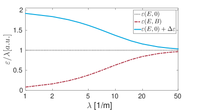
Figure 1: Qualitative comparison of the electric field energy (dotted grey line) and the effective field energy using the proposed vector potential (dot-dashed red line) for $\tau=10/m$. In addition, we show for later comparison the difference in energy ($\Delta\varepsilon$) added to the electric field energy (blue line).

This effective energy (20) for different values of $\lambda$ is displayed in Fig. 1. We find that the magnetic field can significantly reduce the effective field strength. While the electric part linearly depends on $\lambda$, the calculation for a combined electric and magnetic field shows a rapid drop off for $\tau/\lambda\gtrsim 1$.

Particle distribution

It is useful to define the reduced particle density $n(p_{x})/\lambda$ to scale out the trivial linear dependence on $\lambda$. As can be seen in Fig. 2, $n(p_{x})/\lambda$ displays a peaked structure superimposed by an oscillating function. This is characteristic for electric fields with peaks of the same absolute value but opposite sign [41].

It should be pointed out that especially the peaks in the reduced particle distribution $n(p_{x})/\lambda$ decrease with decreasing $\lambda$. A possible interpretation is that the presence of the magnetic field prevents the particles, created at the different field oscillations, to interfere. In case of $\tau/\lambda\gtrsim 1$ particles created around the first electric field oscillation at $z\neq 0$ are accelerated in $x$ and also $z$ direction. However, particles created at the second oscillation acquire a completely different momentum signature and therefore both wave packages become distinguishable. Moreover, an analysis of our data indicates, that the particle distribution is slowly shifted to lower momenta for small $\lambda$. The reason for this phenomenon seems to be directly linked with the increase in the magnetic field strength. For a configuration of the form (18), a decrease of the parameter $\lambda$ causes the region with maximal effective field amplitude to be shifted away from $t=0$. Therefore this shift has a different origin compared to the previously discovered particle self-bunching [34].

The reduced particle density $n(p_{z})/\lambda$, cf. Fig. 3, does not show any interference pattern. For $\lambda=100/m$ the distribution in $p_{z}$ is symmetric around the origin, in agreement with homogeneous calculations. However, in case of $\tau/\lambda\gtrsim 1$ the particle peak is shifted towards positive $p_{z}$.

As noted above, using the second $2$-spinor basis, one obtains a particle density mirrored at $p_{z}=0$. Therefore, this result is an indicator for interactions between the magnetic field and the electron spin.

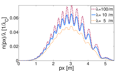
Figure 2: Reduced particle density $n(p_{x})/\lambda$ for various values of the spatial inhomogeneity $\lambda$, a field strength of $e\varepsilon=0.707\,m^{2}$ and a pulse length $\tau=5/m$. For $\lambda\gg\tau$ the reduced particle density converges.

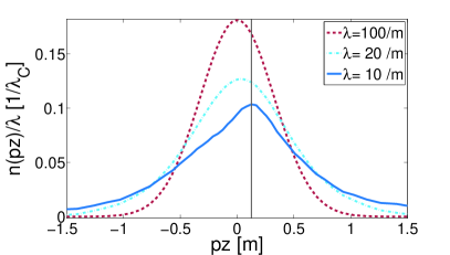
Figure 3: Reduced particle density $n(p_{z})/\lambda$ for various values of the spatial inhomogeneity $\lambda$. The particle density is symmetric for $\lambda\gg\tau$ only. The vertical grey line is there to guide the eye: the peak of the particle density is shifted to positive $p_{z}$. Parameters: $e\varepsilon=0.707\,m^{2}$ and $\tau=5/m$.

Particle yield

The magnetic field is not independent of the electric field, because both stem from the same vector potential (18). The effect of fixing $\mathbf{B}=0$ and therefore violating the homogeneous Maxwell equation $\boldsymbol{\nabla}\times\boldsymbol{E}=-\dot{\boldsymbol{B}}$ shows up in the particle density and subsequently in the particle yield. In order to draw a general conclusion between effective field energy and particles created, we will focus on the particle yield in the following.

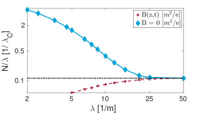
Figure 4: Double-log plot of the reduced particle yield as a function of the parameter $\lambda$. For $\lambda\gg\tau$ the reduced particle yield converges to the homogeneous result (dashed black line). In case of a sizable magnetic field the calculation for $B=0$ (blue line) leads to an overestimation compared to the correct result (dashed red line). Parameters: $\tau=10/m$ and $e\varepsilon=0.707\,m^{2}$.

The effective field energy without a magnetic field $\mathcal{E}\left(E,0\right)$ is a linear function of $\lambda$, see Fig. 1. Hence, it is reasonable to introduce an approximation for the particle yield

$$\tilde{N}=\lambda\,N_{hom},$$ (21)

where $N_{hom}$ is the yield obtained from a calculation with a spatially homogeneous field. The figures Fig. 4 and Fig. 5 show, that there is good agreement between the approximation and the full solution for $\lambda\gg\tau$. Reasons are, that in this case the electric field can be considered as quasi-homogeneous. Furthermore, the magnetic field energy is by orders of magnitude smaller than its electric counterpart and therefore negligible.

The effect of spatial restrictions on the electric field has already been investigated in Ref. [23, 34]. In our case, also the effect of a magnetic field growing in strength for decreasing $\lambda$, has to be taken into account. The corresponding computation of the effective field amplitude is depicted in Fig. 1 as $\mathcal{E}\left(E,B\right)$. One observes a faster than linear decrease. This is in qualitative agreement with the particle yield, as illustrated in Fig. 4. We have to admit, however, that for calculations with $\lambda<5/m$ the results are not reliable anymore due to a breakdown of the used Taylor expansion. (NB: The calculation with $B=0$ does not display this numerical problem.)

Eventually, the configuration $\boldsymbol{E}=-\dot{\boldsymbol{A}}$ and $\boldsymbol{B}=0$ is analyzed. Contrary to the previous case, simply calculating the effective field energy of the applied field, which would be $\mathcal{E}\left(E,0\right)$ in Fig. 1, is not sufficient. We have to consider, that the homogeneous Maxwell equations are not fulfilled. Hence, we suggest to add the missing part of the effective field energy to the electric field energy, illustrated as $\mathcal{E}\left(E,0\right)+\Delta\mathcal{E}$ in Fig. 1.

In this way, the increase in the particle yield in Fig. 4 and Fig. 5 can be understood in terms of the magnetic field. We assume, that a magnetic field hinders matter creation. Fixing $B$ to zero and ignoring the term $\boldsymbol{\nabla}\times\boldsymbol{A}$ in the equations (6)-(9) therefore inevitably leads to an overestimation of the effective field amplitude and consequently to an overestimation of the total particle number. (NB: Comparison of Fig. 1 with Fig. 4 corroborates this argument.)

The sharp drop off on the left side of Fig. 5 is connected to the fact, that for $\lambda\to 0$ the energy stored in the background field is not sufficient anymore to overcome the particle rest mass [17, 23].

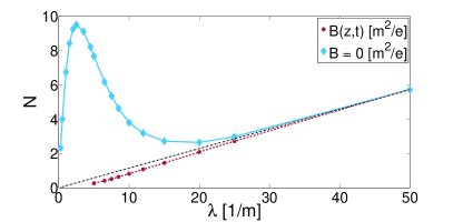
Figure 5: Particle yield drawn in a lin-lin plot for a configuration with $\tau=10/m$ and $e\varepsilon=0.707\,m^{2}$ (the same set of data as in Fig. 4 is used). At $\lambda=5/m$ the particle yield obtained from a calculation with $B=0$ exceeds the correct result by a factor of $50$.

Conclusions

Based on the DHW formalism, Sauter-Schwinger electron-positron pair production in time-dependent, spatially inhomogeneous electric and magnetic fields has been investigated. For the first time the equations of motion for an effectively $2+1$ dimensional system has been solved numerically. We have focused on the influence of the magnetic field on the pair production process for a special class of vector potentials. We have found that for this kind of potentials the magnetic field is of minor importance for a wide range of parameter sets thereby validating studies which have been performed so far. Additionally, there is perfect agreement in the results when comparing to quantum kinetic theory in the limit of spatially homogeneous fields. However, and as most important result presented here, we have verified in a quantitative manner that in the case of spatially strongly localized fields the results can be explained assuming that pair production is only possible in regions where the electric field exceeds the magnetic field. In this parameter region the correct treatment of the magnetic field is of utter importance.

Outlook

In order to investigate pair production in background fields with more realistic length and time scales, improvements in the employed numerical methods will be necessary. Such work is in progress, and it will allow to investigate more general electromagnetic fields. A possible extension would be, for example, the study of multi-photon pair production. Therefore we are optimistic that the investigation presented here will soon serve as a basis for studies employing fields closer to experimentally feasible conditions.

References

- [1] F. Sauter, Z. Phys. 69, 742 (1931); W. Heisenberg and H. Euler, Z. Phys. 98, 714 (1936); J. S. Schwinger, Phys. Rev. 82, 664 (1951);
- [2] D. L. Burke, R. C. Field, G. Horton-Smith, T. Kotseroglou, J. E. Spencer, D. Walz, S. C. Berridge and W. M. Bugg et al., Phys. Rev. Lett. 79 (1997) 1626; C. Bamber, S. J. Boege, T. Koffas, T. Kotseroglou, A. C. Melissinos, D. D. Meyerhofer et al., Phys. Rev. D 60, 092004 (1999);
- [3] Proposal for a European Extreme Light Infrastructure (ELI), http://www.eli-laser.eu/;
- [4] T. Heinzl and A. Ilderton, Eur. Phys. J. D 55 (2009) 359 [arXiv:0811.1960 [hep-ph]];
- [5] XFEL, http://www.xfel.eu/de/, The HIBEF project, http://www.hzdr.de/db/Cms?pNid=427&pOid=35325;
- [6] A. Ringwald, Phys. Lett. B 510 (2001) 107 [hep-ph/0103185];
- [7] M. Marklund and J. Lundin, Eur. Phys. J. D 55 (2009) 319 [arXiv:0812.3087 [hep-th]]; O. J. Pike, F. Mackenroth, E. G. Hill and S. J. Rose, Nature Photon. (2014);
- [8] G. V. Dunne, In *Shifman, M. (ed.) et al.: From fields to strings, vol. 1* 445-522 [hep-th/0406216];
- [9] R. Alkofer, M. B. Hecht, C. D. Roberts, S. M. Schmidt and D. V. Vinnik, Phys. Rev. Lett. 87, 193902 (2001);
- [10] R. Schützhold, H. Gies and G. Dunne, Phys. Rev. Lett. 101 (2008) 130404.
- [11] C. Kohlfürst, H. Gies and R. Alkofer, Phys. Rev. Lett. 112 (2014) 050402 [arXiv:1310.7836 [hep-ph]]; A. Blinne and H. Gies, Phys. Rev. D 89 (2014), 085001 [arXiv:1311.1678 [hep-ph]]; A. Huet, S. P. Kim and C. Schubert, Phys. Rev. D 90 (2014) 125033 [arXiv:1411.3074 [hep-th]]; I. Akal, S. Villalba-Chávez and C. Müller, Phys. Rev. D 90 (2014) 113004 [arXiv:1409.1806 [hep-ph]]; A. Otto, D. Seipt, D. Blaschke, B. Kampfer and S. A. Smolyansky, Phys. Lett. B 740 (2015) 335 [arXiv:1412.0890 [hep-ph]];
- [12] D. Cangemi, E. D’Hoker and G. V. Dunne, Phys. Rev. D 52 (1995) 3163 [hep-th/9506085]; G. V. Dunne and T. M. Hall, Phys. Lett. B 419 (1998) 322 [hep-th/9710062]; S. P. Kim and D. N. Page, Phys. Rev. D 75 (2007) 045013 [hep-th/0701047]; R. Ruffini, G. Vereshchagin and S. S. Xue, Phys. Rept. 487 (2010) 1 [arXiv:0910.0974 [astro-ph.HE]]; M. Jiang, Q. Z. Lv, Y. Liu, R. Grobe and Q. Su, Phys. Rev. A 90 (2014) 032101; A. Ilderton, G. Torgrimsson and J. Wårdh, Phys. Rev. D 92 (2015) 065001, [arXiv:1506.09186 [hep-th]];
- [13] F. Mackenroth and A. Di Piazza, Phys. Rev. A 83 (2011) 032106 [arXiv:1010.6251 [hep-ph]]; T. Nousch, D. Seipt, B. Kampfer and A. I. Titov, Phys. Lett. B 715 (2012) 246;
- [14] C. Kohlfürst, PhD Thesis (2015) [arXiv:1512.06082 [hep-ph]];
- [15] C. Kohlfürst, H. Gies and R. Alkofer, Phys. Rev. Lett. 112 (2014) 050402, [arXiv:1310.7836 [hep-ph]];
- [16] M. Ruf, G. R. Mocken, C. Muller, K. Z. Hatsagortsyan and C. H. Keitel, Phys. Rev. Lett. 102 (2009) 080402 [arXiv:0810.4047 [physics.atom-ph]];
- [17] F. Hebenstreit, arXiv:1106.5965 [hep-ph];
- [18] T. D. Cohen and D. A. McGady, Phys. Rev. D 78 (2008) 036008 [arXiv:0807.1117 [hep-ph]]; F. Gelis and N. Tanji, arXiv: 1510.05451 [hep-ph];
- [19] M. Orthaber, F. Hebenstreit and R. Alkofer, Phys. Lett. B 698 (2011) 80 doi:10.1016/j.physletb.2011.02.053 [arXiv:1102.2182 [hep-ph]].
- [20] M. F. Linder, C. Schneider, J. Sicking, N. Szpak and R. Schützhold, Phys. Rev. D 92 (2015) 085009 doi:10.1103/PhysRevD.92.085009 [arXiv:1505.05685 [hep-th]].
- [21] A. D. Panferov, S. A. Smolyansky, A. Otto, B. Kaempfer, D. Blaschke and L. Juchnowski, arXiv:1509.02901 [quant-ph].
- [22] A. Di Piazza and G. Calucci, Astroparticle Physics 24 (2006) 520;
- [23] G. V. Dunne and C. Schubert, Phys. Rev. D 72 (2005) 105004 [hep-th/0507174]; H. Gies and K. Klingmuller, Phys. Rev. D 72 (2005) 065001 [hep-ph/0505099];
- [24] C. Schneider and R. Schützhold, arXiv:1407.3584 [hep-th];
- [25] C. K. Dumlu and G. V. Dunne, Phys. Rev. Lett. 104 (2010) 250402 [arXiv:1004.2509 [hep-th]]; H. Kleinert and S. S. Xue, Annals Phys. 333 (2013) 104 [arXiv:1207.0401 [physics.plasm-ph]]; E. Strobel and S. S. Xue, Nucl. Phys. B 886 (2014) 1153 [arXiv:1312.3261 [hep-th]];
- [26] S. A. Smolyansky, G. Ropke, S. M. Schmidt, D. Blaschke, V. D. Toneev and A. V. Prozorkevich, hep-ph/9712377; Y. Kluger, E. Mottola and J. M. Eisenberg, Phys. Rev. D 58, 125015 (1998); S. M. Schmidt, D. Blaschke, G. Ropke, S. A. Smolyansky, A. V. Prozorkevich and V. D. Toneev, Int. J. Mod. Phys. E 7, 709 (1998); J. C. R. Bloch, V. A. Mizerny, A. V. Prozorkevich, C. D. Roberts, S. M. Schmidt, S. A. Smolyansky and D. V. Vinnik, Phys. Rev. D 60 (1999) 116011 [nucl-th/9907027];
- [27] R. Dabrowski and G. V. Dunne, Phys. Rev. D 90 (2014) 025021 [arXiv:1405.0302 [hep-th]];
- [28] C. Kohlfurst, M. Mitter, G. von Winckel, F. Hebenstreit and R. Alkofer, Phys. Rev. D 88 (2013) 045028 [arXiv:1212.1385 [hep-ph]];
- [29] F. Hebenstreit and F. Fillion-Gourdeau, Phys. Lett. B 739 (2014) 189 [arXiv:1409.7943 [hep-ph]];
- [30] F. Hebenstreit, arXiv:1509.08693 [hep-ph];
- [31] A. Blinne and E. Strobel, arXiv:1510.02712 [hep-ph];
- [32] Z. L. Li, D. Lu, B. F. Shen, L. B. Fu, J. Liu and B. S. Xie, arXiv:1410.6284 [hep-ph];
- [33] D. Berényi, S. Varró, V. V. Skokov and P. Lévai, Phys. Lett. B 749 (2015) 210 [arXiv:1401.0039 [hep-ph]];
- [34] F. Hebenstreit, R. Alkofer and H. Gies, Phys. Rev. Lett. 107 (2011) 180403 [arXiv:1106.6175 [hep-ph]];
- [35] H. Kleinert, R. Ruffini and S. S. Xue, Phys. Rev. D 78 (2008) 025011 [arXiv:0807.0909 [hep-th]]; W. B. Han, R. Ruffini and S. S. Xue, Phys. Lett. B 691 (2010) 99 [arXiv:1004.0309 [hep-ph]]; F. Hebenstreit, J. Berges and D. Gelfand, Phys. Rev. D 87 (2013) 105006 [arXiv:1302.5537 [hep-ph]];
- [36] C. Harvey, T. Heinzl, A. Ilderton and M. Marklund, Phys. Rev. Lett. 109 (2012) 100402 [arXiv:1203.6077 [hep-ph]];
- [37] D. Vasak, M. Gyulassy and H. T. Elze, Annals Phys. 173 (1987) 462; I. Bialynicki-Birula, P. Górnicki and J. Rafelski, Phys. Rev. D 44 (1991); P. Zhuang, U. Heinz, Ann.Phys.245:311-338,1996 [arXiv:nucl-th/9502034];
- [38] M. de Jesus Anguiano Galicia and A. Bashir, Few Body Syst. 37 (2005) 71 [hep-ph/0502089];
- [39] J. P. Boyd, Dover Books on Mathematics (2001), ISBN : 9780486411835;
- [40] W. H. Press, S. A. Teukolsky, W. T. Vetterling and B. P. Flannery Cambridge University Press ISBN-13: 978-0521880688;
- [41] F. Hebenstreit, R. Alkofer, G. V. Dunne and H. Gies, Phys. Rev. Lett. 102 (2009) 150404 [arXiv:0901.2631 [hep-ph]]; E. Akkermans and G. V. Dunne, Phys. Rev. Lett. 108 (2012) 030401 [arXiv:1109.3489 [hep-th]]; T. Heinzl, A. Ilderton and M. Marklund, Phys. Lett. B 692 (2010) 250, [arXiv:1002.4018 [hep-ph]];