Abstract

We study the boundary conditions in topologically twisted Chern-Simons matter theories with the Lie 3-algebraic structure. We find that the supersymmetric boundary conditions and the gauge invariant boundary conditions can be unified as complexified gauge invariant boundary conditions which lead to supergroup WZW models. We propose that the low-energy effective field theories on the two-dimensional intersection of multiple M2-branes on a holomorphic curve inside K3 with two non-parallel M5-branes on the K3 are supergroup WZW models from the topologically twisted BLG-model and the ABJM-model.

1 Introduction

One of the most important clues to understanding M-theory is the investigation of the two types of branes, namely M2-branes and M5-branes. It has been proposed that the low-energy dynamics of multiple M2-branes probing a flat space is described by three-dimensional superconformal Chern-Simons matter theories known as the BLG-model [1, 2, 3, 4, 5] and the ABJM-model [6]. The world-volume theory of the M5-branes is believed to be a six-dimensional $\mathcal{N}=(2,0)$ superconformal field theory. It is much less understood due to the lack of a classical Lagrangian description, although there have been many interesting discoveries via its compactification. Also the two-dimensional intersection of M2-branes with M5-branes still remains elusive. This brane setup is believed to be one of the most promising approaches to the description of the M5-branes as it is realized when the strongly coupled $(2,0)$ theory is away from the conformal fixed point.

The aim of the present paper is to study the two-dimensional intersection of multiple M2-branes on a supersymmetric two-cycle. In particular, we consider a holomorphic curve inside K3 with two non-parallel M5-branes on the K3, which we will refer to as M5- and M5’-branes. We investigate the low-energy effective description by starting with the topologically twisted Chern-Simons matter theories describing the M2-branes on the holomorphic curve and examining the boundary conditions. Given the brane configuration of the M2-M5-M5’ branes on the K3, we determine the boundary conditions for the matter fields as supersymmetric boundary conditions while we impose those on the gauge fields as gauge invariant boundary conditions. We find that these two different types of boundary conditions can be combined into complexified gauge invariant boundary conditions. Together with the twisted fermionic fields, i.e. the spin zero fermions and the spin one fermions, we obtain conformal field theories on the Riemann surface as the $PSL(2|2)$ WZW action from the twisted BLG-model and the $GL(N|N)$ WZW action from the twisted $U(N)_{k}\times U(N)_{-k}$ ABJM-model. We propose that such supergroup WZW models are realized as the effective topological theories on the intersection of the M2-M5-M5’ system on K3, which we will call “topological M-strings”.

The paper is organized as follows. In section 2 we present a brane configuration in M-theory on K3 and establish our setup of the topological M-strings. We describe the world-volume theory on the M2-branes wrapping a holomorphic curve inside K3 by performing a partial topological twist on the BLG-model [7]. In section 3 we analyze the boundary conditions of the topologically twisted BLG theory. The matter fields satisfy the supersymmetric boundary conditions imposed by the fivebrane while the gauge fields obey the gauge invariant boundary conditions so that we keep the combined system of the M2-branes [8]. We find the merging of the two boundary conditions as complexified gauge invariant boundary conditions. In section 4 we derive the boundary action by taking into account the boundary conditions. We argue that the complexified gauge invariant boundary conditions lead to the sum of the WZW models for complexified gauge group. By putting together the conformally invariant terms involving the twisted fermions, which are known as symplectic fermions [9], i.e. fermionic scalar fields and fermionic one-form fields, we find the supergroup WZW models. We propose that the supergroup WZW models are the conformally invariant effective theories of the topological M-strings. Finally in section 5 we close with some discussion.

2 Topological M-strings

We consider M-theory on the background

$$\mathrm{K3}\times\mathbb{R}^{7}.$$ (2.1)

We take the K3 as a cotangent bundle $T^{*}\Sigma_{g}$ over a Riemann surface $\Sigma_{g}$ where $\Sigma_{g}$ is a holomorphic curve of genus $g\neq 1$ in the $x^{0}$, $x^{1}$ directions . We take the non-trivial normal bundle $N_{\Sigma}$ over the surface in the $x^{9}$, $x^{10}$ directions. Let us consider multiple wrapped M2-branes on $\Sigma_{g}\times I$ where $I$ is an interval in the $x^{2}$ direction with length $L$. At one end of the interval we put a single fivebrane on $\mathrm{K3}\times\mathbb{R}^{2}_{34}$, which we will call an M5-brane, and at the other end a fivebrane on $\mathrm{K3}\times\mathbb{R}^{2}_{56}$, which we will call an M5’-brane. The configuration is summarized as

$$\begin{array}[]{cccccccccccc}&0&1&2&3&4&5&6&7&8&9&10\\ \textrm{M5}&\circ&\circ&&\circ&\circ&&&&&\circ&\circ\\ \textrm{M5'}&\circ&\circ&&&&\circ&\circ&&&\circ&\circ\\ \textrm{M2}&\circ&\circ&\circ&&&&&&&&\\ \end{array}$$ (2.6)

and it is depicted in Figure 1.

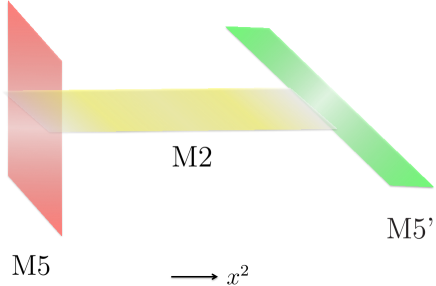
Figure 1: M2-branes stretched between an M5-brane and an M5’-brane along the $x^{2}$ direction.

Since the K3 decomposes the holonomy group $SO(4)$ of the flat four-manifold into $SU(2)$, the spinor representation follows the branching rule $\bm{4}$ $\rightarrow$ $\bm{2}\oplus\bm{1}\oplus\bm{1}$ and there remains half of the supersymmetry, sixteen supercharges in the M-theory background (2.1). The presence of the M2-branes, the M5-brane and the M5’-brane splits the $SO(7)$ Euclidean symmetry group into $SO(2)_{34}\times SO(2)_{56}\times SO(2)_{78}$ and breaks $1/8$ of the background supersymmetry as a consequence of three projections. Altogether, there are two supercharges preserved on the world-volume of the branes.

As the fivebranes are infinite in the directions which are not shared by the membranes, the fivebranes are much heavier than the membranes. Thus the parameters of the fivebranes would be fixed and the low-energy effective theory of the branes would essentially describe the stretched M2-branes. The M2-branes represent minimum energy states in a specific topological sector as BPS states. We consider the field theory of the membranes in which the distance $L$ goes to zero and thus it is a two-dimensional sigma model on the intersection. The target space of this sigma model would be the moduli space of solutions to the BPS constraints which encompass the supersymmetric boundary conditions. In what follows we will consider such effective theories on the M2-branes. Recently there have been intriguing approaches for the study of M2-branes stretched between M5-branes, the so-called M-strings [10]. In our brane setup (2.6) the M2-branes cannot fluctuate in the flat directions, i.e. in $x^{3}$, $x^{4}$, $\cdots$, $x^{8}$, so the effective theories on the wrapped M2-branes may only capture the topological sector of the M-strings, which we call the topological M-strings. We will seek the topological sigma model on the intersection as the effective theory of the topological M-strings.

The low-energy effective theory of curved branes wrapping supersymmetric cycles can be obtained by a topological twisting of an effective theory of flat branes propagating in a flat space [11]. We shall firstly discuss the case of two M2-branes. The low-energy effective theory of two coincident membranes propagating in a flat space $\mathbb{R}^{8}$ is expected to be realized as the BLG-model [1, 2, 3, 4, 5]. The BLG-model is a three-dimensional $\mathcal{N}=8$ superconformal Chern-Simons matter theory whose action is

$$S_{\textrm{BLG}} =S_{\textrm{matter}}+S_{\textrm{TCS}}$$ (2.7)

where

$$S_{\textrm{matter}} =\int d^{3}x\Biggl{[}-\frac{1}{2}D^{\mu}X^{Ia}D_{\mu}X_{a}^{I}+\frac{i}{2}\overline{\Psi}^{a}\Gamma^{\mu}D_{\mu}\Psi_{a}$$

$$+\frac{i}{4}\overline{\Psi}_{b}\Gamma^{IJ}X^{I}_{c}X^{J}_{d}\Psi_{a}f^{abcd}-\frac{1}{12}f^{abcd}{f^{efg}}_{d}X_{a}^{I}X_{b}^{J}X_{c}^{K}X_{e}^{I}X_{f}^{J}X_{g}^{K}\Biggr{]}$$ (2.8)

is the matter action and

$$S_{\textrm{TCS}} =\frac{1}{2}\epsilon^{\mu\nu\lambda}\left(f^{abcd}A_{\mu ab}\partial_{\nu}A_{\lambda cd}+\frac{2}{3}{f^{cda}}_{g}f^{efgb}A_{\mu ab}A_{\nu cd}A_{\lambda ef}\right)$$ (2.9)

is the twisted Chern-Simons action in terms of the structure constants ${f^{abc}}_{d}$ of the Lie 3-algebra. Only the $\mathcal{A}_{4}$ algebra with ${f^{abc}}_{d}=\frac{2\pi}{k}\epsilon^{abcd}$, $k\in\mathbb{Z}$, $a,b,\cdots,=1,\cdots,4$ admits a finite dimensional non-trivial representation of the Lie 3-algebra with a positive definite metric. The field content is eight real scalar fields $X^{I}_{a}$, $I=1,\cdots,8$ describing the position of the M2-branes in the flat eight-dimensional space, fermionic fields $\Psi_{a}$ defined as the $SO(1,10)$ Majorana spinor obeying the projection $\Gamma_{012}\Psi=-\Psi$ and gauge fields $A_{\mu ab}$, $\mu=0,1,2$ where the gauge indices $a,b,\cdots$ run from $1$ to $4$. The theory has a three-dimensional Lorentz group $SO(1,2)$ as the rotational symmetry group on the world-volume of the membranes and the R-symmetry group $SO(8)_{R}$ as the isometry of the transverse space of the membranes. The fields $X^{I}_{a}$, $\Psi_{a}$ and $A_{\mu ab}$ transform under the $SO(1,2)\times SO(8)_{R}$ as $(\bm{1},\bm{8}_{v})$, $(\bm{2},\bm{8}_{c})$ and $(\bm{3},\bm{1})$ respectively. The action (2.7) is invariant under the supersymmetry transformations

$$\delta X_{a}^{I} =i\overline{\epsilon}\Gamma^{I}\Psi_{a}$$ (2.10)

$$\delta\Psi_{a} =D_{\mu}X_{a}^{I}\Gamma^{\mu}\Gamma^{I}\epsilon-\frac{1}{6}X_{b}^{I}X_{c}^{J}X_{d}^{K}{f^{bcd}}_{a}\Gamma^{IJK}\epsilon$$ (2.11)

$${{\delta\tilde{A}_{\mu}}^{b}}_{a} =i\overline{\epsilon}\Gamma_{\mu}\Gamma^{I}X_{c}^{I}\Psi_{d}{f^{cdb}}_{a}$$ (2.12)

where we have defined ${\tilde{A}_{\mu}}{\ {}^{b}}_{a}:={f^{cdb}}_{a}A_{\mu cd}$. The supersymmetry parameter $\epsilon$ is the $SO(1,10)$ Majorana spinor satisfying the projection $\Gamma_{012}\epsilon=\epsilon$ and transforms as $(\bm{2},\bm{8}_{s})$.

In order to study the two wrapped M2-branes on a holomorphic Riemann surface $\Sigma_{g}$, we consider a partial topological twisting of the BLG-model. Such a topological twisting replaces the Euclidean symmetry group $SO(2)_{E}$ of the two-dimensional space by a different subgroup $SO(2)_{E}^{\prime}$ of the $SO(2)_{E}\times SO(8)_{R}$ so that there exist scalar supercharges as discussed in [7]. There are plenty of twists by taking a homomorphism $\mathfrak{h}$: $SO(2)\rightarrow SO(8)_{R}$. The partial topological twisting for the M2-branes wrapped on a holomorphic curve inside K3 can be uniquely determined by decomposing the $SO(8)_{R}$ $\rightarrow$ $SO(2)_{R}\times SO(6)_{R}$ and defining $SO(2)^{\prime}_{E}$ $=$ $\mathrm{diag}(SO(2)_{E}\times SO(2)_{R})$. After the twist the bosonic matter fields transform under $SO(2)_{E}^{\prime}\times SO(6)_{R}$ as

$$\bm{6}_{0}\oplus\bm{1}_{2}\oplus\bm{1}_{-2}$$ (2.13)

and one obtains the resultant bosonic scalar fields $\bm{6}_{0}$ which we denote by $\phi^{I}$, where now $I=1,\cdots,6$ and a bosonic one-form $\bm{1}_{2}$ and $\bm{1}_{-2}$ which we denote by $\Phi_{z}$ and $\Phi_{\overline{z}}$. The representation of the fermionic fields is

$$\bm{4}_{2}\oplus\overline{\bm{4}}_{0}\oplus\bm{4}_{0}\oplus\overline{\bm{4}}_{-2}$$ (2.14)

where $\bm{4}_{0}$, $\overline{\bm{4}}_{0}$ are the fermionic scalar fields which we will denote by $\psi$, $\tilde{\lambda}$ while $\bm{4}_{2}$, $\overline{\bm{4}}_{-2}$ are the fermionic one-form fields which we will denote by $\Psi_{z}$, $\tilde{\Psi}_{\overline{z}}$. The supersymmetry parameter $\epsilon$ transforms as

$$\bm{4}_{0}\oplus\overline{\bm{4}}_{2}\oplus\bm{4}_{-2}\oplus\overline{\bm{4}}_{0}$$ (2.15)

under $SO(2)_{E}^{\prime}\times SO(6)$ and thus one can find eight scalar supercharges associated with the supersymmetric parameters $\xi$, $\tilde{\xi}$ in the representation $\bm{4}_{0}\oplus\overline{\bm{4}}_{0}$. Note that topological twisting modifies the original theory so that the new symmetry group $SO(2)_{E}^{\prime}$ is defined by the diagonal subgroup of $SO(2)_{E}$ and $SO(2)_{R}=SO(2)_{910}$ as diag$(SO(2)_{E}\times SO(2)_{910})$. In other words, the new generator of $SO(2)^{\prime}_{E}$ has been created by the generator of $SO(2)_{E}$ and that of $SO(2)_{910}$. So we could only say that the resulting twisted theory contains the modified $SO(2)_{E}^{\prime}$ symmetry group.

From the M-theory point of view, a compactification on K3 retains seven flat directions and six of them are transverse to the membranes’ world-volume $\Sigma_{g}\times I$. Thus we see that the above topological twisting exactly realizes the required bosonic field content in the effective theory of the M2-branes wrapped on $\Sigma_{g}$ inside K3. The six bosonic scalars $\phi^{I}$ describe the displacement of the M2-branes in the six flat directions while the bosonic one-form field $\Phi_{\alpha}$ on the Riemann surface describes the motion of the M2-branes inside K3, i.e. the non-trivial normal bundle $N_{\Sigma}$ over $\Sigma_{g}$. The existence of eight covariantly constant spinors in (2.15) reflects the fact that K3 breaks half of the supersymmetry.

3 Boundary Conditions

3.1 Supersymmetric boundary conditions

To extend the study of the compact M2-branes wrapped around a holomorphic curve inside K3 to the M2-M5-M5’ system (2.6), we will analyze the boundary conditions which should be imposed by the M5-brane and the M5’-brane at the ends of the M2-branes in the $x^{2}$ direction. Let us start our investigation by considering maximally supersymmetric boundary conditions, i.e. half-BPS boundary conditions of the BLG-model which include the case where the M2-branes end on an M5-brane .

The supersymmetry is preserved on the boundary when the normal component of the supercurrent vanishes on the boundary [13, 12, 14, 15]. The supersymmetric transformations (2.10)-(2.12) lead to a supercurrent

$$J^{\mu} =-D_{\nu}X^{Ia}\Gamma^{\nu}\Gamma^{I}\Gamma^{\mu}\Psi_{a}-\frac{1}{6}X_{a}^{I}X_{b}^{J}X_{c}^{K}f^{abcd}\Gamma^{IJK}\Gamma^{\mu}\Psi_{d}.$$ (3.1)

Let the M2-branes with world-volume $(x^{0},x^{1},x^{2})$ end on a single M5-brane with world-volume $(x^{0},x^{1},x^{3},x^{4},x^{9},x^{10})$ at, say, $x^{2}=0$. According to the existence of the M5-brane the $SO(8)_{R}$ splits into $SO(4)_{34910}\times SO(4)_{5678}$. Correspondingly we will decompose the eight scalar fields into two parts; $X^{i}$ $=$ $\left\{X^{3},X^{4},X^{9},X^{10}\right\}$, $Y^{\hat{i}}$ $=$ $\left\{X^{5},X^{6},X^{7},X^{8}\right\}$. Then the supersymmetric boundary conditions can be written as

$$0 =\overline{\epsilon}J^{2}\Big{|}_{\textrm{bdy}}$$

$$=D_{\alpha}X^{i}\left(\overline{\epsilon}\Gamma^{i\alpha 2}\Psi\right)+D_{\alpha}Y^{\hat{i}}\left(\overline{\epsilon}\Gamma^{\hat{i}\alpha 2}\Psi\right)$$

$$+D_{2}X^{i}\left(\overline{\epsilon}\Gamma^{i}\Psi\right)+D_{2}Y^{\hat{i}}\left(\overline{\epsilon}\Gamma^{\hat{i}}\Psi\right)$$

$$-\frac{1}{6}\left[X^{i},X^{j},X^{k}\right]\left(\overline{\epsilon}\Gamma^{ijk}\Gamma^{2}\Psi\right)-\frac{1}{6}\left[Y^{\hat{i}},Y^{\hat{j}},Y^{\hat{k}}\right]\left(\overline{\epsilon}\Gamma^{\hat{i}\hat{j}\hat{k}}\Gamma^{2}\Psi\right)$$

$$-\frac{1}{2}\left[X^{i},X^{j},Y^{\hat{k}}\right]\left(\overline{\epsilon}\Gamma^{ij\hat{k}}\Gamma^{2}\Psi\right)-\frac{1}{2}\left[X^{i},Y^{\hat{j}},Y^{\hat{k}}\right]\left(\overline{\epsilon}\Gamma^{i\hat{j}\hat{k}}\Gamma^{2}\Psi\right)\Bigg{|}_{\textrm{bdy}}.$$ (3.2)

To find the solutions to the half-BPS boundary conditions which correspond to the M2-M5 system, we should take into account several constraints from the brane configuration. We observe that all the parameters of the M5-brane are fixed so that the scalar fields $Y^{\hat{i}}$ should obey the Dirichlet boundary conditions $D_{\alpha}Y^{\hat{i}}=0$. Since we do not expect the M5-brane to impose both Neumann and Dirichlet boundary conditions on the scalar fields $Y^{\hat{i}}$, $D_{2}Y^{\hat{i}}=0$ should not also be constrained at the boundary. Therefore, in order to satisfy the boundary condition (3.1) we also need to choose appropriate boundary conditions for the fermionic fields.

Noting that the unbroken supersymmetry parameter $\epsilon$ must satisfy the projections $\Gamma_{0134910}\epsilon=\epsilon$ due to the M5-brane and $\Gamma_{012}\epsilon=\epsilon$ due to the M2-branes, one finds

$$\Gamma_{01}\epsilon=\Gamma_{2}\epsilon=\Gamma_{34910}\epsilon=\Gamma_{5678}\epsilon.$$ (3.3)

There remain eight supercharges on the two-dimensional boundary. In two dimensions supersymmetry has a definite chirality. Equation (3.3) shows that the chiralities of the supersymmetry parameter under the $SO(1,1)_{01}$, the $SO(4)_{34910}$ and the $SO(4)_{5678}$ are the same. It is easily checked that $\Gamma_{01}$ is Hermitian, traceless and squares to the identity on the eight-dimensional subspace of spinors satisfying equation (3.3). Thus $\mathcal{N}=(4,4)$ supersymmetry is preserved on the two-dimensional boundary of the M2-branes ending on the M5-brane.

As in the projection conditions (3.3), we can employ the boundary condition ansatz for the fermions $\Gamma_{0134910}\Psi=\Psi$ so that the space-time symmetry of the brane configuration is maintained. Combining the boundary conditions (3.1) with the fermionic boundary conditions satisfying the restrictions from the M2-M5 configuration we get the half-BPS boundary conditions at the M5-brane

$$D_{2}X^{i}+\frac{1}{6}\epsilon^{ijkl}[X^{j},X^{k},X^{l}]\Bigl{|}_{\textrm{bdy}} =0,$$ (3.4)

$$D_{\alpha}Y^{\hat{i}}\Bigl{|}_{\textrm{bdy}} =0$$ (3.5)

where $\epsilon^{ijkl}$ is an antisymmetric tensor with $\epsilon^{34910}=1$ . The first boundary condition (3.4) is the Basu-Harvey equation [16] which would describe the displacement of the M2-branes in the four-dimensional space inside the M5-brane. The second boundary condition (3.5) fixes the boundary values of the position of the M2-branes in the remaining four-dimensional space which is normal to the M5-brane.

One can easily obtain the boundary conditions from an additional fivebrane. Consider the fivebrane with world-volume $(x^{0},x^{1},x^{5},x^{6},x^{7},x^{8})$, which we will denote by $\widetilde{\textrm{M5}}$-brane. By exchanging a role of $X^{i}$ and $Y^{\hat{i}}$, we obtain the boundary conditions

$$D_{2}Y^{\hat{i}}+\frac{1}{6}\epsilon^{\hat{i}\hat{j}\hat{k}\hat{l}}[Y^{\hat{j}},Y^{\hat{k}},Y^{\hat{l}}]\Bigl{|}_{\textrm{bdy}} =0,$$ (3.6)

$$D_{\alpha}X^{i}\Bigl{|}_{\textrm{bdy}} =0.$$ (3.7)

Adding the boundary conditions (3.6) and (3.7) from the $\widetilde{\textrm{M5}}$-brane to the boundary conditions (3.4) and (3.5) from the M5-brane does not break further supersymmetry. So the effective theories of the intersecting M2-M5-$\widetilde{\textrm{M5}}$ system in a flat space would be two-dimensional $\mathcal{N}=(4,4)$ superconformal field theories. Although the knowledge of such field theories is still limited, the M2-M5-$\widetilde{\textrm{M5}}$ solutions whose near-horizon geometries take the form AdS${}_{3}\times$ $S^{3}\times$ $S^{3}$ have been constructed in the gravity dual perspective [17, 18, 19].

Let us instead consider the flat M5’-brane located along $(x^{0},x^{1},x^{5},x^{6},x^{9},x^{10})$ having four common directions with the M5-brane. The isometry of the transverse space of the M2-branes reduces to $SO(2)_{34}\times SO(2)_{56}\times SO(2)_{78}\times SO(2)_{910}$. We thus decompose the eight scalar fields as $X^{i}=(X^{9},X^{10})$, $Y^{\hat{i}}=(X^{7},X^{8})$, $Z^{i}=(X^{3},X^{4})$ and $\hat{Z}^{\hat{i}}=(X^{5},X^{6})$. The preserved supersymmetry parameters $\epsilon$ should satisfy $\Gamma_{012}\epsilon=\epsilon$, $\Gamma_{0134910}\epsilon=\epsilon$ and $\Gamma_{0156910}\epsilon=\epsilon$, from which one can read their chiralities under the $SO(1,1)_{01}\times SO(2)_{34}\times SO(2)_{56}\times SO(2)_{78}\times SO(2)_{910}$ as $(+,+,+,-,-)$, $(+,-,-,+,+)$, $(-,+,+,+,+)$ and $(-,-,-,-,-)$. Thus $\mathcal{N}=(2,2)$ supersymmetry is preserved on the two-dimensional intersection of the M2-M5-M5’ system.

Adopting the fermionic boundary conditions $\Gamma_{0134910}\Psi=\Psi$ on the M5-brane and $\Gamma_{0156910}\Psi=\Psi$ on the M5’-brane, in the limit where the M5-M5’ separation is small, we find the common set of boundary conditions on the bosonic fields

$$D_{2}X^{i}+\frac{1}{2}\epsilon^{ijkl}[X^{j},Z^{k},Z^{l}]+\frac{1}{2}\epsilon^{ij\hat{k}\hat{l}}[X^{j},\hat{Z}^{\hat{k}},\hat{Z}^{l}]=0,$$ (3.8)

$$D_{\alpha}Y^{\hat{i}}=0,$$ (3.9)

$$D_{\alpha}Z^{i}=0,\ \ \ \ \ D_{2}Z^{i}+\frac{1}{2}\epsilon^{ijkl}[Z^{j},X^{k},X^{l}]=0,$$ (3.10)

$$D_{\alpha}\hat{Z}^{\hat{i}}=0,\ \ \ \ \ D_{2}\hat{Z}^{\hat{i}}+\frac{1}{2}\epsilon^{\hat{i}\hat{j}kl}[\hat{Z}^{\hat{j}},X^{k},X^{l}]=0.$$ (3.11)

The first equation (3.8) is the Basu-Harvey like equation for $X^{i}$ with two of the elements in the three bracket replaced by $Z^{i}$ or $\hat{Z}^{\hat{i}}$. The second equation (3.9) is the Dirichlet boundary condition on $Y^{\hat{i}}$. The last two equations are curious since the $Z^{i}$ and $\hat{Z}^{\hat{i}}$ are required to be fixed at the boundary by one of the fivebranes while they should also keep the Lie 3-algebraic structure due to the non-vanishing three-bracket. Although the direct analysis of the $\mathcal{N}=(2,2)$ superconformal field theories is still difficult, their supersymmetric ground states, the chiral rings, the BPS spectra and the sphere partition functions have been investigated by taking the mass deformation in [20].

Now we will proceed to the boundary conditions in the topologically twisted BLG theory describing the curved M2-branes. Let us decompose the $SO(1,10)$ gamma matrices as

$$\begin{cases}\Gamma^{\mu}=\gamma^{\mu}\otimes\hat{\Gamma}^{7}\otimes\sigma_{2}&\mu=0,1,2\cr\Gamma^{I+2}=\mathbb{I}_{2}\otimes\hat{\Gamma}^{I}\otimes\sigma_{2}&I=1,\cdots,6\cr\Gamma^{i+8}=\mathbb{I}_{2}\otimes\mathbb{I}_{8}\otimes\gamma^{i}&i=1,2\cr\end{cases}$$ (3.12)

where $\gamma^{\mu}$, $\mu=0,1,2$ are $2\times 2$ matrices; $\gamma^{0}=\sigma_{1}$, $\gamma^{1}=\sigma_{3}$ and $\gamma^{2}=i\sigma_{2}$, while $\hat{\Gamma}^{I}$ are the $SO(6)$ gamma matrices satisfying the relations

$$\{\hat{\Gamma}^{I},\hat{\Gamma}^{J}\}=2\delta^{IJ},\ \ \ (\hat{\Gamma}^{I})^{{\dagger}}=\Gamma^{I},$$ (3.13)

$$\hat{\Gamma}^{7}=-i\hat{\Gamma}^{12\cdots 6}=\left(\begin{array}[]{cc}\mathbb{I}_{4}&0\\ 0&-\mathbb{I}_{4}\\ \end{array}\right).$$ (3.16)

The $SO(1,10)$ charge conjugation matrix $\mathcal{C}$ is decomposed as

$$\mathcal{C}=\epsilon\otimes\hat{C}\otimes\epsilon$$ (3.17)

where the $SO(2)$ charge conjugation matrix $\epsilon$ and the $SO(6)$ charge conjugation matrix $\hat{C}$ obey the relations

$$\epsilon^{T}=-\epsilon,\ \ \ \epsilon\gamma^{\mu}\epsilon^{-1}=-(\gamma^{\mu})^{T},$$ (3.18)

$$\hat{C}^{T}=-\hat{C},\ \ \ \ \ \ \hat{C}\hat{\Gamma}^{I}\hat{C}^{-1}=(\hat{\Gamma}^{I})^{T},\ \ \ \ \ \ \hat{C}\hat{\Gamma}^{7}\hat{C}^{-1}=-(\hat{\Gamma}^{7})^{T}.$$ (3.19)

We will write the twisted bosonic fields as

$$\phi^{I} :=X^{I+2},$$ (3.20)

$$\Phi_{z} :=\frac{1}{\sqrt{2}}(X^{9}-iX^{10}), \Phi_{\overline{z}} :=\frac{1}{\sqrt{2}}(X^{9}+iX^{10}),$$ (3.21)

$$A_{z} :=\frac{1}{\sqrt{2}}(A_{1}-iA_{2}), A_{\overline{z}} :=\frac{1}{\sqrt{2}}(A_{1}+iA_{2}).$$ (3.22)

To treat the twisted fermionic fields we expand them as

$$\Psi_{A}^{\alpha\beta}=\frac{i}{\sqrt{2}}\psi_{A}(\gamma_{+}\epsilon^{-1})^{\alpha\beta}+i\tilde{\Psi}_{\overline{z}A}(\gamma^{\overline{z}}\epsilon^{-1})^{\alpha\beta}-\frac{i}{\sqrt{2}}\tilde{\lambda}_{A}(\gamma_{-}\epsilon^{-1})^{\alpha\beta}-i\Psi_{zA}(\gamma^{z}\epsilon^{-1})^{\alpha\beta}$$ (3.23)

where we have introduced the $2\times 2$ matrices $\gamma_{\pm},\gamma^{z}$ and $\gamma^{\overline{z}}$ defined by

$$\gamma_{+}:=\frac{1}{\sqrt{2}}(\mathbb{I}_{2}+\sigma_{2}),\ \ \ \ \ \gamma_{-}:=\frac{1}{\sqrt{2}}(\mathbb{I}_{2}-\sigma_{2}),$$ (3.24)

$$\gamma^{z}:=\frac{1}{\sqrt{2}}(\gamma^{1}+i\gamma^{2})=\frac{1}{\sqrt{2}}\left(\begin{array}[]{cc}i&1\\ 1&-i\\ \end{array}\right),$$ (3.27)

$$\gamma^{\overline{z}}:=\frac{1}{\sqrt{2}}(\gamma^{1}-i\gamma^{2})=\frac{1}{\sqrt{2}}\left(\begin{array}[]{cc}-i&1\\ 1&i\\ \end{array}\right)$$ (3.30)

and the indices $\alpha,A$ and $\beta$ label the $SO(2)_{E}$ spinor, the $SO(6)_{R}$ spinor and the $SO(2)_{R}$ spinor respectively. The supersymmetry parameter can be expanded in a similar fashion

$$\epsilon_{A}^{\alpha\beta}=\frac{i}{\sqrt{2}}\tilde{\xi}_{A}(\gamma_{+}\epsilon^{-1})^{\alpha\beta}+i\epsilon_{\overline{z}A}(\gamma^{\overline{z}}\epsilon^{-1})^{\alpha\beta}-\frac{i}{\sqrt{2}}\xi_{A}(\gamma_{-}\epsilon^{-1})^{\alpha\beta}-i\tilde{\epsilon}_{zA}(\gamma^{z}\epsilon^{-1})^{\alpha\beta}.$$ (3.31)

Note that only $\xi$ and $\tilde{\xi}$ play the role of supersymmetry parameters on $\Sigma_{g}$ as they behave as covariantly constant spinors.

Using the expressions defined above, we find the supersymmetric boundary conditions in the twisted BLG theory

$$0= \overline{\xi}\mathcal{J}^{2}-\overline{\tilde{\xi}}\tilde{\mathcal{J}}^{2}\Bigl{|}_{\textrm{bdy}}$$

$$= -\overline{\xi}\left[D_{2}\phi^{I}\hat{\Gamma}^{I}-\frac{1}{6}[\phi^{I},\phi^{J},\phi^{K}]\hat{\Gamma}^{IJK}-[\Phi_{z},\Phi_{\overline{z}},\phi^{I}]\hat{\Gamma}^{I}\right]\psi$$

$$-\overline{\xi}\left[iD_{\overline{z}}\phi^{I}\hat{\Gamma}^{I}\right]\Psi_{z}-\overline{\xi}\left[2iD_{\overline{z}}\Phi_{z}\right]\tilde{\lambda}-\overline{\xi}\left[D_{2}\Phi_{z}+\frac{1}{2}[\phi^{I},\phi^{J},\Phi_{z}]\hat{\Gamma}^{IJ}\right]\tilde{\Psi}_{\overline{z}}$$

$$+\overline{\tilde{\xi}}\left[D_{2}\phi^{I}\hat{\Gamma}^{I}-\frac{1}{6}[\phi^{I},\phi^{J},\phi^{K}]\hat{\Gamma}^{IJK}-[\Phi_{z},\Phi_{\overline{z}},\phi^{I}]\hat{\Gamma}^{I}\right]\tilde{\lambda}$$

$$+\overline{\tilde{\xi}}\left[iD_{z}\phi^{I}\hat{\Gamma}^{I}\right]\tilde{\Psi}_{\overline{z}}+\overline{\tilde{\xi}}\left[2iD_{z}\Phi_{\overline{z}}\right]\psi+\overline{\tilde{\xi}}\left[-D_{2}\Phi_{\overline{z}}-\frac{1}{2}[\phi^{I},\phi^{J},\Phi_{\overline{z}}]\hat{\Gamma}^{IJ}\right]\Psi_{z}\Biggl{|}_{\textrm{bdy}}$$ (3.32)

where $\mathcal{J}^{2}$ ($\tilde{\mathcal{J}}^{2}$) is the BRST current associated with the supersymmetry parameter $\xi$ $(\tilde{\xi})$ transforming as a scalar on $\Sigma_{g}$ (see Figure 2).

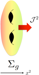
Figure 2: The BRST current $\mathcal{J}^{2}$ in the effective theory of the M2-branes wrapping $\Sigma_{g}$. The current is associated with the BRST charges defined on $\Sigma_{g}$. We require that it vanishes at the boundary.

Although there would be various solutions to the equation (3.1), we are interested in the solutions which correspond to the M2-M5-M5’ system (2.6). We can apply the general lesson we have learned in the flat case to find them. At the boundary of the M5-brane the bosonic one-form field $\Phi_{\alpha}$ should obey a particular boundary condition. However, the bosonic scalar fields $\phi^{I}$ should have two different types of boundary conditions due to the tangent and normal directions of the attached M5-brane. These are expected to be the Basu-Harvey like boundary condition describing a non-trivial geometry inside the M5-brane and the Dirichlet boundary condition respectively. Let $\phi^{\hat{i}}$, $\hat{i}=1,2$ be the scalar fields $\phi^{1}$ and $\phi^{2}$ which represent the position of the M2-branes within the M5-brane and let $\rho^{\hat{p}}$, $\hat{p}=1,\cdots,4$ be $\phi^{3}$, $\cdots$, $\phi^{6}$ which correspond to the transverse directions of the M5-brane. To obtain the Dirichlet condition on $\rho^{\hat{p}}$ we must require the fermionic boundary conditions

$$\overline{\xi}\hat{\Gamma}^{\hat{p}+4}\psi\Bigl{|}_{\textrm{bdy}} =0, \overline{\tilde{\xi}}\hat{\Gamma}^{\hat{p}+4}\tilde{\lambda}\Bigl{|}_{\textrm{bdy}} =0.$$ (3.33)

On the other hand, the Basu-Harvey type condition on $\phi^{\hat{i}}$ can be acquired by choosing the fermionic boundary conditions

$$\overline{\xi}\hat{\Gamma}^{\hat{i}+2}\Psi_{z}\Bigl{|}_{\textrm{bdy}} =0, \overline{\tilde{\xi}}\hat{\Gamma}^{\hat{i}+2}\tilde{\Psi}_{\overline{z}}\Bigl{|}_{\textrm{bdy}} =0.$$ (3.34)

The set of equations (3.33) and (3.34) states that the fermion bilinear forms cannot play the role of generators of translations in the corresponding directions.

Employing the fermionic boundary conditions (3.33) and (3.34), we can read off from the generic supersymmetric condition (3.1) the boundary conditions at the intersection of the M2-branes and the M5-brane in the brane configuration (2.6)

$$D_{2}\phi^{\hat{i}}-[\Phi_{z},\Phi_{\overline{z}},\phi^{\hat{i}}]\Bigl{|}_{\textrm{bdy}} =0,$$ (3.35)

$$D_{\overline{z}}\rho^{\hat{p}}\Bigl{|}_{\textrm{bdy}} =0,\ \ \ D_{z}\rho^{\hat{p}}\Bigl{|}_{\textrm{bdy}}=0,$$ (3.36)

$$D_{\overline{z}}\Phi_{z}\Bigl{|}_{\textrm{bdy}} =0,\ \ \ D_{z}\Phi_{\overline{z}}\Bigl{|}_{\textrm{bdy}}=0,$$ (3.37)

$$\overline{\xi}\left(D_{2}\Phi_{z}+\frac{1}{2}[\rho^{\hat{p}},\rho^{\hat{q}},\Phi_{z}]\hat{\Gamma}^{\hat{p}\hat{q}}\right)\tilde{\Psi}_{\overline{z}}\Bigl{|}_{\textrm{bdy}} =0,\ \ \ \overline{\tilde{\xi}}\left(D_{2}\Phi_{\overline{z}}+\frac{1}{2}[\rho^{\hat{p}},\rho^{\hat{q}},\Phi_{\overline{z}}]\hat{\Gamma}^{\hat{p}\hat{q}}\right)\Psi_{z}\Bigl{|}_{\textrm{bdy}}=0.$$ (3.38)

The equation (3.35) is the Basu-Harvey like equation on the scalars $\phi^{\hat{i}}$ and the set of equations (3.36) is the Dirichlet boundary condition on the scalars $\rho^{\hat{p}}$. Note that the set of equations (3.37) is not the Dirichlet boundary condition, but the holomorphic and anti-holomorphic boundary conditions on the one-form fields $\Phi_{z}$ and $\Phi_{\overline{z}}$ which are complex-valued functions on the Riemann surface $\Sigma_{g}$. Consequently $\Phi_{z}dz$ is a holomorphic differential one-form while $\Phi_{\overline{z}}d\overline{z}$ is an anti-holomorphic differential one-form on $\Sigma_{g}$. The field $\Phi_{z}$ satisfying equation (3.37) describes a choice of the holomorphic curve $\Sigma_{g}$ in K3.

Likewise we can find the boundary conditions at the M5’-brane by exchanging the pair of directions $(x^{3},x^{4})$ with $(x^{5},x^{6})$. Putting the M5’-brane in the M2-M5 configuration breaks down the space-time symmetry group $SO(4)_{3456}$ to $SO(2)_{34}\times SO(2)_{56}$ while it maintains the preserved supersymmetry, as we will see momentarily. Let $\varphi^{\hat{i}}$, $i=1,2$ be the bosonic scalars which correspond to the position of the M2-brane in the $(x^{3},x^{4})$, $\varsigma^{\hat{l}}$, $\hat{l}=1,2$ be those in the $(x^{5},x^{6})$ and $\varrho^{\hat{p}}$, $\hat{p}=1,2$ be those in the $(x^{7},x^{8})$. The first two, $\varphi^{\hat{i}}$ and $\varsigma^{\hat{l}}$ should obey the Basu-Harvey type condition as they probe in one of the fivebranes while the third $\varrho^{\hat{p}}$ must be subject to the Dirichlet condition. Now consider the limit in which the distance $L$ goes to zero, the intersection of the M2-M5-M5’ branes (2.6). The boundary conditions can be determined by combining the two types of conditions required from M5-brane and M5’-brane as

$$D_{2}\varphi^{\hat{i}}-[\Phi_{z},\Phi_{\overline{z}},\varphi^{\hat{i}}]\Bigl{|}_{\textrm{bdy}} =0, D_{z}\varphi^{\hat{i}}\Bigl{|}_{\textrm{bdy}} =0, D_{\overline{z}}\varphi^{\hat{i}}\Bigl{|}_{\textrm{bdy}} =0,$$ (3.39)

$$D_{2}\varsigma^{\hat{l}}-[\Phi_{z},\Phi_{\overline{z}},\varsigma^{\hat{l}}]\Bigl{|}_{\textrm{bdy}} =0, D_{z}\varsigma^{\hat{l}}\Bigl{|}_{\textrm{bdy}} =0, D_{\overline{z}}\varsigma^{\hat{l}}\Bigl{|}_{\textrm{bdy}} =0,$$ (3.40)

$$D_{z}\varrho^{\hat{p}}\Bigl{|}_{\textrm{bdy}} =0, D_{\overline{z}}\varrho^{\hat{p}}\Bigl{|}_{\textrm{bdy}} =0,$$ (3.41)

$$D_{2}\Phi_{z}+\frac{1}{2}[\varrho^{1},\varrho^{2},\Phi_{z}]\Bigl{|}_{\textrm{bdy}} =0, D_{\overline{z}}\Phi_{z}\Bigl{|}_{\textrm{bdy}} =0,$$ (3.42)

$$D_{2}\Phi_{\overline{}}+\frac{1}{2}[\varrho^{1},\varrho^{2},\Phi_{\overline{z}}]\Bigl{|}_{\textrm{bdy}} =0, D_{z}\Phi_{\overline{z}}\Bigl{|}_{\textrm{bdy}} =0.$$ (3.43)

We see that the two bosonic scalars $\varphi^{\hat{i}}$ and $\varsigma^{\hat{l}}$ are also subject to the Dirichlet conditions in equation (3.39) and equation (3.40) which are required by the other fivebrane. These conditions imply that they must be at fixed values so that they are the solutions to the Basu-Harvey type equations. Namely, the scalars $\varphi^{\hat{i}}$ and $\varsigma^{\hat{l}}$ obeying the boundary conditions (3.39) and (3.40) have neither non-trivial solutions nor divergent behaviour as they are fixed at one end or at the other end.

As we already explained, the conditions $D_{\overline{z}}\Phi_{z}=0$ and $D_{z}\Phi_{\overline{z}}=0$ in equations (3.42) and (3.43) are the holomorphic and anti-holomorphic conditions rather than the Dirichlet boundary conditions. So they cannot completely fix the complex-valued $\Phi_{z}$ and $\Phi_{\overline{z}}$, which may still satisfy the Basu-Harvey like conditions in equations (3.42) and (3.43). Also note that the solutions to the Basu-Harvey-like equations of the complex-valued one-forms do not have divergent behaviour as opposed to those of scalars with Nahm-like poles. Thus we expect that the bosonic degrees of freedom on the intersection of M2- and M5-branes inside the K3 can be effectively described by means of the bosonic one-form $\Phi_{\alpha}$ by taking an appropriate limit.

Since the M5-brane and the M5’-brane break the isometry of the flat directions as

$$SO(6)_{345678} \rightarrow SO(2)_{34}\times SO(4)_{5678}$$

$$\rightarrow SO(2)_{34}\times SO(2)_{56}\times SO(2)_{78}$$ (3.44)

via two projections, the 16 components of the fermionic fields in equation (2.14) reduce to a pair of complex fermionic scalar fields in holomorphic and anti-holomorphic sectors, which we will call $\theta$ and $\overline{\theta}$, and a pair of complex fermionic one-form fields in holomorphic and anti-holomorphic sectors, which we will call $p_{z}$ and $\overline{p}_{\overline{z}}$.

Here we want to pay special attention to the Basu-Harvey type supersymmetric boundary conditions in (3.39), (3.40), (3.42) and (3.43) because they provide for us a hint about the effective theory as a topological sigma model. Given the Basu-Harvey type equations as the boundary conditions, the 3-bracket structure can survive at the boundary and the Hermitian 3-algebra can be constructed by a pair $(\mathfrak{so}(4),V)$ where $V$ is a faithful orthogonal representation of the Lie algebra $\mathfrak{so}(4)$ equipped with a 3-bracket. Quite interestingly, it was shown in [21] that the Hermitian 3-algebra is generically embedded into a complex matrix Lie superalgebra $\mathfrak{sg}$ with an even subalgebra $\mathfrak{g}_{\mathbb{C}}$, the complexification of the corresponding Lie algebra $\mathfrak{g}$, and an odd subspace $V\oplus V^{*}$. In fact it has been pointed out more directly in [22] that the Basu-Harvey type equations are sufficient conditions to realize the Lie superalgebra. In general the Jacobi identity of a Lie superalgebra consists of four components corresponding to the relationship between three elements of the Lie superalgebra; even-even-even, even-even-odd, even-odd-odd and odd-odd-odd. Among them the only non-trivial piece is the odd-odd-odd Jacobi identity and the Basu-Harvey type equation guarantees the odd-odd-odd Jacobi identity. Hence the appearance of the Basu-Harvey equations in the supersymmetric boundary conditions indicates that the target space of the effective sigma model is a Lie superalgebra. As we will explicitly see later, it is the Lie superalgebra $\mathfrak{psl}(2|2)$ with even subalgebra $\mathfrak{sl}(2,\mathbb{C})\oplus\mathfrak{sl}(2,\mathbb{C})$.

3.2 Gauge invariant boundary conditions

So far we have determined the supersymmetric boundary conditions for the matter fields of the twisted BLG-model that would describe the M2-M5-M5’ system (2.6). However, we have not yet determined the boundary conditions for the gauge fields from supersymmetry because the supercurrent does not contain the field strength which demands the Neumann or the Dirichlet type boundary conditions for gauge fields. While there are many choices of boundary conditions for gauge fields, we are especially interested in those which keep a full gauge symmetry. Boundary conditions for the gauge field in ABJM theory have previously been studied in [23, 8, 12] and in [8] a boundary action was introduced which preserved the full gauge symmetry. However, here we will come up with an amazing result as a combination with the supersymmetric boundary conditions (3.39)-(3.43) on the twisted matter fields.

Since the twisted Chern-Simons term (2.9) whose variation produces a boundary term is not gauge invariant, we want to fix the boundary conditions for the gauge fields so that the gauge invariance of the bulk theory can be completely preserved . First, let us consider the pure Chern-Simons action. The variation of the Chern-Simons action

$$S_{\mathrm{CS}} =\frac{k}{4\pi}\int_{M}d^{3}x\epsilon^{\mu\nu\lambda}\mathrm{Tr}\left(A_{\mu}\partial_{\nu}A_{\lambda}+\frac{2i}{3}A_{\mu}A_{\nu}A_{\lambda}\right)$$ (3.45)

yields

$$\delta S_{\textrm{CS}} =\frac{k}{4\pi}\int_{M}d^{3}x\epsilon^{\mu\nu\lambda}\mathrm{Tr}\left(\delta A_{\mu}F_{\nu\lambda}\right)+\frac{k}{4\pi}\int_{\partial M}d^{2}x\epsilon^{\alpha\beta}\mathrm{Tr}\left(\delta A_{\alpha}A_{\beta}\right).$$ (3.46)

The second term does not automatically vanish on the boundary, but boundary conditions which set one of the components of the gauge field to zero at the boundary can be chosen to make the Chern-Simons action invariant under the gauge transformation. The effect of such boundary conditions is that the Chern-Simons action can be rearranged to show that the chosen component becomes a (bulk) Lagrange multiplier, enforcing the constraint that the field strength in the orthogonal directions vanishes [24]. For a Lorentzian two-dimensional boundary one can choose the time-like $A_{0}|_{\textrm{bdy}}=0$, space-like $A_{1}|_{\textrm{bdy}}=0$, or light-like $A_{\pm}$ $:=$ $A_{0}\pm A_{1}|_{\textrm{bdy}}=0$ boundary conditions. The choice of boundary conditions determines the form of the boundary kinetic term. For example, the light-like boundary condition $A_{+}|_{\textrm{bdy}}=0$ leads to the constraint $F_{2-}=0$ [8]. The Euclidean two-dimensional boundary that we are now considering can be realized by performing the Wick rotation. The light-like boundary conditions become a holomorphic boundary condition

$$A_{z}\Bigl{|}_{\textrm{bdy}}=\frac{1}{\sqrt{2}}\left(A_{0}-iA_{1}\right)\Bigl{|}_{\textrm{bdy}}=0$$ (3.47)

and an anti-holomorphic boundary condition

$$A_{\overline{z}}\Bigl{|}_{\textrm{bdy}}=\frac{1}{\sqrt{2}}\left(A_{0}+iA_{1}\right)\Bigl{|}_{\textrm{bdy}}=0,$$ (3.48)

which respectively yield the conditions

$$F_{2\overline{z}}=0$$ (3.49)

and

$$F_{2z}=0.$$ (3.50)

Now let us first assume for simplicity that this flatness condition can be solved as the pure gauge $A_{2}=g^{-1}\partial_{2}g$, $A_{z}=g^{-1}\partial_{z}g$ (or $A_{\overline{z}}=g^{-1}\partial_{\overline{z}}g$) where $g$ is a map from $\partial M=\Sigma$ at $x^{2}=0$ to the gauge group $G$, and the map is arbitrarily smoothly extended to $x^{2}>0$. Substituting into the action we find

$$S_{\textrm{CS}} =\frac{k}{4\pi}\int_{M}d^{3}x\mathrm{Tr}\left((g^{-1}\partial_{2}g)\partial_{z}(g^{-1}\partial_{\overline{z}}g)-(g^{-1}\partial_{\overline{z}}g)\partial_{z}(g^{-1}\partial_{2}g)\right)$$

$$=\frac{k}{4\pi}\int_{M}d^{3}x\mathrm{Tr}\Biggl{[}-(g^{-1}\partial_{2}g)(g^{-1}\partial_{z}g)(g^{-1}\partial_{\overline{z}}g)+(g^{-1}\partial_{\overline{z}}g)(g^{-1}\partial_{z}g)(g^{-1}\partial_{2}g)$$

$$+(g^{-1}\partial_{2}g)(g^{-1}\partial_{z}\partial_{-}g)-(g^{-1}\partial_{\overline{z}}g)(g^{-1}\partial_{z}\partial_{2}g)\Biggr{]}.$$ (3.51)

Now integrate by parts with respect to $\overline{z}$ in the first and $x^{2}$ in the second. Then the integration by parts with respect to $x^{2}$ produces the standard kinetic term on the boundary while the first does not produce a boundary term. All other terms from the last line cancel between the two terms so that we are left with the WZW-model

$$S_{\textrm{WZW}}= -\frac{k}{8\pi}\int_{\Sigma}d^{2}x\mathrm{Tr}\left(g^{-1}\partial_{\alpha}g\right)^{2}-\frac{ik}{12\pi}\int_{M}d^{3}x\epsilon^{\mu\nu\lambda}\mathrm{Tr}\left(g^{-1}\partial_{\mu}g\cdot g^{-1}\partial_{\nu}g\cdot g^{-1}\partial_{\lambda}g\right).$$ (3.52)

Back to the case of the BLG-model with a boundary, let us define $A_{\mu}=A_{\mu 4i}^{(+)}\sigma_{i}$ and $\hat{A}_{\mu}=A_{\mu 4i}^{(-)}\sigma_{i}$ where $A^{(+)}_{\mu 4i}$ and $A^{(-)}_{\mu 4i}$ are self-dual and anti-self-dual parts of the gauge fields and the Pauli matrices $\sigma_{i}$ are normalized as $\mathrm{Tr}(\sigma_{i}\sigma_{j})=2\delta_{ij}$. Then the twisted Chern-Simons term (2.9) in the BLG-model can be expressed as the $SU(2)_{k}$ $\times$ $SU(2)_{-k}$ quiver Chern-Simons term [25]

$$S_{\textrm{CS}} =\frac{k}{4\pi}\int_{M}d^{3}x\epsilon^{\mu\nu\lambda}\left[\mathrm{Tr}\left(A_{\mu}\partial_{\nu}A_{\lambda}+\frac{2i}{3}A_{\mu}A_{\nu}A_{\lambda}\right)-\mathrm{Tr}\left(\hat{A}_{\mu}\partial_{\nu}\hat{A}_{\lambda}+\frac{2i}{3}\hat{A}_{\mu}\hat{A}_{\nu}\hat{A}_{\lambda}\right)\right]$$ (3.53)

with $k\in\mathbb{Z}$. Let us choose the boundary conditions

$$A_{z}\Big{|}_{\textrm{bdy}} =0, \hat{A}_{z}\Big{|}_{\textrm{bdy}} =0,$$ (3.54)

which require that

$$F_{2\overline{z}} =0, \hat{F}_{2\overline{z}} =0.$$ (3.55)

From the quiver Chern-Simons action (3.53) we then find the boundary action

$$S_{\textrm{$SU(2)_{k}$WZW}}[g]+S_{\textrm{$SU(2)_{-k}$WZW}}[\hat{g}]$$

$$= -\frac{k}{8\pi}\int_{\Sigma}d^{2}x\mathrm{Tr}\left(g^{-1}\partial_{\alpha}g\right)^{2}-\frac{ik}{12\pi}\int_{M}d^{3}x\epsilon^{\mu\nu\lambda}\mathrm{Tr}\left(g^{-1}\partial_{\mu}g\cdot g^{-1}\partial_{\nu}g\cdot g^{-1}\partial_{\lambda}g\right)$$

$$+\frac{k}{8\pi}\int_{\Sigma}d^{2}x\mathrm{Tr}\left(\hat{g}^{-1}\partial_{\alpha}\hat{g}\right)^{2}+\frac{ik}{12\pi}\int_{M}d^{3}x\epsilon^{\mu\nu\lambda}\mathrm{Tr}\left(\hat{g}^{-1}\partial_{\mu}\hat{g}\cdot\hat{g}^{-1}\partial_{\nu}\hat{g}\cdot\hat{g}^{-1}\partial_{\lambda}\hat{g}\right).$$ (3.56)

In terms of $g$ and $\hat{g}$ the action (3.53) now becomes a sum of the two WZW actions. As discussed in [24], the measure is $\int[DA][D\hat{A}]\delta(F)\delta(\hat{F})$ $=\int[Dg][D\hat{g}]$ and there is no Jacobian in the change of variables.

Now, in general the flat condition cannot necessarily be solved by a single-valued function on a curve as $g:\Sigma_{g}\times\mathbb{R}\rightarrow SU(2)$. The conjugacy class of a non-trivial holonomy of a flat connection around sources would lead to additional boundary degrees of freedom as the coadjoint action in the effective action [26, 24]. However, even in the general case the WZW model would be part of the description, along with a contribution from the Chern-Simons action involving the non-trivial flat connections. As the moduli space of flat connections depends on the choice of $\Sigma_{g}$ it may be more convenient to use an alternative method to describe the Chern-Simons theory with a boundary. This involves adding new boundary degrees of freedom, coupled to the bulk Chern-Simons action, in such a way that gauge symmetry is preserved [27]. This approach has been used in the context of the ABJM model [8, 23]. In this approach it is clear that a WZW model will arise from the bulk gauge field on any manifold with a boundary, even though the full result including all ABJM matter fields and supersymmetry is not known even in the simplest case of $M=\mathbb{R}^{2}\times[0,L]$. For our purposes the appearance of the WZW model is the key point, and at least in the case of pure Chern-Simons theory the boundary conditions and boundary degrees of freedom approaches are equivalent.

4 Supergroup WZW Models

4.1 $PSL(2|2)$ WZW model and twisted BLG-model

4.1.1 Bosonic action

Now we wish to collect the bosonic boundary conditions – the supersymmetric boundary conditions (3.39)-(3.43) and the gauge invariant boundary conditions (3.54)-(3.55) – to explore the effective boundary theory on the two membranes in the M2-M5-M5’ system (2.6).

Let us introduce the complexified gauge fields

$${{\tilde{\mathcal{A}}_{z}\ }^{b}}_{a} ={{\tilde{A}_{z}\ }^{b}}_{a}+{f^{cdb}}_{a}\Phi_{\overline{z}c}\varphi^{*}_{d}+{f^{cdb}}_{a}\Phi_{\overline{z}c}\varsigma^{*}_{d}$$ (4.1)

$${{\tilde{\mathcal{A}}_{\overline{z}}\ }^{b}}_{a} ={{\tilde{A}_{\overline{z}}\ }^{b}}_{a}+{f^{cdb}}_{a}\Phi_{zc}\varphi_{d}+{f^{cdb}}_{a}\Phi_{zc}\varsigma_{d}$$ (4.2)

$${{\tilde{\mathcal{A}}_{2}\ }^{b}}_{a} ={{\tilde{A}_{2}\ }^{b}}_{a}+{f^{cdb}}_{a}\Phi_{\overline{z}c}\Phi_{zd}+{f^{cdb}}_{a}\varphi_{c}\varsigma_{d}+{f^{cdb}}_{a}\varrho_{c}\varrho^{*}_{d}$$ (4.3)

and the complexified field strength

$${\tilde{{\mathcal{F}}_{\mu\nu}}^{b}}_{a} =\partial_{\nu}{\tilde{{\mathcal{A}}_{\mu}}^{b}}_{a}-\partial_{\mu}{\tilde{{\mathcal{A}}_{\nu}}^{b}}_{a}-{\tilde{{\mathcal{A}}_{\mu}}^{b}}_{c}{\tilde{{\mathcal{A}}_{\nu}}^{c}}_{a}+{\tilde{{\mathcal{A}}_{\nu}}^{b}}_{c}{\tilde{{\mathcal{A}}_{\mu}}^{c}}_{a}$$ (4.4)

as well as the complexified scalars, e.g. $\varphi:=\frac{1}{\sqrt{2}}(\varphi^{1}-i\varphi^{2})$. Then by definition we have

$$\tilde{\mathcal{F}}_{2\overline{z}} =\tilde{F}_{2\overline{z}}-\left[D_{2}\Phi_{z}+\frac{1}{2}[\varrho,\varrho^{*},\Phi_{z}],\varphi,\ \right]-\left[D_{2}\Phi_{z}+\frac{1}{2}[\varrho,\varrho^{*},\Phi_{z}],\varsigma,\ \right]$$

$$-\Bigl{[}\Phi_{z},D_{2}\varphi-[\Phi_{\overline{z}},\Phi_{\overline{z}},\varphi],\ \Bigr{]}-\Bigl{[}\Phi_{\overline{z}},D_{2}\varsigma-[\Phi_{z},\Phi_{\overline{z}},\varsigma],\ \Bigr{]}$$

$$+\Bigl{[}D_{\overline{z}}\Phi_{\overline{z}},\Phi_{z},\ \Bigr{]}+\Bigl{[}\Phi_{\overline{z}},D_{\overline{z}}\Phi_{z},\ \Bigr{]}+\Bigl{[}D_{\overline{z}}\varphi,\varsigma,\ \Bigr{]}+\Bigl{[}\varphi,D_{\overline{z}}\varsigma,\ \Bigr{]}$$

$$+\Bigl{[}D_{\overline{z}}\varrho,\varrho^{*},\ \Bigr{]}+\Bigl{[}\varrho,D_{\overline{z}}\varrho^{*},\ \Bigr{]}.$$ (4.5)

Therefore both the supersymmetric boundary conditions (3.39)-(3.43) and the gauge invariant boundary conditions (3.54)-(3.55) can be unified as an equation

$$\tilde{\mathcal{F}}_{2\overline{z}} =0$$ (4.6)

in terms of the complexified field strength (4.4).

It is remarkable that such a complexification of the gauge field and the simplification of the BPS equation are also encountered in the case of wrapped D3-branes on a holomorphic curve $\Sigma_{g}$ in K3 (see e.g. [11, 28]). In that case the effective theory can be described by the four-dimensional twisted $\mathcal{N}=4$ super Yang-Mills theory on $\Sigma_{g}$. A set of BPS equations on $\Sigma_{g}$ for $g>1$ is known to be Hitchin’s equations; $F_{z\overline{z}}+i[\Phi_{z},\Phi_{\overline{z}}]=0$, $D_{z}\Phi_{\overline{z}}=0$ and $D_{\overline{z}}\Phi_{z}=0$. They can be summarized as the condition $\mathcal{F}_{z\overline{z}}=0$, which is the flatness condition on the complexified gauge field $\mathcal{A}_{z}:=A_{z}-i\Phi_{z}$. Moreover, the equation (4.6) reflects the fact that existence of high amounts of supersymmetry in Chern-Simons matter theories is inseparably bound up with gauge symmetry.

In trying to find the effective action of the boundary theory, we demand that it is classically scale invariant on the two-dimensional boundary $\Sigma_{g}$. To seek such a Lagrangian description, it is instructive to look at the bosonic action of the fully topologically twisted BLG-model on a general compact three-manifold $M$ [29]

$$S_{\textrm{bosonic TBLG}}=\int_{M}d^{3}x \left[\frac{i}{2}\epsilon^{\mu\nu\lambda}\left(f^{abcd}\bm{\mathcal{A}}_{\mu ab}\partial_{\nu}\bm{\mathcal{A}}_{\lambda cd}+\frac{2}{3}{f^{cda}}_{g}f^{efgb}\bm{\mathcal{A}}_{\mu ab}\bm{\mathcal{A}}_{\nu cd}\bm{\mathcal{A}}_{\lambda ef}\right)\right]$$

$$+\sqrt{g}\mathrm{Tr}\Biggl{[}\frac{1}{2}\left(\bm{\mathcal{D}}^{\mu}\bm{\Phi}_{\mu}-\frac{i}{3\sqrt{g}}\epsilon^{\mu\nu\lambda}[\bm{\Phi}_{\mu},\bm{\Phi}_{\nu},\bm{\Phi}_{\lambda}]\right)^{2}$$

$$+\frac{1}{4}\left(\bm{\mathcal{D}}_{\mu}\bm{\Phi}_{\nu}-\bm{\mathcal{D}}_{\nu}\bm{\Phi}_{\mu}\right)\left(\bm{\mathcal{D}}^{\mu}\bm{\Phi}^{\nu}-\bm{\mathcal{D}}^{\nu}\bm{\Phi}^{\mu}\right)$$

$$+\frac{1}{2}\bm{\mathcal{D}}^{\mu}\bm{\phi}^{I}\bm{\mathcal{D}}_{\mu}\bm{\phi}^{I}+\frac{1}{12}[\bm{\phi}^{I},\bm{\phi}^{J},\bm{\phi}^{K}][\bm{\phi}^{I},\bm{\phi}^{J},\bm{\phi}^{K}]$$

$$+\frac{1}{4}[\bm{\Phi}_{\mu},\bm{\phi}^{I},\bm{\phi}^{J}][\bm{\Phi}^{\mu},\bm{\phi}^{I},\bm{\phi}^{J}]\Biggr{]}$$ (4.7)

where

$$\bm{\mathcal{A}}_{\mu ab} =A_{\mu ab}-\frac{i}{2\sqrt{g}}\epsilon_{\mu\nu\lambda}{f^{cd}}_{ab}\bm{\Phi}^{\nu}_{c}\bm{\Phi}_{d}^{\lambda},$$ (4.8)

$$(\bm{\mathcal{D}}_{\mu}X)_{a} =\partial_{\mu}X_{a}-{\bm{\mathcal{A}}_{\mu}}^{b}\ _{a}X_{b}$$

$$=(D_{\mu}X)_{a}+\frac{i}{2\sqrt{g}}\epsilon_{\mu\nu\lambda}[\bm{\Phi}^{\nu},\bm{\Phi}^{\lambda},X]_{a}$$ (4.9)

are the three-dimensional versions of complexified objects while $\bm{\Phi}_{\mu}$ and $\bm{\phi}^{I}$ are component fields of the bosonic $SO(3)$ one-form field and the five bosonic scalar fields respectively.

However, for the partially twisted BLG-model on $\Sigma_{g}$ together with boundaries, the complexification comes about in a slightly different way from (4.8) and (4.1.1) according to the breakdown of the rotational symmetry; $SO(3)\rightarrow SO(2)$. This allows the complexified scalar fields to enter the complexification as in (4.1)-(4.3). Note that the $x^{2}$ component of the complexified gauge fields, $\mathcal{A}_{2}$ is now identified with a bosonic scalar field and contains additional contributions from complexified scalar fields in our definition (4.3). Furthermore the partially twisted action takes a different form in terms of the modified complexified gauge fields (4.1)-(4.3). In the fully twisted action (4.1.1) there are four types of classically scale invariant terms on a Riemann surface $\Sigma_{g}$ which can contribute to the effective boundary action;

1. the twisted Chern-Simons term of the complexified gauge fields in the first line,

2. the quadratic term $(D_{2}\Phi_{\alpha}-D_{\alpha}\phi)^{2}$ with $\phi$ being the bosonic scalar fields in the third line,

3. the kinetic terms $(D_{\alpha}\phi)^{2}$ of the bosonic scalar fields in the fourth line,

4. the potential terms of the form $[\Phi_{\alpha},\phi,\phi]^{2}$ in the fifth line.

Now we point out that under the supersymmetric boundary conditions (3.39)-(3.43) which are encoded by the complexified gauge fields (4.1)-(4.3) as equation (4.6), all the possible terms (i)-(iv) can be formally collected as the twisted Chern-Simons term

$$S_{\textrm{bosonic TBLG}} =\int_{\Sigma_{g}\times I}d^{3}x\left[\frac{1}{2}\epsilon^{\mu\nu\lambda}\left(f^{abcd}\mathcal{A}_{\mu ab}\partial_{\nu}\mathcal{A}_{\lambda cd}+\frac{2}{3}{f^{cda}}_{g}f^{efgb}\mathcal{A}_{\mu ab}\mathcal{A}_{\nu cd}\mathcal{A}_{\lambda ef}\right)\right]$$ (4.10)

of the complexified gauge fields (4.1)-(4.3). This implements the complexification of the twisted Chern-Simons term (2.9). One can therefore view the supersymmetric boundary conditions (3.39)-(3.43) and the gauge invariant boundary conditions (3.54)-(3.55) as the complexified gauge invariant boundary condition (4.6) in the twisted Chern-Simons term (4.10). Following the previous logic, we can now get the bosonic boundary action.

The twisted Chern-Simons term (2.9) can be rewritten as a sum of two Chern-Simons actions as in (3.53). With the aid of the gauge invariant boundary conditions (3.54) they give rise to a sum of two WZW actions (3.2), although as previously discussed we cannot exclude additional contributions from non-trivial flat connections. Thus the twisted Chern-Simons term (4.10) of the complexified gauge fields $\mathcal{A}_{\mu}$ with the boundary condition (4.6) generates the boundary action as a sum of two $SL(2,\mathbb{C})$ WZW actions

$$S_{\textrm{bosonic}}= S_{\textrm{$SL(2,\mathbb{C})_{k}$WZW}}[g]+S_{\textrm{$SL(2,\mathbb{C})_{-k}$WZW}}[\hat{g}]$$

$$= -\frac{k}{8\pi}\int_{\Sigma_{g}}d^{2}x\mathrm{Tr}\left(g^{-1}\partial_{\alpha}g\right)^{2}-\frac{ik}{12\pi}\int_{M}d^{3}x\epsilon^{\mu\nu\lambda}\mathrm{Tr}\left(g^{-1}\partial_{\mu}g\cdot g^{-1}\partial_{\nu}g\cdot g^{-1}\partial_{\lambda}g\right)$$

$$+\frac{k}{8\pi}\int_{\Sigma_{g}}d^{2}x\mathrm{Tr}\left(\hat{g}^{-1}\partial_{\alpha}\hat{g}\right)^{2}+\frac{ik}{12\pi}\int_{M}d^{3}x\epsilon^{\mu\nu\lambda}\mathrm{Tr}\left(\hat{g}^{-1}\partial_{\mu}\hat{g}\cdot\hat{g}^{-1}\partial_{\nu}\hat{g}\cdot\hat{g}^{-1}\partial_{\lambda}\hat{g}\right).$$ (4.11)

4.1.2 Including fermionic terms

As discussed at the end of section 3.1, on general grounds we expect to have a supergroup structure. Obviously the natural expectation is that including the fermionic fields will enhance the $SL(2)\times SL(2)$ WZW model to a $PSL(2|2)$ WZW model. We will first review the form of the $PSL(2|2)$ WZW action [30, 31, 32] and then discuss how this can arise from the twisted Chern-Simons theory with our fermionic field content.

Let us begin by considering the $SL(2|2)$ WZW-model

$$S_{SL(2|2)_{k}}[s]=-\frac{k}{8\pi}\int_{\Sigma_{g}}d^{2}x\mathrm{Str}\left(s^{-1}\partial_{\alpha}s\right)^{2}-\frac{ik}{12\pi}\int_{M}d^{3}x\epsilon^{\mu\nu\lambda}\mathrm{Str}\left(s^{-1}\partial_{\mu}s\cdot s^{-1}\partial_{\nu}s\cdot s^{-1}\partial_{\lambda}s\right)$$ (4.12)

for supermatrices

$$s =\left(\begin{array}[]{cc}A&B\\ C&D\\ \end{array}\right)\in SL(2|2)$$ (4.15)

with $A$ and $D$ being bosonic matrix elements of $SL(2,\mathbb{C})$ and $B$ and $C$ being fermionic matrix elements. Here a supertrace $\mathrm{Str}$ is defined as $\mathrm{Str}(s)=\mathrm{Tr}(A)-\mathrm{Tr}(D)$. The supergroup element $s\in SL(2|2)$ admits the Gauss decomposition [33]

$$s =\exp(u)\left(\begin{array}[]{cc}\mathbb{I}&0\\ \overline{\theta}&\mathbb{I}\\ \end{array}\right)\left(\begin{array}[]{cc}g&0\\ 0&\hat{g}\\ \end{array}\right)\left(\begin{array}[]{cc}\mathbb{I}&\theta\\ 0&\mathbb{I}\\ \end{array}\right)$$ (4.22)

$$=\exp(u)\left(\begin{array}[]{cc}g&g\theta\\ \overline{\theta}g&\overline{\theta}g\theta+\hat{g}\\ \end{array}\right)$$ (4.25)

with $u\in\mathbb{C}$ and $g,\hat{g}$ $\in SL(2,\mathbb{C})$. The action (4.12) satisfies the Polyakov-Wiegmann identity [34]

$$S[s_{1}s_{2}] =S[s_{1}]+S[s_{2}]+\frac{k}{2\pi}\int d^{2}x\mathrm{Str}\left(s^{-1}_{1}\partial_{\overline{z}}s_{1}\partial_{z}s_{2}s_{2}^{-1}\right).$$ (4.26)

Now, $SL(2|2)$ has a normal $U(1)$ subgroup consisting of multiples of the identity. As discussed e.g. in [32] the $SL(2|2)$-invariant metric is degenerate. However, treating the U(1) symmetry as a gauge symmetry and quotienting by this U(1) results in a $PSL(2|2)$ WZW model, with a non-degenerate invariant metric. Since $PSL(2|2)$ has bosonic subgroup $SL(2)\times SL(2)$ this also gives the minimal embedding of the bosonic $SL(2)\times SL(2)$ WZW model into a supergroup WZW model.

Although $PSL(2|2)$ has no representation of supermatrices, one can descend to $PSL(2|2)$ from $SL(2|2)$ by identifying supermatrices $s\in SL(2|2)$ which differ by a scalar multiple. Using the Polyakov-Wiegmann identity (4.26) we can show that

$$S_{SL(2|2)_{k}}[e^{u}s] =S_{SL(2|2)}[e^{u}]+S_{SL(2|2)_{k}}[s]+\frac{k}{2\pi}\int_{\Sigma_{g}}d^{2}x\partial_{\overline{z}}u\mathrm{Str}(s\partial_{z}s^{-1})$$

$$=S_{SL(2|2)_{k}}[s].$$ (4.27)

This states that the action (4.12) is invariant after multiplying the supermatrices $s\in SL(2|2)$ with a scalar factor $\exp(u)$. In other words, the $PSL(2|2)$ WZW action is equivalent to the $SL(2|2)$ WZW action.

Applying the Polyakov-Wiegmann identity (4.26) to the decomposition (4.22) one can rewrite the $PSL(2|2)$ WZW model (4.12) as

$$S_{PSL(2|2)_{k}}[s] =S_{PSL(2|2)_{k}}\left[\left(\begin{array}[]{cc}\mathbb{I}&0\\ \overline{\theta}&\mathbb{I}\\ \end{array}\right)\right]+S_{PSL(2|2)_{k}}\left[\left(\begin{array}[]{cc}g&0\\ 0&\hat{g}\\ \end{array}\right)\right]+S_{PSL(2|2)_{k}}\left[\left(\begin{array}[]{cc}\mathbb{I}&\theta\\ 0&\mathbb{I}\\ \end{array}\right)\right]$$ (4.34)

$$+\frac{k}{2\pi}\int_{\Sigma_{g}}d^{2}x\mathrm{Str}\left(\begin{array}[]{cc}0&g^{-1}\partial_{\overline{z}}g\partial_{z}\theta\\ \partial_{\overline{z}}\overline{\theta}(\partial_{z}g)g^{-1}&\hat{g}^{-1}\partial_{\overline{z}}\overline{\theta}g\partial_{z}\theta\\ \end{array}\right).$$ (4.37)

The first and third terms vanish because contributions to supertraces can arise only from non-trivial bosonic submatrices. Then the final result is

$$S_{PSL(2|2)_{k}}[s] =S_{SL(2,\mathbb{C})_{k}\textrm{WZW}}[g]+S_{SL(2,\mathbb{C})_{-k}\textrm{WZW}}[\hat{g}]$$

$$-\frac{k}{2\pi}\int_{\Sigma_{g}}d^{2}x\mathrm{Tr}\left(\hat{g}^{-1}\partial_{\overline{z}}\overline{\theta}g\partial_{z}\theta\right).$$ (4.38)

The first two terms are the sum of two $SL(2,\mathbb{C})$ WZW models which we have encountered in the bosonic boundary action in (4.1.1). Notice that the opposite level comes from the definition of the supertrace.

Let us now proceed to discuss how this supergroup WZW model can arise from the fermionic degrees of freedom we have. Recall that the supersymmetric boundary conditions in the topologically twisted BLG model allow for the spin-zero fermionic fields $\theta$, $\overline{\theta}$ and spin-one fermionic fields $p_{z}$, $\overline{p}_{\overline{z}}$. We identify $\theta$, $\overline{\theta}$ with the fermionic fields in the supergroup WZW model. There could be a field redefinition in this relation, but this would just correspond to a different parametrisation of the supergroup elements. However, we note that the supergroup action does not include the fields $p_{z}$, $\overline{p}_{\overline{z}}$.

In constructing the boundary action with fermionic terms, we again demand that the possible boundary terms are scale invariant at the classical level. In two dimensions, the spin-zero and spin-one fermionic fields have scaling dimensions zero and one respectively. Without the couplings of the fermions to the bosons, one can write a conformally invariant action [35]

$$S =\frac{1}{\pi}\int d^{2}x\left(p_{z}\partial_{\overline{z}}\overline{\theta}+\overline{p}_{\overline{z}}\partial_{z}\theta\right).$$ (4.39)

This is the fermionic ghost system with central charge $c=-2$, the so-called symplectic fermions [9]. However, we should consider other possible terms which stem from the terms in the twisted BLG theory, i.e. the fermionic kinetic term $\left(\overline{\Psi},\Gamma^{\mu}D_{\mu}\Psi\right)$ and the interaction term $\left(\overline{\Psi},\Gamma^{IJ}[X^{I},X^{J},\Psi]\right)$. This means that the boundary terms are quadratic in fermionic fields, with up to one derivative acting on the fermions, and that they can also contain the bosonic matrix fields $g$, $\hat{g}$ and their inverses $g^{-1}$, $\hat{g}^{-1}$ of $SL(2,\mathbb{C})$. Taking into account the scale invariance, we could have the following possible boundary terms including the fermionic fields; $\theta$, $\overline{\theta}$, $p_{z}$, $\overline{p}_{\overline{z}}$, and the bosonic fields; $g$, $\hat{g}$, $g^{-1}$, $\hat{g}^{-1}$:

1. terms involving two fermionic scalar fields and no fermionic one-form field

   $$\partial_{z}\theta\hat{g}^{-1}\partial_{\overline{z}}\overline{\theta}g,\ \ \ \ \ \partial_{z}\theta\hat{g}\partial_{\overline{z}}\overline{\theta}g^{-1},$$ (4.40)

2. terms involving a fermionic scalar field and a fermionic one-form field

   $$p_{z}\hat{g}^{-1}\partial_{\overline{z}}\overline{\theta}g,\ \ \ \ \ \overline{p}_{\overline{z}}\hat{g}\partial_{z}\theta g^{-1},$$ (4.41)

3. terms involving no fermionic scalar field and two fermionic one-form fields

   $$p_{z}\hat{g}^{-1}\overline{p}_{\overline{z}}g,\ \ \ \ \ p_{z}\hat{g}\overline{p}_{\overline{z}}g^{-1}.$$ (4.42)

Now, the terms in (4.40) have two derivatives and do not obviously arise from the fermionic terms in the BLG theory. However, we note that the fermionic one-form fields $p_{z}$, $\overline{p}_{\overline{z}}$ have no kinetic terms and they therefore should be treated as auxiliary fields. After integrating them out we are expected to be left with the terms as in (4.40) which only contain the fermionic scalar fields $\theta$, $\overline{\theta}$. Thus the fermionic boundary degrees of freedom can be encoded in the interaction term

$$S_{\textrm{int}} =\int_{\Sigma_{g}}d^{2}x\mathrm{Tr}\left(\kappa_{A}\partial_{z}\theta\hat{g}^{-1}\partial_{\overline{z}}\overline{\theta}g+\kappa_{B}\partial_{z}\theta\hat{g}\partial_{\overline{z}}\overline{\theta}g^{-1}\right)$$ (4.43)

where $\kappa_{A}$ and $\kappa_{B}$ are constants.

Note that we didn’t directly derive the fermionic action from the twisted BLG action. In fact, since $g$ and $\hat{g}$ are dimensionless, it is consistent with dimensional analysis that there could be a variety of terms with $(\partial_{z}\theta)(\partial_{\overline{z}}\overline{\theta})$ in the final fermionic boundary action. Likewise the precise form of the coupling to $g$ and $\hat{g}$ may seem somewhat arbitrary. However, we would expect the requirement of conformal invariance (at the quantum level) to be highly restrictive. As we have seen above, including the above fermionic terms with $\kappa_{A}=-\frac{k}{2\pi}$, $\kappa_{B}=0$ gives the $PSL(2|2)$ WZW model, so this is certainly consistent with all our requirements for the action.

One plausible argument to constrain the allowed fermionic terms is to note that the bosonic WZW action has the obvious global symmetry

$$g\rightarrow ugv^{-1}\;,\;\;\;\hat{g}\rightarrow\hat{u}\hat{g}\hat{v}^{-1}.$$

If we assume the classical action has this symmetry when we include the fermions, we must assign specific transformation properties to the fermions or they could not couple to the bosonic fields. As the bulk fermions were in the bifundamental representation, we likewise expect the boundary fermions to allow coupling of $g$ to $\hat{g}$. In order for this to be possible we take the following transformation rules:

$$\theta\rightarrow v\theta\hat{v}^{-1} \overline{\theta}\rightarrow\hat{u}\overline{\theta}u^{-1},$$ , (4.44)

$$p_{z}\rightarrow vp_{z}\hat{v}^{-1} \overline{p}_{\overline{z}}\rightarrow\hat{u}\overline{p}_{\overline{z}}u^{-1}.$$ , (4.45)

Similar transformation rules are possible with different choices of $u\leftrightarrow v$ or $\hat{u}\leftrightarrow\hat{v}$ but these just differ by field redefinitions, by multiplying the fermions on the left or right by $g$, $\hat{g}$ or their inverses. With this particular convention we see that only the first term in (4.42) is allowed while both terms in (4.41) are possible. If these three terms are all present in the action then integrating out $p_{z}$ will produce exactly (4.43) with $\kappa_{B}=0$ and the non-zero value of $\kappa_{A}$ will just correspond to the normalisation of $\theta$ and $\overline{\theta}$. Even assuming the global symmetry, this argument is not quite complete as there are possible terms similar to those in (4.41) where the derivative acts on $g$ or $\hat{g}$. Allowing all such terms will generate several additional terms after integrating out $p_{z}$, e.g. $g^{-1}\partial g\theta\hat{g}^{-1}\overline{\partial}\overline{\theta}$. However, as far as we are aware, such possible fermionic couplings do not give rise to a CFT, so the requirement of conformal invariance will not allow such terms.

While we have not given a rigorous derivation, we believe that this is the unique result arising from the topologically twisted BLG-model on $\Sigma_{g}$ by choosing the supersymmetric and gauge invariant boundary conditions. Indeed, from the form of the bosonic part of the action, and the requirement of a supergroup structure, this is essentially the only possibility (other than adding additional fields which do not arise from the bulk theory.) If we simply demand conformal invariance, it is possible that other fermionic interactions are allowed. However, we are not aware of any such models with the same bosonic action (and where the fermions are coupled to the bosonic fields.) We do note that there is the interesting possibility discussed in [32] that there is a family of $PSL(N|N)$ WZW models which are conformal even when the coefficients of the kinetic term and the WZW term are independent. We have only discussed the case with the standard relation between these coefficients as that is what we expect to get from the Chern-Simons theory. However, it would be interesting to understand what role, if any, such deformations have in this context.

To summarise, we have obtained the $PSL(2|2)$ WZW model from the topologically twisted BLG-model on $\Sigma_{g}$ by choosing the supersymmetric and gauge invariant boundary conditions. In view of the form of the action (4.1.2), we see that a heuristic construction of highly supersymmetric conformally invariant gauge theories in three dimensions as the quiver Chern-Simons matter theories with opposite integer levels is intimately related to the structure of the supergroup WZW actions underlying the supertrace. Due to the wrong sign of the kinetic term, we do not expect this to be a unitary theory or even to directly arise from one by an analytic continuation. So one could not extract the dynamical properties of the M2-branes. However, the theory we are now considering is the effective field theory on the Euclidean $\Sigma_{g}$ wrapped by the M2-branes. The resulting theory, which is different from the original physical theory via topological twisting, could only capture the topological properties, or the BPS spectrum of the curved M2-branes wrapping a holomorphic Riemann surface $\Sigma_{g}$ as a topological field theory. We expect that it can play a similar role as other proposed effective theories arising from curved world-volumes of branes, e.g., two-dimensional topological sigma models for wrapped D3-branes on Riemann surfaces in K3 [11], $SL(2,\mathbb{C})$ Chern-Simons theory for wrapped M5-branes on 3-manifolds in Calabi-Yau three-folds [36], Vafa-Witten theory for wrapped M5-branes on 4-manifolds in $G_{2}$ manifolds [37]. Indeed the supergroup WZW-model is known to be a topological sigma model [33, 32] and also has been used to compute the Alexander polynomials $\Delta$ [38]. Remarkably it has been proven in [39] that any A-polynomials which occur as the Alexander polynomials can occur as the Seiberg-Witten invariant of an irreducible homotopy K3. We expect to be able to address these relations with our physical setup. In particular, for the effective theory of the topological M-strings in the brane configuration (2.6), the level would be $k=1$ since only it can realize two flat M2-branes in a flat space. Therefore we propose the $PSL(2|2)$ WZW model with level $k=1$ as the effective action of the two topological M-strings.

4.2 $GL(N|N)$ WZW model and twisted ABJM-model

Let us generalize our discussion to the case of an arbitrary number of coincident M2-branes in the brane configuration (2.6). The ABJM-model [6], which is a three-dimensional $\mathcal{N}=6$ superconformal $U(N)_{k}\times U(N)_{-k}$ Chern-Simons matter theory has been proposed as the low-energy world-volume effective theory of $N$ M2-branes probing $\mathbb{C}^{4}/\mathbb{Z}_{k}$. The theory involves four complex scalar fields $Y^{A}$, four Weyl spinor fields $\psi_{A}$ and two types of gauge fields $A_{\mu},\hat{A}_{\mu}$. The theory has $SU(4)_{R}$ R-symmetry group as well as $U(1)_{B}$ flavor symmetry group. $Y^{A}$ and $\psi_{A}$ are the matter fields transforming as the $(\bm{N},\overline{\bm{N}})$ bi-fundamental representation of the $U(N)_{k}\times U(N)_{-k}$ gauge group with $U(1)_{B}$ charge $+1$, while $Y_{A}^{{\dagger}}$ and $\psi^{{\dagger}A}$ are those transforming as the $(\overline{\bm{N}},\bm{N})$ anti-bi-fundamental representation with $U(1)_{B}$ charge $-1$. The upper and lower indices $A,B,\cdots=1,2,3,4$ correspond to the $\bm{4}$ and $\overline{\bm{4}}$ of the $SU(4)_{R}$ R-symmetry and baryonic charges $1$ and $-1$ respectively, while $A_{\mu}$ are the $U(N)$ Chern-Simons gauge fields of level $+k$ and $\hat{A}_{\mu}$ are the $U(N)$ Chern-Simons gauge fields of level $-k$. The gauge fields transform as the trivial representation of $SU(4)_{R}$ $\times$ $U(1)_{B}$.

If we try to get the low-energy effective theory of $N$ topological M-strings by carrying out the topological twist on the ABJM-model, it is necessary to consider the effect of the $U(1)_{B}$ charge. The global symmetry $SU(4)_{R}\times U(1)_{B}$ has 16 currents. However, when $k=1,2$ the monopole operators provide us with 12 symmetry generators so that the global symmetry is enhanced to $SO(8)_{R}$ with 28 generators. Thus the $\mathcal{N}=6$ supersymmetry of the ABJM-model is expected to be enhanced to $\mathcal{N}=8$ for $k=1$ and $k=2$ by taking into account the baryon symmetry $U(1)_{B}$ [6, 40, 41]. As discussed in [42], a topological twisting procedure generically can be regarded as a gauging of an internal symmetry group by adding to the original action the coupling of the internal current to the spin connection and one can also take such an internal symmetry as a baryon symmetry.

Now we attempt to twist the ABJM-model by first decomposing the R-symmetry as

$$SU(4)_{R}\rightarrow SU(3)_{R}\times U(1)_{R}.$$ (4.46)

Then we define a generator $\mathfrak{s}^{\prime}$ of the $SO(2)_{E}^{\prime}$ as

$$\mathfrak{s}^{\prime} =\mathfrak{s}-\frac{1}{2}T_{R}-\frac{1}{2}T_{B}$$ (4.47)

where $\mathfrak{s}$ is a generator of the original rotational group $SO(2)_{E}$, $T_{R}$ is a generator of $U(1)_{R}$ and $T_{B}$ is a generator of $U(1)_{B}$. The branching of the representation for the decomposition $SU(4)_{R}$ $\rightarrow$ $SU(3)_{R}\times U(1)_{R}$ is

$$\bm{6} \rightarrow\bm{3}_{2}\oplus\overline{\bm{3}}_{-2}$$

$$\bm{4} \rightarrow\bm{3}_{-}\oplus\bm{1}_{3}$$

$$\overline{\bm{4}} \rightarrow\overline{\bm{3}}_{+}\oplus\bm{1}_{-3}.$$ (4.48)

The twisting $SO(2)_{E}\times SU(4)_{R}\times U(1)_{B}$ $\rightarrow$ $SO(2)_{E}^{\prime}\times SU(3)_{R}$ reduces the supersymmetry parameter $\omega$ as follows:

$$\omega :\ \ \ \bm{6}_{+}\oplus\bm{6}_{-}\rightarrow\bm{3}_{0}\oplus\bm{3}_{2}\oplus\overline{\bm{3}}_{-2}\oplus\overline{\bm{3}}_{0}.$$ (4.49)

The appearance of the six covariantly constant spinors indicates that the twisting procedure corresponds to the M-theory background (2.1) since K3 breaks half of the supersymmetry. After the twisting $SO(2)_{E}\times SU(4)_{R}\times U(1)_{B}$ $\rightarrow$ $SO(2)_{E}^{\prime}\times SU(3)_{R}$, the fields transform as

$$Y^{A} :\ \ \ \bm{4}_{0}\rightarrow\bm{3}_{0}\oplus\bm{1}_{-2}$$

$$Y_{A}^{{\dagger}} :\ \ \ \overline{\bm{4}}_{0}\rightarrow\overline{\bm{3}}_{0}\oplus\bm{1}_{2}$$

$$\psi_{A} :\ \ \ \overline{\bm{4}}_{+}\oplus\overline{\bm{4}}_{-}\rightarrow\overline{\bm{3}}_{0}\oplus\bm{1}_{2}\oplus\overline{\bm{3}}_{-2}\oplus\bm{1}_{0}$$

$$\psi^{{\dagger}A} :\ \ \ \bm{4}_{+}\oplus\bm{4}_{-}\rightarrow\bm{3}_{2}\oplus\bm{1}_{0}\oplus\bm{3}_{0}\oplus\bm{1}_{-2}.$$ (4.50)

We see that the twisted ABJM-model comprises scalar fields $\bm{3}_{0}\oplus\overline{\bm{3}}_{0}$ with six components, bosonic one forms $\bm{1}_{2}\oplus\bm{1}_{-2}$ giving two components, fermionic scalar fields $\bm{3}_{0}\oplus\bm{1}_{0}$ $\oplus\overline{\bm{3}}_{0}\oplus\bm{1}_{0}$ with eight components and another eight components from fermionic one-form fields $\bm{1}_{2}\oplus\bm{3}_{2}$ $\oplus$ $\bm{1}_{-2}\oplus\overline{\bm{3}}_{-2}$. In other words, the twisted ABJM theory has exactly the same number of bosonic and fermionic field components as (2.13) and (2.14) in the twisted BLG theory. By imposing the appropriate supersymmetric boundary conditions on these fields, we find holomorphic, anti-holomorphic fermionic scalars $\theta$, $\overline{\theta}$ as well as fermionic one-form fields $p_{z}$, $\overline{p}_{\overline{z}}$. Therefore we are led to regard the above twisted theories as the source of the low-energy effective description of $N$ topological M-strings.

Since the twisting requires gauging both the $U(1)_{R}$ and $U(1)_{B}$ symmetries, a straightforward decomposition of gamma matrices and spinors cannot work. However, we would like to make a few remarks on the effective theory. First, the $U(N)\times U(N)$ Chern-Simons action should produce a sum of the two WZW actions with the holomorphic boundary conditions $A_{z}\bigl{|}_{\textrm{bdy}}=0$, $\hat{A}_{z}\bigl{|}_{\textrm{bdy}}=0$ as in (3.54) and (3.55) since the topological twisting does not affect the gauge fields and the Chern-Simons action. Second, the ABJM-model is shown to be written in terms of the 3-algebra [43], which enables us to define complexified gauge fields as in (4.1)-(4.3). This would promote the $U(N)\times U(N)$ gauge fields to the complexified $GL(N)\times GL(N)$ gauge fields. Third, the ABJM-model has the BPS boundary conditions for the bosonic scalar fields analogous to the Basu-Harvey equations which may represent $N$ M2-branes ending on the M5-brane [44]. It has been also argued in [22] that these are sufficient conditions for the presence of the Lie superalgebra $\mathfrak{gl}(N|N)$ with even subalgebra $\mathfrak{gl}(N,\mathbb{C})$ $\oplus$ $\mathfrak{gl}(N,\mathbb{C})$. Finally, the symplectic fermions which are necessary to obtain the free field realization of the supergroup WZW models and the associated affine Lie superalgebra wonderfully and automatically appear in the field content (4.2) of the topologically twisted ABJM theory. Given the remarks above, the topologically twisted ABJM-model on $\Sigma_{g}$ with the supersymmetric and gauge invariant boundary conditions would provide the $GL(N|N)$ WZW action

$$S_{GL(N|N)_{k}}[s]= -\frac{k}{8\pi}\int_{\Sigma_{g}}d^{2}x\left\langle s^{-1}\partial_{\alpha}s,s^{-1}\partial^{\alpha}s\right\rangle$$

$$-\frac{ik}{24\pi}\int_{M}d^{3}x\epsilon^{\mu\nu\lambda}\left\langle s^{-1}\partial_{\mu}s,[s^{-1}\partial_{\nu}s,s^{-1}\partial_{\lambda}s]\right\rangle.$$ (4.51)

We note that while the supermatrix $s\in GL(N|N)$ may have the Gauss decomposition [33]

$$s =\left(\begin{array}[]{cc}\mathbb{I}&0\\ \overline{\theta}&\mathbb{I}\\ \end{array}\right)\left(\begin{array}[]{cc}g&0\\ 0&\hat{g}\\ \end{array}\right)\left(\begin{array}[]{cc}\mathbb{I}&\theta\\ 0&\mathbb{I}\\ \end{array}\right)$$ (4.58)

with $g,\hat{g}$ $\in$ $GL(N)$ being Grassmann-even matrix elements and $\theta,\overline{\theta}$ being Grassmann-odd matrix elements, the Polyakov-Wiegmann relation may be generalized for the bilinear form $\langle\cdot,\cdot\rangle$. If we consider the effective theories of the $N$ topological M-strings in the brane system (2.6), they can be realized for the level $k=1$ associated with a flat background geometry. The $GL(N|N)$ WZW models have previously been proposed as an explicit realization of topological conformal field theories [33]. From the free field realization (4.2) upon the Gauss decomposition (4.58) the theory has been argued to be represented as the superposition of two decoupled parts with $SL(N,\mathbb{C})$ and $U(1)$ symmetries, both of which constitute topological conformal field theories.

More generally we can consider other twisted $\mathcal{N}=6$ Chern-Simons matter theories. To preserve $\mathcal{N}=6$ supersymmetry the gauge groups of Chern-Simons matter theories are not arbitrary and the other allowed options are $U(N)\times U(M)$ and $SO(2)\times Sp(N)$ [45, 46]. These $\mathcal{N}=6$ superconformal Chern-Simons theories can be also formulated in terms of the Lie 3-algebra by relaxing the conditions on the triple product so that it is not real and antisymmetric in all three indices [43]. Evidently it is straightforward to extend our discussion to these $\mathcal{N}=6$ Chern-Simons matter theories by following the same argument as the ABJM-model although the M-theory interpretation is much less transparent. Consequently we would obtain the WZW models of the supergroups $GL(N|M)$ and $OSp(2|N)$ from the $\mathcal{N}=6$ $U(N)\times U(M)$ and $SO(2)\times Sp(N)$ Chern-Simons matter theories by performing partial topological twists on $\Sigma_{g}$ and imposing the supersymmetric and gauge invariant boundary conditions. It would also be interesting to analyse cases with $\mathcal{N}=5$ or $\mathcal{N}=4$ supersymmetry where again the gauge group must be the even part of a supergroup [47, 48, 46, 49, 21, 50].

5 Discussion

The present work should be extended in a number of directions. From the field theory point of view, we propose the novel correspondence between the supergroup WZW models and the topologically twisted Chern-Simons matter theories. This would give a way to resolve the puzzle that the well-known correspondence between WZW and Chern-Simons theories for ordinary compact groups [51, 24, 27, 52] is not available for generic supergroups [53, 54, 55, 56]. It is known that the $GL(N|N)$ WZW models are topological field theories of cohomological type as they have $c=0$ and their stress-energy tensors are BRST exact. An issue worthy of investigation is the interpretation of these topological theories in their own right. In [57] the multivariable Alexander-Conway knot polynomial [58, 59] of links in $S^{3}$ has been explicitly obtained from the $S$ and $T$ matrices of the $GL(1|1)$ WZW model. Also the $GL(N|N)$ WZW models have been expected to produce the Alexander-Conway polynomial [38, 33]. It is rather interesting to note that in [39] the homotopy K3 surfaces [60] have been constructed from knots in three-manifolds, and the Seiberg-Witten invariants of these manifolds have been shown to be given by the Alexander polynomials of the knots. We expect that our M-theory framework will prove useful to understand and generalize the problem in that the M2-branes wrapped on a two-cycle in K3 are described by the supergroup WZW models having a conjectural relation to the Alexander knot polynomials. This is currently under investigation.

Our proposed 3d-2d relation – i.e. the relation between three-dimensional supersymmetric Chern-Simons matter theories, realized on the worldvolume of M2-branes, and two-dimensional supergroup WZW models – has an analogue in one higher dimension. In that case the relation is between four-dimensional $\mathcal{N}=4$ super Yang-Mills theories, realized on the worldvolume of D3-branes, and three-dimensional Chern-Simons theories. In particular, the rich structure of boundary conditions for $\mathcal{N}=4$ super Yang-Mills theories was explored in [13], describing D3-branes ending on various types of 5-branes in type IIB string theory. There are indications that the boundary theories admit the Lie superalgebraic structure [47, 61]. In fact, Mikhaylov and Witten [55] established that the defect theories of the topologically twisted $\mathcal{N}=4$ super Yang-Mills theories can be described by supergroup Chern-Simons theories. They can be embedded in type IIB string theory having the D3-branes ending on both sides of an NS5-brane. E.g. the simplest case with supergroup $U(m|n)$ arises when $m$ D3-branes end on one side, and $n$ D3-branes on the other side, of an NS5-brane.

In this article we have only described in detail very specific M2-M5 configurations. There are several possible generalizations and we hope to report on other cases in future work. An obvious question is what happens when M2-branes end from both sides of an M5-brane. In the string theory case bifundamental matter arises from open strings connecting the D3-branes on either side. It is not obvious what the corresponding feature is in M-theory, but we expect it is possible to derive the low energy theory from the Chern-Simons theories and boundary conditions. Other natural generalizations are to relax the boundary conditions on the scalar fields by taking orientations of the M5-branes other than the M5-M5’ case we investigated, or by allowing a finite separation between the M5-branes. Such generalizations will have additional scalar degrees of freedom and not result in purely topological theories. However, our expectation is that the supergroup WZW models will continue to describe the internal degrees of freedom of the M2-brane boundary while additional fields will describe the transverse degrees of freedom of the M2-brane boundaries within the M5-branes.

A related approach to describing theories with boundaries is to add boundary degrees of freedom rather than imposing (some) boundary conditions. In this context Belyaev and van Nieuwenhuizen [62] studied the boundary degrees of freedom required to preserve half the bulk supersymmetry. This approach was applied to the ABJM theory with a boundary in [23] resulting in a partial description of the boundary theory which was sufficient to derive the boundary scalar potential for certain amounts of preserved supersymmetry, while more general boundary conditions were analyzed in [12]. In [8] the same systems were analyzed with particular focus on the boundary degrees of freedom required to preserve the Chern-Simons gauge symmetry. Some aspects of supersymmetry were considered, but the fully supersymmetric M-string theory was not derived. In light of the various M2-M5 configurations described above we hope to develop the boundary action approach to derive the full (half of original bulk) supersymmetric and fully gauge invariant boundary action. Work on this is currently in progress and we hope to report results in the near future. Applied to the special configuration considered in this article, such an approach would give an independent derivation of the emergence of the supergroup.

Finally, we note that there is recent work [63] on coupled Chern-Simons–WZW systems with less supersymmetry arising from D3-D5 configurations, and a theory of this type has been proposed [64] which should flow at low energies to the $\mathcal{N}=(4,2)$ or $\mathcal{N}=(4,4)$ M-string theories. In part the results in this article, and our anticipated results for the more general cases, are naturally a higher supersymmetric analogue, and for M-strings would be a direct derivation of the low energy theory. However, it is not clear at this stage whether there is any way to directly study such a theory by flowing from the theory proposed in [64].

Acknowledgements

We are grateful to Chong-Sun Chu, Chun-Chung Hsieh, Kazuo Hosomichi and Seiji Terashima for useful comments and discussions. We especially thank Mir Faizal for collaboration at an early stage of this work and Roger Bielawski for helpful explanation of his work. Research of T.O. is supported by MOST under the Grant No.104-2811-056. D.J.S. is supported in part by the STFC Consolidated Grant ST/L000407/1.

References

- [1] J. Bagger and N. Lambert, “Modeling Multiple M2’s,” Phys.Rev. D75 (2007) 045020, hep-th/0611108.
- [2] J. Bagger and N. Lambert, “Gauge symmetry and supersymmetry of multiple M2-branes,” Phys.Rev. D77 (2008) 065008, 0711.0955.
- [3] J. Bagger and N. Lambert, “Comments on multiple M2-branes,” JHEP 02 (2008) 105, 0712.3738.
- [4] A. Gustavsson, “Algebraic structures on parallel M2-branes,” Nucl.Phys. B811 (2009) 66–76, 0709.1260.
- [5] A. Gustavsson, “Selfdual strings and loop space Nahm equations,” JHEP 0804 (2008) 083, 0802.3456.
- [6] O. Aharony, O. Bergman, D. L. Jafferis, and J. Maldacena, “N=6 superconformal Chern-Simons-matter theories, M2-branes and their gravity duals,” JHEP 0810 (2008) 091, 0806.1218.
- [7] T. Okazaki, “Membrane Quantum Mechanics,” Nucl.Phys. B890 (2015) 400–441, 1410.8180.
- [8] C.-S. Chu and D. J. Smith, “Multiple Self-Dual Strings on M5-Branes,” JHEP 01 (2010) 001, 0909.2333.
- [9] H. G. Kausch, “Symplectic fermions,” Nucl. Phys. B583 (2000) 513–541, hep-th/0003029.
- [10] B. Haghighat, A. Iqbal, C. Kozaz, G. Lockhart, and C. Vafa, “M-Strings,” Commun.Math.Phys. 334 (2015), no. 2 779–842, 1305.6322.
- [11] M. Bershadsky, C. Vafa, and V. Sadov, “D-branes and topological field theories,” Nucl.Phys. B463 (1996) 420–434, hep-th/9511222.
- [12] D. S. Berman, M. J. Perry, E. Sezgin, and D. C. Thompson, “Boundary Conditions for Interacting Membranes,” JHEP 1004 (2010) 025, 0912.3504.
- [13] D. Gaiotto and E. Witten, “Supersymmetric Boundary Conditions in N=4 Super Yang-Mills Theory,” J. Statist. Phys. 135 (2009) 789–855, 0804.2902.
- [14] T. Okazaki and S. Yamaguchi, “Supersymmetric boundary conditions in three-dimensional N=2 theories,” Phys.Rev. D87 (2013), no. 12 125005, 1302.6593.
- [15] H.-J. Chung and T. Okazaki, “(2,2) and (0,4) Supersymmetric Boundary Conditions in 3d N = 4 Theories and Type IIB Branes,” 1608.05363.
- [16] A. Basu and J. A. Harvey, “The M2-M5 brane system and a generalized Nahm’s equation,” Nucl.Phys. B713 (2005) 136–150, hep-th/0412310.
- [17] H. J. Boonstra, B. Peeters, and K. Skenderis, “Brane intersections, anti-de Sitter space-times and dual superconformal theories,” Nucl.Phys. B533 (1998) 127–162, hep-th/9803231.
- [18] J. de Boer, A. Pasquinucci, and K. Skenderis, “AdS / CFT dualities involving large 2-D N=4 superconformal symmetry,” Adv. Theor. Math. Phys. 3 (1999) 577–614, hep-th/9904073.
- [19] C. Bachas, E. D’Hoker, J. Estes, and D. Krym, “M-theory Solutions Invariant under ,” Fortsch. Phys. 62 (2014) 207–254, 1312.5477.
- [20] K. Hori, C. Y. Park, and Y. Tachikawa, “2d SCFTs from M2-branes,” JHEP 11 (2013) 147, 1309.3036.
- [21] P. de Medeiros, J. Figueroa-O’Farrill, E. Mendez-Escobar, and P. Ritter, “On the Lie-algebraic origin of metric 3-algebras,” Commun.Math.Phys. 290 (2009) 871–902, 0809.1086.
- [22] R. Bielawski, “Nahm’s, Basu-Harvey-Terashima’s equations and Lie superalgebras,” 1503.03779.
- [23] D. S. Berman and D. C. Thompson, “Membranes with a boundary,” Nucl.Phys. B820 (2009) 503–533, 0904.0241.
- [24] S. Elitzur, G. W. Moore, A. Schwimmer, and N. Seiberg, “Remarks on the Canonical Quantization of the Chern-Simons-Witten Theory,” Nucl.Phys. B326 (1989) 108.
- [25] M. Van Raamsdonk, “Comments on the Bagger-Lambert theory and multiple M2-branes,” JHEP 05 (2008) 105, 0803.3803.
- [26] G. W. Moore and N. Seiberg, “Taming the Conformal Zoo,” Phys. Lett. B220 (1989) 422.
- [27] E. Witten, “On Holomorphic factorization of WZW and coset models,” Commun. Math. Phys. 144 (1992) 189–212.
- [28] A. Kapustin and E. Witten, “Electric-Magnetic Duality And The Geometric Langlands Program,” Commun.Num.Theor.Phys. 1 (2007) 1–236, hep-th/0604151.
- [29] K. Lee, S. Lee, and J.-H. Park, “Topological Twisting of Multiple M2-brane Theory,” JHEP 11 (2008) 014, 0809.2924.
- [30] M. J. Bhaseen, I. I. Kogan, O. A. Solovev, N. Tanigichi, and A. M. Tsvelik, “Towards a field theory of the plateau transitions in the integer quantum Hall effect,” Nucl. Phys. B580 (2000) 688–720, cond-mat/9912060.
- [31] G. Gotz, T. Quella, and V. Schomerus, “The WZNW model on ,” JHEP 03 (2007) 003, hep-th/0610070.
- [32] M. Bershadsky, S. Zhukov, and A. Vaintrob, “ sigma model as a conformal field theory,” Nucl. Phys. B559 (1999) 205–234, hep-th/9902180.
- [33] J. M. Isidro and A. V. Ramallo, “gl(N,N) current algebras and topological field theories,” Nucl. Phys. B414 (1994) 715–762, hep-th/9307037.
- [34] A. M. Polyakov and P. B. Wiegmann, “Goldstone Fields in Two-Dimensions with Multivalued Actions,” Phys. Lett. B141 (1984) 223–228.
- [35] D. Friedan, E. J. Martinec, and S. H. Shenker, “Conformal Invariance, Supersymmetry and String Theory,” Nucl. Phys. B271 (1986) 93.
- [36] T. Dimofte, D. Gaiotto, and S. Gukov, “Gauge Theories Labelled by Three-Manifolds,” Commun.Math.Phys. 325 (2014) 367–419, 1108.4389.
- [37] A. Gadde, S. Gukov, and P. Putrov, “Fivebranes and 4-manifolds,” 1306.4320.
- [38] L. Rozansky and H. Saleur, “Quantum field theory for the multivariable Alexander-Conway polynomial,” Nucl. Phys. B376 (1992) 461–509.
- [39] R. Fintushel and R. J. Stern, “Knots, links, and -manifolds,” Invent. Math. 134 (1998), no. 2 363–400.
- [40] A. Gustavsson and S.-J. Rey, “Enhanced N=8 Supersymmetry of ABJM Theory on R**8 and R**8/Z(2),” 0906.3568.
- [41] O.-K. Kwon, P. Oh, and J. Sohn, “Notes on Supersymmetry Enhancement of ABJM Theory,” JHEP 0908 (2009) 093, 0906.4333.
- [42] J. M. F. Labastida and M. Marino, “Twisted baryon number in N=2 supersymmetric QCD,” Phys. Lett. B400 (1997) 323–330, hep-th/9702054.
- [43] J. Bagger and N. Lambert, “Three-Algebras and N=6 Chern-Simons Gauge Theories,” Phys.Rev. D79 (2009) 025002, 0807.0163.
- [44] S. Terashima, “On M5-branes in N=6 Membrane Action,” JHEP 0808 (2008) 080, 0807.0197.
- [45] O. Aharony, O. Bergman, and D. L. Jafferis, “Fractional M2-branes,” JHEP 11 (2008) 043, 0807.4924.
- [46] K. Hosomichi, K.-M. Lee, S. Lee, S. Lee, and J. Park, “N=5,6 Superconformal Chern-Simons Theories and M2-branes on Orbifolds,” JHEP 0809 (2008) 002, 0806.4977.
- [47] D. Gaiotto and E. Witten, “Janus Configurations, Chern-Simons Couplings, And The theta-Angle in N=4 Super Yang-Mills Theory,” JHEP 1006 (2010) 097, 0804.2907.
- [48] K. Hosomichi, K.-M. Lee, S. Lee, S. Lee, and J. Park, “N=4 Superconformal Chern-Simons Theories with Hyper and Twisted Hyper Multiplets,” JHEP 0807 (2008) 091, 0805.3662.
- [49] E. A. Bergshoeff, O. Hohm, D. Roest, H. Samtleben, and E. Sezgin, “The Superconformal Gaugings in Three Dimensions,” JHEP 0809 (2008) 101, 0807.2841.
- [50] P. de Medeiros, J. Figueroa-O’Farrill, and E. Mendez-Escobar, “Superpotentials for superconformal Chern-Simons theories from representation theory,” J. Phys. A42 (2009) 485204, 0908.2125.
- [51] E. Witten, “Quantum Field Theory and the Jones Polynomial,” Commun.Math.Phys. 121 (1989) 351.
- [52] S. Axelrod, S. Della Pietra, and E. Witten, “Geometric Quantization of Chern-Simons Gauge Theory,” J. Diff. Geom. 33 (1991) 787–902.
- [53] D. Bar-Natan and E. Witten, “Perturbative expansion of Chern-Simons theory with noncompact gauge group,” Commun. Math. Phys. 141 (1991) 423–440.
- [54] L. Rozansky and H. Saleur, “Reidemeister torsion, the Alexander polynomial and U(1,1) Chern-Simons Theory,” J. Geom. Phys. 13 (1994) 105–123, hep-th/9209073.
- [55] V. Mikhaylov and E. Witten, “Branes And Supergroups,” Commun. Math. Phys. 340 (2015), no. 2 699–832, 1410.1175.
- [56] V. Mikhaylov, “Analytic Torsion, 3d Mirror Symmetry And Supergroup Chern-Simons Theories,” 1505.03130.
- [57] L. Rozansky and H. Saleur, “S and T matrices for the superU(1,1) WZW model: Application to surgery and three manifolds invariants based on the Alexander-Conway polynomial,” Nucl. Phys. B389 (1993) 365–423, hep-th/9203069.
- [58] J. W. Alexander, “Topological invariants of knots and links,” Trans. Amer. Math. Soc. 30 (1928), no. 2 275–306.
- [59] J. H. Conway, “An enumeration of knots and links, and some of their algebraic properties,” in Computational Problems in Abstract Algebra (Proc. Conf., Oxford, 1967), pp. 329–358. Pergamon, Oxford, 1970.
- [60] K. Kodaira, “On homotopy surfaces,” in Essays on Topology and Related Topics (Mémoires dédiés à Georges de Rham), pp. 58–69. Springer, New York, 1970.
- [61] A. Kapustin and N. Saulina, “Chern-Simons-Rozansky-Witten topological field theory,” Nucl.Phys. B823 (2009) 403–427, 0904.1447.
- [62] D. V. Belyaev and P. van Nieuwenhuizen, “Rigid supersymmetry with boundaries,” JHEP 0804 (2008) 008, 0801.2377.
- [63] A. Armoni and V. Niarchos, “Defects in Chern-Simons theory, gauged WZW models on the brane, and level-rank duality,” 1505.02916.
- [64] V. Niarchos, “A Lagrangian for self-dual strings,” 1509.07676.