Vlasov modelling of laser-driven collisionless shock acceleration of protons

Abstract

Ion acceleration due to the interaction between a short high-intensity laser pulse and a moderately overdense plasma target is studied using Eulerian Vlasov-Maxwell simulations. The effects of variations in the plasma density profile and laser pulse parameters are investigated, and the interplay of collisionless shock and target normal sheath acceleration is analyzed. It is shown that the use of a layered-target with a combination of light and heavy ions, on the front and rear side respectively, yields a strong quasi-static sheath-field on the rear side of the heavy-ion part of the target. This sheath-field increases the energy of the shock-accelerated ions while preserving their mono-energeticity.

I Introduction

When multiterawatt laser pulses focused to ultrahigh intensities illuminate the surfaces of dense plasma targets, protons can be accelerated to energies of several tens of MeV within acceleration distances of only a few micrometers daido ; macchi . There are many potential applications for such beams, for example: isotope generation for medical applications spencer , ion therapy orecchia ; amaldi ; bulanov ; malka and proton radiography borghesi . However, several of the foreseen applications of laser-driven ion sources require high energies per nucleon (above 100 MeV) and a small energy spread, which is still far beyond the reach of current laser-plasma accelerators. It is therefore important to find ways to optimize the acceleration process with the aim of producing high-energy, mono-energetic ions.

At present, the most studied mechanism for laser-driven ion acceleration is Target Normal Sheath Acceleration (TNSA) wilks , which has been used to explain experimental results for laser intensities in the range $I=10^{18}\text{--}10^{20}\,\mathrm{W/cm}^{2}$. In TNSA, fast electrons that are accelerated by a laser pulse set up an electrostatic sheath-field that in turn accelerates ions from the rear side of the target. Although the sheath-field is very strong (of the order of teravolts/meter), the spatial extent and duration of the field is short. Due to the short acceleration distance and time, it is difficult to reach the high energies that are required for many applications. Furthermore, TNSA yields protons with a broad energy spectrum. In contrast to this, electrostatic shock acceleration has been suggested as a mechanism to obtain proton beams with a narrow energy spectrum silva . Experimental results have shown that mono-energetic acceleration of protons can be achieved in near-critical density plasma targets at modest laser intensities haberberger , with the hypothesis that these mono-energetic beams are the result of shock-acceleration.

In hot and moderately overdense plasmas, shockwaves are of a collisionless nature. The laser light pressure compresses the laser-produced plasma and pushes its surface to high speed. In the electrostatic picture, ions are reflected by a moving potential barrier and as long as the shock-velocity $v_{s}$ is constant, the reflected ions obtain twice this velocity. The number of reflected ions is dependent on the size of the potential barrier and temperature of the ions. Macchi et al. macchipre reported that the reflection of ions influences the shock-wave, yielding a trade-off between a mono-energetic spectrum and the number of accelerated particles. Additionally, Fiuza et al. fiuza ; fiuzaprl have shown that if the sheath-field at the rear side can be controlled, e.g. by keeping it approximately constant in time by creating an exponentially decreasing density gradient at the rear side, then the mono-energeticity of the ion distribution created by reflection at the shock-front can be preserved.

Combining collisionless shock acceleration (CSA) with a strong, quasi-stationary sheath-field may be a way to reach even higher maximum proton energies and optimize the ion spectrum. In this work, we use 1D1P Eulerian Vlasov-Maxwell simulations to study the interplay of CSA and TNSA. The objective is to investigate how the efficiency of CSA is affected by variations in the laser pulse and target parameters, and finding a way to tailor the density profile of the target for enhanced ion acceleration due to combined CSA and TNSA. It is shown that a layered plasma target with a combination of light and heavy ions leads to a strong quasi-static sheath-field, which induces an enhancement of the energy of shock-wave accelerated ions.

The rest of the paper is organized as follows. In Section II we describe the Vlasov-Maxwell solver Veritas (Vlasov EuleRIan Tool for Acceleration Studies), used for modelling laser-based ion acceleration. Section III presents results of simulations of the interaction of short laser pulses with moderately overdense targets with various density profiles. Section IV describes laser-driven ion acceleration using multi-ion species layered targets. Conclusions are summarized in Section V.

II Numerical modelling

Collisionless acceleration mechanisms can be modelled by the Vlasov-Maxwell system of equations. Numerical approaches to solve this system are primarily divided into Particle-In-Cell (PIC) methods and methods that discretize the distribution function on a grid, so-called Eulerian methods. As PIC methods do not require a grid in momentum space, they are efficient at handling the large range of scales associated with relativistic laser-plasma interaction. They are therefore very useful to model high dimensional problems. However, they introduce statistical noise – making it difficult to resolve the fine structures of the distribution function. On the other hand, solving for the distribution function on a discretized grid yields a high resolution of fine structures, but at a higher computational cost. In cases when the number of accelerated particles is low, as is sometimes the case in collisionless shock acceleration (e.g. in the experiment described in Ref. 11), the low-density tail of the particle distribution is difficult to resolve in PIC-simulations. Furthermore, the shock-dynamics may be affected by the low-density non-thermal component in the ion distribution macchipre . We therefore choose to implement the Eulerian approach in this work.

For the case of a plasma with spatial variation in one direction, the Vlasov-equation can be reduced to a two dimensional 1D1P problem:

$$\frac{\partial f}{\partial t}+\frac{p_{x}}{m\gamma}\frac{\partial f}{\partial x}+q\left[E_{x}+\frac{1}{m\gamma}(\mbox{\boldmath$p$}\times\mbox{\boldmath$B$})_{x}\right]\frac{\partial f}{\partial p_{x}}=0,$$ (1)

where $f$ is the electron or ion distribution function, $x$ is a spatial coordinate, $p_{x}$ is a momentum coordinate in this direction, $m$ denotes the rest mass of the charged particles (electrons or ions) and $\gamma$ is the relativistic factor. The single-particle Hamiltonian $H=mc^{2}\left[1+(\mbox{\boldmath$\Pi$}-q\mbox{\boldmath$A$})^{2}/m^{2}c^{2}\right]^{1/2}+q\phi$ yields conservation relations for the transverse canonical momentum (orthogonal to the direction of variation of the plasma): $\mbox{\boldmath$\Pi$}_{\perp}=q\mbox{\boldmath$A$}_{\perp}+\mbox{\boldmath$p$}_{\perp}=0$. The conservation of $\mbox{\boldmath$\Pi$}_{\perp}$ stems from the fact that the $y$ and $z$ coordinates do not enter the Hamiltonian. Here, $c$ is the speed of light, $q$ is the charge, $\phi$ and $A$ are the electrostatic and vector potentials, respectively.

The numerical tool used in this paper, Veritas, employs time-splitting huot ; knorr ; sircombe ; Ghizzo_2 ; Arber_1 ; filbet ; sonnendrucker and the positive and flux conservative filbet methods to solve the Vlasov-equation self-consistently with Maxwell’s equations. Veritas has been extensively benchmarked by comparing with results obtained by the PIC code Picadorpicador and results of another Vlasov-Maxwell solver grassi . Furthermore Veritas shows excellent agreement with analytical results derived in Ref. 24, where quasi-stationary solutions were obtained for a cold overdense plasma with a fixed ion background, illuminated with circularly polarized light (the specifics of these benchmarks will be discussed in future work).

The time-splitting method

A common approach to solve the Vlasov-Poisson and Vlasov-Maxwell systems is the time-splitting method. Under this scheme the Vlasov-Maxwell system is considered in the form:

$$\frac{\partial f}{\partial t}+\mathcal{L}f=0,$$ (2)

where, in the 1D1P case:

$$\mathcal{L}=\frac{p_{x}}{m\gamma}\frac{\partial}{\partial x}+q\left[E_{x}+\frac{1}{m\gamma}(\mbox{\boldmath$p$}\times\mbox{\boldmath$B$})_{x}\right]\frac{\partial}{\partial p_{x}}.$$ (3)

Writing $\mathcal{L}=A+B$, we introduce the two equations:

$$\frac{\partial f}{\partial t}+Af=0$$ (4)

and

$$\frac{\partial f}{\partial t}+Bf=0.$$ (5)

Equation (2) is advanced to second order accuracy in time by first advancing Eq. (4) a half time-step, followed by advancing Eq. (5) a full time-step and finally advancing Eq. (4) yet another half time-step. In addition to this, the electromagnetic field is advanced and defined at half-integer time-steps.

Time-splitting can be performed using different choices of the operators $A$ and $B$. In this paper, we use

$$A =\frac{p_{x}}{m\gamma}\frac{\partial}{\partial x}+\frac{\partial}{\partial x}\left(\frac{p_{x}}{m\gamma}\right),$$

$$B =q\left[E_{x}+\frac{1}{m\gamma}(\mbox{\boldmath$p$}\times\mbox{\boldmath$B$})_{x}\right]\frac{\partial}{\partial p_{x}}$$

$$+\frac{\partial}{\partial p_{x}}\left\{q\left[E_{x}+\frac{1}{m\gamma}(\mbox{\boldmath$p$}\times\mbox{\boldmath$B$})_{x}\right]\right\}.$$ (6)

This yields the split equations:

$$\frac{\partial f}{\partial t}+\frac{\partial}{\partial x}\left(\frac{p_{x}}{m\gamma}f\right)=0$$ (7)

and

$$\frac{\partial f}{\partial t}+\frac{\partial}{\partial p_{x}}\left\{q\left[E_{x}+\frac{1}{m\gamma}(\mbox{\boldmath$p$}\times\mbox{\boldmath$B$})_{x}\right]f\right\}=0,$$ (8)

which conserve particle number individually. Further details are given in Appendix A.

Electromagnetic fields

For a one-dimensional system, Maxwell’s equations take the form

$$\frac{\partial B_{x}}{\partial x}=0,\quad\frac{\partial B_{x}}{\partial t}=0,$$

$$\frac{\partial B_{y}}{\partial t}=\frac{\partial E_{z}}{\partial x},\quad\frac{\partial B_{z}}{\partial t}=-\frac{\partial E_{y}}{\partial x},$$

$$\frac{\partial E_{x}}{\partial x}=\rho/\epsilon_{0},\quad\epsilon_{0}\mu_{0}\frac{\partial E_{y}}{\partial t}=-\mu_{0}J_{y}-\frac{\partial B_{z}}{\partial x}$$

and

$$\epsilon_{0}\mu_{0}\frac{\partial E_{z}}{\partial t}=-\mu_{0}J_{z}+\frac{\partial B_{y}}{\partial x}.$$

Here, the currents and charge density are determined by the distribution functions, according to

$$\mbox{\boldmath$J$}_{\perp}=\sum_{s}\frac{q_{s}}{m_{s}}\int\frac{\mbox{\boldmath$p$}_{\perp s}}{\gamma_{s}}f_{s}\,\text{d}p_{x}$$

and

$$\rho=\sum_{s}q_{s}\int f_{s}\,\text{d}p_{x},$$

where the summation ranges over all species. The transverse vector potential $\mbox{\boldmath$A$}_{\perp}$ is obtained by $\mbox{\boldmath$E$}_{\perp}=-\partial\mbox{\boldmath$A$}_{\perp}/\partial t$ and is used together with the conservation of canonical momentum $\mbox{\boldmath$\Pi$}_{\perp}$ to calculate the relativistic factor $\gamma$ and the transverse components of the current. The numerical scheme for solving the electromagnetic field equations is described in Appendix B.

III TNSA and shock-wave acceleration

We consider moderately overdense plasma targets with different density profiles (rectangular, exponential and multi-species layered) having peak number densities $n_{0}=2.5n_{c}$, where $n_{c}=m_{e}\omega^{2}\epsilon_{0}/e^{2}$ is the cutoff or critical density at which the laser frequency $\omega$ equals the electron plasma frequency. Ions are assumed to be cold, with an initial temperature $T_{i}=1\,\mathrm{eV}$, while electrons are assumed to have an initial temperature $T_{e}=5\,\mathrm{keV}$. The targets are heated by linearly polarized Gaussian laser-pulses with short pulse lengths, having full width at half maximum (FWHM) of the intensity in the range $25-50$ fs. The Gaussian shape factor of the vector potential is $a(t)=a_{0}\exp{[-2\ln{2}(\tau/t_{p})^{2}]}$, where $\tau=t-t_{p}$ and $t_{p}$ is the pulse duration at FWHM. The dimensionless laser amplitude $a_{0}=eA_{0}/m_{e}c$ is in the range of $a_{0}=2.5-3.5$ and relates to the laser intensity $I$ and wavelength $\lambda$ according to $a_{0}=0.85(I\lambda^{2}/10^{18}\mbox{W}\mbox{cm}^{-2}\mu\mbox{m}^{2})^{1/2}$. The combination of $a_{0}$ and pulse length is varied such that the laser fluency $\mathcal{F}=T^{-1}\int a(t)^{2}\,\text{d}t$ remains constant. Here, $T$ is the duration of the optical cycle corresponding to the wavelength $\lambda$. Regarding numerical resolution, simulations have been performed with spatial resolution $\Delta x=\lambda/200$, momentum space resolution $\Delta p=m_{e}c/20$ and time step $\Delta t=T/200$.

III.1 Density profile variation

The target is assumed to be a proton-electron plasma, i.e. with $Z=A=1$, where $Z$ and $A$ are the charge and mass numbers, respectively. The plasma density profile is taken to be

$$n(x)=\left\{\begin{array}[]{@{}c@{\quad}l@{}}n_{0}(x-2\lambda)/\lambda&\text{if }x\in[2\lambda,3\lambda]\\ n_{0}\exp\left[-(x-3\lambda)/5\lambda\right]&\text{if }x\in[3\lambda,25\lambda]\\ \end{array}\right.$$ (9)

with $n_{0}=2.5n_{c}$ for both electrons and ions. This type of density profile, with a linear rise on the front side and an exponential decrease on the rear side, can be naturally formed by the pre-heating and expansion of the target due to a laser pre-pulse haberberger .

We use a linearly polarized laser pulse with $a_{0}=2.5$ and pulse-length of 50 fs. For reference, the amplitude peak of the laser-pulse impinges on the front side of the plasma at time $t=t_{p}$. The wavelength is taken to be $\lambda=0.8\,\mathrm{}\mu$m.

At incidence of the laser-pulse on the target, the laser energy is absorbed near the critical density and electrons are accelerated to strongly relativistic energies. The left panel of Fig. 1 shows the ion phase-space distribution $f_{i}(x,p_{x})$ at the three time instances $t=39T$, $75T$ and $108T$. The target is heated and an electrostatic shock-structure is generated that travels into the plasma at a constant velocity $v_{s}=0.041c$. The velocity of the shock-wave is inferred from the velocity of the maximum of the electrostatic potential barrier. This value can be compared to the hole-boring velocity $v_{\rm HB}=0.034c$, obtained via macchipre $v_{\rm HB}=a_{0}c\left[(Z/A)(m_{e}/m_{p})(n_{c}/n_{e})(1+R)/2\right]^{1/2}$, with $n_{e}=2.5n_{c}$, $a_{0}=2.5$, $Z=1$ and $m_{p}/m_{e}=1836$. From simulations we determined the reflectivity to be $R=0.67$. The reflected ions initially travel with a momentum corresponding to twice the shock-velocity $p\simeq 130m_{e}c$, see Fig. 1a; however as time goes by, the ion spectrum becomes broader as shown in Fig. 1c&e. The broadening of the ion spectrum is due to two different effects: First, not all the ions will have the same initial reflection velocity, because the speed of the potential barrier varies during its formation. Second, the reflected ions will be affected by the longitudinal electric field, which also varies in both space and time. At the rear side of the target, one observes TNSA, but the sheath field is not strong enough for substantial acceleration in this case.

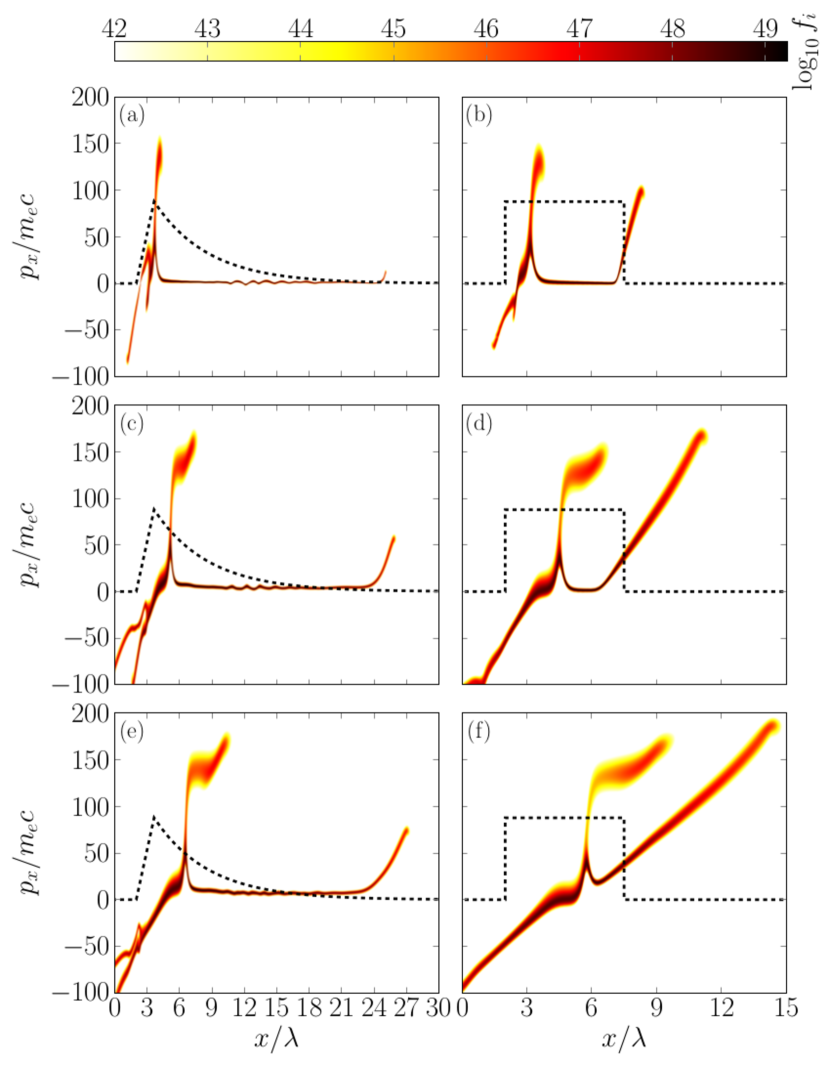
Figure 1: Ion phase-space distribution at three different time instants ( $t=39T$, $75T$ and $108T$) for the exponential (left) and rectangular (right) plasma density profiles. The target is irradiated by a linearly polarized pulse with $a_{0}=2.5$ and pulse length $50$ fs.

To investigate the effect of the density profile, we also consider a rectangular plasma slab with $n_{0}=2.5n_{c}$ and thickness $d=5.5\lambda$. The length of the slab was chosen so that the particle number is the same for both the rectangular and exponential density profiles. The ion distribution at three time instances ($t=39T$, $75T$ and $108T$) is shown in the right panels of Fig. 1. The dynamics of the shock-formation is similar for both cases, but the shock-velocity is slightly lower and closer to the hole-boring velocity. It is $0.037c$ in the rectangular case compared with $0.041c$ for the exponential case. Furthermore, the TNSA is stronger than in the exponential case, resulting in a TNSA-dominated broad ion energy spectrum, as can be seen in Fig. 2 (blue dashed line). From this we can conclude that the shape of the density profile at the rear side has an important role in suppressing the sheath-field responsible for TNSA. Similar conclusions were drawn in Refs. 13; 14, where electrostatic shocks driven by the interaction of two plasmas with different density and relative drift velocity were studied using PIC simulations.

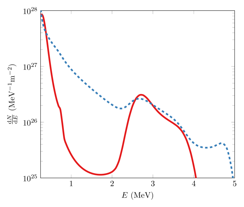
Figure 2: Proton spectrum at $t=108T$ for the exponentially decreasing density profile (red solid) and the rectangular plasma slab (blue dashed).

The energy spectrum given in Fig. 2 was calculated based on the entire ion population using $\text{d}N/\text{d}E=\left(\text{d}p/\text{d}E\right)\int f_{i}(x,p_{x})\,\text{d}x$, where $E=\sqrt{m^{2}c^{4}+p^{2}c^{2}}$ and $f_{i}(x,p_{x})$ is the ion distribution function. Note, that the exact value of the initial ion temperature does not influence the results, as long as the ions are cold at the start of the simulation. A simulation with the same laser-pulse and target parameters, but an initial ion temperature of $T_{i}=100\;\rm eV$ gives identical results. This also applies to a simulation with an initial electron temperature of $T_{e}=2.5\;\rm keV$.

Figure 3 shows the longitudinal electric field as a function of time and space for the exponential and rectangular density profiles. From Fig. 3a it can be noted that the sheath-field at the rear side of the exponential density profile is smaller than the one at the shock-front. This, combined with the fact that regions with significant electric fields at the rear side are associated with lower ion density, leads to less pronounced TNSA. Therefore the resulting ion spectrum has a broad bump-like structure with a maximum ion energy at around 3 MeV, as shown in Fig. 2 (red solid line); contrasted with the rectangular density profile, for which the proton spectrum is shown with a blue dashed line. In the latter case, the sheath-field at the rear side is very strong, as can be seen in Fig. 3b, and gives rise to the broad exponential proton spectrum that is typical for cases when TNSA is dominant.

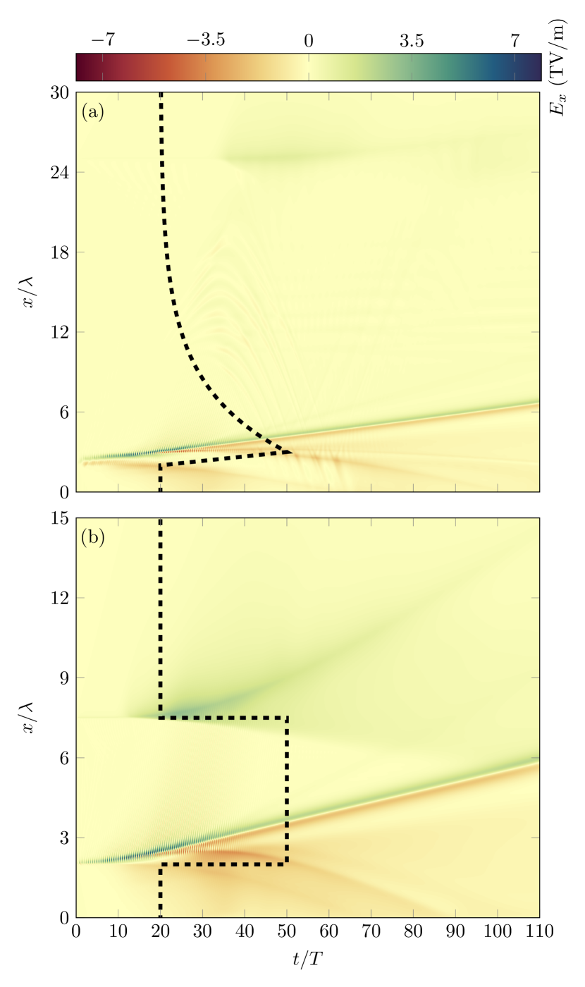
Figure 3: Longitudinal electric field as a function of position and time for the (a) exponential and (b) rectangular density profiles. The target is irradiated by a linearly polarized pulse with $a_{0}=2.5$ and pulse length $50$ fs.

III.2 Laser pulse variation

Pulse intensity

Here, we show results for the exponential density profile heated by a laser pulse with $a_{0}=2.5\sqrt{2}$ and pulse length $25\,\mathrm{fs}$. With these parameters the laser fluency is the same as in the case with the longer and less intense pulse described in the previous subsection. Figure 4 shows the ion distribution function at times $t=39T$, $75T$, $108T$ and $240T$. Compared to the case with the longer pulse with lower intensity (both the rectangular and exponential profiles), the time for the shock to develop is considerably longer. The velocity of the shock-wave in the more intense pulse case is also higher, with $v_{s}=0.049c$.

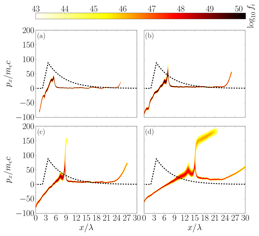
Figure 4: Ion phase-space distribution for the exponential density profile irradiated by a linearly polarized pulse with $a_{0}=2.5\sqrt{2}$ and pulse length 25 fs at $t=39T$, $75T$, $108T$ and $240T$.

At first it may seem counterintuitive that the shock is developed later in the case of the shorter and more intense pulse, given the fact that the shock-velocity is higher. The main reason for the later development is the shorter pulse length and higher intensity, which leads to operation close to the onset of relativistic transparency and larger peneteration of the pulse into the plasma rather than reflection/compression at the plasma vacuum interface. This gives smaller peak ion and electron densities after interaction with the laser pulse and results in differences in the electrostatic potential and the reflection time of the ions.

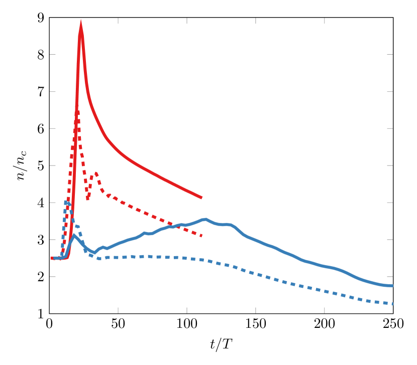
Figure 5: Peak ion (solid) and electron (dashed) densities as functions of time. Red lines: $a_{0}=2.5$. Blue lines: $a_{0}=2.5\sqrt{2}$.

In both cases the ion and electron densities have their largest peak value right after the interaction with the pulse. For the shorter pulse case however, the peak values are much lower (see Fig. 5). These lower ion and electron densities lead to a more gradual and wider potential barrier.

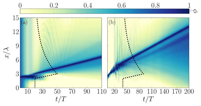
Figure 6: Electrostatic potential as function of space and time. (a) $a_{0}=2.5$ and pulse length 50 fs, (b) $a_{0}=2.5\sqrt{2}$ and pulse length 25 fs.

Figure 6 shows the electrostatic potential as a function of time and space for the exponential density profile in the cases with different laser intensities and pulse lengths ($a_{0}=2.5$ left panel, $a_{0}=2.5\sqrt{2}$ right panel). The potential is scaled and shifted according to $2e\phi/m_{p}v_{s}^{2}-\max{[2e\phi/m_{p}v_{s}^{2}]}+1$, such that the peak of the potential is unity. Furthermore, the potential has been truncated at zero. When the laser pulse hits the target there is an oscillation in the densities and electrostatic potential, due to $\mbox{\boldmath$j$}\times\mbox{\boldmath$B$}$-heating. The frequency of the oscillation is approximately twice the laser frequency. For the more intense pulse these oscillations persist for a longer time.

For ions at a low temperature, reflection occurs for a potential barrier height approximately equal to unity. If the ions have acquired a velocity in the direction of the shock, reflection occurs at a slightly smaller barrier height, which is the case at later times due to sheath-expansion of the target. Hence, a shock solution may develop although the potential barrier initially does not have sufficient height for ion reflection to occur.

For a linearly rising potential barrier, the reflection time for an ion is given by $d/v_{s}$, where $d$ is the spatial extent of the barrier. As mentioned before, the potential barrier for the shorter and more intense pulse is initially wider (see Fig. 6), yielding a proportionally longer reflection time. Even if the shock-velocity is slightly higher in the more intense case, the spatial extent of the barrier is even larger, so the reflection time, $d/v_{s}$, is longer.

Figure 5 shows a steepening of the peak ion density from $t\simeq 25T$ to $t\simeq 100T$ in the case of the shorter and more intense pulse (solid blue line). This steepening is associated with persisting oscillations in the electrostatic potential. The width of the potential barrier is reduced and therefore the reflection time for the ions as well. Finally, a shock is developed, albeit much later than in the case of the longer pulse. This shows that shock acceleration can be operated close to the relativistic transparency regime which maximizes the hole-boring velocity and is also seen to yield a higher shock velocity.

Pulse splitting

Previous numerical results indicate that using a train of short laser pulses may produce more efficient ion-acceleration than one Gaussian pulse with the same energy mironov ; yu ; markey . Furthermore, experimental results in Ref. 11 show that a smooth pulse containing the same energy as a pulse train will result in a monotonically decreasing ion spectrum, instead of a spectrum with a well-defined peak as in the pulse-train case. This indicates that the efficiency of shock-acceleration is improved in the case of multiple pulses.

To investigate how the splitting of the pulse affects the shock-dynamics, here we consider the exponential density profile irradiated by two laser pulses with $a_{0}=2.5$ and pulse length $25\,\mathrm{fs}$, that are separated by $50\,\mathrm{fs}$ in time. Figure 7 shows the electrostatic potential as a function of time and space. The variation in the electrostatic potential indicates that a shock-structure is formed already after the first pulse. The arrival of the second pulse perturbs the potential barrier associated with the shock, leading to a slight increase of its velocity, from $v_{s}\approx 0.030c$ to $v_{s}\approx 0.039c$. Hence, the use of two pulses increases the velocity of the shock, although it remains smaller than if all the energy would have been in a single pulse, c.f. $v_{s}\approx 0.041c$ for a single pulse with $a_{0}=2.5$ and pulse length 50 fs.

Figure 7: Electrostatic potential in the case of the exponential density profile irradiated by two laser pulses with $a_{0}=2.5$ and pulse lengths $25\,\mathrm{fs}$, that are separated by $50\,\mathrm{fs}$ in time.

The effect of pulse-splitting is even more important for higher initial plasma densities, as predicted by previous numerical and experimental results, see e.g. Ref. 27. The reason is that the absorption of the second pulse can be enhanced if the target density at the front side becomes lower due to heating-induced expansion caused by the first pulse. This results in higher electron temperatures and consequently stronger TNSA. This heating-induced absorption enhancement effect is not as pronounced if the initial densities are close to the critical density. Our simulations show that for a rectangular density profile with $n_{0}=25n_{c}$, the energy spectrum is TNSA-dominated and the cutoff ion energy is increased by 10% in the case of two pulses with $a_{0}=2.5$ and pulse lengths 25 fs separated in time with 50 fs, compared with the case of one pulse with $a_{0}=2.5$ and pulse length 50 fs. Corresponding simulations with peak densities $n_{0}<2.5n_{c}$ do not give a substantial increase in the proton energy if the pulse is split.

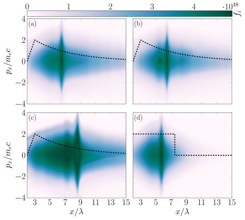
Figure 8: Electron phase-space distribution at $t=108T$ in the exponential and rectangular density profile cases. Panels (a) and (d) show the case with $a_{0}=2.5$ and pulse length $50\,\mathrm{fs}$, for the exponential (a) and rectangular (d) plasma profiles. Panel (b) depicts the exponential density profile irradiated by two laser pulses with $a_{0}=2.5$ and pulse length $25\,\mathrm{fs}$, that are separated by $50\,\mathrm{fs}$ in time. Panel (c) is for the exponential profile with $a_{0}=2.5\sqrt{2}$ and pulse length 25 fs.

Figure 8 shows snapshots at $t=108T$ of the electron distribution function for both the exponential and the rectangular profiles for different values of $a_{0}$ and pulse shapes. The simulations confirm that the hot electron temperature in all cases is on the order of magnitude of the ponderomotive scaling $T_{h}\approx m_{e}c^{2}(\sqrt{1+a_{0}^{2}/2}-1)$. Specifically, the case with the more intense pulse (with shortest pulse length), leads to the highest hot electron temperature, as expected from the ponderomotive scaling, even if the fluency is the same in the different cases. The Mach number of the shocks $M=v_{s}/c_{s}$ is around 1.7 in all cases, if we use the ponderomotive scaling to estimate the hot electron energy as the temperature in the sound speed $c_{s}=\sqrt{T_{e}/m_{i}}$.

IV Enhanced ion acceleration using multi-ion species layered targets

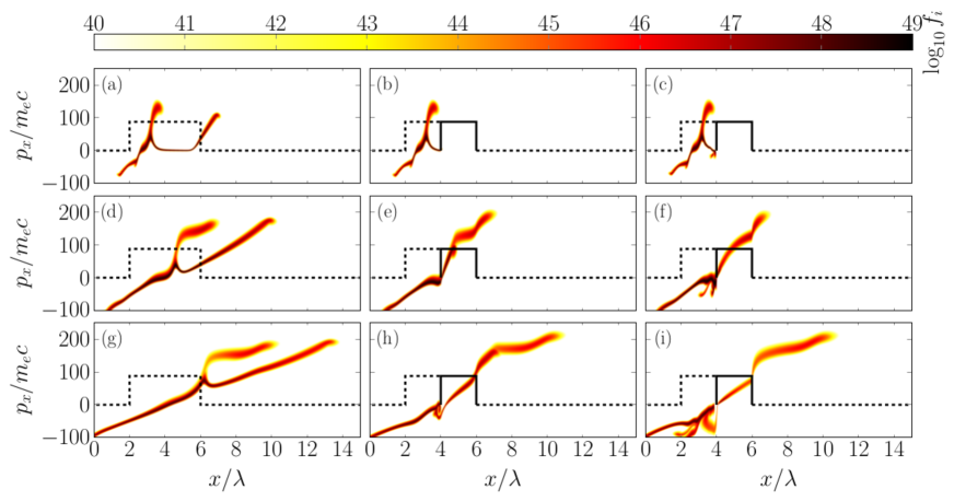
Figure 9: Ion phase-space distribution for single- and double-layer target structures, irradiated by a linearly polarized pulse with $a_{0}=2.5$ and pulse length 50 fs at $t=39T$, $75T$ and $108T$. (a,d,g) show the single-species target, (b,e,h) the layered target with $n=2.5n_{c}$ and (c,f,i) the layered target with the high density heavy ion layer having $n=25n_{c}$.

For a target with a steep rear boundary, a strong sheath-field can be obtained and used to increase the energy of shock-accelerated ions. Targets with a single light ion species are subject to significant TNSA and hence the resulting ion energy-spectrum becomes broad. Furthermore, the acceleration of ions at the rear side leads to a decay of the sheath-field strength and hence its usefulness for post-acceleration is reduced. To combine the use of a strong sheath-field for post-acceleration and a low degree of TNSA, we consider a double layered rectangular target consisting of a layer of light ions (protons) at the front side ($x\in[2\lambda,4\lambda]$) and heavy (immobile) ions at the rear side ($x\in[4\lambda,6\lambda]$). We use the density profile $n(x)=2.5n_{c}$ in the light ion part. In the heavy ion part we consider two cases for the electron density profile, $n(x)=2.5n_{c}$ and $n(x)=25n_{c}$, respectively. For comparison, we also consider a single layer rectangular target with protons $n(x)=n_{0}$ for $x\in[2\lambda,6\lambda]$. The targets are irradiated by a laser pulse with $a_{0}=2.5$ and pulse length $50\,\mathrm{fs}$.

Figure 9 shows snapshots of the ion distribution function for the single-species and double layered targets at $t=39T$, $75T$ and $108T$. The laser heats the front side of the target and launches a shock. Until the shock reaches the region with heavy ions in the double layer, its behaviour is similar to that in the single species target. For the double-layered targets the shock wave is stopped at the interface between the layers, but the shock-wave reflected ions continue and finally cross the rear side of the target. When this occurs the ions are further accelerated due to the sheath field, leading to higher proton energies than what they would have from the reflection by the shock-wave alone.

If the heavy ion layer has higher density than the light ion layer, ions can be slowed down due to the sheath field that is created by the density difference at the interface. Those ions that have acquired enough energy from the shock-wave potential barrier can penetrate the interface and continue through the target. The interface between the layers acts effectively as a filter: it reflects the low energy ions, and leads to a narrower energy spectrum after the interface. By comparing Figs. 9(h,i) we see that more protons penetrate the interface in the low density case, as can be expected since the size of the potential barrier associated with the sheath field at the interface between the light ion and heavy ion layers is smaller in this case.

Inside the heavy ion layer, the energy spectrum ranges from zero for protons that had initial energy just above the threshold for reflection, to the highest energy of reflected ions, reduced by the size of the potential barrier. The electric field inside the heavy ion layer is very small, so the protons are crossing this layer without gaining much energy. As it takes less time for the higher energy light ions to cross the heavy ion layer, the distribution is rotated in phase-space, as can be noted by comparing e.g. Figs. 9(f,i). When the light ions reach the interface to vacuum, they are accelerated by the strong sheath-field there.

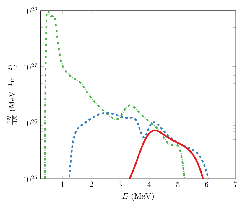
Figure 10: Proton spectrum at $t=108T$ for single-species and double-layered targets. Green dash-dotted line is for the single-species target. Blue dashed line is for the layered target with $n=2.5n_{c}$. Red solid line is for the layered target with the high density heavy ion layer having $n=25n_{c}$.

In all cases the maximum proton energies exceed the energy of 2.9 MeV for reflected ions by the shock-wave, as can be seen in Fig. 10, where the proton spectrums in the three cases are presented. Furthermore, in the single species case we have a broad TNSA-dominated proton spectrum. For the layered targets we observe that the range of the spectrum shrinks and the maximum proton energy increases compared to the single species case. The shrinkage of the spectrum is stronger in the high density case. In other words, by choosing the density of the heavy ion layer appropriately it should be possible to further optimize the monoenergeticity of the ion beam. As mentioned before, the reason is that the longitudinal electric field in the boundary region between the light and heavy ion part of the layered target is stronger in the high density case, which hinders the penetration of low energy ions to the high density region. However, those ions that cross that boundary and reach the rear side of the target will be efficiently accelerated.

The number of accelerated ions can be increased by using a thicker proton layer on the front side of a double-layer target. Then the shock will be sustained for a longer time, as in the single species case, where the shock is sustained throughout the whole target width. To quantify the increase in particle number, we can compare the number of shock-accelerated ions at different time instances in a simulation with a target that has larger spatial extent. For example, for the case with the exponential density profile and laser parameters $a_{0}=2.5\sqrt{2}$, pulse length 25 fs, the numbers of shock accelerated ions at $t=200T$ and $t=240T$ are 1.60 and 2.14 times larger than that at $t=160T$.

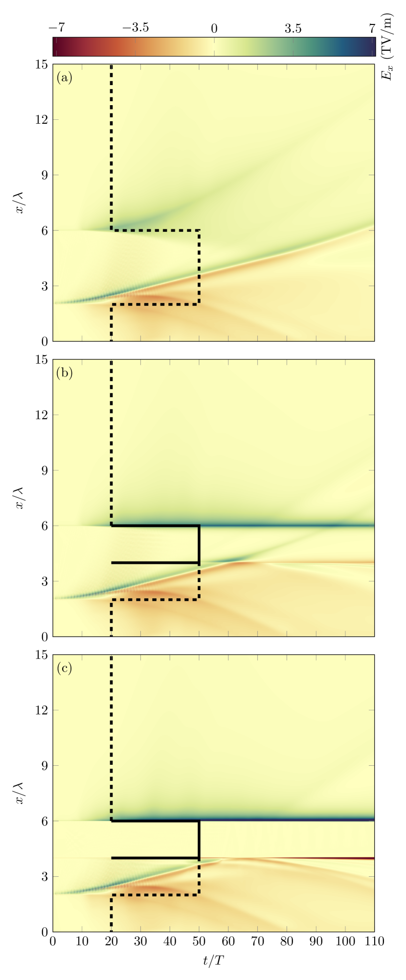
Figure 11: Longitudinal electric field as a function of position and time for targets irradiated by a linearly polarized pulse with $a_{0}=2.5$ and pulse length 50 fs. (a) shows the single-species target, (b) the layered target with $n=2.5n_{c}$ and (c) the layered target with the high density heavy ion layer having $n=25n_{c}$.

Figure  11 shows the electric field as a function of position and time in the layered targets compared with the single species one. During the initial part of the simulation, the sheath-field is set up by the hot electrons that are generated by the laser-pulse. For the single-species target, the sheath field changes its structure in time as the plasma expands at the rear boundary. On the other hand, for the double layered targets, the sheath field is stronger and has less time variation. The strongest sheath field is obtained in the high density case, with a maximum value of 10 TV/m. Note that in the Fig. 11 we only show values up to the maximum value for the low density case (7 TV/m). Our simulations show that as long as the $A/Z\gtrsim 10$ the temporal variation of the sheath field will not affect the quality of the shock-accelerated protons.

V Conclusions

Vlasov-modelling of collisionless shock-acceleration allows for high resolution of the distribution function, and therefore is highly suitable in cases where effects of low-density tails in the distribution function need to be resolved accurately. In this paper we have restricted the discussion to 1D1P modelling for simplicity. Although the shock-dynamics is expected to be slightly different in the 2D case, the main conclusions should be valid, given the fact that particle-in-cell simulations have shown only a few percent differences in the energy cutoff of the ions between 1D and 2D configurations silva ; lecz .

We show that by using a target with a smooth (e.g. exponentially decreasing) density profile at the rear side, TNSA can be kept at a low level, making CSA the main mechanism of acceleration of particles. On the other hand, the energy of the shock-wave accelerated ions could potentially be increased by the sheath-field produced at the rear side. Provided that the sheath-field has limited variation in time, mono-energeticity of the ions may be preserved. Early launch of the shock increases the number of ions that are reflected and can be optimized by an appropriate choice of laser-parameters and also potentially the density profile.

We observe that for the same laser fluency, a higher intensity combined with a shorter laser pulse duration leads to a higher shock-velocity, but the Mach-number is only slightly increased. The main difference compared to the lower intensity and longer pulse length case is that the shock develops later. This may be due that the shorter duration of the laser pulse leads to a less peaked ion-density and hence wider potential barrier, which results in a longer reflection time for the ions. We show that splitting the laser-pulse can also lead to higher shock-velocities, but without the delay of the shock-formation.

Our simulations show that by using a target which consists of light ions on the front side and heavy ions on the rear side, it is possible to combine a strong quasi-static sheath-field with CSA. The dynamics of shock-formation in the double-layer target resembles the one in a rectangular single-species plasma slab, but as soon as the light ions pass the rear side of the target, they obtain higher energies due to a strong sheath field, which is produced due to the charge-separation between the electrons that penetrate the rear side of the target and the heavy ions at rest. This leads to very efficient acceleration and an increase in the proton energies compared to the energies of shock-reflected ions, without broadening of the energy spectrum if the heavy ion layer has high density.

VI Appendix

VI.1 Numerical description of one dimensional conservation laws

Consider a conservation law:

$$\partial_{t}f+\partial_{\zeta}\left[a(\zeta,t)f\right]=0,$$ (10)

which may be either Eq. (7) or Eq. (8). Introduce the mapping $X(s,t,\zeta)$:

$$\left\{\begin{array}[]{l}\frac{\text{d}X(s,t,\zeta)}{\text{d}s}=a[X(s,t,\zeta),s]\\ X(t,t,\zeta)=\zeta\end{array}\right.$$ (11)

and a discretization $(\zeta_{i},t_{j})=(i\Delta\zeta,j\Delta t)$. It then holds that:

$$\int_{\zeta_{i-\frac{1}{2}}}^{\zeta_{i+\frac{1}{2}}}f(\zeta,t_{j+1})\,\text{d}\zeta=\int_{X(t_{j},t_{j+1},\zeta_{i-\frac{1}{2}})}^{X(t_{j},t_{j+1},\zeta_{i+\frac{1}{2}})}f(\zeta,t_{j})\,\text{d}\zeta,$$ (12)

which can be written as:

$$\begin{array}[]{r}\int_{\zeta_{i-\frac{1}{2}}}^{\zeta_{i+\frac{1}{2}}}f(\zeta,t_{j+1})\,\text{d}\zeta=\int_{\zeta_{i-\frac{1}{2}}}^{\zeta_{i+\frac{1}{2}}}f(\zeta,t_{j})\,\text{d}\zeta\\ -\int_{X(t_{j},t_{j+1},\zeta_{i+\frac{1}{2}})}^{\zeta_{i+\frac{1}{2}}}f(\zeta,t_{j})\,\text{d}\zeta\\ +\int_{X(t_{j},t_{j+1},\zeta_{i-\frac{1}{2}})}^{\zeta_{i-\frac{1}{2}}}f(\zeta,t_{j})\,\text{d}\zeta.\end{array}$$ (13)

Introducing cell-averaged discrete values of the distribution function:

$$f_{i}^{j}=\frac{1}{\Delta\zeta}\int_{\zeta_{i-\frac{1}{2}}}^{\zeta_{i+\frac{1}{2}}}f(\zeta,t_{j})\,\text{d}\zeta$$ (14)

and fluxes $\phi_{i+\frac{1}{2}}$:

$$\phi_{i+\frac{1}{2}}=\frac{1}{\Delta\zeta}\int_{X(t_{j},t_{j+1},\zeta_{i+\frac{1}{2}})}^{\zeta_{i+\frac{1}{2}}}f(\zeta,t_{j})\,\text{d}\zeta,$$ (15)

Eq. (13) can be written as:

$$f_{i}^{j+1}=f_{i}^{j}-\phi_{i+\frac{1}{2}}+\phi_{i-\frac{1}{2}}.$$ (16)

The choice of method to evaluate $X(t_{j},t_{j+1},\zeta_{i+\frac{1}{2}})$ and the corresponding flux $\phi_{i+\frac{1}{2}}$ determines the accuracy of the method.

For the non-relativistic Vlasov-Poisson equation, $a(\zeta,t)$ is independent of $\zeta$ and $X(t_{j},t_{j+1},\zeta_{i+\frac{1}{2}})$ can be determined to second order accuracy by:

$$X(t_{j},t_{j+1},\zeta_{i+\frac{1}{2}})=\zeta_{i+\frac{1}{2}}-a(t_{j+\frac{1}{2}})\Delta t.$$ (17)

For the relativistic Vlasov-Maxwell system on the other hand, $a(\zeta,t)$ is not independent of $\zeta$ and Eq. (17) yields a first order accurate approximation of $X(t_{j},t_{j+1},\zeta_{i+\frac{1}{2}})$.

To evaluate the fluxes $\phi_{i+\frac{1}{2}}$, we use the positive and flux conservative method filbet . The distribution function $f(\zeta)$, in the cell with index $i$, is approximated in terms of the cell averaged values with indices $(i-1)$, $i$ and $(i+1)$, according to:

$$f(\zeta) =f_{i}+\frac{\epsilon_{i}^{+}}{6\Delta\zeta^{2}}[2(\zeta-\zeta_{i})(\zeta-\zeta_{i-\frac{3}{2}})$$

$$+(\zeta-\zeta_{i-\frac{1}{2}})(\zeta-\zeta_{i+\frac{1}{2}})](f_{i+1}-f_{i})$$

$$+\frac{\epsilon_{i}^{-}}{6\Delta\zeta^{2}}[2(\zeta-\zeta_{i})(\zeta-\zeta_{i+\frac{3}{2}})$$

$$+(\zeta-\zeta_{i-\frac{1}{2}})(\zeta-\zeta_{i+\frac{1}{2}})](f_{i}-f_{i-1}),$$

where we have suppressed the time-index $j$. Furthermore, the limiters $\epsilon^{+}_{i}$ and $\epsilon^{-}_{i}$ are given by:

$$\epsilon^{+}_{i}=\left\{\begin{array}[]{lr}\min\left(1,\frac{2f_{i}}{f_{i+1}-f_{i}}\right)&\text{ if }f_{i+1}>f_{i}\\ \min\left(1,-2\frac{f_{\infty}-f_{i}}{f_{i+1}-f_{i}}\right)&\text{ if }f_{i}>f_{i+1}\end{array}\right.$$ (18)

and:

$$\epsilon^{-}_{i}=\left\{\begin{array}[]{lr}\min\left(1,2\frac{f_{\infty}-f_{i}}{f_{i}-f_{i-1}}\right)&\text{ if }f_{i}>f_{i-1}\\ \min\left(1,\frac{-2f_{i}}{f_{i}-f_{i-1}}\right)&\text{ if }f_{i-1}>f_{i}\end{array}\right..$$ (19)

The quantity $f_{\infty}$ is the maximum cell-averaged value. Straightforward integration yields the flux:

$$\begin{array}[]{r}\phi_{i+\frac{1}{2}}=\alpha[f_{i}+\frac{\epsilon^{+}_{i}}{6}(1-\alpha)(2-\alpha)(f_{i+1}-f_{i})\\ +\frac{\epsilon_{i}^{-}}{6}(1-\alpha)(1+\alpha)(f_{i}-f_{i-1})]\end{array}$$ (20)

if $a_{i+\frac{1}{2}}$ is positive, where $\alpha=[\zeta_{i+\frac{1}{2}}-X(t_{j},t_{j+1},\zeta_{i+\frac{1}{2}})]/\Delta\zeta$. For negative $a_{i+\frac{1}{2}}$, we instead have:

$$\begin{array}[]{r}\phi_{i+\frac{1}{2}}=\alpha[f_{i+1}-\frac{\epsilon^{+}_{i+1}}{6}(1-\alpha)(1+\alpha)(f_{i+2}-f_{i+1})\\ -\frac{\epsilon_{i+1}^{-}}{6}(2+\alpha)(1+\alpha)(f_{i+1}-f_{i})].\end{array}$$ (21)

This is a third order interpolation of the fluxes, except in the presence of steep gradients. The limiters ensure that the interpolation is positivity preserving and does not violate the maximum principle. Finally, as boundary conditions, we set the fluxes across boundaries to zero which enforces that particles can not leave or enter the domain and yields strict particle conservation.

VI.2 Discretization of the electromagnetic field equations

By introducing the quantities:

$$G_{\pm}=E_{z}\pm cB_{y}\quad\text{and}\quad F_{\pm}=E_{y}\pm cB_{z},$$

we may write:

$$\left(\frac{\partial}{\partial t}\pm c\frac{\partial}{\partial x}\right)F_{\pm}=-J_{y}/\epsilon_{0}$$ (22)

$$\left(\frac{\partial}{\partial t}\pm c\frac{\partial}{\partial x}\right)G_{\mp}=-J_{z}/\epsilon_{0}.$$ (23)

Introducing characteristics $\eta=t+x/c$ and $\nu=t-x/c$, it holds that:

$$\left(\frac{\partial}{\partial t}+c\frac{\partial}{\partial x}\right)F_{+}=2\frac{\partial F_{+}}{\partial\eta}$$

$$\left(\frac{\partial}{\partial t}-c\frac{\partial}{\partial x}\right)F_{-}=2\frac{\partial F_{-}}{\partial\nu}$$ (24)

as well as:

$$\left(\frac{\partial}{\partial t}+c\frac{\partial}{\partial x}\right)G_{-}=2\frac{\partial G_{-}}{\partial\eta}$$

$$\left(\frac{\partial}{\partial t}-c\frac{\partial}{\partial x}\right)G_{+}=2\frac{\partial G_{+}}{\partial\nu}.$$ (25)

To advance the equations (22) and (23), we take $c\Delta t=|\Delta x|$ and use a second order accurate central difference scheme:

$$F^{j+\frac{1}{2}}_{\pm,(i+\frac{1}{2}\pm 1)}=F_{\pm,(i+\frac{1}{2})}^{j-\frac{1}{2}}-\Delta tJ^{j}_{y,(i+\frac{1}{2}\pm\frac{1}{2})}/\epsilon_{0},$$ (26)

$$G^{j+\frac{1}{2}}_{\pm,(i+\frac{1}{2}\mp 1)}=G_{\pm,(i+\frac{1}{2})}^{j-\frac{1}{2}}-\Delta tJ^{j}_{z,(i+\frac{1}{2}\mp\frac{1}{2})}/\epsilon_{0}$$ (27)

where $i$ is an index for the spatial-coordinate and $j$ is an index for the temporal-coordinate.

Additionally, the electric field component $E_{x}$ is calculated by:

$$E_{x,(i+\frac{1}{2})}^{j+\frac{1}{2}}=\rho_{i}^{j+\frac{1}{2}}\Delta x+E_{x,(i-\frac{1}{2})}^{j+\frac{1}{2}},$$ (28)

which is second order accurate, provided that the charge density can be determined with first order accuracy.

Regarding boundary conditions, the laser pulse is implemented as a Dirichlet boundary condition for the transverse fields and we use open boundary conditions at the boundary that is not associated with the laser. For the electric field component $E_{x}$ we have the Dirichlet boundary condition $E_{x}=0$ at the right boundary.

Finally, defining the discretized vector-potential on the spatial cell-faces, it can be calculated with second order accuracy in time on integer time-steps by using a central-difference approximation of the time-derivative in $\partial\mbox{\boldmath$A$}_{\perp}/\partial t=-\mbox{\boldmath$E$}_{\perp}$.

References

- (1) H. Daido, M. Nishiuchi, and A. S. Pirozhkov, Rev. Prog. Phys 75, 056401 (2012).
- (2) A. Macchi, M. Borgesi, and M. Passoni, Rev. Mod. Phys. 85, 751 (2013).
- (3) I. Spencer, K. W. D. Ledingham, R. P. Singhal, T. McCanny, P. McKenna, E. L. Clark, K. Krushelnick, M. Zepf, F. N. Beg, M. Tatarakis, A. E. Dangor, P. A. Norreys, R. J. Clarke, R. M. Allott, I. N. Ross, Nucl. Inst. Methods in Phys. Reserarch 183, 449 (2001).
- (4) R. Orecchia, A. Zurlo, A. Loasses, M. Krengli, G. Tosi, S. Zurrida, P. Zucali, U. Veronesi, Eur. J. Cancer, 34, 459 (1998).
- (5) U. Amaldi, Nucl. Phys. A, 654, C375 (1999).
- (6) S. V. Bulanov, T. Z. Esirkepov, V. S. Khoroshkov, A. V. Kuznetsov, and F. Pegoraro, Phys. Lett. A 299, 240 (2002).
- (7) V. Malka, S. Fritzler, E. Lefebvre, E. d’Humiéres, R. Ferrand, G. Grillon, C. Albaret, S. Meyroneinc, J.-P. Chambaret, A. Antonetti, and D. Hulin, Med. Phys. 31, 1587 (2004).
- (8) M. Borghesi, D. H. Campbell, A. Schiavi, M. G. Haines, O. Willi, A. J. MacKinnon, P. Patel, L. A. Gizzi, M. Galimberti, R. J. Clarke, F. Pegoraro, H. Ruhl, and S. Bulanov, Phys. Plasmas 9, 2214 (2002).
- (9) S. C. Wilks. A. B. Langdon, T. E. Cowan, M. Roth, M. Singh, S. Hatchett, M. H. Key, D. Pennington, A. MacKinnon, and R. A. Snavely, Phys. Plasmas 8, 542 (2001).
- (10) L. Silva, M. Marti, J. R. Davies, R. A. Fonseca, Phys. Rev. Lett. 92, (2004).
- (11) D. Haberberger, S. Tochitsky, F. Fiuza, C. Gong, R. A. Fonseca, L. O. Silva, W. B. Mori, and C. Joshi, Nat. Phys. 8, 95 (2012).
- (12) A. Macchi, A. Singh Nindrayog and F. Pegoraro, Phys. rev. E 85, 046402 (2012).
- (13) F. Fiuza, A. Stockem, E. Boella, R. A. Fonseca, L. O. Silva, D. Haberberger, S. Tochitsky, W. B. Mori, and C. Joshi, Phys. Plasmas 20, 056304 (2013).
- (14) F. Fiuza, A. Stockem, E. Boella, R. A. Fonseca, L. O. Silva, D. Haberberger, S. Tochitsky, C. Gong, W. B. Mori, and C. Joshi, Phys. Rev. Lett. 109, 215001 (2012).
- (15) F. Huot, A. Ghizzo, P. Bertrand, E. Sonnendrücker, O. Coulaud, J. Comp. Phys. 185, 512 (2003).
- (16) C. Z. Cheng et al, J. Comp. Phys. 22, 330 (1976).
- (17) N. J. Sircombe, T. D. Arber, J. Comp. Phys. 228, 4773 (2009).
- (18) A. Ghizzo, F. Huot, P. Bertrand, J. Comp. Phys. 186, 47 (2003).
- (19) T. D. Arber, R. G. L. Vann, J. Comp. Phys. 180, 339 (2002).
- (20) F. Filbet, E. Sonnendrücker, and P. Bertrand, J. Comp. Phys. 172, 166 (2001).
- (21) E. Sonnendrücker, J. Roche, P. Bertrand, and A. Ghizzo, J. Comp. Phys. 149, 201 (1999).
- (22) S. Bastrakov, R. Donchenko, A. Gonoskov, E. Efimenko, A. Malyshev, I. Meyerov, I. Surmin, J. Comp. Science 3, 474 (2012).
- (23) A. Grassi, L. Fedeli, A. Sgattoni, A. Macchi, submitted to Plasma Phys. Control. Fusion, arXiv:1507.08585.
- (24) A. V. Korzhimanov, A. A. Gonoskov, A. V. Kim, A. M. Sergeev, JETP 105, 675 (2007).
- (25) V. Mironov, N. Zharova, E. d’Humiéres, R. Capdessus, and V. T. Tikonchuk, Plasma Phys. Control. Fusion, 54 095008, (2012).
- (26) W. Yu, L.Cao, M. Y. Yu, H. Cai, H. Xu, X. Yang, A. Lei, K. A. Tanaka, and R. Kodama, Laser Part. Beams 27, 109 (2009).
- (27) K. Markey, P. McKenna, C. M. Brenner, D. C. Carroll, M. M. Günther, K. Harres, S. Kar, K. Lancaster, F. Nürnberg, M. N. Quinn, A. P. L. Robinson, M. Roth, M. Zepf, and D. Neely, Phys. Rev. Lett. 105, 195008 (2010)
- (28) Zs. Lécz and A. Andreev, Phys. Plasmas 22, 043103 (2015).