Banded operational matrices for Bernstein polynomials and application to the fractional advection-dispersion equation

Abstract

In the papers dealing with derivation and applications of operational matrices of Bernstein polynomials, a basis transformation, commonly a transformation to power basis, is used. The main disadvantage of this method is that the transformation may be ill-conditioned. Moreover, when applied to the numerical simulation of a functional differential equation, it leads to dense operational matrices and so a dense coefficient matrix is obtained. In this paper, we present a new property for Bernstein polynomials. Using this property, we build exact banded operational matrices for derivatives of Bernstein polynomials. Next, as an application, we propose a new numerical method based on a Petrov-Galerkin variational formulation and the new operational matrices utilizing the dual Bernstein basis for the time-fractional advection-dispersion equation. We show that the proposed method leads to a narrow-banded linear system and so less computational effort is required to obtain the desired accuracy for the approximate solution. We also obtain the error estimation for the method. Some numerical examples are provided to demonstrate the efficiency of the method and to support the theoretical claims.

1 Introduction

Bernstein polynomials play an important role in computer aided geometric design (farin2002, ). Moreover, these polynomials provide a tool in the numerical simulation of differential, integral and integro-differential equations; see e.g., (malek2012, ; maleknejad2011, ; Youzbasi, ) and the references therein. In recent decades, many authors discovered some new analytic properties and also some applications for these polynomials. For example, Cheng (cheng1983, ) derived the rate of convergence of these polynomials for a certain class of functions. Farouki (farouki2-1996, ) showed that among nonnegative bases on a given interval, the Bernstein polynomials basis is an optimal stable basis. Delgado et al. (delgado2009, ) proved that the collocation matrices of the Bernstein basis are the best conditioned among all the collocation matrices of nonnegative totally positive bases on a given interval.

On the other hand, a basis transformation, commonly to the power basis $\{1,x,\dots,x^{N}\}$, is used in order to derive the operational matrices for the derivatives and integrals of Bernstein polynomials. The developed numerical method for differential and integral equations based on those matrices leads to a linear system whose coefficient matrix is neither banded nor sparse; see, for instance, (malek2012, ; pandey, ; parand, ; saadatmandi2014, ; Yousefi2010, ; Yousefi2011, ). It is also worth to note that the explicit conversion between the Bernstein basis and the power basis is exponentially ill-conditioned (Farouki1999, ).

In this paper, we directly derive narrow-banded operational matrices for the derivatives of Bernstein polynomials without using any basis transformation and we show that it leads to less computational cost and less round-off errors. Then, as an application, we propose a numerical scheme for the time fractional advection-dispersion equation (FAD). In the proposed method, we use the Bernstein polynomials as the trial functions and the dual Bernstein polynomials as the test functions for the Petrov-Galerkin variational formulation. We then show that under some reasonable assumptions, the derived linear system has a unique solution.

Due to various applications of fractional advection-dispersion equation in the mathematical modeling of some important physical problems, many classical numerical methods for the partial differential equations have been developed to handle this problem. For example, Gao et al. (Gao, ) proposed a numerical scheme based on a compact finite difference method. Shirzadi et al. (Shirzadi, ) implemented the meshless methods. Jiang et al. (Jiang, ) developed a finite element method. Stokes et al. (Stok, ) used a mapping from the associated Brownian counterpart for the numerical solution of the time-fractional advection-dispersion equation.

This paper is concerned with providing a new numerical method for the time-fractional advection-dispersion equation given by

$${D_{t}^{\alpha}}u\left(x,t\right)=\kappa_{1}\frac{\partial^{2}}{\partial x^{2}}u\left(x,t\right)-\kappa_{2}\frac{\partial}{\partial x}u\left(x,t\right)+S(x,t),\quad\left(x,t\right)\in\Omega\times\left(0,\infty\right),$$ (1.1)

where $u$ is the unknown concentration, $\kappa_{1}$ and $\kappa_{2}$ are the dispersion and advection coefficients, $\alpha\in\left(0,1\right)$ is the temporal fractional order, $S$ is the known source term, the operator $D_{t}^{\alpha}$ represents the Caputo fractional derivative and $\Omega=\left(0,L\right).$

Definition 1

(Diethelm, ) The Caputo fractional derivative of order $\alpha>0$ is defined by

$${D^{\alpha}}f(x)=\frac{1}{\Gamma(m-\alpha)}\int_{0}^{x}{\frac{1}{(x-s)^{\alpha-m+1}}\frac{d^{m}f(s)}{ds^{m}}ds},\quad x>0,$$

where $m:=\left\lceil\alpha\right\rceil$.

So the Caputo temporal fractional derivative of order $\alpha$ is written as

$${D_{t}^{\alpha}}u(x,t)=\frac{1}{\Gamma(m-\alpha)}\int_{0}^{t}{\frac{1}{(t-s)^{\alpha-m+1}}\frac{\partial^{m}u(x,s)}{\partial s^{m}}ds}.$$ (1.2)

We consider the equation (1.1) with the following initial and boundary conditions

$$u\left(x,0\right)=g\left(x\right),\quad x\in\left[0,L\right],$$ (1.3)

$$u\left(0,t\right)=0,\quad u\left(L,t\right)=0,\quad t>0.$$ (1.4)

This paper is organized as follows. In Section 2, we introduce some background material of Bernstein polynomials. Section 3 is devoted to some new relations for Bernstein basis and the derivation of new banded operational matrices. In Section 4, we use the new operational matrices and the Petrov-Galerkin variational formulation to develop a numerical simulation for the time-fractional advection-dispersion equation. The error analysis for the method is discussed in Section 5. Some numerical examples are carried out in Section 5. The paper ends with some concluding remarks in Section 7.

2 Preliminaries

We first provide the definition and some preliminary results for Bernstein polynomials.

The Bernstein polynomials of degree $N\geq 0$ on $[a,b]$ are defined by

$$B_{i,N}(x)=\frac{\dbinom{N}{i}(x-a)^{i}(b-x)^{N-i}}{(b-a)^{N}},\qquad 0\leq i\leq N.$$ (2.1)

We adopt the convention $B_{i,N}(x)\equiv 0$ for $i<0$ and $i>N$. The set $B_{N}=\left\{B_{i,N}(x):\,i=0,\dots,N\right\}$ is a basis for $\mathbb{P}_{N}$, the space of polynomials of degree not exceeding $N$.

The base functions satisfy the endpoint interpolation property, i.e.

$$B_{i,N}(a)=\delta_{i,0},\quad B_{i,N}(b)=\delta_{i,N},\quad 0\leq i\leq N,\,N\geq 0.$$ (2.2)

It is useful in the numerical formulation of the problem when imposing boundary conditions. Also, for $N\geq 1,$ the basis has the following degree elevation property:

$$B_{i,N-1}(x)=\frac{1}{N}\left[\left(N-i\right)B_{i,N}(x)+\left(i+1\right)B_{i+1,N}(x)\right],\quad 0\leq i\leq N.$$

This relation may be recursively used to get the following general formula.

Lemma 1

[farouki1988, , Relation (26)] Let $i,\,j$ and $N$ be nonnegative integers, $j\leq N$ and $i\leq N-j$. Then,

$$B_{i,N-j}(x)=\binom{N-j}{i}\sum_{r=i}^{j+i}\frac{\binom{j}{r-i}}{\binom{N}{r}}B_{r,N}(x).$$ (2.3)

The derivatives of the Bernstein polynomials satisfy the following recurrence relation [farouki1988, , Relation (54)]

$$B_{i,N}^{\prime}(x)=\frac{N}{b-a}\left(B_{i-1,N-1}(x)-B_{i,N-1}(x)\right),\quad 0\leq i\leq N.$$

Using the Leibniz’s rule, we derive the following result (see [doha2-2011, , Theorem 3.1.] for a similar result on the unit interval).

Lemma 2

Let $N$ and $p$ be nonnegative integers and $p\leq N$. Then, for $0\leq i\leq N,$

$$B_{i,N}^{(p)}(x)=c_{p,N}\sum_{k=\max{(0,i+p-N)}}^{\min{(i,p)}}(-1)^{k}\dbinom{p}{k}B_{i-k,N-p}(x),$$ (2.4)

where

$$c_{p,N}=\frac{\left(-1\right)^{p}N!}{(b-a)^{p}(N-p)!}.$$ (2.5)

Theorem 2.1

[juttler, , Theorem 3.] The elements of the dual basis $B_{N}^{\star}=\left\{B_{i,N}^{\star}(x):\,i=0,\dots,N\right\}$ associated with the Bernstein basis $B_{N}$ on $[a,b]$ are given by

$$B_{i,N}^{\star}(x)=\sum_{j=0}^{N}d_{i,j}B_{j,N}(x),\quad 0\leq i\leq N,$$ (2.6)

with the coefficients

$$d_{i,j}=\frac{(-1)^{i+j}}{(b-a)\binom{N}{i}\binom{N}{j}}\sum_{r=0}^{min(i,j)}(2r+1)\binom{N+r+1}{N-i}\binom{N-r}{N-i}\binom{N+r+1}{N-j}\binom{N-r}{N-j},$$

for $i,j=0,1,\dotsc,N$. Two sets $B_{N}$ and $B_{N}^{\star}$ form a biorthogonal system, i.e.

$$\int_{a}^{b}B_{i,N}(x)B_{j,N}^{\star}(x)dx=\delta_{ij},$$ (2.7)

for $i,j=0,1,\dots,N$.

3 Banded operational matrices for derivatives of Bernstein polynomials

The existing operational matrices for Bernstein basis and the applications are based on a basis transformation, commonly from Bernstein to power basis (see, for instance,(malek2012, ; pandey, ; parand, ; saadatmandi2014, ; Yousefi2010, ; Yousefi2011, )). The transformation may be ill-conditioned, and also it does not lead to banded linear systems (Farouki1999, ). In this section, we first obtain a new representation for derivatives of Bernstein polynomials and then present banded operational matrices.

The representation (2.4) for $p$th order derivative of Bernstein polynomials changes the basis order from $N$ to $N-p$. For the Galerkin and Petrov-Galerkin formulations of the equation (1.1), we need to express the derivatives in terms of the same basis functions. So we state the following theorem.

Theorem 3.1

Let $N$ be any nonnegative integer and $0\leq i\leq N$. Then, for any nonnegative integer $p\leq N,$ we have the following “at most $(2p+1)$ term” relation

$$B_{i,N}^{(p)}(x)=c_{p,N}\sum_{j=\max(0,i-p)}^{\min(N,i+p)}\omega_{i,j}B_{j,N}(x),\quad 0\leq i\leq N,$$ (3.1)

where $c_{p,N}$ is defined as (2.5) and the coefficients are as follows:

$$\omega_{i,j}=\sum_{k=\max(0,i-j)}^{\min(p,i-j+p)}{\mu_{i,k,j}},$$

$$\mu_{i,k,j}=(-1)^{k}\frac{\binom{p}{k}\binom{N-p}{i-k}\binom{p}{j-i+k}}{\binom{N}{j}}.$$ (3.2)

Proof

By using (2.3) and (2.4), we obtain the following relation

$$B_{i,N}^{(p)}(x) = c_{p,N}\sum_{k=\max{(0,i+p-N)}}^{\min{(i,p)}}{(-1)^{k}\binom{p}{k}\binom{N-p}{i-k}\sum_{j=i-k}^{i-k+p}{\frac{\binom{p}{j-i+k}}{\binom{N}{j}}B_{j,N}(x)}}$$

$$= c_{p,N}\sum_{k=m}^{n}{\left(\sum_{j=i-k}^{i-k+p}{\mu_{i,k,j}B_{j,N}(x)}\right)},$$

where $m=\max{(0,i+p-N)}$ and $n=\min{(i,p)}$. The summation limits are $m\leq k\leq n$ and $i-k\leq j\leq i-k+p$, changing the order of summation as $i-n\leq j\leq i-m+p$ and $i-j\leq k\leq i-j+p$ and noting that $i+p-m=\min{(N,i+p)}$ and $i-n=\max{(0,i-p)},$ we get

$$B_{i,N}^{(p)}(x) = c_{p,N}\sum_{j=\max{(0,i-p)}}^{\min{(N,i+p)}}{\left(\sum_{k=i-j}^{i-j+p}{\mu_{i,k,j}}\right)B_{j,N}(x)}.$$

Due to the fact that $\mu_{i,k,j}=0$ for $k<0$ and $k>p$, by removing the zero terms, we obtain:

$$B_{i,N}^{(p)}(x) = c_{p,N}\sum_{j=\max{(0,i-p)}}^{\min{(N,i+p)}}{\left(\sum_{k=\max(0,i-j)}^{\min(p,i-j+p)}{\mu_{i,k,j}}\right)B_{j,N}(x)}$$

$$= c_{p,N}\sum_{j=\max(0,i-p)}^{\min(N,i+p)}\omega_{i,j}B_{j,N}(x).$$

This ends the proof. ∎

Remark 1

For $p=1$ and $p=2$, the relation (3.1) is written as

$$B_{i,N}^{\prime}(x)=\frac{1}{b-a}((N-i+1)B_{i-1,N}(x)-(N-2i)B_{i,N}(x)-(i+1)B_{i+1,N}(x)),$$ (3.3)

$$B_{i,N}^{\prime\prime}(x)=\frac{1}{\left(b-a\right)^{2}}((N-i+2)(N-i+1)B_{i-2,N}(x)-2(N-i+1)(N-2i+1)B_{i-1,N}(x)\,$$ (3.4)

$$\qquad+(N^{2}-6Ni+6i^{2}-N)B_{i,N}(x)+2(i+1)(N-2i-1)B_{i+1,N}(x)+(i+2)(i+1)B_{i+2,N}(x)),$$

for $i=0,1,\dots,N$.

Let $\phi=[B_{i,N}(x):\,i=0,1,...,N]^{T}$. By using (3.1), we have

$$\frac{d^{p}}{dx^{p}}\phi = \mathbf{D}_{p}\phi,\quad p\geq 1,$$

where $\mathbf{D}_{p}$ is a $(2p+1)$-diagonal, or $(p,p)$-banded, matrix expressed as

$$\mathbf{D}_{p}=c_{p,N}\left[\begin{array}[]{ccccccccccc}\omega_{0,0}&&\cdots&&\omega_{0,p}\\ \omega_{1,0}&&&\cdots&&\omega_{1,p+1}\\ \vdots\\ \omega_{p,0}&&&&&&\omega_{p,2p}\\ &\omega_{p+1,1}&&&&\cdots&&\omega_{p+1,2p+1}\\ &&\omega_{p+2,2}&&&&\cdots&&\omega_{p+2,2p+2}\\ &&&\ddots&&&&&\ddots\\ \\ \\ \\ &&&&&&&&\omega_{N,N-p}&\cdots&\omega_{N,N}\end{array}\right].$$

The above matrix, written according to Theorem 3.1, avoids matrix multiplications $\mathbf{D}_{p}=\mathbf{D}_{1}^{p}$.

Remark 2

We especially note that $\mathbf{D}_{0}=\mathbf{I}$, the identity matrix, $\mathbf{D}_{1}$ is the following tridiagonal matrix:

$$\mathbf{D}_{1}=\frac{1}{b-a}\left[\begin{array}[]{cccccc}-N&-1&0&&\cdots&0\\ N&2-N&-2&0&&\vdots\\ 0&N-1&4-N&-3&0\\ &0&\ddots&\ddots&\ddots&0\\ \vdots&&0&2&N-2&-N\\ 0&\cdots&&0&1&N\end{array}\right],$$

and $\mathbf{D}_{2}$ is a pentadiagonal matrix with elements given by

$$\left(\mathbf{D}_{2}\right)_{i,j} = \frac{1}{\left(b-a\right)^{2}}\times\begin{cases}\begin{array}[]{cc}(N-i+2)(N-i+1),&i-j=-2,\\ -2(N-i+1)(N-2i+1),&i-j=-1,\\ N^{2}-6Ni+6i^{2}-N,&i-j=0,\\ 2(i+1)(N-2i-1),&i-j=1,\\ (i+2)(i+1),&i-j=2,\\ 0,&\left|i-j\right|>2.\end{array}&i,j=0,\ldots.,N.\end{cases}$$

Remark 3

For $\mathbf{D}_{1}$, it is seen that sum of the elements in each column is zero. This holds for $\mathbf{D}_{p}$, $p\geq 1$. To see this, let $0\leq j\leq N$ and $p>1$. Then,

$$\sum_{i=0}^{N}{(\mathbf{D}_{p})_{i,j}} = \sum_{i=0}^{N}{(\mathbf{D}_{1}\mathbf{D}_{p-1})_{i,j}}=\sum_{i=0}^{N}{\sum_{k=0}^{N}{(\mathbf{D}_{1})_{i,k}(\mathbf{D}_{p-1})_{k,j}}}$$

$$= \sum_{k=0}^{N}{(\mathbf{D}_{p-1})_{k,j}\sum_{i=0}^{N}{(\mathbf{D}_{1})_{i,k}}}=0.$$

Here we present some other interesting features of $\mathbf{D}_{p}$.

Lemma 3

Let $p$ be a positive integer. Then $\mathbf{D}_{p}$ is a nilpotent matrix, i.e., $\mathbf{D}_{p}^{k}=0$ for some positive integer $k$. In fact the smallest such $k$ is $k=\left\lceil\frac{N+1}{p}\right\rceil$ where $\left\lceil\cdot\right\rceil$ represents the ceiling function, i.e., the smallest following integer.

Proof

Let $i\leq j$. Then,

$$(\mathbf{D}_{1}^{N})_{i,j} = (\mathbf{D}_{N})_{i,j}=c_{N,N}\sum_{k=\max(0,i-j)}^{\min(N,i-j+N)}{\mu_{i,k,j}}$$

$$= c_{N,N}\sum_{k=0}^{N+i-j}{(-1)^{k}\frac{\binom{N}{k}\binom{0}{i-k}\binom{N}{j-i+k}}{\binom{N}{j}}}$$

$$= c_{N,N}(-1)^{i}\binom{N}{i}.$$

Similarly, for $i>j$ we obtain $(\mathbf{D}_{1}^{N})_{i,j}=c_{N,N}(-1)^{i}\binom{N}{i}$, and so

$$(\mathbf{D}_{1}^{N})_{i,j} = c_{N,N}(-1)^{i}\binom{N}{i},\quad 0\leq i,j\leq N.$$ (3.5)

This means that for each row of $\mathbf{D}_{1}^{N}$, all the entries are the same, and we obtain

$$(\mathbf{D}_{1}^{N+1})_{i,j} = \sum_{k=0}^{N}{(\mathbf{D}_{1}^{N})_{i,k}(\mathbf{D}_{1})_{k,j}}$$

$$= c_{N,N}(-1)^{i}\binom{N}{i}\sum_{k=0}^{N}{(\mathbf{D}_{1})_{k,j}},$$

for $0\leq i,j\leq N+1$. From Remark 3, the last summation is zero and so $\mathbf{D}_{1}^{N+1}=0$. It means that $\mathbf{D}_{1}$ is nilpotent. Since $\mathbf{D}_{1}^{N}\neq 0$ by (3.5), $\mathbf{D}_{1}$ is a nilpotent matrix with index $N+1$. Let $k=\left\lceil\frac{N+1}{p}\right\rceil$. Using $kp\geq N+1$ and the fact that $\mathbf{D}_{p}=\mathbf{D}_{1}^{p}$, we obtain

$$\mathbf{D}_{p}^{k} = \mathbf{D}_{1}^{kp}=0.$$

On the other hand, since $(k-1)p<N+1$ so $\mathbf{D}_{p}^{k-1}=\mathbf{D}_{1}^{(k-1)p}\neq 0$ and so $\mathbf{D}_{p}$ is a nilpotent matrix with index $k$. This completes the proof. ∎

The following corollary is obtained from the fact that $\mathbf{D}_{p}$ is nilpotent (see (Serre, ), for more properties of nilpotent matrices).

Corollary 1

Let $p\geq 1$ and $0\leq i,j\leq N$, then

(a) All the eigenvalues of $\mathbf{D}_{p}$ are zero,

(b) $trace(\mathbf{D}_{p})=0,$

(c) $\mathbf{I}-c\mathbf{D}_{p}$ is nonsingular for any scalar $c\in\mathbb{C}$ and

$$(\mathbf{I}-c\mathbf{D}_{p})^{-1} = \mathbf{I}-c\mathbf{D}_{1}^{p}+c^{2}\mathbf{D}_{1}^{2p}-c^{3}\mathbf{D}_{1}^{3p}+\cdots+(-1)^{k}c^{k}\mathbf{D}_{1}^{kp}$$

with the largest integer $k$ that $kp\leq N$.

The following result, makes some savings in storage especially for much larger matrices.

Proposition 1

Let $p\geq 1$ and $0\leq i,j\leq N$, then

$$(\mathbf{D}_{p})_{i,j}=(-1)^{p}(\mathbf{D}_{p})_{N-i,N-j},\,i,j\geq 0.$$

Proof

For the nonzero elements of $\mathbf{D}_{p}$, from (3.1), we have

$$(\mathbf{D}_{p})_{N-i,N-j} = c_{p,N}\omega_{N-i,N-j}=c_{p,N}\sum_{k=\max(0,j-i)}^{\min(p,j-i+p)}{(-1)^{k}\frac{\binom{p}{k}\binom{N-p}{N-i-k}\binom{p}{(N-j)-(N-i)+k}}{\binom{N}{N-j}}}.$$

To make the manipulations easier, we remove the max and min on the summation limits (the only difference is that some zeros are added), so

$$(\mathbf{D}_{p})_{N-i,N-j} = c_{p,N}\sum_{k=j-i}^{j-i+p}{(-1)^{k}\frac{\binom{p}{k}\binom{N-p}{N-i-k}\binom{p}{i-j+k}}{\binom{N}{j}}}$$

$$= c_{p,N}\sum_{k=i-j}^{i-j+p}{(-1)^{k}\frac{\binom{p}{k-2i+2j}\binom{N-p}{N-k+i-2j}\binom{p}{k-i+j)}}{\binom{N}{j}}}.$$

Reversing the order of the last summation using $\sum_{k=m}^{n}a_{k}$=$\sum_{k=m}^{n}a_{m+n-k}$, we get

$$(\mathbf{D}_{p})_{N-i,N-j} = c_{p,N}\sum_{k=i-j}^{i-j+p}{(-1)^{2i-2j+p-k}\frac{\binom{p}{p-k}\binom{N-p}{N-i-p+k}\binom{p}{i-j+p-k}}{\binom{N}{j}}}$$

$$= c_{p,N}\sum_{k=i-j}^{i-j+p}{(-1)^{p-k}\frac{\binom{p}{k}\binom{N-p}{i-k}\binom{p}{j-i+k}}{\binom{N}{j}}}$$

$$= (-1)^{p}c_{p,N}\sum_{k=\max(0,i-j)}^{\min(p,i-j+p)}{(-1)^{k}\frac{\binom{p}{k}\binom{N-p}{i-k}\binom{p}{j-i+k}}{\binom{N}{j}}}$$

$$= (-1)^{p}c_{p,N}\sum_{k=\max(0,i-j)}^{\min(p,i-j+p)}{\mu_{i,k,j}}$$

$$= (-1)^{p}c_{p,N}\omega_{i,j}=(-1)^{p}(\mathbf{D}_{p})_{i,j}.$$

This completes the proof. ∎

Remark 4

Corresponding to the non-orthogonal Bernstein basis, the associated orthonormalized basis $\{Q_{i,N}(x):\,i=0,\dots,N\}$ is obtained by using the Gram-Schmidt algorithm. This basis fails to have properties like (3.3) and (3.4). To see this, let $i=4$ and $N=4$. Then, it can be verified that

$$Q_{i,N}^{\prime}(x)=\sum_{i=0}^{N}c_{i}Q_{i,N}(x),$$

in which all the coefficients $c_{0},\dots,c_{4}$ are nonzero. It is also worth noting that the Chebyshev and Legendre polynomials do not have properties like (3.3) and (3.4). In fact, the differentiation matrix of Chebyshev and also Legendre polynomial basis of degree $N$ have ${\it[\frac{N}{2}]}$ nonzero diagonals (see (SaadatLegendre, ) and [Shen, ,Sections 3.3 and 3.4] for more details).

4 A new numerical method for the time-fractional advection-dispersion equation

This section is devoted to providing a numerical method using the new Bernstein polynomial operational matrices with the Petrov-Galerkin method for the problem (1.1) subject to the initial condition given by (1.3) and the homogeneous boundary conditions (1.4).

We rewrite the advection-dispersion equation (1.1) at $t=t_{k+1},\,k\geq 0$ as

$${D_{t}^{\alpha}}u(x,t_{k+1})=\kappa_{1}\frac{\partial^{2}}{\partial x^{2}}u(x,t_{k+1})-\kappa_{2}\frac{\partial}{\partial x}u(x,t_{k+1})+S(x,t_{k+1}),\quad x\in\Omega.$$

Without loss of generality, we consider the problem (1.1)-(1.4) on the bounded domain $\Omega_{T}=[0,1]\times[0,T]$. Let $t_{k}=k\tau$, $k=0,1,\dots,M$ where $\tau=\frac{T}{M}$ is the time step length. Then, the time fractional derivative at time $t_{k+1}$ is approximated as

$${D_{t}^{\alpha}}u(x,t_{k+1})=\frac{1}{\Gamma(1-\alpha)}\sum_{j=0}^{k}\frac{u(x,t_{j+1})-u(x,t_{j})}{\tau}\int_{t_{j}}^{t_{j+1}}\frac{ds}{(t_{k+1}-s)^{\alpha}}+r_{\tau}^{k+1},\quad k\geq 0,$$

with the error term $r_{\tau}^{k+1}$. Consequently,

$${D_{t}^{\alpha}}u(x,t_{k+1})=\mu_{\tau}^{\alpha}\sum_{j=0}^{k}a_{k,j}^{\alpha}\left(u\left(x,t_{j+1}\right)-u\left(x,t_{j}\right)\right)+r_{\tau}^{k+1},$$ (4.1)

where $\mu_{\tau}^{\alpha}=\frac{1}{\tau^{\alpha}\Gamma(2-\alpha)}$ and $a_{kj}^{\alpha}=\left(k+1-j\right)^{1-\alpha}-\left(k-j\right)^{1-\alpha}$ for $k\geq 0$ and $j=0,1,\dots,k$. A bound for the error is given by

$$|r_{\tau}^{k+1}| \leq \tilde{c}_{u}\tau^{2-\alpha},$$ (4.2)

where the coefficient $\tilde{c}_{u}$ depends only on $u$ (Deng, ). The scheme described here for time discretization is known as $L_{1}$ approximation, a common way in the numerical simulation of partial fractional differential equations, for instance, see, (Deng, ; Gao, ; Rame, ). Similar to (Deng, ; Gao, ), we define the time discrete fractional differential operator $L_{t}^{\alpha}$ as

$$L_{t}^{\alpha}u(x,t_{k+1})=\mu_{\tau}^{\alpha}\sum_{j=0}^{k}a_{k,j}^{\alpha}\left(u^{j+1}\left(x\right)-u^{j}\left(x\right)\right),$$ (4.3)

in which $u^{j}(x)$ is an approximation for $u(x,t_{j})$. So from (4.1), we have

$${D_{t}^{\alpha}}u(x,t_{k+1})=L_{t}^{\alpha}u(x,t_{k+1})+r_{\tau}^{k+1}.$$

Using $L_{t}^{\alpha}u(x,t_{k+1})$ as an approximation for ${D_{t}^{\alpha}}u(x,t_{k+1})$ in (1.1) yields the following time-discrete scheme:

$$\mu_{\tau}^{\alpha}\sum_{j=0}^{k}a_{k,j}^{\alpha}\left(u^{j+1}\left(x\right)-u^{j}\left(x\right)\right)=\kappa_{1}\frac{\partial^{2}u^{k+1}(x)}{\partial x^{2}}-\kappa_{2}\frac{\partial u^{k+1}(x)}{\partial x}+S^{k+1}(x),$$ (4.4)

for $k=0,...,M-1,$ from which we have

$$\boldsymbol{L}u^{k+1}:=\mu_{\tau}^{\alpha}u^{k+1}(x)-\kappa_{1}\frac{\partial^{2}u^{k+1}(x)}{\partial x^{2}}+\kappa_{2}\frac{\partial u^{k+1}(x)}{\partial x}=f^{k+1}(x),$$ (4.5)

where $f^{k+1}(x)=\mu_{\tau}^{\alpha}\left(u^{k}(x)-\sum_{j=0}^{k-1}a_{k,j}^{\alpha}\left(u^{j+1}\left(x\right)-u^{j}\left(x\right)\right)\right)+S^{k+1}(x)$. Note that $u^{0}(x)=g(x)$ is given by the initial condition (1.3) and the $f^{k+1}(x)$ is a known function at time step $t_{k+1}$. For the error analysis , it will be useful to consider the homogeneous case $S=0$, multiply the semidiscrete problem (4.5) by $\tau^{\alpha}\Gamma(2-\alpha)$, rearrange the involving summation and dropping $x$, to get (Lin, ; Rame, )

$$u^{k+1}-\alpha_{1}\frac{\partial^{2}u^{k+1}}{\partial x^{2}}+\alpha_{2}\frac{\partial u^{k+1}}{\partial x}=(1-b_{1})u^{k}+\sum_{j=1}^{k-1}(b_{j}-b_{j+1})u^{k-j}+b_{k}u^{0},\quad k\geq 1,$$ (4.6)

and for $k=0$

$$u^{1}-\alpha_{1}\frac{\partial^{2}u^{1}}{\partial x^{2}}+\alpha_{2}\frac{\partial u^{1}}{\partial x}=u^{0},$$ (4.7)

where $\alpha_{i}=\kappa_{i}\tau^{\alpha}\Gamma(2-\alpha),\,i=1,2$ and

$$b_{j} = (j+1)^{1-\alpha}-j^{1-\alpha},\quad j=0,1,\dots,k.$$ (4.8)

The boundary conditions are $u^{k+1}(0)=u^{k+1}(1)=0$ and the initial condition is $u^{0}=g(x)$. By (4.2), the error for (4.6), $r^{k+1}=\tau^{\alpha}\Gamma(2-\alpha)r_{\tau}^{k+1}$ is bounded as

$$|r^{k+1}|\leq c_{u}\tau^{2}.$$ (4.9)

To enforce the boundary conditions on the approximate solution, we set $\mathbb{P}_{N}^{0}=\{\phi\in\mathbb{P}_{n}:\,\phi(0)=\phi(1)=0\}$ with $dim(\mathbb{P}_{N}^{0})=N-1$. Define $\tilde{\Phi}=[\phi_{i}(x)=B_{i,N}(x):\,i=1,\dots,N-1]^{T},$ where from now on, we set $a=0$ and $b=1$. Since $\tilde{\Phi}$ is a basis for $X_{N}$, we can expand the approximate solution at time step $t=t_{k+1}$ as

$$u^{k+1}(x)\approx u_{N}^{k+1}(x)=\sum_{i=1}^{N-1}{c_{i}^{k+1}B_{i,N}(x)}=(\boldsymbol{c}^{k+1})^{T}\tilde{\phi},\quad k\geq 0,$$ (4.10)

where $\boldsymbol{c}^{k+1}=[c_{i}^{k+1}:\,i=1,\dots,N-1]^{T}$. It is easy to see that the associated differentiation matrices are given as

$$\tilde{\Phi}^{\prime}=\tilde{\mathbf{D}}_{1}\tilde{\Phi}+\boldsymbol{d}_{1},$$ (4.11)

$$\tilde{\Phi}^{\prime\prime}=\tilde{\mathbf{D}}_{2}\tilde{\Phi}+\boldsymbol{d}_{2},$$ (4.12)

where the tridiagonal and pentadiagonal matrices $\tilde{\mathbf{D}}_{1}$ and $\tilde{\mathbf{D}}_{2}$ are extracted respectively by removing the first and last rows and the first and last columns of $\mathbf{D}_{1}$ and $\mathbf{D}_{2}$. The $(N-1)$-dimensional vectors $\boldsymbol{d}_{1}$ and $\boldsymbol{d}_{2}$ are given by $\boldsymbol{d}_{1}=N[\phi_{0},0,\ldots.,0,-\phi_{N}]^{T}$ and $\boldsymbol{d}_{2}=N(N-1)[-2\phi_{0},\phi_{0},0,\ldots.,0,\phi_{N}-2\phi_{N}]^{T}$. By substituting (4.10) for $u^{k+1}$ in (4.5) and using (4.11) and (4.12), we get

$$\boldsymbol{L}u_{N}^{k+1}(x)=(\boldsymbol{c}^{k+1})^{T}(\mu_{\tau}^{\alpha}\tilde{\Phi}-\kappa_{1}(\tilde{\mathbf{D}}_{2}\tilde{\Phi}+\boldsymbol{d}_{2})+\kappa_{2}(\tilde{\mathbf{D}}_{1}\tilde{\Phi}+\boldsymbol{d}_{1})),$$

and the residual is given by

$$\boldsymbol{R}_{N}^{k+1}(x):=\boldsymbol{L}u_{N}^{k+1}(x)-f^{k+1}(x).$$

To obtain the expansion coefficients $\boldsymbol{c}_{k+1}$, we enforce the residual to be orthogonal to the dual basis functions $\psi_{j}:=B_{j,N}^{\star},\,j=1,\dots,N-1$ given by (2.6), i.e.,

$$((\boldsymbol{c}^{k+1})^{T}(\mu_{\tau}^{\alpha}\tilde{\Phi}-\kappa_{1}(\tilde{\mathbf{D}}_{2}\tilde{\Phi}+\boldsymbol{d}_{2})+\kappa_{2}(\tilde{\mathbf{D}}_{1}\tilde{\Phi}+\boldsymbol{d}_{1}))-f^{k+1},\,\psi_{j})=0,\quad j=1,\dots,N-1,$$ (4.13)

where $(\cdot,\cdot)$ is the standard $L^{2}-$inner product. Define the dual basis vector $\tilde{\Psi}^{T}=[\psi_{i}(x):\,i=1,\dots,N-1]$. Using the biorthogonal identity (2.7), we have $\tilde{\Phi}\Psi^{T}=\mathbf{I}_{N-1},$ the identity matrix of order $N-1$. Since $(\boldsymbol{d}_{1},\psi_{j})=0$ and $(\boldsymbol{d}_{2},\psi_{j})=0$ for $0<j<N,$ the above linear system can be written as a pentadiagonal linear system as follows:

$$\mathbf{A}\boldsymbol{c}^{k+1}=\boldsymbol{b}^{k+1},\quad k=0,1,\dots,M-1,$$ (4.14)

where

$$\mathbf{A}^{T}=\mu_{\tau}^{\alpha}\mathbf{I}_{N-1}-\kappa_{1}\tilde{\mathbf{D}}_{2}+\kappa_{2}\tilde{\mathbf{D}}_{1},$$ (4.15)

and $\boldsymbol{b}^{k+1}=[(f^{k+1},\psi_{i}):\,i=1,\dots,N-1]^{T}$. The integrals in $\boldsymbol{b}^{k+1}$ may be computed by a numerical method like Gauss quadrature rules. In our computational test examples, we use 20 point Gauss-Legendre rule on the unit interval.

It is worth to note that the coefficient matrix of the linear system (4.14) is independent of the time step $k$. So for a fixed $N$ and $M$, its $LU$-decomposition is performed just once and is used for all time steps. The LU-decomposition for a banded matrix with $2p+1$-bandwidth is done just by $O(Np^{2}$) arithmetic operations and the number of operations to modify the right hand side and performing back substitution is $O(Np)$ [Golub, , Section 4.3]. So obtaining the numerical solution of the problem (1.1) on the bounded domain $[0,1]\times[0,T]$ with the proposed method requires just $O(MNp(p+1))$ arithmetic operations.

Starting from $u_{N}^{0}=g(x)$, the approximate solution (4.10) at $t_{k+1},\,k\geq 0$ is obtained by solving the linear system (4.14).

The following result states the condition required for the existence of the solution for the linear system (4.14).

Lemma 4

Let $\left\|\cdot\right\|$ be an induced matrix norm and suppose that the time step length $\tau$ is such that

$$\kappa_{1}\|\tilde{\mathbf{D}}_{2}\|+\kappa_{2}\|\tilde{\mathbf{D}}_{1}\|<\mu_{\tau}^{\alpha}.$$ (4.16)

Then, the coefficient matrix $\mathbf{A}$ is nonsingular, i.e., the linear system (4.14) has a unique solution.

Proof

Assume that (4.16) holds and $\mathbf{A}$ is singular. Then, there is a nonzero vector $x$ with $\|x\|=1$ such that $\mathbf{A}^{T}x=0$ and so $\mu_{\tau}^{\alpha}=\|(\kappa_{1}\tilde{\mathbf{D}}_{2}-\kappa_{2}\tilde{\mathbf{D}}_{1})x\|.$ Then, $\mu_{\tau}^{\alpha}\leq\kappa_{1}\|\tilde{\mathbf{D}}_{2}\|+\kappa_{2}\|\tilde{\mathbf{D}}_{1}\|$ which contradicts (4.16). ∎

Note that $\mu_{\tau}^{\alpha}\rightarrow\infty$ as time mesh size tends to zero. So the principal significance of the lemma is that it allows one to choose time mesh size $\tau$ small enough in order to satisfy the condition (4.16). However, by Maple, we found that $\det\mathbf{A}\neq 0$ for $1\leq N\leq 100$ without imposing condition (4.16) on the parameters, except for advection and dispersion coefficients $\kappa_{1}>0$ and $\kappa_{2}>0$ which are positive due to the nature of the problem, and it can be written as

$$\det{\mathbf{A}}=\sum_{i=0}^{N-1}{\sum_{j=0}^{[\frac{N-i-1}{2}]}{d_{i,j}\kappa_{2}^{2j}}\kappa_{1}^{i}}>0,$$

with all positive coefficients $d_{i,j}$.

It is easy to verify that $\|\tilde{\mathbf{D}}_{1}\|_{\infty}=2(N-1)$ for $N\geq 4$ and

$$\|\tilde{\mathbf{D}}_{2}\|_{\infty}=\begin{cases}\begin{array}[]{cc}2N^{2}+10N-68,&7\leq N\leq 15,\\ 4N^{2}-28N+40,&N\geq 16.\end{array}\end{cases}$$

and therefore, from (4.15), we have

$$\|\mathbf{A\|_{\infty}}\leq\begin{cases}\begin{array}[]{cc}\mu+\kappa_{1}(2N^{2}+10N-68)+2\kappa_{2}(N-1),&7\leq N\leq 15,\\ \mu+\kappa_{1}(4N^{2}-28N+40)+2\kappa_{2}(N-1),&N\geq 16,\end{array}\end{cases}$$

but since we do not have a compact formula for $\|\mathbf{A}^{-1}\|_{\infty}$, we only provide the condition number of the coefficient matrix $\mathbf{A}$ for some numeric values.

In Table 1, we provide the condition number of $\mathbf{A}$ and compare it with the condition number of the Hilbert matrix $\mathbf{H}$, with respect to the infinity norm, i.e., $C_{\infty}(\mathbf{A}):=Cond_{\infty}(\mathbf{A})=\|\mathbf{A}\|_{\infty}\|\mathbf{A}^{-1}\|_{\infty}$ for $\alpha=0.5,\,\tau=1/40$ for numeric values of $\kappa_{1}$ and $\kappa_{2}$. It shows that the condition number of $\mathbf{A}$ is relatively small and the ratio $R_{\infty}=C_{\infty}(\mathbf{A})/C_{\infty}(\mathbf{H})\rightarrow 0$ as $N\rightarrow\infty$ where $N$ is the size of the matrix. So we can expect good numerical results. This is supported by the numerical examples in the next section. On the other hand, as we mentioned before the transformation between Bernstein and Power basis is ill-conditioned and should be avoided for large $N$. In (Farouki1999, ), Farouki showed that the transformation matrix has condition number $C_{\infty}\approx 3^{N+1}\sqrt{(N+1)/4\pi}$.

Table 1: Condition number of $\mathbf{A}$ and comparison with the condition number of the Hilbert matrix

	$N$	4	5	6	7	8	9	10	11
$\begin{array}[]{c}\kappa_{1}=0.1,\\ \kappa_{2}=2\end{array}$	$C_{\infty}(\mathbf{A})$	5.31	8.03	12.90	27.41	54.77	100.74	210.08	463.47
	$R_{\infty}$	1.87E-04	8.51E-06	4.44E-07	2.78E-08	1.62E-09	9.16E-11	5.94E-12	3.76E-13
$\begin{array}[]{c}\kappa_{1}=1,\\ \kappa_{2}=1\end{array}$	$C_{\infty}(\mathbf{A})$	1.57	1.73	1.86	7.33	11.76	19.78	34.82	63.57
	$R_{\infty}$	5.54E-05	1.84E-06	6.43E-08	7.45E-09	3.47E-10	1.80E-11	9.85E-13	5.15E-14

5 Error estimation

5.1 Stability and convergence of the semidiscrete scheme

We will carry out the error estimation for the homogeneous case of (1.1), i.e., for $S=0$.

Due to the presence of the first-order advection term, it is convenient for the error analysis to multiply both sides of (4.6) by an integrating factor and use a weighted variational formulation (see e.g., [Shen, ; Section 4.4]). However, in order to utilize the biorthogonality (2.7) providing banded sparse linear systems the matrix, the formulation of our method in Section 4 and the numerical computations in Section 6) are presented with the spectral formulation without weight function.

Multiplying (4.6) by $w=\exp(-\frac{\alpha_{2}}{\alpha_{1}}x)=\exp(-\frac{\kappa_{2}}{\kappa_{1}}x)$, the equation (4.6) is written as

$$wu^{k+1}-\alpha_{1}\frac{\partial}{\partial x}\left(w\frac{\partial u^{k+1}}{\partial x}\right)=w(1-b_{1})u^{k}+\sum_{j=1}^{k-1}(b_{j}-b_{j+1})wu^{k-j}+b_{k}wu^{0}.$$ (5.1)

The variational formulation is then written as

$$(u^{k+1},v)_{w}+\alpha_{1}(\frac{\partial u^{k+1}}{\partial x},\frac{\partial v}{\partial x})_{w}=(1-b_{1})(u^{k},v)_{w}$$

$$\quad\quad\quad+\sum_{j=1}^{k-1}(b_{j}-b_{j+1})(u^{k-j},v)_{w}+b_{k}(u^{0},v)_{w},\quad k\geq 1,\,\forall v\in H_{0,w}^{1}(\Omega),$$ (5.2)

and for $k=0,$

$$(u^{1},v)_{w}+\alpha_{1}(\frac{\partial u^{1}}{\partial x},\frac{\partial v}{\partial x})_{w}=(u^{0},v)_{w},\quad\forall v\in H_{0,w}^{1}(\Omega).$$ (5.3)

Accordingly the Galerkin spectral discretization is to find $u_{N}^{k+1}\in\mathbb{P}_{N}^{0}(\Omega)=H_{0,w}^{1}(\Omega)\cap\mathbb{P}_{N}(\Omega)$ such that

$$(u_{N}^{k+1},v_{N})_{w}+\alpha_{1}(\frac{\partial u_{N}^{k+1}}{\partial x},\frac{\partial v_{N}}{\partial x})_{w}=(1-b_{1})(u_{N}^{k},v_{N})_{w}$$

$$\quad\quad\quad+\sum_{j=1}^{k-1}(b_{j}-b_{j+1})(u_{N}^{k-j},v_{N})_{w}+b_{k}(u_{N}^{0},v_{N})_{w},\quad k\geq 1,\,\forall v_{N}\in\mathbb{P}_{N}^{0}(\Omega).$$ (5.4)

for $k=0,$

$$(u_{N}^{1},v_{N})_{w}+\alpha_{1}(\frac{\partial u_{N}^{1}}{\partial x},\frac{\partial v_{N}}{\partial x})_{w}=(u_{N}^{0},v_{N})_{w},\quad\forall v_{N}\in H_{0,w}^{1}(\Omega).$$ (5.5)

We define the following inner product and the associated energy norm on $H_{0,w}^{1}(\Omega)$:

$$(u,v)_{w}=\int_{\Omega}uvwd\Omega,\quad(u,v)_{1,w}=(u,v)_{w}+\alpha_{1}(\frac{\partial u}{\partial x},\frac{\partial v}{\partial x})_{w},\quad\|u\|_{1,w}=(u,u)_{1,w}^{\frac{1}{2}}.$$ (5.6)

It is worth noting that from $\kappa_{2}\leq\kappa_{1}$ as it happens for real advection diffusion problems, we get $0\leq w(x)\leq 1$ for $x\in\Omega$, so $L^{2}(\Omega)\subseteq L_{w}^{2}(\Omega)$ and $H^{1}(\Omega)\subseteq H_{w}^{1}(\Omega)$.

The following result presents the unconditional stability of the the scheme (5.2).

Theorem 5.1

The weak semidiscrete scheme (5.2) is unconditionally stable:

$$\|u^{k}\|_{1,w}\leq\|u^{0}\|_{w},\quad k=1,\dots,M.$$ (5.7)

Proof

Let $v=u^{1}$ in (5.3). Then,

$$(u^{1},u^{1})_{w}+\alpha_{1}(\frac{\partial u^{1}}{\partial x},\frac{\partial u^{1}}{\partial x})_{w}=(u^{0},u^{1})_{w}.$$

Using the Schwarz inequality, the inequality $\|v\|_{w}\leq\|v\|_{1,w}$, and dividing both sides by $\|u^{1}\|{}_{1,w}$, one immediately gets (5.7) for $k=1$. Now suppose that (5.7) holds for $k\leq n.$ Taking $v=u^{n+1}$ in (5.2), we get

$$(u^{n+1},u^{n+1})_{w}+\alpha_{1}(\frac{\partial u^{n+1}}{\partial x},\frac{\partial u^{n+1}}{\partial x})_{w}=(1-b_{1})(u^{n},u^{n+1})_{w}$$

$$\quad\quad\quad\hfill+\sum_{j=1}^{n-1}(b_{j}-b_{j+1})(u^{n-j},u^{n+1})_{w}+b_{n}(u^{0},u^{n+1})_{w}.$$

Note that the sequence $\{b_{j}\}$ defined in (4.8) is decreasing and converging to zero with $b_{0}=1$. Hence the RHS coefficients in equation (4.6) are positive. Again using $\|v\|_{w}\leq\|v\|_{1,w}$, the Schwarz inequality and dividing both sides by $\|u^{n+1}\|_{1,w}$, we get

$$\|u^{n+1}\|_{1,w} \leq (1-b_{1})\|u^{n}\|_{w}+\sum_{j=1}^{n-1}(b_{j}-b_{j+1})\|u^{n-j}\|_{w}+b_{n}\|u^{0}\|_{w}$$

$$\leq \left((1-b_{1})+\sum_{j=1}^{n-1}(b_{j}-b_{j+1})+b_{n}\right)\|u^{0}\|_{w}=\|u^{0}\|_{w},$$

that is (5.7) for $k=n+1$. This completes the proof. ∎

Theorem 5.2

Let $u(x,t)$ be the exact solution of the problem (1.1) with the initial and boundary conditions (1.3)-(1.4) and $u^{k},\,k=1,\dots,M,$ be the solution of the the semidiscrete problem (4.6). Then,

$$\|u(t_{k})-u^{k}\|_{1,w}\leq\frac{c_{u}}{1-\alpha}T^{\alpha}\tau^{2-\alpha},\quad 0<\alpha<1,$$ (5.8)

$$\|u(t_{k})-u^{k}\|_{1,w}\leq c_{u}T\tau,\quad\qquad\quad\,as\,\alpha\rightarrow 1.$$ (5.9)

Proof

We first prove that

$$\|u(t_{k})-u^{k}\|_{1,w}\leq\frac{c_{u}}{b_{k-1}}\tau^{2},\quad k=1,\dots,M.$$ (5.10)

Define $e^{k}:=u(t_{k})-u^{k}.$ By (1.1) and (4.7), we derive

$$(e^{1},v)_{w}+\alpha_{1}(\frac{\partial e^{1}}{\partial x},\frac{\partial v}{\partial x})_{w}=(e^{0},v)_{w}+(r^{1},v)_{w},\quad\forall v\in H_{0,w}^{1}(\Omega).$$

Let $v=e^{1}$, then using $e^{0}=0$, $\|v\|_{w}\leq\|v\|_{1,w}$ and (4.9), we obtain

$$\|e^{1}\|_{1,w}\leq c_{u}\tau^{2},$$ (5.11)

that is (5.10) for $k=1$. Now suppose that (5.10) holds for $k=1,\dots,n$. Using (1.1) and (4.6), we get

$$(e^{n+1},v)_{w}+\alpha_{1}(\frac{\partial e^{n+1}}{\partial x},\frac{\partial v}{\partial x})_{w}=(1-b_{1})(e^{n},v)_{w}$$

$$\quad\quad\quad+\sum_{j=1}^{n-1}(b_{j}-b_{j+1})(e^{n-j},v)_{w}+b_{n}(e^{0},v)_{w}+(r^{n+1},v)_{w},\quad\forall v\in H_{0,w}^{1}(\Omega).$$

Taking $v=e^{n+1}$, we have

$$\|e^{n+1}\|_{1,w}^{2} \leq (1-b_{1})\|e^{n}\|_{w}\|e^{n+1}\|_{1,w}+\sum_{j=1}^{n-1}(b_{j}-b_{j+1})\|e^{n-j}\|_{w}\|e^{n+1}\|_{1,w}+\|r^{n+1}\|_{w}\|e^{n+1}\|_{1,w},$$

$$\Rightarrow\|e^{n+1}\|_{1,w} \leq (1-b_{1})\frac{c_{u}}{b_{n-1}}\tau^{2}+\sum_{j=1}^{n-1}(b_{j}-b_{j+1})\frac{c_{u}}{b_{n-j-1}}\tau^{2}+c_{u}\tau^{2}$$

$$\leq \left((1-b_{1})+\sum_{j=1}^{n-1}(b_{j}-b_{j+1})+b_{n}\right)\frac{c_{u}}{b_{n}}\tau^{2}=\frac{c_{u}}{b_{n}}\tau^{2},$$

i.e., (5.10) holds for $k=n+1$. This proves the (5.10).

Applying the mean value theorem to the function $f(t)=t^{1-\alpha}$, $\exists\xi$ $k-1<\xi<k\leq M$ such that

$$b_{k-1}\tau^{-\alpha}=\frac{(k\tau)^{1-\alpha}-(\tau(k-1))^{1-\alpha}}{\tau}=(1-\alpha)(\xi\tau)^{-\alpha}\geq(1-\alpha)(k\tau)^{-\alpha}\geq(1-\alpha)(T)^{-\alpha},$$

so we obtain

$$\frac{c_{u}}{b_{k-1}}\tau^{2}\leq\frac{c_{u}}{1-\alpha}T^{\alpha}\tau^{2-\alpha}.$$ (5.12)

This together with (5.10) gives (5.8).

To prove (5.9), we first prove

$$\|u(t_{k})-u^{k}\|_{1,w}\leq c_{u}k\tau^{2},\quad k=1,\dots,M.$$ (5.13)

From (5.11), the relation (5.13) holds for $k=1$. Let (5.13) holds for $k=1,\dots,n,\>n\leq M-1$. Then, from (1.1), (4.6) and (4.9), we obtain

$$\|e^{n+1}\|_{1,w} \leq (1-b_{1})\|e^{n}\|_{w}+\sum_{j=1}^{n-1}(b_{j}-b_{j+1})\|e^{n-j}\|_{w}+\|r^{n+1}\|_{w}$$

$$\leq \left((1-b_{1})\frac{n}{n+1}+\sum_{j=1}^{n-1}(b_{j}-b_{j+1})\frac{n-j}{n+1}+\frac{1}{(n+1)}\right)c_{u}(n+1)\tau^{2}$$

$$\leq \left((1-b_{1})\frac{n}{n+1}+(b_{1}-b_{n})\frac{n}{n+1}-(b_{1}-b_{n})\frac{1}{n+1}+\frac{1}{(n+1)}\right)c_{u}(n+1)\tau^{2}$$

$$= \left(1-b_{n}\frac{n}{n+1}-(b_{1}-b_{n})\frac{1}{n+1}\right)c_{u}(n+1)\tau^{2}\leq c_{u}(n+1)\tau^{2}.$$

This gives (5.13) for $k=n+1$. The proof for (5.13) is done. Now the relation (5.13) with $k\tau\leq T$ gives (5.9). ∎

5.2 Convergence of the full discretization scheme

Let $\pi_{N,w}^{1,0}$ be the $H^{1}$-orthogonal projection operator from $H_{0,w}^{1}(\Omega)$ into $\mathbb{P}_{N}^{0}(\Omega)$ related to the energy norm $\|\cdot\|_{1,w}$. We have the error estimation by using [Lin, ; Relation (4.3)]

$$\|u-\pi_{N,w}^{1,0}u\|_{1,w}\leq cN^{1-m}\|u\|_{w,m},\quad u\in H_{0,w}^{m}(\Omega)\cap H_{0,w}^{1}(\Omega),\,m\geq 1.$$ (5.14)

The idea for the proof of the following result comes from the paper (Lin, ) in which the authors use a collocation spectral technique for the subdiffusion equations.

Theorem 5.3

Let $\{u^{k}\}_{k=0}^{M}$ be the solution of (5.2) and $\{u_{N}^{k}\}_{k=0}^{M}$ be the solution of the spectral discretization (5.4). Assume $u^{0}=\pi_{N,w}^{1,0}u^{0}$ and $u^{k}\in H_{w}^{m}(\Omega)\cap H_{0,w}^{1}(\Omega)$ for some $m>1.$ Then,

$$\|u^{k}-u_{N}^{k}\|_{1,w}\leq\frac{c}{1-\alpha}\tau^{-\alpha}N^{1-m}\max_{0\leq j\leq k}\|u^{j}\|_{m,w},\quad 0<\alpha<1,$$

$$\|u^{k}-u_{N}^{k}\|_{1,w}\leq cN^{1-m}\sum_{j=0}^{k}\|u^{j}\|_{m,w},\hfill\qquad\,\quad\alpha\rightarrow 1,$$ (5.15)

for $k=1,\dots,M$, where $c$ depends only on $T^{\alpha}$.

Proof

By definition (5.6), we have from $(u^{k+1}-\pi_{N,w}^{1,0}u^{k+1},v_{N})_{1,w}=0,\,\forall v_{N}\in\mathbb{P}_{N}^{0}(\Omega)$ that

$$(\pi_{N,w}^{1,0}u^{k+1},v_{N})_{w}+\alpha_{1}(\frac{\partial\pi_{N,w}^{1,0}u^{k+1})}{\partial x},\frac{\partial v_{N}}{\partial x})_{w}=(u^{k+1},v_{N})_{w}+\alpha_{1}(\frac{\partial u^{k+1}}{\partial x},\frac{\partial v_{N}}{\partial x})_{w},\quad\forall v_{N}\in\mathbb{P}_{N}^{0}(\Omega),$$

Now using (4.6), we get

$$(\pi_{N,w}^{1,0}u^{k+1},v_{N})_{w}+\alpha_{1}(\frac{\partial\pi_{N,w}^{1,0}u^{k+1})}{\partial x},\frac{\partial v_{N}}{\partial x})_{w}=(1-b_{1})(u^{k},v_{N})_{w}$$

$$\quad\quad\quad+\sum_{j=1}^{k-1}(b_{j}-b_{j+1})(u^{k-j},v_{N})_{w}+b_{k}(u^{0},v_{N})_{w},\quad\forall v_{N}\in\mathbb{P}_{N}^{0}(\Omega).$$ (5.16)

Defining the errors $e_{N}^{k+1}=u^{k+1}-u_{N}^{k+1}$ and $\tilde{e}_{N}^{k+1}=\pi_{N,w}^{1,0}u^{k+1}-u_{N}^{k+1}$ and subtracting (5.16) from (5.4), we have

$$(\tilde{e}_{N}^{k+1},v_{N})_{w}+\alpha_{1}(\frac{\partial\tilde{e}_{N}^{k+1}}{\partial x},\frac{\partial v_{N}}{\partial x})_{w}=(1-b_{1})(e_{N}^{k},v_{N})_{w}$$

$$\quad\quad\quad+\sum_{j=1}^{k-1}(b_{j}-b_{j+1})(e_{N}^{k-j},v_{N})_{w}+b_{k}(e_{N}^{0},v_{N})_{w},\quad\forall v_{N}\in\mathbb{P}_{N}^{0}(\Omega),$$

Hence,

$$\|\tilde{e}_{N}^{k+1}\|_{1,w}\leq(1-b_{1})\|e_{N}^{k}\|_{w}+\sum_{j=1}^{k-1}(b_{j}-b_{j+1})\|e_{N}^{k-j}\|_{w}+b_{k}\|e_{N}^{0}\|_{w}.$$

Now using $\|e_{N}^{k+1}\|_{1,w}\leq\|\tilde{e}_{N}^{k+1}\|_{1,w}+\|u^{k+1}-\pi_{N,w}^{1,0}u^{k+1}\|_{1,w}$, we have

$$\|e_{N}^{k+1}\|_{1,w}\leq(1-b_{1})\|e_{N}^{k}\|_{w}+\sum_{j=1}^{k-1}(b_{j}-b_{j+1})\|e_{N}^{k-j}\|_{w}+b_{k}\|e_{N}^{0}\|_{w}+cN^{1-m}\|u^{k+1}\|_{m}.$$

As in the proof of Theorem 5.2, it is first proved by induction that:

$$\|e_{N}^{k+1}\|_{1,w}\leq\frac{1}{b_{k-1}}\max_{0\leq j\leq k}\|u^{j}-\pi_{N,w}^{1,0}u^{j}\|_{1,w},\quad 0<\alpha<1,$$

$$\|e_{N}^{k+1}\|_{1,w}\leq\sum_{j=0}^{k}\|u^{j}-\pi_{N,w}^{1,0}u^{j}\|_{1,w},\quad\alpha\rightarrow 1,$$

for $0\leq k\leq M.$ Then, using (5.12) and the error bound (5.14) the desired result is obtained. ∎

The following theorem is obtained by $||u(\cdot,t_{k})-u_{N}^{k}||_{1,w}\leq||u(\cdot,t_{k})-u^{k}||_{1,w}+||u^{k}-u_{N}^{k}||_{1,w}$ with (5.8) and (5.15) for the first and second term of RHS, respectively.

Theorem 5.4

Let $u$ be the solution of equation (1.1) with conditions (1.3)-(1.4) and $u_{N}^{k}$ be the solution of (5.4) with $u_{N}^{0}=\pi_{N,w}^{1,0}u^{0}.$ If $u\in H_{w}^{m}(\Omega)\cap H_{0,w}^{1}(\Omega)$, then

$$\|u(t_{k})-u_{N}^{k}\|_{1,w}\leq\frac{CT^{\alpha}}{1-\alpha}(c_{u}\tau^{2-\alpha}+c\tau^{-\alpha}N^{1-m}\sup_{t\in(0,T)}\|u(x,t)\|_{m,w}),\quad k\leq M,\,0<\alpha<1,$$ (5.17)

$$\|u(t_{k})-u_{N}^{k}\|_{1,w}\leq T^{\alpha}(c_{u}\tau+c\tau^{-1}N^{1-m}\sup_{t\in(0,T)}\|u(x,t)\|_{m,w}),\quad k\leq M,\quad\alpha\rightarrow 1.$$

where $C$ and $c$ are constants independent of $N,\tau,T$ and $c_{u}$ depends only on $u$.

It is seen that the temporal and spatial rate of convergence are $O(\tau^{2-\alpha})$ and $O(N^{1-m})$, respectively, where $m$ is an index of regularity of the underlying function. In the next section, Figures 6.1 and 6.2 are provided to show the spectral accuracy of the method in space and Table 4 to show the rate in time for some numerical tests.

6 Numerical examples

In this section, we provide some numerical examples to show the efficiency and accuracy of the method. We use the discrete $L^{2}$ and $L^{\infty}$ error measures at time $t_{M}=T=1$ as

$$L_{2}^{T}:=\left(\int_{0}^{1}{|u(x,T)-U(x,T)|^{2}dx}\right)^{1/2}\approx\left(\frac{1}{\mathcal{N}}\sum_{j=0}^{\mathcal{N}-1}{|u(x_{j},T)-U(x_{j},T)|^{2}}\right)^{1/2},$$ (6.1)

$$L_{\infty}^{T}:=\max_{0\leq x\leq 1}{|u(x,T)-U(x,T)|}\approx\max_{0\leq j\leq\mathcal{N}}{|u(x_{j},T)-U(x_{j},T)|},$$

respectively. We set $x_{j}=\frac{j}{\mathcal{N}}$ and $\mathcal{N}=100$ in the computations. The spatial and temporal rate of convergence of the method are computed by

$$rate_{N_{i}}=\frac{\log{\frac{E(N_{i},\tau)}{E(N_{i-1},\tau)}}}{\log{\frac{N_{i-1}}{N_{i}}}},\quad rate_{\tau_{i}}=\frac{\log{\frac{E(N,\tau_{i})}{E(N,\tau_{i-1})}}}{\log{\frac{\tau_{i}}{\tau_{i-1}}}},$$

respectively, where $E(N,\tau)$ indicates the error with a basis of dimension $N$ and time-step length $\tau$. However, we will use the logarithmic scale plots to show the the method has a spectral accuracy in space. The computations were performed by using Maple 18 on a Lenovo laptop running Windows 8.1 platform with a Core i3 1.90 GHz CPU and 4 Gb memory.

Example 1

We consider the problem (1.1) with the homogeneous boundary and initial conditions with $\kappa_{1}=0.1$ and $\kappa_{2}=2$. The source term is such that the exact solution is $u=x^{2}(1-x)\sin{t}$. Table 2 shows the $L^{2}$ and $L^{\infty}$ errors at time $t=1$ for different $N$ and $\tau=1/M$ with CPU time for some fractional orders. From the table, we can see the convergence of the proposed method.

Table 2: $L_{2}$ and $L_{\infty}$errors for Example 1 at $T=1$ with CPU time (s).

		$\alpha=0.25$			$\alpha=0.5$			$\alpha=0.75$
$M$	$N$	$L_{\infty}^{T}$	$L_{2}^{T}$	time	$L_{\infty}^{T}$	$L_{2}^{T}$	time	$L_{\infty}^{T}$	$L_{2}^{T}$	time
10	4	3.46E-5	7.11E-5	0.391	1.22E-4	2.45E-4	0.44	3.20E-4	6.21E-4	0.31
20	6	1.45E-5	3.08E-5	1.547	6.09E-5	1.28E-4	1.11	1.97E-4	4.11E-4	1.31
40	8	4.66E-6	9.58E-6	4.079	2.27E-5	4.64E-5	3.59	8.72E-5	1.76E-4	3.72
80	10	1.46E-6	2.92E-6	10.844	8.29E-6	1.65E-5	11.28	3.77E-5	7.45E-5	11.00
120	12	7.34E-7	1.44E-6	24.11	4.56E-6	8.90E-6	22.38	2.31E-5	4.47E-5	23.25
160	14	4.49E-7	8.65E-7	38.922	2.98E-6	5.72E-6	41.56	1.62E-5	3.10E-5	40.75

Example 2

For the problem (1.1), let $\alpha=0.5$, the initial condition $g(x)=\sin{(\pi x)}$ with homogeneous boundary conditions and the exact solution $u=\sin(\pi x)\exp{\left(-t^{2}\right)}.$ Fig. 6.1 illustrates the convergence in space in $H^{1}-$norm for three cases of advection and dispersion coefficients with $\tau=1/400$ at $t=1$. It is seen the logarithmic scaled error behaves almost linearly versus the polynomial degree, i.e., the so-called spectral accuracy.

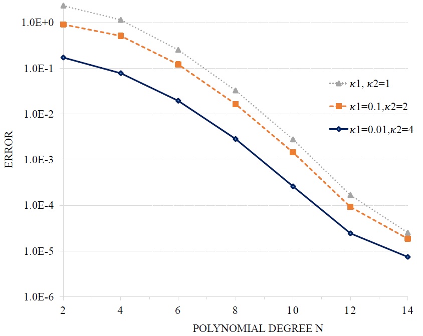
Figure 6.1: The $H^{1}$-error for some advection and dispersion coefficients for Example 2.

Example 3

Consider the problem (1.1) with $\kappa_{1}=0.2$ and $\kappa_{2}=1.5$ with the exact solution $u=x^{4}(1-x)^{2}t^{2}$. Table 3 shows the error results at $t=1$ for the fractional orders $\alpha=0.25$, $\alpha=0.50$ and $\alpha=0.75$.

Table 3: Errors for Example 3 at $t=1$ with CPU time (s).

		$\alpha=0.25$			$\alpha=0.5$			$\alpha=0.75$
$M$	$N$	$L_{\infty}^{T}$	$L_{2}^{T}$	time	$L_{\infty}^{T}$	$L_{2}^{T}$	time	$L_{\infty}^{T}$	$L_{2}^{T}$	time
40	4	9.49E-2	2.14E-1	2.45	8.57E-2	1.90E-1	1.98	7.62E-2	1.66E-1	2.47
80	6	3.01E-6	7.02E-6	5.94	1.86E-5	4.36E-5	5.78	9.56E-5	2.25E-4	5.58
160	8	1.35E-7	2.65E-7	17.66	9.26E-7	1.83E-6	17.00	5.38E-6	1.08E-5	17.37
320	10	4.22E-8	8.13E-8	53.88	3.35E-7	6.46E-7	49.27	2.27E-6	4.39E-6	52.86

Example 4

Consider the problem (1.1) with $\kappa_{1}=0.1$, $\kappa_{2}=2$ and the exact solution $u=x\cos(\frac{\pi}{2}x)\exp(-t)$. The rate of convergence in time is reported in Table 4 for $N=14$ at $t=1$. Also Fig. 6.2 illustrates the convergence in space for $\alpha=0.5$ and $\tau=1/100$ at $t=1$ in terms of $H^{1}-$norm.

The examples confirm the theoretical results of convergence of the time discretization (4.2) and spectral discretization (5.17).

Table 4: Experimental rate of convergence in time for Example 4 at $t=1$ with $N=14$.

	$\alpha=0.25$				$\alpha=0.5$				$\alpha=0.75$
$M$	$L_{\infty}^{T}$	rate	$L_{2}^{T}$	rate	$L_{\infty}^{T}$	rate	$L_{2}^{T}$	rate	$L_{\infty}^{T}$	rate	$L_{2}^{T}$	rate
25	1.68E-5		3.51E-5		7.87E-5		1.64E-4		3.04E-4		6.34E-4
50	5.12E-6	1.715	1.07E-5	1.715	2.79E-5	1.498	5.82E-5	1.497	1.27E-4	1.253	2.66E-4	1.252
100	1.55E-6	1.720	3.24E-6	1.720	9.87E-6	1.498	2.06E-5	1.498	5.35E-5	1.252	1.12E-4	1.251
200	4.71E-7	1.724	9.82E-7	1.723	3.50E-6	1.498	7.29E-6	1.498	2.25E-5	1.251	4.70E-5	1.251
400	1.42E-7	1.724	2.98E-7	1.722	1.24E-6	1.498	2.58E-6	1.498	9.45E-6	1.250	1.97E-5	1.254

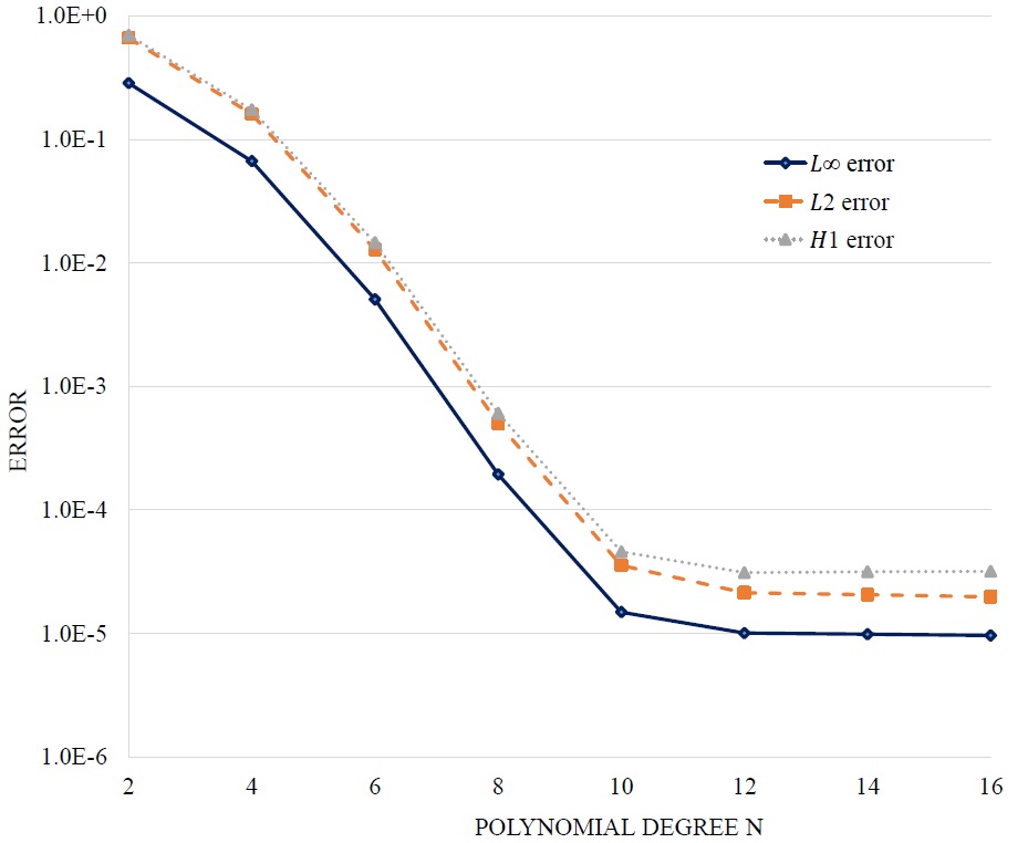
Figure 6.2: Convergence of the method for Example 4.

7 Conclusion

In this paper, we stated a new property for derivatives of Bernstein basis. Using this property, we obtained exact banded operational matrices for derivatives of Bernstein basis. Since the basis transformation may be ill-conditioned, the first advantage of our work in comparison with the existing works is that we did not use any basis transformation for the derivation of operational matrices. The second is that the derived matrices are banded, so less computational effort is required for a desired accuracy with less round-off errors. We also proposed a numerical method utilizing the Petrov-Galerkin method for the time-fractional advection dispersion equation on bounded domains based on the operational matrices leading to banded linear systems. Moreover, we derived the matrix formulation of the method and showed that the resulting linear system has a unique solution. We also discussed the error analysis. Then providing some numerical experiments, it is seen that the method is efficient, accurate and simple to implement for solving time-fractional advection dispersion equations on bounded domains.

References

- (1) Cheng, F.: On the rate of convergence of Bernstein polynomials of functions of bounded variation. J. Approx. Theory 39, 259-274 (1983)
- (2) Delgado, J., Pena, J.M.: Optimal conditioning of Bernstein collocation matrices. SIAM J. Matrix Anal. Appl 31, 990–996 (2009)
- (3) Deng, W.: Finite element method for the space and time fractional Fokker-Planck equation. SIAM J. Numer. Anal 47, 204-226 (2008)
- (4) Diethelm, K.: The analysis of fractional differential equations. Springer-Verlag, Berlin (2010)
- (5) Doha, E.H., Bhrawy, A.H., Saker, M.A.: On the derivatives of Bernstein polynomials: An application for the solution of high even-order differential equations. Boundary Value Problems 2011, 1-16 (2011) doi:10.1155/2011/829543
- (6) Farin, G.E., Hoschek, J., Kim, M.S.: Handbook of computer aided geometric design. Elsevier, Amsterdam (2002)
- (7) Farouki, R.T., Rajan, V.T.: Algorithms for polynomials in Bernstein form. Comput. Aided Geom. Des 5, 1-26 (1988)
- (8) Farouki, R.T.: On the stability of transformations between power and Bernstein polynomial forms. Comput. Aided Geom. Des 8, 29-36 (1991)
- (9) Farouki, R.T., Goodman, T.N.T.: On the optimal stability of the Bernstein basis. Math. Comput 64, 1553–1566 (1996)
- (10) Gao, G.H., Sun, H.W.: Three-point combined compact difference schemes for time-fractional advection–diffusion equations with smooth solutions. J. Comput. Phys 298, 520–538 (2015)
- (11) Golub, G.H., Ortega, J.M.: Scientific computing and differential equations: an introduction to numerical methods. Academic Press, San Diego (1992)
- (12) Jiang, Y., Ma, J.: High-order finite element methods for time-fractional partial differential equations. J. Comput. Appl. Math 235, 3285–3290 (2011)
- (13) Juttler, B.: The dual basis functions for the Bernstein polynomials. Adv. Comput. Math 8, 345–352 (1998)
- (14) Lin, Y., Chuanju X.: Finite difference/spectral approximations for the time-fractional diffusion equation. J. Comput. Phys 225, 1533-1552 (2007)
- (15) Maleknejad, K., Basirat, B., Hashemizadeh, E.: A Bernstein operational matrix approach for solving a system of high order linear Volterra–Fredholm integro-differential equations. Math. Comput. Modelling 55, 1363-1372 (2012)
- (16) Maleknejad, K., Hashemizadeh, E., Ezzati, R.: A new approach to the numerical solution of Volterra integral equations by using Bernstein’s approximation. Commun. Nonlinear Sci. Numer. Simulat 16, 647–655 (2011)
- (17) Pandey, R.K., Kumar, N.: Solution of Lane–Emden type equations using Bernstein operational matrix of differentiation. New Astronomy 17, 303-308 (2012)
- (18) Parand, K., Kaviani, S.A.: Application of the exact operational matrices based on the Bernstein polynomials. J. Math. Computer Sci 6, 36-59 (2013)
- (19) Ramezani, M., Mojtabaei, M., Mirzaei, D.: DMLPG solution of the fractional advection–diffusion problem. Eng. Anal. Bound. Elem 59, 36–42 (2015)
- (20) Saadatmandi, A.: Bernstein operational matrix of fractional derivatives and its applications. Appl. Math. Model 38, 1365–1372 (2014)
- (21) Saadatmandi, A., Dehghan, M.: A new operational matrix for solving fractional-order differential equations. Comput. Math. Appl 59, 1326–1336 (2010)
- (22) Shen, J., Tang, T., Wang, L.L.: Spectral methods: algorithms, analysis and applications. Springer-Verlag (2011)
- (23) Shirzadi, A., Ling, L., Abbasbandy, S.: Meshless simulations of the two-dimensional fractional-time convection–diffusion–reaction equations. Eng. Anal. Bound. Elem 36, 1522–1527 (2012)
- (24) Serre, D.: Matrices Theory and Applications. Grad. Texts in Math. 216, Springer-Verlag, New York (2002)
- (25) Stokes, P.W., Philippa, B., Read, W., White, R.D.: Efficient numerical solution of the time fractional diffusion equation by mapping from its Brownian counterpart. J. Comput. Phys 282, 334-344 (2015)
- (26) Yousefi, S.A., Behroozifar, M.: Operational matrices of Bernstein polynomials and their applications. Internat. J. Systems Sci 41, 709-716 (2010)
- (27) Yousefi, S.A., Behroozifar, M., Dehghan, M.: The operational matrices of Bernstein polynomials for solving the parabolic equation subject to specification of the mass. J. Comput. Appl. Math 17, 5272-5283 (2011)
- (28) Yüzbasi, S.: A collocation method based on Bernstein polynomials to solve nonlinear Fredholm–Volterra integro-differential equations. Appl. Math. Comput 273, 142–154 (2016)