Leading birds by their beaks: the response of flocks to external perturbations

Abstract

We study the asymptotic response of polar ordered active fluids (“flocks”) to small external aligning fields $h$. The longitudinal susceptibility $\chi_{{}_{\parallel}}$ diverges, in the thermodynamic limit, like $h^{-\nu}$ as $h\rightarrow 0$. In finite systems of linear size $L$, $\chi_{{}_{\parallel}}$ saturates to a value $\sim L^{\gamma}$. The universal exponents $\nu$ and $\gamma$ depend only on the spatial dimensionality $d$, and are related to the dynamical exponent $z$ and the “roughness exponent” $\alpha$ characterizing the unperturbed flock dynamics. Using a well supported conjecture for the values of these two exponents, we obtain $\nu=2/3$, $\gamma=4/5$ in $d=2$ and $\nu=1/4$, $\gamma=2/5$ in $d=3$. These values are confirmed by our simulations.

1 Introduction

Flocking – the collective motion of many active particles – is a ubiquitous emergent phenomenon that occurs in many living and synthetic systems over a wide range of scales. Examples range from mammal herds, fish schools and bird flocks to bacteria colonies and cellular migrations, down to subcellular molecular motors and biopolymers [1]. Over the last 20 years, studies of minimal models of self-propelled particles (SPP) [2, 3, 4, 5] and hydrodynamic continuum theories [6, 7, 8, 9, 10, 11, 12] have shown that the behavior of typical flocking systems is essentially determined by (i) the spontaneous breaking of continuous rotational symmetry and (ii) the far-from-equilibrium nature of locally interacting moving particles. While the former mechanism is common to many equilibrium systems (ranging from liquid crystals to magnetic systems and superfluid Helium-4 [13]) which spontaneously align a phase or orientational degree of freedom, the latter is unique to active matter systems. The self-propelled motion of active particles results in superdiffusive information propagation even in systems without momentum conservation, which in turn leads to many striking phenomena never found in equilibrium systems, such as long-range order in two spatial dimensions [6], and anomalously large number fluctuations [14].

However, little is known concerning the response of moving groups to external perturbations. This is an important question in statistical physics: symmetry breaking systems are often characterized by their response to a small external field, and studying response can also help answer the question of whether a generalized fluctuation-dissipation relation (FDR) of some sort [15] holds in flocks. Ethologists, on the other hand, are interested in response to external threats and more generally in the biological significance of group response mechanisms. Finally, understanding response is essential for controlling flocking systems, either biological or artificial.

In equilibrium, the response of systems breaking a continuous symmetry to a small external field is a classic problem of statistical field theory, first solved in [16], where it was shown that fluctuations transversal to order couple to longitudinal ones, yielding a diverging longitudinal susceptibility in the entire ordered phase. This is a typical manifestation of symmetry-breaking, and it is a natural question to wonder how the far-from-equilibrium nature of flocks may change this fundamental result.

Until now, only a few studies, mostly numerical, have addressed these questions. Asymptotic response has been first studied numerically in the well-known Vicsek model [3], but that work focused on the behavior of the susceptibility near the transition, rather than in the ordered phase. Short time response and the dynamic FDR has been investigated numerically in the Vicsek model [5] and in the isotropic phase of an active dumbbells system [17]. The response to finite and/or localized perturbations, finally, has also been studied in [18, 19, 20].

Here we provide a different approach, combining hydrodynamic theory results with numerical simulations to characterize the static response of ordered flocks to a small homogeneous external field of amplitude $h$.

We are particularly interested in the asymptotic longitudinal response

$$\chi_{\parallel}\equiv\frac{\delta\Phi(h)}{h}\,$$ (1)

where $\delta\Phi(h)=\Phi(h)-\Phi(0)$ is the change in the magnitude of the time-averaged order parameter, which in our case is the mean velocity, due to the applied field. Our main result is the scaling law:

$$\chi_{{}_{\parallel}}=h^{-\nu}f\left(Lh^{1\over z}\right)\propto\left\{\begin{array}[]{ll}h^{-\nu},&L\gg L_{c}(h)\\ L^{\gamma},&L\ll L_{c}(h)\end{array}\right.,$$ (2)

where $L_{c}(h)\propto h^{-1/z}$ and, using a conjecture first put forward in [6],

$$\nu={4-d\over d+1}\;,\;\;\;\;\;z={2(d+1)\over 5}\;,\;\;\;\;\;\gamma={2(4-d)\over 5}$$ (3)

for any dimension $3/2\leq d\leq 4$, the upper critical dimension. In particular, we have $\nu=2/3$, $z=6/5$ and $\gamma=4/5$ in $d=2$ and $\nu=1/4$, $z=8/5$ and $\gamma=2/5$ in $d=3$. For $d>4$, on the other hand, we predict $\delta\Phi\propto h$.

In the remainder of this paper, we will first derive the results (2) and (3) analytically, and then present numerical simulations that confirm them.

2 Response theory

We consider “dry” flocks, by which we mean flocks which move over a or through a static dissipative substrate or medium that acts as a momentum sink. Total momentum, thus, is not conserved, and no long ranged hydrodynamic interactions are present in the system. Obviously, Galilean invariance is broken, since the reference frame in which the static substrate or medium is at rest is preferred.

2.1 Hydrodynamic description

The hydrodynamic theory describes flocking by continuous, coarse grained number density $\rho({\bf r},t)$ and velocity ${\bf v}({\bf r},t)$ fields. The hydrodynamic equations of motion governing these fields in the long-wavelength limit can be obtained either by symmetry arguments [6, 7, 8, 9], or by kinetic theory [10, 11] and describe the asymptotic dynamics of polar flocks regardless of the precise nature of the interactions, provided only that they are local; in particular, the same hydrodynamic equations apply for both ”metric” and ”topological” interactions[21, 22]. They are

$$\partial_{t}\rho+\nabla\cdot({\bf v}\rho)=0$$ (4)

and, in a schematic notation

$$\partial_{t}{\bf v}+{\bf\Lambda}\left[{\bf\nabla}{\bf v}{\bf v}\right]=U(\rho,|{\bf v}|){\bf v}+{\bf D}\left[{\bf\nabla}{\bf\nabla}{\bf v}\right]+{\bf F_{P}}+{\bf f}+{\bf h}$$ (5)

where

$${\bf\Lambda}\left[{\bf\nabla}{\bf v}{\bf v}\right]\equiv\lambda_{1}({\bf v}\cdot{\bf\nabla}){\bf v}+\lambda_{2}({\bf\nabla}\cdot{\bf v}){\bf v}+\lambda_{3}{\bf\nabla}(|{\bf v}|^{2})$$ (6)

are all the convective-like terms permitted by the symmetries and conservation laws of the system. Here, all three coefficients are, in general, neither zero nor one, as opposed to systems with Galilean invariance where one has simply $\lambda_{1}=1$ and $\lambda_{2}=\lambda_{3}=0$ as in usual Navier-Stokes equations.
The viscous terms

$${\bf D}\left[{\bf\nabla}{\bf\nabla}{\bf v}\right]\equiv D_{1}{\bf\nabla}({\bf\nabla}\cdot{\bf v})+D_{2}({\bf v}\cdot{\bf\nabla})^{2}{\bf v}+D_{3}\nabla^{2}{\bf v}$$ (7)

reflect the tendency of localized fluctuations in the velocities to spread out because of local interactions.
The pressure term

$${\bf F_{P}}\equiv-{\bf\nabla}P_{1}-{\bf v}\left({\bf v}\cdot{\bf\nabla}P_{2}\right)$$ (8)

is the sum of an isotropic and anisotropic pressure terms, the latter being a genuinely non-equilibrium feature. Both terms tend to suppress local density fluctuations around the global mean value $\rho_{0}$. The pressures $P_{1,2}$, and the convective and viscous parameters $\lambda_{k}$ and $D_{k}>0$ ($k=1,2,3$) are functions of the local density $\rho$ and the magnitude $|{\bf v}|$ of the local velocity.
Fluctuations are introduced through a Gaussian white noise ${\bf f}$ with correlations

$$\left<f_{i}({\bf r},t)f_{j}({\bf r^{\prime}},t^{\prime})\right>=\Delta\delta_{ij}\delta^{d}({\bf r}-{\bf r^{\prime}})\delta(t-t^{\prime})$$ (9)

This accounts in a simple way for any source of microscopic fluctuations, such as the microscopic noise term opposing order in simple SPP models. Finally, the local term $U$ simply makes the local $\bf{v}$ have a nonzero magnitude $v_{0}(h)$ in the ordered phase. It satisfies the condition $U>0$ for $|{\bf v}|<v_{0}(h=0)$, $U=0$ for $|{\bf v}|=v_{0}(0)$, and $U<0$ for $|{\bf v}|>v_{0}(0)$. This term thereby spontaneously breaks rotational symmetry even in the absence of an external field. Small departures of the statistics of the noise from these assumptions, e.g., slightly non-Gaussian statistics, or the introduction of “local color” in the sense of short-ranged spatio-temporal correlations of the noise, change none of the long distance scaling properties of the flock.

Eqs. (4)-(5) are identical to the unperturbed ones discussed in [12], except for the explicit addition of the coarse-grained constant field ${\bf h}$ in Eq. (5). By analyticity and rotational invariance, this field is linearly and isotropically proportional to the applied microscopic field when those fields are sufficiently small.

2.2 Mean-field analysis

We first discuss the system in the absence of fluctuations. Eqs. (4)-(5) admit a spatially uniform steady state solution

$$\begin{array}[]{l}\rho({\bf r},t)=\rho_{0}\\ {\bf v}({\bf r},t)={\bf v}_{0}({\bf h})\end{array}$$ (10)

For any nonzero external field let $\hat{\bf e}_{\parallel}$ be the unit vector along ${\bf h}\equiv h\,\hat{\bf e}_{\parallel}$, while for strictly zero field $\hat{\bf e}_{\parallel}$ will be the direction of the spontaneous symmetry breaking. We have ${\bf v}_{0}({\bf h})=v_{0}(h)\hat{\bf e}_{\parallel}$, with the magnitude $v_{0}(h)$ of the homogeneous velocity ${\bf v}_{0}({\bf h})$ determined by the condition

$$U(v_{0}(h)),\rho_{0})\,v_{0}(h)+h=0\,.$$ (11)

Since $U$ is analytic in $v$, we have for small fields

$$v_{0}(h)-v_{0}(0)\propto h\,,$$ (12)

where $v_{0}(0)$ is the zero field symmetry broken solution. It is well known that sufficiently deep in the ordered phase such a zero-field solution is stable against spatial perturbations [11]. In the following we will restrict our analysis to this so-called Toner-Tu (TT) phase.
To summarize: in mean field theory, the magnitude of the order parameter

$$\Phi(h)\equiv|\langle{\bf v}({\bf r},t)\rangle|$$ (13)

(here and hereafter $\langle\cdot\rangle$ denotes a global average in space and time) responds linearly in $h$.

2.3 Fluctuations

We now move beyond mean field to consider the effect of fluctuations; we will show that the corrections to the order parameter $\Phi$ due to fluctuations are much larger than linear ones we’ve just computed at mean field level.

In order to do so, we allow for small fluctuations around the homogeneous solution,

$$\begin{array}[]{l}\rho({\bf r},t)=\rho_{0}+\delta\rho(h;{\bf r},t)\\ {\bf v}({\bf r},t)={\bf v}_{0}(h)+\delta{\bf v}(h;{\bf r},t)\,,\end{array}$$ (14)

and distinguish between longitudinal and transverse velocity fluctuations, which are respectively parallel ($\parallel$) and perpendicular ($\perp$) to ${\bf v}_{0}(h)$,

$$\delta{\bf v}(h;{\bf r},t)=\delta v_{\parallel}(h;{\bf r},t)\,{\bf e}_{\parallel}+{\bf v}_{\perp}(h;{\bf r},t)$$ (15)

where we have made explicit the field dependence of fluctuations. For simplicity, we will hereafter often not explicitly display the space, time and field dependence of the fluctuations.

Note that, due to number conservation, $\langle\delta\rho\rangle=0$, while symmetry considerations imply $\langle{\bf v}_{\perp}\rangle=\bf{0}$; that is, fluctuations can’t steer the global average of $\langle{\bf v}({\bf r},t)\rangle$ away from the external field direction. This implies that corrections to the order parameter are linear in the longitudinal fluctuations: By making use of Eqs. (12), (13) and (15) we have

$$\Phi(h)=v_{0}(h)+\langle\delta{\bf v}(h)\rangle=v_{0}(0)+\langle\delta v_{\parallel}(h)\rangle+O(h)$$ (16)

In order to compute longitudinal fluctuations, we have to expand the hydrodynamic equations (4)-(5) in the small fluctuations $\delta\rho$, $\delta v_{\parallel}$ and ${\bf v}_{\perp}$. We are interested only in fluctuations that vary slowly in space and time (indeed the hydrodynamic equations are only valid in this limit), so that space and time derivatives of the fluctuations are always of higher order than the fluctuations themselves. The details of this surprisingly subtle calculation are given in Appendix A, but (fortunately) they are identical to order $h$ with those for the zero-field case in Ref. [12]. The only difference at $O(h)$ is that

$$U(v_{0}(h),\rho_{0})\approx-\frac{h}{v_{0}}\neq 0\,.$$ (17)

Because slow modes dominate the long-distance behavior, and, it therefore proves, the small field response, we can eliminate the longitudinal fluctuations from Eqs. (22), since they are a fast mode of the dynamics. The subtle details of this elimination are given in Appendix A; the result is that the longitudinal velocity fluctuation becomes “enslaved” to the slow modes (that is, its instantaneous value is entirely determined by the instantaneous values of those slow modes) via the relation

$$\delta v_{\parallel}\approx-\frac{|{\bf v}_{\perp}(h)|^{2}}{2v_{0}(0)}+\mu_{1}\delta\rho+(\mu_{2}\partial_{t}+\mu_{3}\partial_{\parallel})\,\delta\rho+\mu_{4}\nabla_{\perp}\cdot{\bf v}_{\perp}+O(h)\,.$$ (18)

Here $\mu_{1}$ is a constant which depends on the form of $U$. In typical flocking models with metric interactions $\mu_{1}>0$ [11], so that density fluctuations are positively correlated with longitudinal fluctuations at the local level. In equation (18), $\nabla_{\perp}$ denotes spatial derivatives in the transverse directions, and the constants $\mu_{2}$, $\mu_{3}$ and $\mu_{4}$ depend on the original parameters of the hydrodynamic equations (4)-(5). Full details, together with the derivation of Eq. (18), can be found in Appendix A, but the exact form of these constants is unimportant here. Since these derivative terms are linear in $\delta\rho$ and ${\bf v}_{\perp}$, they vanish once averaged over space and time, so that from Eq. (18) we have

$$\langle\delta v_{\parallel}\rangle\approx-\frac{\langle|{\bf v}_{\perp}(h)|^{2}\rangle}{2v_{0}(0)}+O(h)$$ (19)

which links the global average of transversal and longitudinal fluctuations and is the analogous of the so-called principle of conservation of the modulus in an equilibrium ferromagnet [16]. From Eq. (16) we finally have

$$\Phi(h)\approx v_{0}(0)-\frac{\langle|{\bf v}_{\perp}(h)|^{2}\rangle}{2v_{0}(0)}+O(h)$$ (20)

and

$$\delta\Phi(h)\equiv\Phi(h)-\Phi(0)\approx\frac{\langle|{\bf v}_{\perp}(0)|^{2}\rangle-\langle|{\bf v}_{\perp}(h)|^{2}\rangle}{2v_{0}(0)}+O(h)$$ (21)

We are then left with the problem of determining the fluctuations of the transverse velocity ${\bf v}_{\perp}$ in the presence of a non-zero field $h$. We will do so by analyzing the equations of motion for ${\bf v}_{\perp}$ and $\delta\rho$, which follow from inserting (18) into the velocity equation of motion (5) projected transverse to the direction of mean motion, and into the density equation of motion (4), and expanding in fields and derivatives. Again, details are relegated to Appendix A; the result is:

$$\partial_{t}\delta\rho = \left[\,\partial_{t}\delta\rho\,\right]_{h=0}$$ (22)

$$\partial_{t}{\bf v}_{\perp} = \left[\,\partial_{t}{\bf v}_{\perp}\right]_{h=0}-h_{v}{\bf v}_{\perp}$$

where we have introduced the rescaled field

$$h_{v}\equiv\frac{h}{v_{0}(0)}$$ (23)

and $\left[\,\partial_{t}\delta\rho\,\right]_{h=0}$ and $\left[\,\partial_{t}{\bf v}_{\perp}\right]_{h=0}$ are the terms originally given by Eqs. (2.18) and (2.28) of [12] for the zero field case. For later use, we denote collectively the parameters appearing in those terms as $\{\mu_{i}^{(0)}\}$. While the exact forms of Eqs. (22) are not important for what follows, for completeness we also give them in Appendix A.

2.4 Renormalization Group

We have shown so far that the response $\delta\Phi$ is determined by the global average of transversal fluctuations, Eq. (21). To compute this quantity, we proceed by a dynamical renormalization group (DRG) analysis [23] of Eqs. (22). Once again, this standard analysis is almost identical to that carried out in [12] for the zero field case. We start by averaging the equations of motion over the short-wavelength fluctuations: i.e., those with support in the “shell” of Fourier space $b^{-1}\Lambda\leq|{\bf q}_{{}_{\perp}}|\leq\Lambda$, where $\Lambda$ is an “ultra-violet cutoff”, and $b$ is an arbitrary rescaling factor. Then, one rescales lengths, time, $\delta\rho$ and ${\bf v}_{{}_{\perp}}$ in equations (22) according to ${\bf v}_{{}_{\perp}}=b^{\alpha}{\bf v}_{{}_{\perp}}^{\,\prime}$, $\delta\rho=b^{\alpha}\delta\rho^{\,\prime}$, ${\bf r}_{{}_{\perp}}=b{\bf r}_{\perp}^{\,\prime}$, $r_{{}_{\parallel}}=b^{\zeta}r^{\prime}_{{}_{\parallel}}$, and $t=b^{z}t^{\prime}$ to restore the ultra-violet cutoff to $\Lambda$ . The scaling exponents $\alpha$, $\zeta$, and $z$, known respectively as the “roughness”, “anisotropy”, and “dynamical” exponents, are at this point arbitrary.

This DRG process leads to a new, “renormalized” pair of equations of motion of the same form as (22), but with “renormalized” values of the parameters, $\{\mu_{i}^{(0)}\}\to\{\mu_{i}^{(b)}\}$. For a suitable choice of the scaling exponents $\alpha$, $\zeta$, and $z$, these parameters flow to fixed, finite limits as $b\rightarrow\infty$; that is, $\{\mu_{i}^{(b\rightarrow\infty)}\}\rightarrow\{\mu_{i}^{*}\}$; this is referred to as a “renormalization group fixed point”. The utility of this choice will be discussed in a moment.

Since all terms except the $h$ term in Eqs. (22) are rotation invariant, they can only generate other rotation invariant terms in the first (averaging) step of the DRG. Hence, they cannot renormalize $h$, which breaks rotation invariance. Thus, the only change in the $h$ term in Eqs. (22) occurs in the second (rescaling) step. Since the coefficient $h_{v}$ scales as the inverse of time, this is easily seen to lead to the recursion relation

$$h_{v}=b^{-z}h_{v}^{\prime}~{}~{},$$ (24)

which – for the reasons just given – is exact to linear order in $h$.

By construction, the DRG has the property that correlation functions in the original equations of motions can be related to those of the renormalized equations of motion via a simple scaling law. The example of interest for our problem is of course the correlation function

$$C\left(L_{\perp},L_{\parallel},\{\mu_{i}^{0}\},h_{v}\right)\equiv\langle|{\bf v}_{\perp}(0)|^{2}\rangle-\langle|{\bf v}_{\perp}(h)|^{2}\rangle$$ (25)

Here $L_{\perp}$ and $L_{\parallel}$ are respectively the transverse and longitudinal system size. The DRG scaling law obeyed by $C$ is thus

$$C\left(L_{\perp},L_{\parallel},\{\mu_{i}^{0}\},h_{v}\right)=b^{2\alpha}C\left(b^{-1}L_{\perp},b^{-\zeta}L_{\parallel},\{\mu_{i}^{b}\},b^{z}h_{v}\right)$$ (26)

which follows simply from the fact that $C$ involves two powers of ${\bf v}_{\perp}$, each of which gives a factor $b^{\alpha}$.

In order to examine the scaling of $C$ with field amplitude $h$, we use the completely standard[23, 24] renormalization group trick of choosing the scaling factor $b$ such that $b^{z}h_{v}$ is equal to some constant reference field strength $h_{v}^{*}$, which we will always choose to have the same value regardless of the bare value of $h_{v}$. This implies that $b=\left({h_{v}\over h_{v}^{*}}\right)^{-1/z}$. Note that for small $h$ – and thus small $h_{v}$ – this choice implies $b\gg 1$, and that the parameters $\{\mu_{i}^{(b)}\}$ flow to $\{\mu_{i}^{*}\}$, their fixed point values. Hence, in the limit of small $h$, the scaling function (26) can be reduced to

$$C(L_{\perp},L_{\parallel},\{\mu_{i}^{0}\},h)=h^{-2\alpha/z}g(L_{\perp}h^{1/z},L_{\parallel}h^{\zeta/z})$$ (27)

where

$$g(x,y)\equiv b_{0}^{2\alpha/z}C(b_{0}^{-1/z}x,b_{0}^{-\zeta/z}y,\{\mu_{i}^{*}\},h_{v}^{*})\,\;\;\;\;\mbox{with}\;b_{0}\equiv h_{v}^{*}\,v_{0}(0)\,,$$ (28)

is a universal scaling function (since we always make the same choice of $h_{v}^{*}$).

Note that this expression only applies for small $h$, since it is only in that limit that $b\rightarrow\infty$, and, hence $\{\mu_{i}^{(b)}\}\rightarrow\{\mu_{i}^{*}\}$. Hence, we expect this scaling law to break down for large fields, and, in fact, it does.

We now focus our attention on roughly square systems, with $L_{\perp}\sim L_{\parallel}\sim L$. Assuming an anisotropy exponent $0<\zeta<1$ (as expected [6, 7, 8, 9, 12] for spatial dimensions $d<4$), we have for small fields

$$Lh^{1/z}\propto L_{\perp}h^{1/z}\ll L_{\parallel}h^{\zeta/z}$$ (29)

so that finite-size scaling is controlled by the transverse flock extension $L_{\perp}$ and we can replace $g$ with the universal scaling function $w(x)\equiv g(x,\infty)$. Above the upper critical dimension $d_{c}=4$, where $\zeta=1$ [6], scaling is the same in both the transversal and longitudinal directions and we choose instead $w(x)\equiv g(x,x)$. Doing so, we finally obtain the scaling law

$$C(L,h)=h^{1-\nu}\tilde{w}(Lh^{1/z})$$ (30)

where

$$\nu=1+2\alpha/z\,.$$ (31)

It is now straightforward to relate the order parameter change $\delta\Phi(h)$ to this scaling law. From Eq. (21) we have

$$\delta\Phi\propto C(L,h)+O(h)\,.$$ (32)

Note that for $\nu>0$ (again a condition we expect, as discussed below, to be satisfied for $d<4$), we have $C(L,h)\gg O(h)$ and the corrections due to fluctuations dominate the mean field ones. To lowest order in $h$

$$\delta\Phi=\frac{1}{2v_{0}(0)}\left[\langle|{\bf v}_{\perp}(0)|^{2}\rangle-\langle|{\bf v}_{\perp}(h)|^{2}\rangle\right]=h^{1-\nu}w(Lh^{1/z})$$ (33)

In the thermodynamic limit, $Lh^{1/z}\gg 1$ for any non-zero field and $w(Lh^{1/z})\rightarrow w(\infty)=\rm{constant}$, yielding the asymptotic result ${\delta\Phi\over h}\propto h^{-\nu}$. In practice, in any system large enough, the external field suppresses transverse fluctuations, thus increasing the scalar order parameter according to Eq. (20), an effect that below the upper critical dimension $d_{c}=4$ proves stronger than mean field corrections linear in $h$. Above $d_{c}$, on the other hand, it is known [6] that $\alpha=1-d/2$ and $z=2$, which implies $\nu=2-d/2\leq 0$; therefore corrections due to fluctuations no longer dominate the mean field ones. Hence, ordinary linear response $\chi_{\parallel}\rightarrow\rm{constant}$ as $h\rightarrow 0$ is recovered for $d>4$.

So far, we have kept our discussion of DRG at a qualitative level, independent of the precise form of the zero-field terms in Eqs. (22). To be more quantitative for $d<4$, we need the actual values of the scaling exponents $\alpha$, $\zeta$, and $z$ for which the DRG flows to a fixed point in those dimensions. These values actually do depend on the form of Eqs. (22) (and, in particular, to the nature of their relevant nonlinear terms), but luckily for small fields $h$ they have to coincide with their zero-field values. Indeed, there is no reason for which these zero-field values should be affected by a sufficiently small rescaled field, $h_{v}\leq h_{v}^{*}$.

In [6], it was argued that for any dimension $3/2\leq d\leq 4$ these zero-field exponents are

$$\alpha={3-2d\over 5}\;,\;\;\;\;z={2(d+1)\over 5}\;,\;\;\;\;\ \zeta={d+1\over 5}.$$ (34)

It has since been since realized [12] that the original arguments leading to these values are flawed. However, the simple conjecture that the only relevant non-linearity at the fixed point is the term proportional to $\lambda_{1}$ in Eqs. (5)-(6) leads to precisely these values for the exponents. While this conjecture has never been proven, there is solid numerical [5, 7] and even experimental [25] evidence supporting the above scaling exponent values for $d=2$ and, to a lesser extent, $d=3$. In the following we will assume this conjecture holds, verifying it a-posteriori by numerical measures of asymptotic response in the Vicsek [2] model.

Above the upper critical dimension, $d_{c}=4$, finally, the scaling exponents take the exact linear values $z=2$, $\zeta=1$ and $\alpha=1-d/2$.

2.5 Finite size effects and longitudinal response

We conclude this section discussing finite size effects. The scaling form (33) implies that transverse fluctuations are suppressed by the field $h$ on length scales

$$L\gg L_{c}(h)\propto h^{-1/z}\,.$$ (35)

In small systems such that $L\ll L_{c}$ (or equivalently for small field $h\ll h_{c}(L)\propto L^{-z}$), however, this suppression is ineffective, and leading corrections to the order parameter should revert to linear order in the external field $h$. We can include this behavior in a single universal scaling function $f$ by requiring that $f(\infty)\propto w(\infty)=O(1)$ and $f(x)\propto x^{\nu z}$ for $x\ll 1$. This finally gives,

$$\delta\Phi=h^{1-\nu}f\left(h\,L^{z}\right)\propto\left\{\begin{array}[]{ll}h^{1-\nu},&h\gg L^{-z}\\ hL^{\gamma},&h\ll L^{-z}\end{array}\right..$$ (36)

with $\gamma=\nu z$. This scaling holds for external fields not too large. For $h>h_{v}^{*}$, on the other hand, the small field approximation discussed here is no longer valid, and saturation effects change the scaling (36). Once expressed in terms of the longitudinal susceptibility $\chi_{\parallel}=\delta\Phi/h$, our results imply Eq. (2), with the scaling exponents given by Eq. (3) (according to conjecture (34)).

3 Numerical simulations

We test our predictions (36) in two and three dimensions by simulating the well known Vicsek model [2] in an external homogeneous field ${\bf h}$. Each particle – labeled by $i=1,2,\ldots,N$ – is defined by a position ${\bf r}_{i}^{t}$ and a unit direction of motion ${\bf v}_{i}^{t}$. The model evolves with a synchronous discrete time dynamics

$${\bf v}_{i}^{t+1} = (\mathcal{R}_{\omega}\circ\vartheta)\left(\sum_{j\in S_{i}}{\bf v}_{j}^{t}+{\bf h}\right)$$ (37)

$${\bf r}_{i}^{t+1} = {\bf r}_{i}^{t}+v_{m}{\bf v}_{i}^{t}$$ (38)

where $v_{m}$ is the particle speed, $\vartheta({\bf w})={\bf w}/|{\bf w}|$ is a normalization operator and $\mathcal{R}_{\omega}$ performs a random rotation (uncorrelated between different times $t$ or particles $i$) uniformly distributed around the argument vector: $\mathcal{R}_{\omega}{\bf w}$ is uniformly distributed around ${\bf w}$ inside an arc of amplitude $2\pi\omega$ (in $d=2$) or in a spherical cap spanning a solid angle of amplitude $4\pi\omega$ ($d=3$). The interaction is “metric”: that is, each particle $i$ interacts with all of its neighbors within unit distance. In the following, we adopt periodic boundary conditions and choose typical microscopic parameters so that the system lies within the TT phase [5]: $v_{m}=0.5$, $\rho_{0}=N/L^{d}=1$ and $\omega=0.18$ ($d=2$) or $\omega=0.11$ ($d=3$). In both dimensions, this choice yields a zero-field order parameter $\Phi(0)\approx 0.8$.

We perform simulations with different external field amplitudes and with different linear system sizes $L$. After discarding a transient $T_{0}$ sufficiently long for the system to settle into the stationary state, we estimate the mean global order parameter

$$\Phi=\left\langle\frac{1}{N}\left|\sum_{i=1}^{N}{\bf v}_{i}^{t}\right|\right\rangle_{t}$$ (39)

and its standard error, given by $S_{E}=\sigma/\sqrt{n}$, with $\sigma$ being the standard deviation and $n$ the number of independent data points. We estimate $n$ as the total number of stationary points $T$ divided by the autocorrelation time $\tau$ of the mean order parameter timeseries, $n=T/\tau$. In Eq. (39), $\langle\cdot\rangle_{t}$ denotes time averages, performed over typically $T=10^{6}\sim 10^{8}$ time steps. In particular, as the precision of the zero-field order parameter affects all response and the autocorrelation time decreases with $h$, in our numerical simulations we take care to estimate the zero-field order parameter over times as large as possible.

We begin addressing response in the large system size (or large field) regime $hL^{z}\gg 1$, where our theory predicts $\delta\Phi\sim h^{1-\nu}$. Measuring this power law is a particularly difficult task, as it is sandwiched between saturation effects at larger values of $h$ and the crossover to linear behavior at $h\ll L^{-z}$. We proceed by extrapolation, choosing a (somewhat arbitrary) $h$ range of two decades and by measuring the effective power law exponent $1-\nu_{eff}$ by linear regression. The resulting response $\delta\Phi(h)$ is plotted in Fig. 1 for increasing system sizes $L$. As one expects, as system sizes increases, response curves approach the expected size-asymptotic behavior $\delta\Phi\sim h^{1-\nu}$. In Fig. 1a, for instance, the $d=2$ response approaches the expected power-law $1-\nu=1/3$. In the inset of Fig. 1a we further quantify this convergence plotting $|\nu_{eff}-\nu|$ vs. the system size $L$. This shows that the effective exponent approaches the predicted one with corrections of order $1/\sqrt{L}$. We repeated the same procedure in $d=3$. As shown in Fig. 1b, the approach to the expected asymptotic exponent $1-\nu=3/4$ is faster, and the difference $|\nu_{eff}-\nu|$ vanishes faster, as $L^{-1.5}$. In $d=3$ our simulations are obviously limited to a much smaller range of linear size values, but it should be noted that in $d=3$ finite size effects vanish quicker (being the exponent $z$ larger) while the asymptotic exponent $1-\nu=3/4$ is already quite close to the value $\delta\Phi\sim h$ expected at low values of $h$. A faster approach of $\nu_{eff}$ to its asymptotic value is therefore not completely surprising.

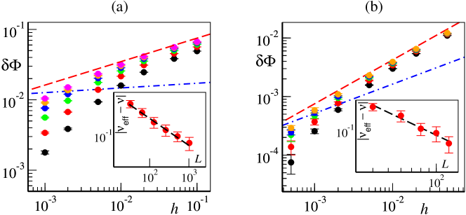
Figure 1: (color online) Size-asymptotic regime – Order parameter change vs. the applied field amplitude for different system sizes. a) For $d=2$, from bottom to top, $L=32,64,128,256,512,1024$. The dashed red line marks the expected asymptotic power law behavior $\delta\Phi\sim h^{1/3}$, while the dashed blue line marks the upper bound for the $d=2$ equilibrium response $\delta\Phi\sim h^{1/15}$. In the inset: Absolute difference between the measured effective exponent $\nu_{eff}$ (see text) and its expected asymptotic value $\nu$ as a function of system size. The dashed black lines marks a power law decay as $1/\sqrt{L}$. (b) For $d=3$, from bottom to top, $L=40,60,80,100,120$. The dashed red line marks the expected asymptotic power law behavior $\delta\Phi\sim h^{3/4}$, while the dashed blue line correspond to the $d=3$ equilibrium response $\delta\Phi\sim h^{1/2}$. Inset: $d=3$ data as in the inset of panel (a). The dashed black lines marks a power law decay as $L^{-1.5}$. Error bars measure standard errors (see text). All graphs are in a double logarithmic scale.

In $d=3$, we can also easily compare the response behavior with the equilibrium prediction $\delta\Phi\sim\sqrt{h}$ [16] (dashed blue line in Fig. 1b). This clearly shows that the far-from-equilibrium nature of the Vicsek model makes the susceptibility exponent very different from that in equilibrium ferromagnets. In $d=2$ equilibrium systems with a continuous symmetry cannot develop long range order, but, rather, exhibit only a quasi-long range ordered phase, characterized by scaling exponents that vary continuously with temperature [13, 27]. The equilibrium susceptibility exponent [27, 28] in $d=2$ is given by

$$\nu={4-2\eta\over 4-\eta}\,,$$ (40)

where the order parameter correlation exponent $\eta$ is bounded: $0\leq\eta\leq 1/4$, which implies that the susceptibility exponent $\nu$ varies over an extremely narrow range: $14/15\leq\nu\leq 1$. Our predicted value of $\nu=2/3$ for 2d flocks lies well outside this range; far enough, in fact, that our simulations both support the theory presented here, and rule out any equilibrium interpretation.

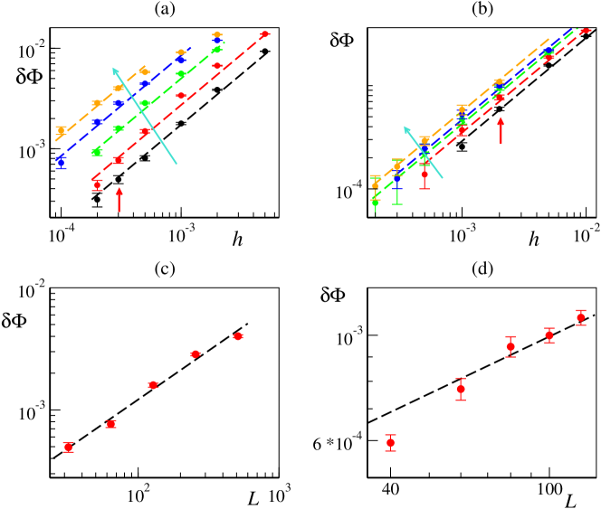
Figure 2: (color online) Linear regime. (a)-(b) Order parameter change vs. the applied field amplitude in the linear regime for different system sizes (the cyan arrow indicates increasing system sizes): a) For $d=2$ $L=32,64,128,256,512$. (b) For $d=3$ $L=40,60,80,100,120$. The dashed lines mark the linear relation $\delta\Phi\sim h$. Error bars measure data standard errors (see text). (c) $d=2$ Response at fixed $h$ – as shown by the red arrows in panel (a) – and different system sizes in the linear regime. The dashed black line marks a power law with the predicted slope $0.8$. (d) Same as in (c), but for $d=3$. The dashed black line marks a power law with the predicted slope $0.4$. All graphs are in a double logarithmic scale.

Next, we consider the linear behavior $\delta\Phi\propto h$ predicted for small system sizes (or small fields), $hL^{z}\ll 1$. This inequality imposes a (severe) upper limit on the range of $h$, while there is a lower limit set by our numerical precision in evaluating responses of the order of $10^{-4}$ or smaller. Nevertheless, our numerical simulations reveal in both $d=2$ (Fig. 2a) and $d=3$ (Fig. 2b) a linear growth of the response over more than one decade in the field amplitude $h$, especially for small system sizes.

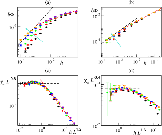
Figure 3: (color online) (a)-(b) Order parameter change vs. the applied field amplitude in both the linear and size-asymptotic regimes for different system sizes (the arrow indicates increasing system sizes): a) For $d=2$ $L=32,64,128,256,512,1024$. (b) For $d=3$ $L=40,60,80,100,120$. (c)-(d) data collapse for the longitudinal susceptibility according to Eq. (2) and to the conjectured values for the scaling exponents (see text). (c) $d=2$ and (d) $d=3$. In all panels, the dashed black lines mark the linear response ($\delta\Phi\propto h$ or $\chi_{\parallel}\sim L^{\gamma}$ expected by our theory for $h\ll h_{c}\sim L^{-z}$. Dashed red lines, on the other hand, mark the nonlinear regime predicted for $h\gg h_{c}$, $\delta\Phi\propto h^{1-\nu}$ or $\chi_{\parallel}\propto h^{-\nu}$. We have $\nu(d=2)=2/3$, and $\nu(d=3)=1/4$. Error bars measure standard errors (see text). All graphs are in a double logarithmic scale.

By selecting a single $h$ value lying in the linear regime for all accessible system sizes $L$, one is also able to test the saturation exponent gamma, $\delta\Phi\sim h\,L^{\gamma}$. This is done in Figs. 2c-d, where response values at different linear sizes $L$ are compared to the predicted power-law with (respectively) $\gamma=4/5$ for $d=2$ and $\gamma=2/5$ in $d=3$. We obtain a good agreement in $d=2$ (the best linear fit being $\gamma=0.79(5)$, while data in $d=3$ is less clear, in rough agreement with the expected power-law behavior only for sizes $L\geq 60$, with a best linear fit of $\gamma=0.48(7)$.

We finally consider the full range of accessible external fields values in Fig. 3a-b, which shows data for the accessible range of external field values in both two and three dimensions. Fields $h$ larger than $h_{s}\approx 0.1$, of course, are out of the small field regime and show saturation effects, while due to statistical fluctuations we have been unable to obtain reliable estimates for external fields smaller than $h\approx 10^{-4}$. Within this range, comparison with the predicted scaling (2) (as given by the dashed lines) is overall satisfactory, especially in $d=2$. By a proper rescaling, making use of the three scaling exponents (3), we can also collapse our data at different sizes on roughly a single curve, as shown in Fig. 3c-d.

To summarize, numerical simulations are in good agreement with our theoretical predictions, at least in $d=2$. Results in $d=3$ are prone to larger errors and obviously explore a more limited range of linear sizes, but nevertheless are still compatible with our predictions.

We also performed a few additional numerical studies of response (not shown here) with different parameter values (but still in the TT phase), and in the ordered phase of the so-called topological Vicsek model [29], confirming the generality of these results.

It is also worth commenting on the way the external field is implemented in the microscopic Vicsek equations (38). In Ref. [5] it was argued that different microscopic implementations could lead to different response, and in particular it was recommended to choose one by which the external field was normalized by the local order parameter value, such as in

$${\bf v}_{i}^{t+1}=(\mathcal{R}_{\omega}\circ\vartheta)\left[\vartheta\left(\sum_{j\in S_{i}}{\bf v}_{j}^{t}\right)+{\bf h}\right]$$ (41)

However, we do not expect these microscopic details to change the structure of the hydrodynamic equations (4)-(5), and thus we do not expect qualitative differences between the two microscopic external field implementations. Indeed, our preliminary simulations of Eq. (41) (not shown here) show no qualitative difference from the response extensively discussed above for Eq. (38).

4 Conclusions

So far, we have only considered the longitudinal susceptibility, which characterizes the response of the magnitude of the order parameter to a small external field. Simple considerations, based on symmetry, imply that the flock polarization vector will eventually align with any non-zero stationary external field, including one applied transversal to the initial polarization. Thus, for the transvere susceptibility we have, trivially,

$$\chi_{\perp}\sim\frac{v_{0}(0)}{h}$$ (42)

as in equilibrium systems.

In this paper, we have fully characterized the static response of homogeneous ordered flocks to small external fields for any dimension $d>3/2$. In particular, below the upper critical dimension $d_{c}=4$, our results in the thermodynamic limit $L\to\infty$ show a diverging longitudinal response for $h\to 0$, i.e. a diverging susceptibility. This is ultimately a consequence of the spontaneous symmetry breaking of the continuous rotation symmetry, albeit the far-from equilibrium nature of flocks yields different results from, say, equilibrium ferromagnets in $d=2,3$ [13]. We have also fully characterized finite size effects – typically of great importance in biological applications of collective motion – and verified our results via numerical simulations. We believe that the finite numerical values reported in Ref. [3] for the longitudinal susceptibility are entirely due to finite size effects.

Incidentally, our numerics thereby also provide further evidence supporting the conjecture (34) for the scaling exponent values [6].

Our results are expected to hold generically for all collective motion systems showing a bona fide TT phase. This class encompasses both systems with metric interactions and those with topological interactions. It also includes the inertial spin model recently put forward in [30] to account for the turning dynamics measured experimentally in starling flocks. This is because the long time hydrodynamic theory of the inertial spin theory relaxes to the TT theory [31]; hence, the static response will be unchanged. Dynamical response (i.e. how quickly the flock turns towards the field direction), however, could be different at short times in inertial spin models, while the long-time behavior should be the same.

In future work, we will explore more thoroughly the phase diagram of Vicsek-like models beyond the TT phase, investigating the disordered and phase separated regimes Other future directions include the study of the finite-time, dynamical reponse [32] in both overdamped Vicsek-like models and inertial spin ones, and the study of spatially localized perturbations.

Appendix A Expansion of the Hydrodynamic equations for small fluctuations

We first demonstrate that the longitudinal velocity $\delta v_{\parallel}$ is enslaved to the slow modes $\delta\rho$ and ${\bf v}_{\perp}$. We follow Ref. [12] and begin with the hydrodynamic Eqs. (4) and (5) written out explicitly:

$$\partial_{t}\rho+\nabla\cdot({\bf v}\rho)=0$$ (43)

$$\partial_{t}{\bf v} = -\lambda_{1}({\bf v}\cdot{\bf\nabla}){\bf v}-\lambda_{2}({\bf\nabla}\cdot{\bf v}){\bf v}-\lambda_{3}{\bf\nabla}(|{\bf v}|^{2})+U(\rho,{\bf v}){\bf v}-{\bf\nabla}P_{1}$$

$$- {\bf v}\left({\bf v}\cdot{\bf\nabla}P_{2}\right)+D_{1}{\bf\nabla}({\bf\nabla}\cdot{\bf v})+D_{3}\nabla^{2}{\bf v}+D_{2}({\bf v}\cdot{\bf\nabla})^{2}{\bf v}+{\bf f}+{\bf h}\,,$$

where, as noted in the main text, the parameters $\lambda_{i}(i=1\to 3)$, the local term $U$, the “isotropic Pressure” $P(\rho,|{\bf v}|)$ and the “anisotropic Pressure”$P_{2}(\rho,|{\bf v}|)$ are, in general, functions of the density $\rho$ and the magnitude $|{\bf v}|$ of the local velocity. It is useful to Taylor expand $P_{1}$ and $P_{2}$ around the equilibrium density $\rho_{0}$:

$$P_{1}=\sum_{n=1}^{\infty}\sigma_{n}(|{\bf v}|)(\rho-\rho_{0})^{n}$$ (45)

$$P_{2}=P_{2}(\rho,|{\bf v}|)=\sum_{n=1}^{\infty}\Upsilon_{n}(|{\bf v}|)(\rho-\rho_{0})^{n}~{}~{}.$$ (46)

Here $D_{1}$, $D_{2}$ and $D_{3}$ are all positive in the ordered state.
Again as discussed in the main text, in the ordered phase, the velocity field can be written as:

$${\bf v}=v_{0}{\bf{e}}_{{{}_{\parallel}}}+{\bf\delta v}=(v_{0}+\delta v_{{}_{\parallel}}){\bf e}_{{{}_{\parallel}}}+{\bf v}_{\perp}~{}~{}$$ (47)

(for simplicity, here and hereafter, we write $v_{0}\equiv v_{0}(h)$).
Taking the dot product of both sides of equation (LABEL:EOM) with ${\bf v}$ itself, we obtain:

$${1\over 2}\left(\partial_{t}|{\bf v}|^{2}\right) + {1\over 2}\left(\lambda_{1}+2\lambda_{3})({\bf v}\cdot{\bf\nabla})|{\bf v}|^{2}\right)+\lambda_{2}({\bf\nabla}\cdot{\bf v})|{\bf v}|^{2}=U(|{\bf v})|{\bf v}|^{2}$$

$$- {\bf v}\cdot{\bf\nabla}P_{1}-|{\bf v}|^{2}{\bf v}\cdot{\bf\nabla}P_{2}+D_{1}{\bf v}\cdot{\bf\nabla}({\bf\nabla}\cdot{\bf v})+D_{3}{\bf v}\cdot\nabla^{2}{\bf v}$$

$$+ D_{2}{\bf v}\cdot\left(({\bf v}\cdot{\bf\nabla})^{2}{\bf v}\right)+{\bf v}\cdot{\bf f}+{\bf v}\cdot{\bf h}~{}.$$

In this hydrodynamic approach, we are interested only in fluctuations ${\bf\delta v}({\bf r},t)$ and $\delta\rho({\bf r},t)$ that vary slowly in space and time. (Indeed, the hydrodynamic equations (LABEL:EOM) and (43) are only valid in this limit). Hence, terms involving space and time derivatives of ${\bf\delta v}({\bf r},t)$ and $\delta\rho({\bf r},t)$ are always negligible, in the hydrodynamic limit, compared to terms involving the same number of powers of fields without any time or space derivatives.

Furthermore, the fluctuations ${\bf\delta v}({\bf r},t)$ and $\delta\rho({\bf r},t)$ can themselves be shown to be small in the long-wavelength limit [12]. Hence, we need only keep terms in equation (LABEL:v_parallel_elim) up to linear order in ${\bf\delta v}({\bf r},t)$ and $\delta\rho({\bf r},t)$. The ${\bf v}\cdot{\bf f}$ term can likewise be dropped, since it only leads to a term of order ${\bf v}_{{}_{\perp}}f_{{}_{\parallel}}$ in the ${\bf v}_{{}_{\perp}}$ equation of motion, which is negligible (since ${\bf v}_{{}_{\perp}}$ is small) relative to the ${\bf f}_{\perp}$ term already there.

In addition, treating the magnitude $h$ of the applied field as a small quantity, we need only keep terms involving $h$ that are proportional to $h$ and independent of the small fluctuating quantities ${\bf\delta v}$ and $\delta\rho$.

These observations can be used to eliminate many of the terms in equation (LABEL:v_parallel_elim), and solve for the quantity $U$; the solution is:

$$U=-{h\over v_{0}}+\lambda_{2}{\bf\nabla}\cdot{\bf v}+{\bf v}\cdot{\bf\nabla}P_{2}+{\sigma_{1}\over v_{0}}\partial_{{}_{\parallel}}\delta\rho+{1\over 2v_{0}}\left(\partial_{t}+\lambda_{4}\partial_{{}_{\parallel}}\right)\delta v_{{}_{\parallel}},$$ (49)

where we’ve defined

$$\lambda_{4}\equiv(\lambda_{1}+2\lambda_{3})v_{0}~{}.$$ (50)

We can now express the longitudinal velocity $\delta v_{\parallel}$ in terms of the slow modes using equation (49) and the expansion

$$U\approx-\Gamma_{1}\left(\delta v_{{}_{\parallel}}+{|{\bf v}_{{}_{\perp}}|^{2}\over 2v_{0}}\right)-\Gamma_{2}\delta\rho~{}~{},$$ (51)

where we’ve defined

$$\Gamma_{1}\equiv-\left({\partial U\over\partial|{\bf v}|}\right)^{0}_{\rho} \Gamma_{2}\equiv-\left({\partial U\over\partial\rho}\right)^{0}_{|{\bf v}|}~{},$$ , (52)

with, here and hereafter, super- or sub-scripts $0$ denoting functions of $\rho$ and $|{\bf v}|$ evaluated at $\rho=\rho_{0}$ and $|{\bf v}|=v_{0}$. We’ve also used the expansion (47) for the velocity in terms of the fluctuations $\delta v_{{}_{\parallel}}$ and $\vec{v}_{\perp}$ to write

$$|{\bf v}|=v_{0}+\delta v_{{}_{\parallel}}+{|{\bf v}_{{}_{\perp}}|^{2}\over 2v_{0}}+O(\delta v_{{}_{\parallel}}^{2},|{\bf v}_{{}_{\perp}}|^{4})~{},$$ (53)

and kept only terms that an DRG analysis shows to be relevant in the long wavelength limit [12]. Inserting (51) into (49) gives:

$$-\Gamma_{1}\left(\delta v_{{}_{\parallel}}+{|{\bf v}_{{}_{\perp}}|^{2}\over 2v_{0}}\right)-\Gamma_{2}\delta\rho = -{h\over v_{0}}+\lambda_{2}{\bf\nabla}_{{}_{\perp}}\cdot{\bf v}_{{}_{\perp}}+\lambda_{2}\partial_{{}_{\parallel}}\delta v_{{}_{\parallel}}$$

$$+ {(\Upsilon_{1}v_{0}^{2}+\sigma_{1})\over v_{0}}\partial_{{}_{\parallel}}\delta\rho+{1\over 2v_{0}}\left(\partial_{t}+\lambda_{4}\partial_{{}_{\parallel}}\right)\delta v_{{}_{\parallel}}~{}~{},$$

where we’ve kept only linear terms on the right hand side of this equation, since the non-linear terms are at least of order derivatives of $|{\bf v}_{{}_{\perp}}|^{2}$, and hence negligible, in the hydrodynamic limit, relative to the $|{\bf v}_{{}_{\perp}}|^{2}$ term explicitly displayed on the left-hand side.

This equation can be solved iteratively for $\delta v_{{}_{\parallel}}$ in terms of ${\bf v}_{{}_{\perp}}$, $\delta\rho$, and its derivatives. To lowest (zeroth) order in derivatives, $\delta v_{{}_{\parallel}}\approx\mu_{1}\delta\rho+\frac{h}{v_{0}\Gamma_{1}}$ where we have defined

$$\mu_{1}=-{\Gamma_{2}\over\Gamma_{1}}\,.$$ (55)

Inserting this approximate expression for $\delta v_{{}_{\parallel}}$ into equation (LABEL:v_par_1) everywhere $\delta v_{{}_{\parallel}}$ appears on the right hand side of that equation gives $\delta v_{{}_{\parallel}}$ to first order in derivatives:

$$\delta v_{{}_{\parallel}}\approx-{|{\bf v}_{{}_{\perp}}|^{2}\over 2v_{0}}+\mu_{1}\,\delta\rho+{\Gamma_{2}\over v_{0}\Gamma_{1}^{2}}\partial_{t}\delta\rho-{\lambda_{5}\over\Gamma_{1}}\partial_{{}_{\parallel}}\delta\rho-{\lambda_{2}\over\Gamma_{1}}{\bf\nabla}_{{}_{\perp}}\cdot{\bf v}_{{}_{\perp}}+{h\over v_{0}\Gamma_{1}}~{},$$ (56)

where we’ve defined

$$\lambda_{5}\equiv{(\Upsilon_{1}v_{0}^{2}+\sigma_{1})\over v_{0}}-{\Gamma_{2}\over\Gamma_{1}}\left(\lambda_{2}+{\lambda_{4}\over v_{0}}\right)={(\Upsilon_{1}v_{0}^{2}+\sigma_{1})\over v_{0}}+\mu_{1}\left(\lambda_{1}+\lambda_{2}+2\lambda_{3}\right)~{}.$$

(57)

(In deriving the second equality in (57), we’ve used the definition (50) of $\lambda_{4}$.)
Eq. (56) coincides with Eq. (18) in the main text with

$$\mu_{2} = {\Gamma_{2}\over v_{0}\Gamma_{1}^{2}}$$ (58)

$$\mu_{3} = -{\lambda_{5}\over\Gamma_{1}}$$ (59)

$$\mu_{4} = -{\lambda_{2}\over\Gamma_{1}}$$ (60)

and expresses the enslaving of $\delta v_{\parallel}$ to the slow modes $\delta\rho$ and ${\bf v}_{\perp}$.

We finally derive the equations of motion for the slow modes. Inserting the expression (49) for $U$ back into equation (LABEL:EOM), we find that $P_{2}$ and $\lambda_{2}$ cancel out of the ${\bf v}$ equation of motion, leaving

$$\partial_{t}{\bf v} = -\lambda_{1}({\bf v}\cdot{\bf\nabla}){\bf v}-\lambda_{3}{\bf\nabla}(|{\bf v}|^{2})-{h\over v_{0}}{\bf v}+{\sigma_{1}\over v_{0}}{\bf v}(\partial_{{}_{\parallel}}\delta\rho)-{\bf\nabla}P_{1}+D_{1}{\bf\nabla}({\bf\nabla}\cdot{\bf v})$$

$$+ D_{3}\nabla^{2}{\bf v}+D_{2}({\bf v}\cdot{\bf\nabla})^{2}{\bf v}+\left[{1\over 2v_{0}}\left(\partial_{t}+\lambda_{4}\partial_{{}_{\parallel}}\right)\delta v_{{}_{\parallel}}\right]{\bf v}+{\bf f}+{\bf h}~{}~{}.$$

This can be made into an equation of motion for ${\bf v}_{{}_{\perp}}$ involving only ${\bf v}_{{}_{\perp}}({\bf r},t)$ and $\delta\rho({\bf r},t)$ by i) projecting (LABEL:EOM2) perpendicular to the direction of mean flock motion ${\bf e}_{{}_{\parallel}}$, and ii) eliminating $\delta v_{{}_{\parallel}}$ by inserting equation (56) into the equation of motion (LABEL:EOM2) for ${\bf v}$. Using the expansions (47), (53) and neglecting “irrelevant” terms we have:

$$\partial_{t}{\bf v}_{{}_{\perp}} = -\lambda_{1}^{0}v_{0}\partial_{{{}_{\parallel}}}{\bf v}_{{}_{\perp}}-\lambda_{1}^{0}\left({\bf v}_{{}_{\perp}}\cdot{\bf\nabla}_{{}_{\perp}}\right){\bf v}_{{}_{\perp}}-g_{1}\delta\rho\partial_{{{}_{\parallel}}}{\bf v}_{{}_{\perp}}-g_{2}{\bf v}_{{}_{\perp}}\partial_{{{}_{\parallel}}}\delta\rho-{c_{0}^{2}\over\rho_{0}}{\bf\nabla}_{{}_{\perp}}\delta\rho$$

$$- g_{3}{\bf\nabla}_{{}_{\perp}}(\delta\rho^{2})+D_{B}{\bf\nabla}_{{}_{\perp}}\left({\bf\nabla}_{{}_{\perp}}\cdot{\bf v}_{{}_{\perp}}\right)+D_{3}\nabla^{2}_{{}_{\perp}}{\bf v}_{{}_{\perp}}+D_{{{}_{\parallel}}}\partial^{2}_{{{}_{\parallel}}}{\bf v}_{{}_{\perp}}+g_{t}\partial_{t}{\bf\nabla}_{{}_{\perp}}\delta\rho$$

$$+ g_{{}_{\parallel}}\partial_{{}_{\parallel}}{\bf\nabla}_{{}_{\perp}}\delta\rho+{\bf f}_{\perp}-h_{v}{\bf v}_{{}_{\perp}}$$

where we’ve defined $h_{v}$ as in the main text, and

$$D_{B}\equiv D_{1}+{2v_{0}\lambda_{3}^{0}\lambda_{2}^{0}\over\Gamma_{1}}~{},$$ (63)

$$D_{{{}_{\parallel}}}\equiv D_{3}+D_{2}v_{0}^{2}~{},$$ (64)

$$g_{1}\equiv\mu_{1}\lambda_{1}^{0}+v_{0}\left({\partial\lambda_{1}\over\partial\rho}\right)_{0}~{},$$ (65)

$$g_{2}\equiv-\mu_{1}{\lambda_{4}^{0}\over v_{0}}-{\sigma_{1}^{0}\over v_{0}}~{},$$ (66)

$$g_{3}\equiv\sigma_{2}^{0}+\mu_{1}^{2}\lambda_{3}^{0}+v_{0}\mu_{1}\left({\partial\lambda_{3}\over\partial\rho}\right)_{0}~{},$$ (67)

$$c_{0}^{2}\equiv\rho_{0}\sigma_{1}^{0}+2\rho_{0}v_{0}\lambda_{3}^{0}\mu_{1}~{},$$ (68)

$$g_{t}\equiv 2\mu_{1}\lambda_{3}^{0}$$ (69)

and

$$g_{{}_{\parallel}}\equiv{2v_{0}\lambda_{3}^{0}\lambda_{5}^{0}\over\Gamma_{1}}-\mu_{1}D_{1}~{}.$$ (70)

Finally, using (47), (53) and (56) in the equation of motion (43) for $\rho$ gives, again neglecting irrelevant terms:

$$\partial_{t}\delta\rho = -\rho_{0}{\bf\nabla}_{{}_{\perp}}\cdot{\bf v}_{{}_{\perp}}-w_{1}{\bf\nabla}_{{}_{\perp}}\cdot({\bf v}_{{}_{\perp}}\delta\rho)-v_{2}\partial_{{{}_{\parallel}}}\delta\rho+D_{\rho{{}_{\parallel}}}\partial^{2}_{{}_{\parallel}}\delta\rho+D_{\rho{{}_{\perp}}}\nabla^{2}_{{}_{\perp}}\delta\rho$$

$$+ D_{\rho v}\partial_{{{}_{\parallel}}}\left({\bf\nabla}_{{}_{\perp}}\cdot{\bf v}_{{}_{\perp}}\right)+\rho_{0}\mu_{2}\partial_{t}\partial_{{}_{\parallel}}\delta\rho-\mu_{1}\partial_{{}_{\parallel}}(\delta\rho^{2})+\mu_{5}\partial_{{}_{\parallel}}(|{\bf v}_{{}_{\perp}}|^{2})~{},$$

where we’ve defined:

$$v_{2}\equiv v_{0}+\mu_{1}\rho_{0}$$ (72)

$$\mu_{5}\equiv{\rho_{0}\over 2v_{0}}~{},$$ (73)

$$D_{\rho{{}_{\parallel}}} \equiv {\rho_{0}\lambda_{5}^{0}\over\Gamma_{1}}=-\rho_{0}\,\mu_{3}$$ (74)

and, last but by no means least,

$$D_{\rho v}\equiv{\lambda_{2}^{0}\rho_{0}\over\Gamma_{1}}=-\rho_{0}\,\mu_{4},$$ (75)

The parameter $D_{\rho{{}_{\perp}}}$ is actually zero at this point in the calculation, but we’ve included it in equation (LABEL:cons_broken) anyway, because it is generated by the nonlinear terms under the Renormalization Group. Likewise, the parameter $w_{1}=1$, but will change from that value upon renormalization.

The equation of motion (LABEL:cons_broken) is, as claimed in the main text, exactly the same as that in the absence of the external field $h$, while the equation of motion (LABEL:vEOMbroken) is of the form (22), with

$$\left[\,\partial_{t}{\bf v}_{\perp}\right]_{h=0} \equiv -\lambda_{1}^{0}v_{0}\partial_{{{}_{\parallel}}}{\bf v}_{{}_{\perp}}-\lambda_{1}^{0}\left({\bf v}_{{}_{\perp}}\cdot{\bf\nabla}_{{}_{\perp}}\right){\bf v}_{{}_{\perp}}-g_{1}\delta\rho\partial_{{{}_{\parallel}}}{\bf v}_{{}_{\perp}}-g_{2}{\bf v}_{{}_{\perp}}\partial_{{{}_{\parallel}}}\delta\rho$$

$$- {c_{0}^{2}\over\rho_{0}}{\bf\nabla}_{{}_{\perp}}\delta\rho-g_{3}{\bf\nabla}_{{}_{\perp}}(\delta\rho^{2})+D_{B}{\bf\nabla}_{{}_{\perp}}\left({\bf\nabla}_{{}_{\perp}}\cdot{\bf v}_{{}_{\perp}}\right)+D_{3}\nabla^{2}_{{}_{\perp}}{\bf v}_{{}_{\perp}}$$

$$+ D_{{{}_{\parallel}}}\partial^{2}_{{{}_{\parallel}}}{\bf v}_{{}_{\perp}}+g_{t}\partial_{t}{\bf\nabla}_{{}_{\perp}}\delta\rho+g_{{}_{\parallel}}\partial_{{}_{\parallel}}{\bf\nabla}_{{}_{\perp}}\delta\rho+{\bf f}_{\perp}$$

References

- [1] S. Ramaswamy, Ann. Rev. Cond. Matt. Phy. 1 323 (2010).
- [2] T. Vicsek et al., Phys. Rev. Lett. 75, 1226 (1995).
- [3] A. Czirok, H. E. Stanley, and T. Vicsek, J. Phys. A 30, 1375 (1997).
- [4] G. Grégoire and H. Chaté, Phys. Rev. Lett. 92, 025702 (2004).
- [5] H. Chaté, F. Ginelli, G. Grégoire, and F. Reynaud, Phys. Rev. E 77, 046113 (2008).
- [6] J. Toner and Y.-h. Tu, Phys. Rev. Lett. 75,4326 (1995).
- [7] Y.-h. Tu, M. Ulm and J. Toner, Phys. Rev. Lett. 80, 4819 (1998).
- [8] J. Toner and Y.-h. Tu, Phys. Rev. E 58, 4828(1998).
- [9] J. Toner, Y.-h. Tu, and S. Ramaswamy, Ann. Phys. 318, 170(2005).
- [10] E. Bertin, M. Droz, and G. Grégoire, Phys. Rev. E 74, 022101 (2006).
- [11] E. Bertin, M. Droz, and G. Grégoire, J. Phys. A 42, 445001 (2009).
- [12] J. Toner, Phys. Rev. E 86, 031918 (2012).
- [13] V. L. Pokrovskii and A. Z. Patas̆hinskii, Fluctuation Theory of Phase Transitions, 2nd ed. (Pergamon, Oxford, 1979; Nauka, Moscow, 1982).
- [14] S. Ramaswamy, R. A. Simha and J. Toner, Eur. Phys. Lett. 62 196 (2003).
- [15] U. M. B. Marconi, A. Puglisi, L. Rondoni, A. Vulpiani, Phys. Rep. 461 111 (2008).
- [16] A. Z. Patas̆hinskii and V. L. Pokrovskii, Zh. Eksp. Teor. Fiz. 64, 1445 (1973).
- [17] D. Loi, S. Mossa, L. E. Cugliandolo, Phys. Rev. E 77, 051111 (2008); Soft Matter 7, 3726 (2011).
- [18] A. Cavagna, I. Giardina, F. Ginelli, Phys. Rev. Lett. 110, 168107 (2013)
- [19] I. D. Couzin, J. Krause, N. R. Franks, S. A. Levin, Nature 433, 513 (2005).
- [20] D. J. G. Pierce, L. Giomi, arXiv:1511.03652 (2015).
- [21] A. Peshkov, E. Bertin, F. Ginelli, H. Chaté, Eur. Phys. J. Special Topics 223, 1315 (2014).
- [22] A. Peshkov, S. Ngo, E. Bertin, H. Chaté, F. Ginelli, Phys. Rev. Lett 109, 098101 (2012).
- [23] See, e.g., D. Forster, D. R. Nelson, and M. J. Stephen, Phys. Rev. A 16, 732 (1977).
- [24] For an excellent discussion of precisely the logic we use here, see, e.g., S. K. Ma, Modern Theory of Critical Phenomena, 1st. ed., (Benjamin, Reading, Mass., 1977).
- [25] K. Gowrishankar et al., Cell 149, 1353 (2012).
- [26] F. Ginelli, arXiv:1511.01451 (2015).
- [27] J. M. Kosterlitz and D. J. Thouless, J. Phys. C 6, 1181 (1973); J. M. Kosterlitz, J. Phys. C 7, 1046 (1974).
- [28] J. V. José, L. P. Kadanoff, S. Kirkpatrick, and D. R. Nelson, Phys. Rev. B 14, 1217 (1977).
- [29] F. Ginelli, H. Chaté, Phys. Rev. Lett., 105 168103 (2010).
- [30] A. Attanasi et al., Nat. Phys. 10 691 (2014).
- [31] A. Cavagna et al., Phys. Rev. Lett., 114 218101 (2015).
- [32] L. F. Cugliandolo, J. Kurchan, and L. Peliti, Phys. Rev. E 55, 3898 (1997).