The influence of architecture on collective charge transport in nanoparticle assemblies revealed by the fractal time series and topology of phase space manifolds

Abstract

Charge transport within Coulomb blockade regime in two-dimensional nanoparticle arrays exhibits nonlinear I-V characteristics, where the level of nonlinearity strongly associates with the array’s architecture. Here, we use different mathematical approaches to quantify collective behavior in the charge transport inside the sample and its relationship to the structural characteristics of the assembly and the presence of charge disorder. In particular, we simulate single-electron tunneling conduction in several assemblies with controlled variation of the structural components (branching, extended linear segments) that influence the local communication among the conducting paths between the electrodes. Furthermore, by applying the fractal analysis of time series of the number of tunnelings and the technique of algebraic topology, we unravel the temporal correlations and structure of the phase-space manifolds corresponding to the cooperative fluctuations of charge. By tracking the I-V curves in different assemblies together with the indicators of collective dynamics and topology of manifolds in the state space, we show that the increased I-V nonlinearity is fully consistent with the enhanced aggregate fluctuations and topological complexity of the participating states. The architecture that combines local branching and global topological disorder enables the creation of large drainage basins of nano-rivers leading to stronger cooperation effects. Also, by determining shifts in the topology and collective transport features, we explore the impact of the size of electrodes and local charge disorder. The results are relevant for designing the nanoparticle devices with improved conduction; they also highlight the significance of topological descriptions for a broader understanding of the nature of fluctuations at the nanoscale.

Keywords: Complex Systems, Nanoparticle assemblies, Single-electron tunneling, Collective charge fluctuations, Nanonetworks, Numerical Methods, Fractal analysis, Algebraic topology.
PACS: 02.40.Re; 05.10.-a; 05.40.-a; 81.07.-b; 85.35.Gv
MSC: 05C90; 37M05; 37M10; 55M99; 60G18

1 Introduction

In the science of complex systems, understanding the emergence of distinct properties on a larger scale is one of the central problems, which requires the use of advanced mathematical and numerical approaches advances-book2011 . Nanostructured materials are examples of complex systems exhibiting new functionality at the assembly level philip-review ; CB-mollinkers-emergence-2015 . The concepts of nanonetworks (we-nanonets and references there) facilitate the application of graph theory methods for a quantitative study of complexity at a nanoscale. Here, we combine graph theory techniques with additional mathematical methods to investigate the connection between the cooperative electron transport through nanoparticle assemblies at applied bias within the Coulomb blockade regime and the architecture of the assembly.

In conducting nanoparticle arrangements, the Coulomb blockade conditions provide the single-electron tunneling (SET) conduction between neighbouring nanoparticles (book-tn-97 ; CB-granularmetals-revie2007 ; we-review and references within). The prototypes of systems with the Coulomb blockade transport are self-assembled 3-dimensional arrays CB-3DarrayNP-science2004 and nanoparticle films on substrates we-NL2007 ; we-Oxford , consisting of small metallic nanoparticles with capacitative coupling along the tunneling junctions. Recently, similar conduction mechanisms have been described in quantum dot arrays in the reduced graphene oxide khondaker-RPB2011 ; khondaker-PhysChemC2013 , a new electronic and optoelectronic material RGO-review . In this case, quantum dots of graphene are separated by non-conducting areas through which the electrons can tunnel at the applied voltage bias. The relevance of the Coulomb blockade transport has been experimentally investigated in a variety of other nanostructures including nanowires current-NW , granular metals CB-1Dwd-granularmetalsTh2005 , and thick films thick-films as well as different molecular arrays CB-molecular-film-Nat2000 ; CB-moleculararray2010 . At low temperatures, SET represents a main process in the assemblies of small nanoparticles arranged with a fixed pattern of tunneling junctions mw-ctasmd-93 ; rhc-sbcvcotdasmd-95 ; wcycbhk-cbdtpgcs-97 ; plj-etmna-01 ; plerj-ptnrt-04 ; we-NL2007 ; we-Oxford and graphene quantum dots khondaker-RPB2011 ; khondaker-PhysChemC2013 . Beside tunneling, another dynamical regimes, occurring in hybrid nanocomposites semi-metal2013 and separate time scales due to the motion of molecular linkers np-molecular2013 , have been investigated.

In the nanoparticle films, at low temperatures and the applied weak bias at the electrodes encasing the array of nanoparticles the current–voltage characteristic is nonlinear in a range of voltages $V$ above a threshold $V_{T}$,

$$I(V)\sim(V-V_{T})^{\zeta}\ .$$ (1)

It has been recognized that the degree of nonlinearity, which is measured by the exponent $\zeta\in(1,5)$, robustly correlates with the structure of nanoparticle films we-NL2007 ; we-Oxford ; khondaker-PhysChemC2013 and their thickness thick-films ; CB-coopertunnelingExp-2008 . The origin of this phenomenon is in the cooperative charge transport that involves multi-electron processes along the conduction paths, dynamically emerging between the electrodes. Precisely, the SET conduction through a single Coulomb island between the electrodes results in a linear $I(V)$ dependence. Similarly, $\zeta\simeq 1$ is found in one-dimensional chains of nanoparticles supporting a single conduction path mw-ctasmd-93 ; we-review . A detailed theoretical analysis of the tunneling conduction through a chain of metallic grains with charge disorder can be found in CB-1Dwd-granularmetalsTh2005 . In contrast, multiple conduction paths establish between the electrodes in the case of two-dimensional arrays and thick films. Depending on the structural characteristics of the array at local and global scale, such paths form drainage basins. Consequently, the cooperative tunneling events may occur in such basins involving several conducting paths, which increase current through the system and leads to enhanced nonlinearity in $I(V)$ curves we-NL2007 ; CB-coopertunnelingExp-2008 . While fluctuations of the current are standardly measured at the electrode mw-ctasmd-93 ; rhc-sbcvcotdasmd-95 ; plj-etmna-01 ; we-NL2007 ; khondaker-PhysChemC2013 ; thick-films ; zabet-review2008 ; CB-coopertunnelingExp-2008 , a direct observation of the tunneling events inside the sample remains a challenging problem to the experimental techniques set-imaging . Therefore, the genesis of the collective charge fluctuations and its connection with the structure of the array remains in the domain of numerical modeling. In this regard, the idea of nanonetworks we-nanonets provides the framework to quantify the structure of topologically disordered nanoparticle assemblies by graph theory methods we-iccs2006 . Furthermore, the numerical implementation of SET on an array of the arbitrary structure represented as a nanonetwork has been introduced MSBT_simulations2007 ; we-review .

In this work, we combine different numerical techniques to study collective features of charge transport through two-dimensional nanoparticle assemblies; the aim is to examine cooperative dynamical behavior involving different conduction paths in connection with the structural elements of the assembly and the size of electrodes as well as the effects of charge disorder. Our approach consists of three levels illustrated in Fig. 1, relating to a suitable mathematical modeling (see Methods for a detailed description).

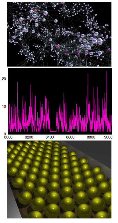
Figure 1: Illustration of three levels of the charge transport modeling. Bottom: Simulations of SET processes on nanoparticle array between the electrodes; Middle: Fractal analysis of the time series of the number of tunnelings per time unit in the assembly; Top: Algebraic topology analysis of the graph representing the phase-space manifold behind the sequence of events in the time series.

In particular: (i) We construct several two-dimensional assemblies of nanoparticles connected by tunneling junctions of a given structure. Then, setting the electrodes (cf. an example in Fig. 1 bottom) and slowly ramping the voltage bias, we simulate SET through such assemblies. (ii) We sample the time series of the relevant observables and perform the fractal analysis of these time series, as described in Methods, to determine the quantitative indicators of aggregate fluctuations. Here, we consider temporal fluctuations of the number of tunnelings per time unit, $N_{Q}(t_{k})$, an example is shown in Fig. 1 middle. (iii) Given recent developments of time-series–graphs duality stoch-visibility ; visibility ; we-PRE , we convert these time series into graphs. The sets of data points specify a manifold in the phase space of the system’s states that are involved in the course of events; the resulting graph then contains connections between these states. To explore the connection complexity among the system’s states, we use algebraic topology techniques (see Methods), and study higher order combinatorial spaces (simplexes) of these graphs. Our comparative analysis of different nanoparticle assemblies reveals a consistent correlation between the occurrence of collective charge transport, topological complexity of the phase space manifolds, and the $I(V)$ nonlinearity.

2 Theoretical Background and $I(V)$ Nonlinearity of Different Assemblies

The system of small metallic nanoparticles arranged on a substrate conducts when the applied bias exceeds a global threshold $V_{T}$, which is characteristic of the Coulomb blockade regime book-tn-97 ; CB-coopertunnelingExp-2008 ; we-review . In the Coulomb blockade conditions, the charging energy of a nanoparticle by a single electron $\Delta E_{s}=e^{2}/2C\gg k_{B}T$, where $C$ is the capacitance of the nanoparticle. The electrons, which are localised on nanoparticles, are transported by tunnelings through the junction between two nanoparticles when the voltage increases to exceed the Coulomb blockade voltage. The tunneling resistance satisfies the condition $R_{t}\gg h/e^{2}$ and the characteristic time scale is given by $\Delta t\sim R_{t}C$. The array of nanoparticles thus represents a capacitative coupled system, as described in the original work mw-ctasmd-93 . In we-review this theoretical concept is generalised to consider an arbitrary structure of the nanoparticle system, which is described by the adjacency matrix $A_{ij}$ of the underlying nanonetwork. In particular, the electrostatic energy $E$ of the assembly can be written in the matrix form as the follows

$$E=\frac{1}{2}\mathbf{Q}^{\dagger}\mathbf{M}^{-1}\mathbf{Q}+\mathbf{Q}\cdot\mathbf{V}^{ext}+Q_{\mu}\Phi^{\mu}\quad.$$ (2)

where summation over $\mu$ applies and the potential corresponding to the electrodes has the components

$$V^{ext}_{i}=\sum_{j,\mu}M_{ij}^{-1}C_{j,\mu}\Phi^{\mu}.$$ (3)

Here, $\mathbf{Q}$ represents the vector of charges and $\mathbf{\Phi}$ the potential of nanoparticles $i=1,2,\cdots N$. They satisfy the following relation at each nanoparticle:

$$Q_{i}=\sum_{j}C_{ij}(\Phi_{i}-\Phi_{j})+\sum_{\mu}C_{i,\mu}(\Phi_{i}-\Phi_{\mu})$$ (4)

where $C_{ij}=CA_{ij}$ represents the capacitance between neighbouring nanoparticles. The adjacency matrix element $A_{ij}=1$, when the particles $i\leftrightarrow j$ are within the tunneling distance while $A_{ij}=0$, when the distance between the particles is larger than the tunneling radius for the considered type of nanoparticles we-review ; zabet-review2008 . The index $\mu\in\{+,-,g\}$ stands for the positive and negative electrode and the gate, respectively. Thus, the elements of the capacitance matrix $\mathbf{M}$ depend on the structure of the assembly:

$$M_{ij}=\delta_{ij}\left(\sum_{j}C_{ij}+\sum_{\mu}C_{\mu,i}\right)-C_{ij}.$$ (5)

Then the potential at a nanoparticle $i$ can be expressed as

$$\Phi_{i}=\sum_{j}M_{ij}^{-1}Q_{j}+V_{i}^{ext}$$ (6)

in terms of all coupled charges and the potential at the electrodes.

The system is driven by slowly increasing the voltage bias between the electrodes. Thus, the tunnelings start between the high-voltage electrode and the first layer of nanoparticles, cf. Fig.1, and gradually pushing through the sample the front reaches the other electrode when $V\simeq V_{T}$. Then the current through the sample can be measured. Due to the long-range electrostatic interactions, every tunneling event affects the potential–charge relation (6) away from the event junction. Consequently, the energy change in the whole assembly occurs. Considering a particular tunneling event $a\to b$ from the nanoparticle $a$ to its neighbour nanoparticle $b$, the charge $Q_{i}$, measured in the number of electrons $e$, at a nanoparticle $i$ changes as

$$Q_{i}^{\prime}=Q_{i}+\delta_{ib}-\delta_{ia}\ ,$$ (7)

causing the energy change of the assembly $\Delta E_{a\to b}=E(\mathbf{Q^{\prime}})-E(\mathbf{Q})$. As discussed in detail in Ref. we-review , introducing the following quantity

$$V_{c}=\sum_{i}Q_{i}M_{ic}^{-1}\ ,$$ (8)

allows to write the energy change of the assembly due to the tunneling $a\to b$ in a concise form

$$\Delta E_{a\to b}=\frac{1}{2}\left(M_{aa}^{-1}+M_{bb}^{-1}-M_{ab}^{-1}-M_{ba}^{-1}\right)\;$$ (9)

$$+V_{b}-V_{a}+V_{b}^{ext}-V_{a}^{ext},$$ (10)

and similarly for tunnelings between the electrodes and a nanoparticle $a$

$$\Delta E_{a\leftrightarrow\pm}=\pm V_{a}+\frac{1}{2}M_{aa}^{-1}.$$ (11)

Theoretically, for a given value of the external voltage $V$, the tuneling rate $\Gamma_{a\to b}$ is determined by the energy change $\Delta E_{a\to b}$ according to the formula book-tn-97

$$\Gamma_{a\to b}=\frac{1}{eR_{a\to b}}\frac{\Delta E_{a\to b}/e}{1-\mathrm{e}^{-\Delta E_{a\to b}/k_{B}T}}\ .$$ (12)

Consequently, the current through the junction between the nanoparticles $a\leftrightarrow b$ is given by the balance of the tunnelings

$$I_{a\leftrightarrow b}(V)=e\left[\Gamma_{a\to b}(V)-\Gamma_{b\to a}(V)\right]\ .$$ (13)

The total current across the sample is thus given by the tunneling rates between the last layer of the nanoparticles and the low-voltage electrode. Note that the voltage drop through the sample according to (6) is nonlinear.

In the numerical implementation of the SET processes we-review ; MSBT_simulations2007 , the quantity $V_{c}$ defined by (8) is computed recursively

$$a\to b:V_{c}^{\prime}=V_{c}+M_{bc}^{-1}-M_{ac}^{-1}\ ,a\to\pm:V_{c}^{\prime}=V_{c}\pm M_{ac}^{-1}.$$ (14)

following every tuneling in the system. A more detailed description of the simulations is given in Methods.

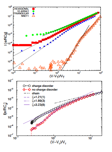
Figure 2: Current-Voltage curves for different nanoparticle assembles. Top: Curves from top to bottom correspond to one-dimensional chain, regular hexagonal and triangular arrays, and irregular structure NNET (cf. Fig. 4); Bottom: The nanonetwork SF22 (cf. Fig. 4) in the presence of charge disorder (upper curve) and without charge disorder (lower curve).

As mentioned in the Introduction, the nonlinearity exponent in I–V characteristics, Eq. (1), strongly depends on the structure of the nanoparticle assembly mw-ctasmd-93 ; rhc-sbcvcotdasmd-95 ; plj-etmna-01 ; we-NL2007 ; we-Oxford ; khondaker-PhysChemC2013 . Moreover, it was observed that in the same structure the exponent $\zeta$ changes with variations of the distance between the electrodes and their size we-Oxford ; CB-electrodes . Our simulations of SET in different nanoparticle assemblies we-NL2007 ; MSBT_simulations2007 ; we-review confirm these experimental findings. Fig. 2 shows $I(V)$ curves obtained in different nanonetworks including the structures studied in this work, cf. Fig. 4. For a single chain of nanoparticles, the current–voltage dependence is linear, i.e., $\zeta\simeq 1$, whereas for two-dimensional nanonetworks with a controlled structure $\zeta>2$, depending on the structure and the electrodes size. Specifically, within numerical error bars, we find $\zeta=2.30$ and $\zeta=3.0$ in a regular triangular and hexagonal arrays, respectively, with extended electrodes we-review , in a good agreement with the experimental results mw-ctasmd-93 ; plj-etmna-01 . An enhanced nonlinearity $\zeta=3.9$ characterises $I(V)$ curves in the highly irregular structure possessing a combination of compact areas and large voids (NNET in Fig. 4). The results agree well with the experimental studies of similar structures in we-NL2007 . The curve is also shown in the top panel of Fig. 2. The lower panel in Fig. 2 shows $I(V)$ dependence in the nanonetwork SF22. Its structure, also shown in Fig. 4, has a scale-free distribution of cells and a fixed branching. The simulations of SET in this nanonetwork yield $\zeta=3.23$ for a narrow voltage range. However, we obtain a reduced exponent $\zeta=1.89$ but an extended scaling region in the presence of charge disorder. In general, charge disorder originates from fractional charges on the substrate mw-ctasmd-93 ; plj-etmna-01 ; CB-1Dwd-granularmetalsTh2005 ), which causes a weaker nonlinearity. In the structure with nearly hexagonal cells, CNET in Fig. 4, the simulations performed in we-review using varied sizes of the electrodes resulted in a weakly reduced exponent $\zeta\in[2.3,2.5]$. A more recent study of regular arrays CB-electrodes suggests that $\zeta$ decreases as a logarithm of the ratio between the size of electrode and their distance.

3 Methods

The modeling approach on three levels mentioned in the Introduction encompasses different scales and algorithms, from the single-electron tunnelings at each junction of the nanonetwork in real space to collective charge fluctuations of the whole assembly, which are studied in time and the abstract phase space manifolds. The computational hierarchy is described as follows.
I. Simulations of SET on nanonetworks. The SET processes are simulated in four different nanoparticles assemblies represented by the nanonetworks in Fig. 4. First, the structure of the nanonetwork is included by specified adjacency matrix $\mathbf{A}$ and the electrodes are set to some periphery nodes. Usually, we chose $P/4$ nodes in the case of extended electrodes, or a single node, in the case of point-size electrodes, at two opposite sides of the network; here, $P$ is the number of periphery nodes of a given structure (see Fig. 1). Then the capacitance matrix and its inverse are computed and the vectors $\mathbf{Q}$ and $\mathbf{V_{+}}$ are initialized as zeros. To start the process, the time $t$ is initialised and the bias voltage set. For each value of the bias in the range $V\in[0,V_{max}]$ the number of steps are performed as follows. At each step, a tuneling is attempted along each junction $i\to j$ and the values $V_{c}$ for all nodes updated according to (14) and the corresponding energy charges $\Delta E_{i\to j}(t)$ are computed. Then, each tuneling rate $\Gamma_{i\to j}(t)$ is determined according to (12); the delay time $\Delta t_{ij}$ of the tuneling along the $i\to j$-junction is estimated. Following the description in we-review , $\Delta t_{ij}=\frac{-log(1-x_{ij})-\sum_{k>k_{0}}\delta t_{k}\Gamma_{i\to j}(t_{k})}{\Gamma_{i\to j}(t)}$, where $t_{k_{0}}$ is the time of the last tunneling at the junction and $x_{ij}$ is a uniform random number. The tunneling along the junction with a minimal delay time is processed and the time increased accordingly $t\to t+\Delta t_{ij}$. Subsequently, the charge $Q_{i}$ and $V_{i}$ are updated for all nodes, and the process is repeated to find next tunneling event and so on. The simulated data are in the limit $C/C_{g}=10^{-4}$, where a faster algorithm for computing the inverse of the capacitance matrix can be used we-review . We also keep $T=0$ and $\Phi_{-}=\Phi_{g}=0$ while $\Phi_{+}=V$, the applied voltage. The simulations are performed until $V\gtrsim 10V_{T}$ in the corresponding nanonetwork. To sample time series of interest for this work, we set an appropriate time unit according to the average tunneling rate $\delta t=a/\langle\Gamma_{ij}\rangle$ in each nanonetwork. The parameter $a=1$ in the one-dimensional array and takes different valueswe-review $a=$4.11 and 17.1 in CNET and NNET, respectively, in connection with the estimated number of potential paths in these irregular arrays. Then the time series represents the sequence of the number of tunnelings $N_{Q}(t_{k})$, $k=1,2\cdots$ in the entire array per the identified time unit.

II. Fractal time series analysis and temporal correlations. The occurrence of collective charge fluctuations manifests in long-range temporal correlations, clustering of events and fractal features of time series. Various indicators of the collective behavior are determined by analysis of the time series of the number of tunnelings $N_{Q}(t_{k})$. In particular, the temporal correlations occurring in the streams of events result in the power spectrum

$$S(\nu)\sim\nu^{-\phi}$$ (15)

with a power-law decay in a range of frequencies $\nu$. The avalanches of tunnelings accompany such temporal correlations. Using the standard numerical procedure tadic1999 ; we-SciRep2015 , the avalanches are identified in the stationary signal above $V_{T}$. The size of an avalanche comprises the area below a regular part of the signal above the zero thresholds. A broad distribution of avalanche sizes with a power-law tail suggests that, in a state with long-range correlations, the size of a triggered avalanche is not necessarily proportional to the triggering action. Moreover, the system’s relaxation in the response to the external driving is characterized by the differences between the size of consecutive events ( first return). The following expression, characteristic of the nonextensive statistical mechanics tsallis-2009_intro ; temporal-corr-AR2013 ; pavlos_q-returns2014 ,

$$P_{\kappa}(X)=A\left[1-(1-q_{\kappa})\left(\frac{X}{X_{0}}\right)^{\kappa}\right]^{-1/1-q_{\kappa}}$$ (16)

satisfactorily reproduces the distributions of the avalanche sizes, i.e., $q_{1}$-exponential, for $\kappa=1$, and the returns $q_{2}$-Gaussian, for $\kappa=2$.

According to the fractal analysis of complex signals MFRA-uspekhi2007 , the time series profile $Y(i)=\sum_{k=1}^{i}(N_{Q}(t_{k})-\langle N_{Q}(t_{k})\rangle$ is divided into $N_{n}$ segments of length $n$. The standard deviation $F_{2}(\mu,n)=\frac{\sum_{i=1}^{n}[Y((\mu-1)n+i)-y_{\mu}(i)]^{2}}{n}$ around the local trend $y_{\mu}(i)$ is computed at each segment $\mu=1,2,\cdots N_{n}$. Then the average over all segments exhibits a scaling law

$$F_{2}(n)=(1/N_{n})\sum_{\mu=1}^{N_{n}}F_{2}(\mu,n)\sim n^{H}$$ (17)

with respect to the varied segment length $n$, where $H$ is Hurst exponent. While $H=1/2$ characterises random fluctuations, the values $H\in(1/2,1)$ indicate the persisten fluctuations of the fractional Gaussian noise signal fractalSPP ; MFRA-uspekhi2007 ; dmfra-sunspot2006 .

III. Mapping time series onto QTS-graphs. The sequence of events captured by the time series of the number of tunnelings represents a manifold in the state space of the underlying nanonetwork. Dealing with a fractal signal (see Results), we expect a more complex connections among these states to exist beyond the actually realised sequence. To reveal such complexity of the system’s phase space, we use the mapping of time series to mathematical graphs recently developed visibility ; stoch-visibility . Here, we apply the ’natural visibility’ mapping visibility ; we-PRE , which is particularly suitable in the case of persistent fluctuations we-PRE . The mapping procedure is illustrated in Fig. 3. Each data point of the time series is represented by a node of the graph, here termed QTS-graph to indicate the charge fluctuations time series. The node is connected by undirected links with all other data points that are ’visible’ from that data point, where the vertical bars are considered as non-transparent. Note that by varying the mapping procedure different graphs can be obtained. However, here we use the same mapping procedure for different time series (i.e., charge fluctuations in different nanonetworks) and perform a comparative analysis of the structure of the resulting graphs. For this purpose, equal parts of the time series are mapped in each of the considered nanoparticle systems, i.e., 2000 data points, skipping the initial 8000 points.

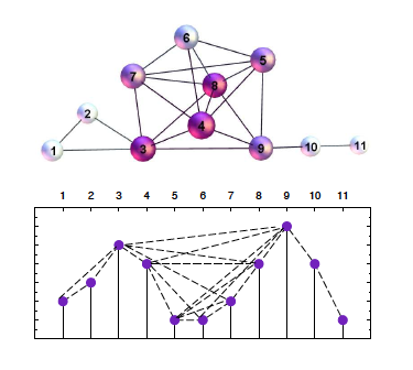
Figure 3: The sequence of data points in the lower pannel is mapped onto a graph in the upper pannel; each data point becomes a node of the graph, while the graph’s edges are inserted according to the ’natural visibility’ between data points, indicated by broken lines.

IV. Algebraic topology measures of QTS-graphs. Beyond standard graph theory measures bb-book ; sergey-lectures , the algebraic topology of graphs jj-book is utilised to determine the higher-order structures of a graph, i.e., simplicial objects and their collections, simplicial complexes, closed under the inclusion of faces. Using the paradigm of Taylor expansion, such combinatorial spaces correspond to higher-order terms while the graph itself represents the linear term. Recently, the computational topology techniques have been applied to analyse the hierarchical organisation in online social networks we-PhysA2015 , study of grain connectedness in trapped granular flow AT-granular , and to reveal the changes in the topological structure of state space across the traffic jamming regime we-PRE .

The method that we use Bron ; cliquecomplexes identifies simplexes as maximal complete subgraphs or cliques. Thus, $q=0$ represent an isolated node, $q=1$ two nodes connected with a link, $q=2$ is a triangle, $q=3$ a tetrahedron and so on until $\sigma_{q_{max}}$, which identifies the highest order clique present in the graph. Faces of a simplex $\sigma_{q}$ are the subsets $\sigma_{r}<\sigma_{q}$. The method determines cliques of all orders and identifies the nodes that belong to each clique. Utilising this rich information, we characterise the topological complexity of the graph at the global graph’s level, i.e., by defining various structure vectors, as well as the level of each node we-PhysA2015 ; we-PRE . In particular, having identified the graph’s topology layers $q=0,1,2,\cdots q_{max}$, we describe the number of cliques and how they are interconnected via shared faces at each level from $q_{max}-1,...,1$:

• Three structure vectors of graph have the components $G_{q}$, $n_{q}$ and ${\hat{G}_{q}}=1-G_{q}/n_{q}$, which determine, respectively, the number of connected components at the level $q$, the number of simplexes from the level $q$ upwards, and the degree of connectedness between the simplexes at $q$-level.

• The node’s structure vector is defined we-PhysA2015 by the components $G^{i}_{q}$, the number of simplexes of order $q$ to which the node $i$ participates. Then $dim(G_{i})=\sum_{q}G^{i}_{q}$ is the node’s topological dimension.

• The topological entropy $S_{G}(q)$ and the “response” function $f_{q}$ are defined we-PRE using the above quantities. Namely, the probability that a particular node $i$ contributes to the occupation of the topological level $q$ is $p^{i}_{q}=G^{i}_{q}/\sum_{i}G^{i}_{q}$. Then the graph’s entropy is

  $$S_{G}(q)=-\frac{\sum_{i}p_{q}^{i}log_{10}p_{q}^{i}}{log_{10}\sum_{i}(1-\delta_{G_{q}^{i},0})}\ ,$$ (18)

  where the sum in the denominator indicates the number of nodes with a nonzero entry at the considered topology level. The $q$-level component $f_{q}$ is defined as the number of simplexes and shared faces at the topology level $q$.

Notice that that the topological “response” $f_{q}$ is different from the component $n_{q}$ of the above defined second structure vector. The study in we-PRE have shown that the function $f_{q}$ precisely captures the topology shifts occurring in the underlying time series due to changed driving conditions.

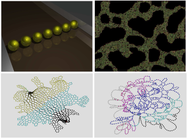
Figure 4: Top left: a 3-dimensional rendering of a chain of nanoparticles on a substrate and the attached electrodes. Top right: A 2-dimensional projection of the nanonetwork NNET with 5000 nanoparticles self-assembled by the evaporation methods (data are from Ref. we-NL2007 ). The lines indicate the tunneling junctions while a nanoparticle is found at the intersections. Bottom: CNET with a point-size electrodes (left) and SF22 with the extended electrodes (right), both grown by the cell aggregation we-iccs2006 . The voltage drop across the sample is indicated by the color of the network’s areas with high, intermediate and low potential.

4 Results and Discussion

4.1 Nanonetworks with different structural components and the origin of cooperative charge transport

For a comparative analysis of charge transport, the simulations of SET are performed in four nanoparticle assemblies with different structural characteristics. Specifically, two self-assembled nanoparticle arrays on a substrate, which are represented by the nanonetworks in the top row of Fig. 4, and two computer-generated structures, in the bottom row. For this work, these structures are identified as follows. The one-dimensional chain of nanoparticles between the electrodes, where we assume the presence of charge disorder $x_{i}\in[0,1]$ as a uniform random number, is named 1Dwd. Further, NNET is a strongly inhomogeneous structure of nanoparticles, which is self-assembled on the substrate by the evaporation process we-NL2007 . The occurrence of empty areas of different sizes as well as the regions where the nanoparticles appear to be densely packed is the marked characteristics of this assembly. CNET, shown in the lower left, and SF22 in the lower right panel, are grown by the cell aggregation process we-iccs2006 . In these networks, we control the appearance of two relevant structural elements—branching and the extended linear segments—that appear statistically in the above described self-assembled structures. Namely, CNET has nearly regular hexagonal cells, resembling the dominant shapes in the dense areas of the NNET, while SF22 exhibits voids of different sizes; the cell sizes are taken from a power-law distribution with the exponent 2.2 we-SFloops2006 . Moreover, both CNET and SF22 have a fixed degree of internal nodes $k=3$, which reduces the branching possibilities for the tunnelings, in contrast with the NNET, where a broader degree distribution of nodes is found we-NL2007 ; we-review . Furthermore, the electrodes are set to the left and right edge of the NNET, thus touching the closest layer of the nanoparticles. Similarly, the extended positive and negative electrode are set each along a quarter of the periphery nodes, indicated by white and black nodes in SF22 structure in Fig. 4. In contrast, the point-size electrodes are attached to two periphery nodes in CNET and two nanoparticles at the opposite ends of the 1Dwd chain.

The situation with point-size electrodes in CNET in Fig. 4 readily illustrates the importance of local structure for the collective charge transport of the assembly. Increasing voltage bias permits tunnelings between the electrode and the first layer, consisting of two connected nanoparticles. Then further tunnelings can occur by breaking the Coulomb blockade along the junctions towards nearest neighbor nanoparticles. The preferred direction of tunnelings follows the potential drop, which is indicated by the different color of nodes. Apart from the long-range electrostatic interactions, the local balance between the charge and potential (6) at each nanoparticle depends on its neighbourhood. At $V\sim V_{T}$ the number of charges in the system is large enough to allow the first conduction channel to form along the shortest path between the electrodes. For $V\gtrsim V_{T}$ the conditions for the appearance of another next-to-shortest path are met. Here, the branching possibilities for the charge flow play an important role. Consequently, the process can involve several paths thus making a river-like structure that drains at the last layer of nanoparticles. These paths often share some central nodes and junctions. The most used junctions (indicated by thick lines of CNET in Fig. 4) make the main conduction channels we-review , whose geometry crucially depends on the local structure. Draining along the conduction paths can cause a cascade of tunnelings, where each event satisfies the local Coulomb blockade threshold and charge–potential balance. Thus, in this range of voltages, the SET represents a dynamical percolation problem plerj-ptnrt-04 where several conduction paths contribute to the measured current, resulting in the nonlinear $I(V)$ curves in Fig. 2. The quantitative analysis presented in the remaining part of this section confirms this picture. On the other hand, for $V\gg V_{T}$, the local potential exceeds the Coulomb blockade potential yielding Ohmic conduction and the crossover to a linear $I(V)$ dependence in Fig. 2.

4.2 Temporal correlations and the evidence of collective charge fluctuations

The number of tunnelings per the identified unit interval is recorded from the SET simulations in four nanonetworks of Fig. 4. The resulting time series are shown in Fig. 5. The corresponding power spectra displayed in top panel of Fig. 5, indicate the occurrence of temporal correlations that depend on the structure of the underlying nanonetwork. Specifically, the Eq. (15) applies within a different range of frequencies and different exponent $\phi$, which is shown in the legend. Apart from slight variations in the exponent, the power spectrum reveals the certain similarity between the charge fluctuations in the nanonetworks SF22 and 1Dwd, on one side, and NNET and CNET, on the other. Hence, the dominance of the linear elements, which is obvious to the chain structure, seems to play a role in the SF22 too. The spectrum exhibits the power-law decay (15) in the entire range of $\nu$. On the other hand, plenty of branching possibilities in CNET and NNET lead to the occurrence of multiple paths; a typical scale appears, which leads to the peak in the spectrum between the correlated high-frequency part and the rest of the spectrum resembling a white noise.

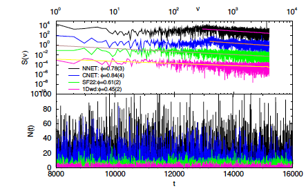
Figure 5: Time series of the number of tunnelings (bottom panel) and the corresponding power spectrum (top panel) in four nanoparticle networks from Fig. 4. The legend and color apply to both panels. The signal for NNET is scaled by 1/5 to fit the scale.

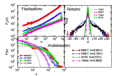
Figure 6: For four nanonetworks from Fig. 4: Double logarithmic plot of the fluctuations $F_{2}(n)$ against the segment size $n$, top left, and the scaling regions indicated by a straight line on each curve; The distributions $P(s)$ of the avalanche sizes $s$, bottom left, and the distribution $P(d)$ of the first returns $d$ of the signal.

A further similarity between these two groups of nanostructures is found considering the nature of fluctuations and the statistics of avalanches, which are displayed in Fig. 6. Computing the standard deviations around a local trend on the segment of length $n$ of the time series, we find the scaling regions according to Eq. (17) and determine the corresponding Hurst exponent. The values of the exponents for all time series, which are listed in the legend, suggest that persistent fluctuations of charge transport occur in all considered nanonetworks. The fluctuations in the linear chain of nanoparticles and the SF22 structure have a similar value of the Hurst exponent, again suggesting the relevance of the extended linear segments in these nanonetworks. Notably, the values of $H$ for these nanostructures are slightly larger than the case of the randomized time series, where $H=0.5$ within error bars. However, the two structures CNET and NNET, which allow the formation of more communicating paths, exhibit much stronger fluctuations and consequently larger values of the Hurst exponent. Furthermore, the statistics of the returns $d\equiv N_{Q}(t_{k})-N_{Q}(t_{k-1})$ and the sizes $s$ of clustered events (avalanches) also suggests a similar grouping of these nanostructures. On one side, the charge fluctuations in SF22 and 1Dwd structures has the exponential distribution of avalanche sizes (with a larger cut-off in the case of SF22) and Gaussian distributions of the returns. On the other hand, non-Gaussian fluctuations are found in the case of CNET and NNET. In this case, the distribution of avalanche sizes exhibits a power-law tail compatible with the expressions (16) with $\kappa=1$ and $q_{1}\sim 1.33$. Similarly, the tails of the distribution of the returns can be fitted with (16), where $\kappa=2$, i.e., $q_{2}$-Gaussian, which is often found in complex signals pavlos_q-returns2014 . It should be stressed that the part of the data for small returns and small avalanches in these two nanonetworks virtually coincides with the ones found in the chain and SF22 structures. These weak fluctuations correspond to sporadic tunnelings away from the main conduction paths. This feature of the fluctuations is particularly pronounced in the case of CNET, where the most used area of the nanonetwork is reduced due to the point-size electrodes (cf. Fig. 4).

4.3 Topology of phase space manifolds related with the collective charge fluctuations

The time series of charge fluctuations $N_{Q}(t_{k})$ are converted into QTS-graphs, as described in Section 3. With analysis of these graphs, we provide a robust topological description of the collective charge fluctuations in different nanoparticle assemblies. For a better comparison, we map an equal segment of each time series in the considered nanoparticle assemblies. Hence, we generate four QTS-graphs of 2000 nodes; each QTS-graph clearly relates with the underlying nanoparticle structure in Fig. 4, from which the time series is taken. The utilized mapping rules account for the strength of fluctuations; consequently, the QTS-graphs of different structure are obtained. Fig. 7 displays the adjacency matrices of all four QTS-graphs.

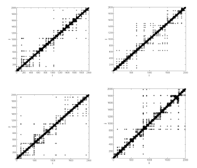
Figure 7: Adjacency matrix of the QTS-graph related with the charge fluctuations in the nanoparticle assemblies (a) 1Dwd, (b) NNET, (c) CNET and (d) SF22.

The pronounced block-diagonal structure in the adjacency matrices for QTS-graphs of CNET and 1Dwd indicates the occurrence of communities of dense links. While in the case of QTS-graphs of NNET and SF22, a sparse structure of connections among the diagonal blocks appears, which is compatible with a hierarchical organization of communities identifiable at the graph level. The ranking distributions of the node’s degree and topological dimension of all QTS-graphs are shown in Fig. 8. Separate fits for small and large rank according to the discrete generalized beta function are provided, except for the case of FS22, where a satisfactory fit is obtained by a power-law decay with a cut-off (see legends).

Table 1: Standard graph theory measures ($d$–diameter, $\langle k\rangle$–average degree, $\langle\ell\rangle$–average path length, Cc–clustering coefficient, the number of triangles, modularity) of the QTS-graphs representing collective charge fluctuations in nanonetworks from Fig. 4.

QTS-graph	$d$	$\langle k\rangle$	$\langle\ell\rangle$	Cc	No.triang	modul
-1Dwd	10	6.98	5.14	0.77	10314	0.907
-SF22	10	7.27	4.89	0.76	10987	0.897
-CNET	9	8.91	4.66	0.81	17369	0.906
-NNET	11	8.35	4.86	0.79	15418	0.909

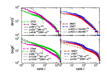
Figure 8: Ranking distributions of the node’s degree (lower panels) and topological dimension (upper panels) in the studied QTS graphs of charge fluctuations in four nanonetworks from Fig. 4.

A collection of standard graph-theoretic measures of all QTS-graphs is given in Table 1, exhibiting small differences at the graph level. However, the higher-order structures of these graphs, which are described by the algebraic topology measures, can be considerably different; the results are displayed in Figs. 9-10 and illustrated by Fig. 11.

The higher-order structures of the QTS-graphs are revealed by determining the components of three structure vectors, which are defined in section 3. The results are displayed in Fig. 9. Their numerical values are summarized in Table 2. For a comparison, we also show the results for a graph, which is obtained from a randomized time series; for this purpose, such series is obtained by interchanging randomly-selected pairs of data points in the time series from NNET.

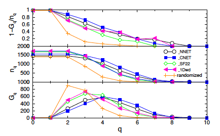
Figure 9: Components of the 1st, 2nd and 3rd structure vector, $G_{q}=1-G_{q}/n_{q}$, $n_{q}$ and ${\hat{G}_{q}}$, respectively, plotted against the topology level $q$ in the QTS-graphs related with the time series of charge fluctuations in the underlying nanoparticle structures, which are indicated in the legend, and a randomized time series.

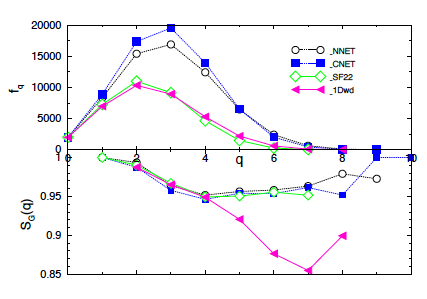
Figure 10: The entropy $S_{Q}(q)$ and the number of simplexes and shared faces $f_{q}$ at the topological level $q$ of the QTS graphs of the charge fluctuations in the indicated nanoparticle assemblies.

Notably, the randomized time series results in a graph exhibiting much simpler structure than the other graphs, which represent the fractal time series. The topological complexity of these QTS-graphs manifests in the occurrence of a vast number of topological levels $q=0,1,2\cdots q_{max}$ in accord with the number of combinatorial spaces and their interconnections at higher topological levels. As an example, in Fig. 11 we display the QTS-graph of NNET assembly. In two separate plots we also demonstrate the complexity of its top topological levels, $q=8$ and $q=9$. Specifically, it contains eight 10-cliques; three 10-cliques are separated, and the other five are interconnected via 9-cliques at the lower level $q=8$. Here, according to the table 2, 36-8=28 additional 9-cliques exist and are interconnected such that 33 components occur at the level $q=8$. That is, 33-28=5 components are identifiable at the upper level, cf. Fig. 11 bottom left. Considering the level below, $q=7$, gives 105-36=69 new 8-cliques and

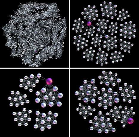
Figure 11: The structure of connections of the phase space manifolds corresponding to the charge fluctuations in the nanoparticle network NNET: complete QTS_-NNET graph (top left) and its highest topological layers $q=8$, top right, and $q=9$, bottom left. For comparison, the layer $q=8$ of the QTS_-CNET graph is displayed, bottom right. In figures of the higher topological layers, ID of each node refers to the index of the time interval $t_{k}$ of the time series. All edges between these nodes that exist in the adjacency matrix are shown.

86 components, which suggests that maximally 86-69=17 groups of nodes can be distinguished at the level $q=8$. Among these, five groups contain higher cliques, leaving at most 12 groups that are visually distinct in the top right figure 11. In contrast, the single 11-clique in QTS-graph of CNET remains isolated down to the level $q=7$ (cf. table 2). Together with 17 other 9-cliques that appear at the level $q=8$, they make 18 components. At the level below, we identify 137-18 =119 new 8-cliques. Then comparing the number of components, 128-119=9 suggests that the cliques at the upper level $q=8$ make at most nine groups, one of which refer to the 11-clique of the top levels. This structure is also shown in Fig. 11 bottom right.

According to Fig. 9, the second structure vectors of QTS-graphs of SF22 and 1Dwd exhibit certain similarity. Interestingly enough, the presence of charge disorder in the linear chain of nanoparticles leads to a more complex QTS-graph than the SF22 assembly. Namely, the charge disorder blocks the only existing path in the linear chain, which results in a sequence of zero entries in the time series, which is mapped onto a large clique linked to two or more near non-zero entries. In contrast, blocking a linear segment in SF22 structure causes tunnelings along the alternative paths. Hence, no abrupt changes in the time series occur. Apart from the high topology levels, the similarity between the QTS-graphs of NNET and CNET, on one side, and SF22 and 1Dwd, on the other, is apparent at lower $q$-levels, cf. Fig. 9. These findings also apply to the topological response function $f_{q}$ and the entropy $S_{Q}(q)$, shown in Fig. 10. The occurrence of mutually isolated cliques, i.e, at $q=1$ or $q=q_{max}$, leads to the occupation probability $p_{q}^{i}\lesssim 1$ and the entropy close to zero. The simplicial complexes that occur at the intermediate $q$-levels share the faces at the level $q-1$. Hence, same nodes participate in the identified complexes, leading to a lower occupation probability of the level and the entropy drops, as shown in Fig. 10. The 2-dimensional nanoparticle assemblies exhibit complex QTS-graphs in which a large number of simplicial complexes, sharing many nodes, is observed. In contrast, a small number of such compounds occur in the case of the linear chain structure with charge disorder. Thus, a reduced number of nodes are involved; this situation manifests in a more pronounced entropy minimum at $q_{max}-1$ than in the other graphs.

5 Conclusions

Using the extensive numerical study at different scales, we have demonstrated how the structure of tunneling junctions in the arrays of metallic nanoparticles affects the collective nature of the charge transport within the Coulomb-blockade regime. The simulations of single-electron tunnelings in nanoparticle arrays of different architecture are combined with the fractal analysis of time series and algebraic topology techniques applied to the abstract graphs in the state space. We quantitatively describe the aggregate fluctuations at the global scale; the collective dynamics builds on communication among local events, which is enabled by the structural features of the nanoparticle network with junctions. Two structural components can locally affect the formation of the conducting paths between the electrodes encasing the array. These are the branching at each nanoparticle, which increases geometrical entanglement of the conduction paths, and the presence of linear segments whose tunneling conduction is better understood, which reduces it.

The comparative analysis of different nanonetworks in conjunction with the size of electrodes leads to the following general conclusions.

• A higher level of cooperation in the charge fluctuations through the sample that is measured by the fractal indicators of the time series is consistent with a larger topological complexity of the phase space manifolds yielding an enhanced $I(V)$ nonlinearity beyond the voltage threshold.

• A suitable combination of the local branching and global topological defects that allow a formation of large draining basins, as illustrated by NNET structure in our analysis, enables an enhanced collective dynamics.

• The size of electrodes can considerably influence the strength of aggregate fluctuations, and thus the structure of the complex phase space and the $I(V)$ curve. In particular, point-size electrodes enhance the formation of several nearly-shortest paths; they can be physically close to each other in arrays of a compact structure with an extensive branching along the main path. A good example is CNET studied in this work. On the other hand, the presence of significant linear segments, such as SF22, increases the difference between the path lengths, which reduces the probability of a coordinated drainage. In such cases, extended electrodes allow the formation of several channels of a similar structure.

Our analysis also sheds a new light onto the effects of the charge disorder on the system’s conduction capabilities. Both the temporal correlations and the topology of phase space manifolds demonstrate dramatic effects of charge disorder in the linear chain of nanoparticles, which comprises a single conduction path. In a two-dimensional array, such as SF22, blocking some linear segments of the structure by charge disorder affects the morphology of conduction basins, resulting in a reduced current.

The presented results reveal how the architecture implicates the emergent conduction features of nanoparticle assemblies. They may serve as a guide for the design of the nanoparticle devices with improved conduction. We have not explicitly considered the effects of finite temperature and varied widths of the tunneling junctions, which often appear in the experiments. They also may alter the tunneling process at the local scale and, according to this work, imply changes in the collective charge fluctuations. Apart from these practical aspects, our work stresses the importance of different modeling approaches. In this context, the methods of algebraic topology applied to the graphs in the system’s phase space are opening a new perspective for the analysis of fluctuations at a nanoscale.

Table 2: Components of three structure vectors of the graphs representing charge-fluctuation time series in nanonetworks from Fig. 4.

QTS-	-NNET			-CNET			-SF22			-1Dwd			-randomised TS
q	$G_{q}$	$n_{q}$	$\hat{G}_{q}$	$G_{q}$	$n_{q}$	$\hat{G}_{q}$	$G_{q}$	$n_{q}$	$\hat{G}_{q}$	$G_{q}$	$n_{q}$	$\hat{G}_{q}$	$G_{q}$	$n_{q}$	$\hat{G}_{q}$
0	1	1458	0.99	1	1550	0.99	1	1684	0.99	1	1721	0.99	1	1403	0.99
1	10	1458	0.99	6	1550	0.99	7	1684	0.99	7	1721	0.99	13	1403	0.99
2	265	1457	0.82	193	1549	0.88	455	1683	0.73	503	1721	0.71	904	1400	0.35
3	497	1326	0.63	399	1473	0.73	673	1410	0.52	733	1448	0.49	766	873	0.12
4	570	1025	0.44	594	1238	0..52	638	935	0.31	517	893	0.42	265	283	0.06
5	430	628	0.32	512	826	0.38	346	418	0.17	268	433	0.38	67	69	0.03
6	252	313	0.20	351	438	0.20	103	119	0.13	145	179	0.19	12	12	0
7	86	105	0.18	128	137	0.07	25	25	0	29	37	0.22	1	1	0
8	33	36	0.08	18	18	0				9	9	0
9	8	8	0	1	1	0
10				1	1	0

References

- (1) I. Kotsireas, R.V.N. Melnik, and B. West, editors. Advances in Mathematical and Computational Methods: Addressing Modern Challenges of Science, Technology and Society. American Institute of Physics, Vol. 1368, 2011.
- (2) P. Moriarty. Nanostructured materials. Reports on Progress in Physics, 64:297–381, 2001.
- (3) J. Liao, S. Block, S.J. van der Molen, S. Diefenbach, A.W. Holleitner, C. Schönenberg, A. Vladyka, and M. Calame. Ordered nanoparticle arrays interconnected by molecular linkers: electronic and optoelectronic properties. Chem. Soc. Review, 44:999–1014, 2015.
- (4) J. Živković and B. Tadić. Nanonetworks: The graph theory framework for modeling nanoscale systems. Nanoscale Systems MMTA, 2:30–48, 2013.
- (5) D. K. Ferry and S. M. Goodnick. Transport in Nanostructures. Cambridge University Press, 1997.
- (6) I.S. Beloborodov, A.V. Lopatin, V.M. Vinokur, and K.B. Efetov. Granular electronic systems. Rev. Mod. Phys., 79:469, 2007.
- (7) M. Šuvakov and B. Tadić. Modeling collective charge transport in nanoparticle assemblies. J. Phys. Condens. Matt., 22, 2010.
- (8) H. Fan, K. Yang, D.M. Boye, T. Sigmon, K.J. Malloy, H. Xu, G.P Lopez, and C.J. Brinker. Self-assembly of ordered, robust, three-dimesionalgold nanocrystal/silica arrays. Science, 304:567, 2004.
- (9) M. O. Blunt, M. Šuvakov, F. Pulizzi, C. P. Martin, E. Pauliac-Vaujour, A. Stannard, A.W. Rushforth, B. Tadić, P. Moriarty. Charge transport in cellular nanoparticle networks: meandering through nanoscale mazes. Nano Letter, 7(4):855, 2007.
- (10) M.O. Blunt, A. Stannard, E. Pauliac-Vaujour, C.P. Martin, Ioan Vancea, M. Šuvakov, U. Thiele, B. Tadić, and P. Moriarty. Patterns and pathways in nanoparticle self-organization. Oxford Univ. Press, Oxford, UK, 2010.
- (11) D. Joung, L. Zhai, and S.I. Khondaker. Coulomb blockade and hopping conduction in graphene quantum dots. Phys. Rev. B, 83, 2011.
- (12) D. Joung and S.I. Khondaker. Structural evolution of reduced graphene oxyde of varying carbon frcations investigated via Coulomb blockade transport. J. Phys. Chem. C, 117:26776-26782, 2013.
- (13) K.P. Loh, Q. Bao, and M. Chhowalla. Graphene oxide as a chemically tunable platform for optical applications. Nat. Chemistry, 2:1015-1024, 2010.
- (14) H. Kohno and S. Takeda. Non-Gaussian fluctuations in the charge transport of Si nanonchains. Nanotechnology, 18:395706, 2007.
- (15) I.S. Beloborodov, A.V. Lopatin, and V.M. Vinokur. Coulomb effects and hopping transport in granular metals. Phys. Rev. B., 72:125121, 2005.
- (16) T.B. Tran, I.S. Beloborodov, X.M. Lin, T.P Bigioni, V.M. Vinokur, and H.M. Jaeger. Multiple cotunneling in large quantum dot arrays. Phys. Rev. Lett., 95:076806, 2005.
- (17) W.A. Schoonveld, J. Wildeman, D. Fichou, P.A. Bobbert, B.J. van Wees, and T.M. Klapwijk. Coulomb-blockade transport in single-crystal organic thin film transistors. Nature, 404:977–980, 2000.
- (18) J. Kane, M. Inan, and R.F. Saraf. Self-assembled nanoparticle necklaces network showing single-electron switching at room temperature and biogating current by living microorganisms. ACS Nano, 4:317–323, 2010.
- (19) A. A. Middleton and N. S. Wingreen. Collective transport in arrays of small metallic dots. Phys. Rev. Lett., 71(19):3198–3201, 1993.
- (20) A. J. Rimberg, T. R. Ho, and J. Clarke. Scaling behavior in the current-voltage characteristic of one- and two-dimensional arrays of small metallic islands. Phys. Rev. Lett., 74(23):4714–4717, 1995.
- (21) M. N. Wybourne, L. Clarke, M. Yan, S. X. Cai, L. O. Brown, J. Hutchison, and J. F. W. Keana. Coulomb-blockade dominated transport in patterned gold-cluster structures. Jpn. J. Appl. Phys., 36:7796–7800, 1997.
- (22) R. Parthasarathy, X. Lin, and H. M. Jaeger. Electronic transport in metal nanocrystal arrays: The effect of structural disorder on scaling behavior. Phys. Rev. Lett., 87(18):186807, 2001.
- (23) R. Parthasarathy, X. Lin, K. Elteto, T. F. Rosenbaum, and H. M. Jaeger. Percolating through networks of random thresholds: Finite temperature electron tunneling in metal nanocrystal arrays. Phys. Rev. Lett., 92(7):076801, 2004.
- (24) T.S. Basu, S. Ghosh, S. Gierolta ka, and M. Ray. Collective charge transport in semiconductor-metal hybrid nanocomposites. Appl. Phys. Lett., 102, 053107, 2013.
- (25) Ch. George, I. Szleifer, and M. Ratner. Multiple-time-scale motion in molecularly linked nanoparticle arrays. ACS NANO, 7:108–116, 2013.
- (26) T.B. Tran, I.S. Beloborodov, J. Hu, X.M. Lin, T.F. Rosenbaum, and H.M. Jaeger. Sequential tunneling and inelastic cotunneling in nanoparticle arrays. Phys. Rev. B., 78:075437, 2008.
- (27) A. Zabet-Khosousi and A-A. Dihrani. Charge transport in nanoparticle assemblies. Chem. Rev., 108:4072–4124, 2008.
- (28) J.K.Y. Ong, Ch. Van Nguyen, S. Sayood, and R.F. Saraf. Imaging electroluminescence from individual nanoparticles in an array exhibiting room temperature single electron effect. ACS NANO, 7:7403–7410, 2013.
- (29) M. Šuvakov and B. Tadić. Topology of cell-aggregated planar graphs. In V. Alexandrov et al., editor, Computational Science — ICCS 2006, volume 3993 of Lecture Notes in Computer Science, pages 1098–1105, Berlin, 2006. Springer.
- (30) M. Šuvakov and B. Tadić. Simulation of the electron tunneling paths in network of nano-particle films. In Y. Shi et al., editor, Lecture Notes in Computational Science - ICCS 2007, volume 4488 of Lecture Notes in Computer Science, pages 641–648, Berlin, 2007. Springer.
- (31) B. Luque, L. Lacasa, F. Ballesteros, and A. Robledo. Feigenbaum graphs: A complex network perspective of chaos. PLOS One, 6, e22411, 2011.
- (32) F. Ballesteros, F. Luque, L. Lacasa, B. Luque, and J. C. Nuno. From time series to complex networks: the visibility graphs. Proc. Natl. Acad. Sci. USA, 105:4972, 2008.
- (33) M. Andjelković, N. Gupte, and B. Tadić. Hidden geometry of traffic jamming. Phys. Rev. E, 91:052817, 2015.
- (34) T. Narumi, M. Suzuki, Y. Hidaka, and S. Kai. Size dependence of current–voltage properties in Coulomb blockade networks. J. Phys. Soc. Japan, 80:114704, 2011.
- (35) B. Tadić. Dynamic criticality in driven disordered systems: role of depinning and driving rate in Barkhausen noise. Physica A: Statistical and Theoretical Physics, 270:125, 1999.
- (36) M. Mitrović Dankulov, R. Melnik, and B. Tadić. The dynamics of meaningful social interactions and the emergence of collective knowledge. Scientific Reports, 5:12197, 2015.
- (37) C. Tsallis. Introduction to nonextensive statistical mechanics : approaching a complex world. Springer, N.Y., 2009.
- (38) A. Pluchino, A. Rapisarda, and C. Tsallis. Noise, synchrony, and correlations at the edge of chaos. Phys. Rev. E, 87:022910, 2013.
- (39) G.P. Pavlos, L.P. Karakatsanis, M.N. Xenakis, E.G. Pavlos, A.C. Iliopoulos, and D.V. Sarafopoulos. Universality of non-extensive Tsallis statistics and time series analysis: Theory and applications. Physica A: Statistical Mechanics and its Applications, 395:58 – 95, 2014.
- (40) A.N. Pavlov and V. S. Anishchenko. Multifractal analysis of complex signals. Physics–Uspekhi, 50:819–834, 2007.
- (41) S.B. Lowen and M.C. Teich. Estimation and simulation of fractal stochastic point processes. Fractals, 3:183–210, 1995.
- (42) M. Sadegh Movahed, G. R. Jafari, F. Ghasemi, S. Rahvar, and M. R. Rahimi Tabar. Multifractal detrended fluctuation analysis of sunspot time series. Journal of Statistical Mechanics: Theory and Experiment, 2006(02):P02003, 2006.
- (43) B. Bollobas. Modern Graph Theory. Springer, New York, 1998.
- (44) S. Dorogovtsev. Lectures on Complex Networks. Oxford University Press, Inc., New York, 2010.
- (45) J. Jonsson. Simplicial Complexes of Graphs. Lecture Notes in Mathematics, Springer-Verlag, Berlin, 2008.
- (46) M. Andjelković, B. Tadić, S. Maletić, and M. Rajković. Hierarchical sequencing of online social graphs. Physica A: Statistical Mechanics and its Applications, 436:582 – 595, 2015.
- (47) I. Kondić, A. Goullet, C.S. O’Hern, M. Kramar, K. Mishaikow, and R.P. Behringer. Topology of force networks in compressed granular media. Eur. Phys. Lett., 97:54001, 2012.
- (48) C. Bron and J. Kerbosch. Finding all cliques of an undirected graph. Comm. ACM, 16:575-577, 1973.
- (49) H.-J. Bandelt and V. Chepoi. Metric graph theory and geometry: a survey, in Goodman, J. E.; Pach, J.; Pollack, R., eds. "Surveys on discrete and computational geometry: Twenty years later". Contemporary Mathematics, 453:49–86, 2008.
- (50) M. Šuvakov and B. Tadić. Transport processes on homogeneous planar graphs with scale-free loops. Physica A: Statistical Mechanics and its Applications, 372:354–361, 2006.