Efficient numerical methods for the random-field Ising model:
Finite-size scaling, reweighting extrapolation, and computation of response functions

Abstract

It was recently shown [Phys. Rev. Lett. 110, 227201 (2013)] that the critical behavior of the random-field Ising model in three dimensions is ruled by a single universality class. This conclusion was reached only after a proper taming of the large scaling corrections of the model by applying a combined approach of various techniques, coming from the zero- and positive-temperature toolboxes of statistical physics. In the present contribution we provide a detailed description of this combined scheme, explaining in detail the zero-temperature numerical scheme and developing the generalized fluctuation-dissipation formula that allowed us to compute connected and disconnected correlation functions of the model. We discuss the error evolution of our method and we illustrate the infinite limit-size extrapolation of several observables within phenomenological renormalization. We present an extension of the quotients method that allows us to obtain estimates of the critical exponent $\alpha$ of the specific heat of the model via the scaling of the bond energy and we discuss the self-averaging properties of the system and the algorithmic aspects of the maximum-flow algorithm used.

I Introduction

The random-field Ising model (RFIM) is one of the archetypal disordered systems Imry and Ma (1975); Aharony et al. (1976); Young (1977); Fishman and Aharony (1979); Parisi (1979); Cardy (1984); Imbrie (1984); Schwartz and Soffer (1985); Gofman et al. (1993); Esser et al. (1997); Barber and Belanger (2001), extensively studied due to its theoretical interest, as well as its close connection to experiments in condensed matter physics Belanger and Young (1991); Rieger (1995a); Nattermann (1998); Belanger (1998); Belanger et al. (1983); Vink et al. (2006). In particular, several important systems can be studied through the RFIM: diluted antiferromagnets in a field Belanger (1998), colloid-polymer mixtures Vink et al. (2006); Annunziata and Pelissetto (2012), colossal magnetoresistance oxides Dagotto (2005); Burgy et al. (2001), phase-coexistence in the presence of quenched disorder Cardy and Jacobsen (1997); Fernández et al. (2008); Fernandez et al. (2012), non-equilibrium phenomena such as the Barkhausen noise in magnetic hysteresis Sethna et al. (1993); Perković et al. (1999) or the design of switchable magnetic domains Silevitch et al. (2010), etc.

The existence of an ordered ferromagnetic phase for the RFIM, at low temperature and weak disorder, followed from the seminal discussion of Imry and Ma Imry and Ma (1975), when the space dimension is greater than two ($D>2$) Villain (1984); Bray and Moore (1985a); Fisher (1986); Berker and McKay (1986); Bricmont and Kupiainen (1987). This has provided us with a general qualitative agreement on the sketch of the phase boundary, separating the ordered ferromagnetic phase from the high-temperature paramagnetic one. The phase-diagram line separates the two phases of the model and intersects the randomness axis at the critical value of the disorder strength. Such qualitative sketching has been commonly used in most papers for the RFIM Newman et al. (1993); Machta et al. (2000); Newman and Barkema (1996); Itakura (2001); Fytas and Malakis (2008); Aharony (1978) and closed form quantitative expressions are also known from the early mean-field calculations Aharony (1978). However, it is generally true that the quantitative aspects of phase diagrams produced by mean-field treatments are very poor approximations.

On the theoretical side, a scaling picture is available Villain (1984); Bray and Moore (1985a); Fisher (1986). The paramagnetic-ferromagnetic phase transition is ruled by a fixed point [in the Renormalization-Group (RG) sense] at temperature $T=0$ Nattermann (1998). The spatial dimension $D$ is replaced by $D-\theta$, in hyperscaling relations ($\theta\approx D/2$). Nevertheless, one expects only two independent exponents Aharony et al. (1976); Schwartz and Soffer (1985); Gofman et al. (1993); Nattermann (1998), as in standard phase transitions Amit and Martin-Mayor (2005). Unfortunately, establishing the scaling picture is far from trivial. Perturbation theory predicts that, in $D=3$, the ferromagnetic phase disappears upon applying the tiniest random field Young (1977). Even if the statement holds at all orders in perturbation theory Parisi (1979), the ferromagnetic phase is stable in $D=3$ Bricmont and Kupiainen (1987). Non-perturbative phenomena are obviously at play Parisi (1994); Parisi and Sourlas (2002). Indeed, it has been suggested that the scaling picture breaks down because of spontaneous supersymmetry breaking, implying that more than two critical exponents are needed to describe the phase transition Tissier and Tarjus (2011).

On the experimental side, a particularly well researched realization of the RFIM is the diluted antiferromagnet in an applied magnetic field Belanger (1998). Yet, there are inconsistencies in the determination of critical exponents. In neutron scattering, different parameterizations of the scattering line-shape yield mutually incompatible estimates of the thermal critical exponent, namely $\nu=0.87(7)$ Slanič et al. (1999) and $\nu=1.20(5)$ Ye et al. (2004). Moreover, the anomalous dimension $\eta=0.16(6)$ Slanič et al. (1999) violates hyperscaling bounds, at least if one believes experimental claims of a divergent specific heat Belanger et al. (1983); Slanič and Belanger (1998). Clearly, a reliable parametrization of the line-shape would be welcome. This program has been carried out for simpler, better understood problems Martín-Mayor et al. (2002). Unfortunately, it is a common belief that we do not have such a strong command over the RFIM universality class.

The model has been also investigated by means of numerical simulations Rieger (1993); Nowak et al. (1998); Newman and Barkema (1996). However, typical Monte Carlo schemes get trapped into local minima with escape time exponential in $\xi^{\theta}$, where $\xi$ denotes the correlation length. Although sophisticated improvements have appeared Fernandez et al. (2011); Fytas et al. (2008); Vink et al. (2010); Ahrens et al. (2013); Picco and Sourlas (2015), these simulations produced low-accuracy data because they were limited to linear sizes of the order of $L_{\rm max}\leq 32$. Larger sizes can be achieved at $T=0$, through the well-known mapping of the ground state to the maximum-flow optimization problem Ogielski (1986); d’Auriac (1986); Sourlas (1999); Hartmann and Usadel (1995); d’Auriac and Sourlas (1997); Swift et al. (1997); Bastea and Duxbury (1998); Hartmann, A. K. and Nowak, U. (1999); Hartmann and Young (2001); Duxbury and Meinke (2001); Middleton (2001); Middleton and Fisher (2002); Dukovski and Machta (2003); Wu and Machta (2005). Yet, $T=0$ simulations lack many tools, standard at $T>0$. In fact, the numerical data at $T=0$ and their finite-size scaling analysis mostly resulted in strong violations of universality Sourlas (1999); d’Auriac and Sourlas (1997); Swift et al. (1997); Hartmann, A. K. and Nowak, U. (1999).

The criteria for determining the order of the low temperature phase transition and its dependence on the form of the field distribution have been discussed throughout the years Aharony (1978); Galam and Birman (1983); Saxena (1984); Houghton et al. (1985); Mattis (1985); Kaufman et al. (1986); Sebastianes and Saxena (1987); de Arruda et al. (1989). In fact, different results have been proposed for different field distributions, like the existence of a tricritical point at the strong disorder regime of the system, present only in the bimodal distribution Aharony (1978); Houghton et al. (1985). Currently, despite the huge efforts recorded in the literature, a clear picture of the model’s critical behavior is still lacking. Although the view that the phase transition of the RFIM is of second-order is well established Middleton and Fisher (2002); Vink et al. (2010); Fernandez et al. (2011); Fytas et al. (2008), the extremely small value of the exponent $\beta$ continues to cast some doubts. Moreover, a rather strong debate exists with regards to the role of disorder: the available simulations are not able to settle the question of whether the critical exponents depend on the particular choice of the distribution for the random fields, analogously to the mean-field theory predictions Aharony (1978). Thus, the whole issue of the model’s critical behavior is under intense investigation Tissier and Tarjus (2011); Fernandez et al. (2011); Fytas et al. (2008); Ahrens et al. (2013); Picco and Sourlas (2015); Hernandez and Ceva (2008); Crokidakis and Nobre (2008); Hadjiagapiou (2011); Akınc ı et al. (2011); Picco and Sourlas (2014).

Recently, progress has been made towards this direction by the present authors Fytas and Martín-Mayor (2013). In particular, using a combined approach of state of the art techniques from the pool of statistical physics and graph theory, it was shown that the universality class of the RFIM is independent of the form of the implemented random-field distribution. This, somehow unexpected, according to the current literature, result, was reached only after a proper taming of the large scaling corrections, a fact that, although emphasized many years ago Ogielski (1986), was overlooked in numerous subsequent relevant investigations of the model. In the current paper we present the full technical details of our numerical implementation, originally outlined in Ref. Fytas and Martín-Mayor (2013) and we provide some further numerical results relevant to the scaling behavior of the specific heat and the self-averaging aspects of the model in terms of the magnetic susceptibility and the bond energy. We also discuss the scaling aspects of the implemented maximum-flow algorithm.

The methods that we shall explain in the present paper will be useful way beyond the context of the 3D RFIM. The most obvious generalization is of course the RFIM in higher dimensions (see e.g. Fytas et al. (2015)). However, similar ideas can be applied to many disordered systems and should be useful when one needs to take derivatives, or to perform reweighting extrapolations, with respect to the disorder-distribution parameters. The ability to obtain these derivatives is most important when the relevant RG fixed-point lies at zero temperature (thus, parameters other than temperature should be varied to cross the phase boundaries). For instance, for 2D Ising spin glasses several RG fixed-points appear at $T=0$ depending on the nature of the couplings distribution Amoruso et al. (2003). It should be possible then to study the corresponding phase boundaries and RG flows using our formalism. Another difficult problem that can be tackled with the current prescription is the diluted antiferromagnet in a uniform external field Belanger (1998). The ground state of this model is degenerate, and it is thus difficult to sample with uniform probability from the set of all ground states Bastea and Duxbury (1998). Even if in experiments the external field is uniform, in simulations it is desirable to add a small, local random noise to the magnetic field Picco and Sourlas (2015). The small random magnetic fields make it possible to employ the full formalism that we derive in the following Sections. Furthermore, the fluctuation-dissipation formulae elucidated below is also valid when working at finite (rather than zero) temperature, which is necessary for some algorithms Fernandez et al. (2011); Ahrens et al. (2013).

The outline of paper is as follows: In the following Sec. II we define the model and the random-field distributions under study. In Sec. III we outline the $T=0$ maximum-flow algorithm, and in Sec. IV we define the set of useful physical observables that will be mainly analyzed. However a complication arises: the sought observables cannot be straightfowardly computed, as we explain in Sec. V. The problems are overcome in Sec. VI, where we derive explicitly a fluctuation-dissipation formalism that allowed us to compute connected and disconnected correlation functions from the $T=0$ data for each field distribution distinctively. The use of a reweighting method with respect to the disorder strength consists another asset at hand of our combinatorial scheme. In Sec. VII we give a brief description of our finite-size scaling vehicle, the quotients method Ballesteros et al. (1996). In Sec. VIII and on the basis of our main physical result of a single universality class Fytas and Martín-Mayor (2013), we illustrate the size evolution of several effective critical exponents and we present a finite-size scaling analysis of additional numerical data for the bond energy. For this latter task, we adopt an extension of the quotients method, necessary for monitoring the scaling of the effective exponent $\alpha$ of the specific heat. Furthermore, we discuss the self-averaging aspects of the model, by implementing a proper noise to signal ratio for the magnetic susceptibility and the bond energy, and we estimate the critical slowing-down exponent $z$ of the zero-temperature algorithm used to generate the ground states of the model. Our contribution ends with a summary in Sec. IX.

II Model and random-field distributions

Our $S_{x}=\pm 1$ spins are placed on a cubic lattice with size $L$ and periodic boundary conditions. The Hamiltonian of the RFIM in a general form may be written as

$$\mathcal{H}=-J\sum_{\langle x,y\rangle}S_{x}S_{y}-\sum_{x}h_{x}S_{x},$$ (1)

where in the above equation $J$ is the nearest-neighbors’ ferromagnetic interaction, which is set to be $J=1$. With $h_{x}$ we denote the set of independent quenched random fields. Common field distributions considered in the literature are the Gaussian and bimodal distributions Belanger and Young (1991); Rieger (1995b); Nattermann (1998), for which marginally distinct results have been proposed Sourlas (1999); d’Auriac and Sourlas (1997); Swift et al. (1997); Hartmann, A. K. and Nowak, U. (1999).

In the current work the quenched random fields $h_{x}$ are extracted from one of the following double Gaussian (dG) or Poissonian (P) distributions (with parameters $h_{R}$, $\sigma$):

$${\rm dG}^{(\sigma)}(h_{x};h_{R}) = \frac{1}{\sqrt{8\pi\sigma^{2}}}\big{[}e^{-\frac{(h_{x}-h_{R})^{2}}{2\sigma^{2}}}+e^{-\frac{(h_{x}+h_{R})^{2}}{2\sigma^{2}}}\big{]},\ \$$ (2)

$${\rm P}(h_{x};\sigma) = \frac{1}{2|\sigma|}e^{-|h_{x}|/\sigma}\,.$$ (3)

The limiting cases $\sigma=0$ and $h_{R}=0$ of Eq. (2) correspond to the well-known bimodal (b) and Gaussian (G) distributions, respectively. In the Poissonian and Gaussian cases the strength of the random fields is parameterized by $\sigma$, while in the double Gaussian case we shall take $\sigma=1$ and $2$, and vary $h_{R}$.

As we are only interested in a $T=0$ study of the model by estimating ground states via the use of efficient optimization methods that will be discussed below, a proper choice of the random-field distributions is of major importance in our task. In particular, the main advantage of considering the double Gaussian distribution of Eq. (2) is that one can mimic for certain values of $\sigma$ the double-peak structure of the bimodal distribution, capturing its effects and at the same time escaping the implication of non-degenerate ground states. As it is well known, for cases of discrete distributions, like the bimodal, degeneracy complicates the numerical solution of the system at $T=0$, since one has to sweep over all the possible ground states of the system Hartmann and Usadel (1995); Bastea and Duxbury (1998). On the other hand, for the cases of the above distributions (2) and (3), the ground state of the system is non-degenerate, so it is sufficient to calculate just one ground state in order to get the necessary information.

III Zero-temperature algorithm

As already discussed extensively in the literature (see Refs. Hartmann and H. (2004); Hartmann and Weigt (2005) and references therein), the RFIM captures essential features of models in statistical physics that are controlled by disorder and have frustration. Such systems show complex energy landscapes due to the presence of large barriers that separate several meta-stable states. If such models are studied using simulations mimicking the local dynamics of physical processes, it takes an extremely long time to encounter the exact ground state. However, there are cases where efficient methods for finding the ground state can be utilized and, fortunately, the RFIM is one such clear case. These methods escape from the typical direct physical representation of the system, in a way that extra degrees of freedom are introduced and an expanded problem is finally solved. By expanding the configuration space and choosing proper dynamics, the algorithm practically avoids the need of overcoming large barriers that exist in the original physical configuration space. An attractor state in the extended space is found in time polynomial in the size of the system and when the algorithm terminates, the relevant auxiliary fields can be projected onto a physical configuration, which is the guaranteed ground state.

The random field is a relevant perturbation at the pure fixed point, and the random-field fixed point is at $T=0$ Villain (1984); Bray and Moore (1985b); Fisher and Huse (1986). Hence, the critical behavior is the same everywhere along the phase boundary and we can predict it simply by staying at $T=0$ and crossing the phase boundary at the critical field point. This is a convenient approach because we can determine the ground states of the system exactly using efficient optimization algorithms Ogielski (1986); d’Auriac (1986); Sourlas (1999); Hartmann and Usadel (1995); d’Auriac and Sourlas (1997); Swift et al. (1997); Bastea and Duxbury (1998); Hartmann, A. K. and Nowak, U. (1999); Hartmann and Young (2001); Duxbury and Meinke (2001); Middleton (2001); Middleton and Fisher (2002); Dukovski and Machta (2003); Wu and Machta (2005); Fytas and Martín-Mayor (2013); Alava et al. (2001); Seppälä and Alava (2001); Zumsande et al. (2008); Shrivastav et al. (2011); Ahrens and Hartmann (2011); Stevenson and Weigel (2011) through an existing mapping of the ground state to the maximum-flow optimization problem Angles d’Auriac, J.C. et al. (1985); Cormen et al. (1990); Papadimitriou (1994). A clear advantage of this approach is the ability to simulate large system sizes and disorder ensembles in rather moderate computational times. We should underline here that, even the most efficient $T>0$ Monte Carlo schemes exhibit extremely slow dynamics in the low-temperature phase of these systems Hartmann and H. (2004); Hartmann and Weigt (2005). Further assets in the $T=0$ approach are the absence of statistical errors and equilibration problems, which, on the contrary, are the two major drawbacks encountered in the $T>0$ simulation of systems with rough free-energy landscapes Hartmann and H. (2004); Hartmann and Weigt (2005).

The application of maximum-flow algorithms to the RFIM is nowadays well established Alava et al. (2001). The most efficient network flow algorithm used to solve the RFIM is the push-relabel algorithm of Tarjan and Goldberg Goldberg and Tarjan (1988). For the interested reader, general proofs and theorems on the push-relabel algorithm can be found in standard textbooks Cormen et al. (1990); Papadimitriou (1994). In the present study we prepared our own C version of the algorithm that involves a modification proposed by Middleton et al. Middleton (2001); Middleton and Fisher (2002); Middleton (2002) that removes the source and sink nodes, reducing memory usage and also clarifying the physical connection Middleton and Fisher (2002); Middleton (2002). For the sake of completeness, we recall here the algorithm we use, which is exactly the algorithm proposed in Refs. Middleton (2001); Middleton and Fisher (2002); Middleton (2002).

The algorithm starts by assigning an excess $x_{i}$ to each lattice site $i$, with $x_{i}=h_{i}$. Residual capacity variables $r_{ij}$ between neighboring sites are initially set to $J$. A height variable $u_{i}$ is then assigned to each node via a global update step. In this global update, the value of $u_{i}$ at each site in the set ${\cal T}=\left\{j|x_{j}<0\right\}$ of negative excess sites is set to zero. Sites with $x_{i}\geq 0$ have $u_{i}$ set to the length of the shortest path, via edges with positive capacity, from $i$ to ${\cal T}$. The ground state is found by successively rearranging the excesses $x_{i}$, via push operations, and updating the heights, via relabel operations. When no more pushes or relabels are possible, a final global update determines the ground state, so that sites which are path connected by bonds with $r_{ij}>0$ to ${\cal T}$ have $\sigma_{i}=-1$, while those which are disconnected from ${\cal T}$ have $\sigma_{i}=1$. A push operation moves excess from a site $i$ to a lower height neighbor $j$, if possible, that is, whenever $x_{i}>0$, $r_{ij}>0$, and $u_{j}=u_{i}-1$. In a push, the working variables are modified according to $x_{i}\rightarrow x_{i}-\delta$, $x_{j}\rightarrow x_{j}+\delta$, $r_{ij}\rightarrow r_{ij}-\delta$, and $r_{ji}\rightarrow r_{ji}+\delta$, with $\delta=\min(x_{i},r_{ij})$. Push operations tend to move the positive excess towards sites in ${\cal T}$. When $x_{i}>0$ and no further push is possible, the site is relabelled, with $u_{i}$ increased to $1+\min_{\{j|r_{ij}>0\}}u_{j}$. This is defined as a single push-relabel step; the number of such steps will be our measure of algorithmic time. In addition, if a set of highest sites ${\cal U}$ becomes isolated, with $u_{i}>u_{j}+1$, for all $i\in{\cal U}$ and all $j\notin{\cal U}$, the height $u_{i}$ for all $i\in{\cal U}$ is increased to its maximum value, $L^{3}$, as these sites will always be isolated from the negative excess nodes. The order in which sites are considered is given by a queue. In this paper, we have used the first-in-first-out (FIFO) queue Middleton (2002). The FIFO structure executes a push-relabel step for the site $i$ at the front of a list. If any neighboring site is made active by the push-relabel step, it is added to the end of the list. If $i$ is still active after the push-relabel step, it is also added to the end of the list. This structure maintains and cycles through the set of active sites. Last but not least, the computational efficiency of the algorithm has been increased via the use of periodic global updates every $L^{3}$ relabels Middleton and Fisher (2002); Middleton (2002).

Table 1: Summary of simulation details.

Distribution	$L_{\rm min}$	$L_{\rm max}$	$\mathcal{N}_{\rm samples}$ $(\times 10^{6})$
G	$8$	192	10
dG(σ=1)	$8$	128	50
dG(σ=2)	$8$	128	10
P	$8$	192	10

Using the above version of the push-relabel algorithm, we performed large-scale simulations of the RFIM defined above in Eqs. (1) - (3) for a wide range of the simulation parameters. Our tactic included three steps: Originally, we performed preliminary runs with $\mathcal{N}_{\rm samples}=10^{6}$, where $\mathcal{N}_{\rm samples}$ counts the number of independent disorder realizations, to locate the $h_{R}$- or $\sigma$-values (depending on the parametrization) of the crossing points of the connected correlation length of the system for pairs of lattice sizes of the form $(L,2L)$, as this is indicated in the main heart of the scaling method used (see below). Subsequently, the main part of the simulations took place in these estimated crossing points, with details, in terms of linear system sizes and disorder-averaged ensembles, summarized in Table 1. In Table 1 $L_{\rm min}$($L_{\rm max}$) denotes the minimum(maximum) linear size considered within the sequence of size points $L\in\{8,12,16,24,32,48,64,96,128,192\}$. Finally, we performed an additional set of simulations for triplets of systems sizes as shown in Table 2 in order to compute the critical exponent of the specific heat via the scaling of the bond energy. This will be exemplified in Sec.VIII.

IV Observables

An instance of the random fields $\{h_{x}\}$ is named a sample. Thermal mean values are denoted as $\langle\cdots\rangle$, while the subsequent average over samples is indicated by an over-line. Two most basic quantities are the bond energy and the order-parameter density:

$$E_{\rm J}=-J\sum_{\langle x,y\rangle}S_{x}S_{y}\,,\quad m=\frac{1}{L^{D}}\sum_{x}S_{x}\,.$$ (4)

A crucial feature of the RFIM is that we have to deal with two different correlation functions, namely the disconnected and the connected propagators.

The disconnected propagator, is straightforward to compute both in real, $G^{\rm(dis)}_{xy}$, and Fourier space, $\chi^{\rm(dis)}_{k}$:

$$G_{xy}^{\rm(dis)}=\overline{\langle S_{x}S_{y}\rangle}\,,\quad\chi_{k}^{\rm(dis)}=L^{D}\overline{\langle|m_{k}|^{2}\rangle}_{k}\,,$$ (5)

where

$$m_{k}=\frac{1}{L^{D}}\sum_{x}\mathrm{e}^{\mathrm{i}k\cdot x}S_{x}\,.$$ (6)

In particular, special notations are standard for vanishing wavevector: $m_{k=(0,0,0)}=m$ (i.e. the order-parameter density), and $\chi^{\rm(dis)}_{k=(0,0,0)}=\chi^{\rm(dis)}$ (i.e. the disconnected susceptibility).

On the other hand, we have the connected propagator:

$$G_{xy}=\overline{\frac{\partial\langle S_{x}\rangle}{\partial h_{y}}}\,.$$ (7)

At finite temperature, one could compute $G_{xy}$ from the Fluctuation-Dissipation Theorem

$$G_{xy}=\frac{1}{T}\overline{\langle S_{x}S_{y}\rangle-\langle S_{x}\rangle\langle S_{y}\rangle}\,.$$ (8)

However, we work directly at $T=0$, as explained in Sec. III. Therefore, Eq. (8) is clearly unsuitable for us, and the methods of Sec. VI will be needed (see also Ref. Schwartz and Soffer (1985)). For later use, we note the symmetry

$$G_{xy}=G_{yx}=\frac{G_{xy}+G_{yx}}{2}\,.$$ (9)

In fact, our numerical data will never verify this symmetry (because of statistical fluctuations), hence we prefer to use the symmetrized propagator $(G_{xy}+G_{yx})/2$. Now, the connected propagator in Fourier space is

$$\chi_{k}=\frac{1}{L^{D}}\sum_{x,y}\,\mathrm{e}^{\mathrm{i}k\cdot(x-y)}\,\frac{G_{xy}+G_{yx}}{2}\,.$$ (10)

Again, the case of vanishing wavevector deserves a special naming: $\chi_{k=(0,0,0)}=\chi$ is the connected susceptibility.

From both propagators, we compute the connected, $\xi$, and disconnected, $\xi^{\rm(dis)}$, second-moment correlation lengths Amit and Martin-Mayor (2005); Cooper et al. (1982). Let $k_{\mathrm{min}}=(2\pi/L,0,0)$, then

$$\xi^{\#}=\frac{1}{2\,\text{sin}(\pi/L)}\sqrt{\frac{\chi^{\#}}{\chi^{\#}_{k_{\mathrm{min}}}}-1}\,,$$ (11)

where the superscript ^# stands both for the connected or the disconnected case . Of course, we improve our statistics by computing $\chi^{\#}_{k_{\mathrm{min}}}=\frac{1}{3}\Big{[}\chi^{\#}_{k=(2\pi/L,0,0)}+\chi^{\#}_{k=(0,2\pi/L,0)}+\chi^{\#}_{k=(0,0,2\pi/L)}\Big{]}$.

Other important quantities are the well-known universal Binder ratio

$$U_{4}=\frac{\overline{\langle m^{4}\rangle}}{\overline{\langle m^{2}\rangle}^{2}}\,,$$ (12)

and the susceptibilities ratio

$$U_{22}=\frac{\chi^{\mathrm{(dis)}}}{\chi^{2}}\,,$$ (13)

that we use as a platform for investigating the validity of the so-called two-exponent scaling scenario, see Sec. VIII.

V Problems with the straightforward approach

Computing response functions is very important. Unfortunately, the traditional approach for disordered systems (see e.g. Ballesteros et al. (1998a)) is not feasible at zero temperature. The problem is easily understood by considering the example of the Monte Carlo computation of the magnetic susceptibility.

The traditional approach would start by generating $\mathcal{N}_{\rm samples}$ of the random fields according to the appropriate probability density $w(\{h_{x}\})$. Then, one would add to each random field a uniform external field

$$h_{x}\longrightarrow h_{x}+H\,,$$ (14)

and the magnetic susceptibility would be estimated as

$$\chi^{\mathrm{naive}}=\frac{1}{\mathcal{N}_{\rm samples}}\sum_{s=1}^{\mathcal{N}_{\rm samples}}\left.\frac{\partial\langle m_{s}\rangle_{H}}{\partial H}\right|_{H=0}\,,$$ (15)

where $\langle m_{s}\rangle_{H}$ is the thermal expectation value of instance $s$ under the displaced magnetic fields in Eq. (14). Yet, as we explain below, the naive Monte Carlo estimator (15) yields $\chi^{\mathrm{naive}}=0$ with probability one for any smooth random-field probability density $w(\{h_{x}\})$ such as ours, recall Eqs. (2) and (3).

The approach outlined in Eq. (15) fails because, at zero temperature, the only spin-assignment with a non-vanishing statistical weight is the ground state for the Hamiltonian (1). The crucial point is that the ground state is unique, excepting a zero-measure set in the $L^{D}$-dimensional space spanned by the random-fields. Indeed, consider two arbitrary but fixed spin-assignments, $\{S_{x}^{(1)}\}$ and $\{S_{x}^{(2)}\}$. The condition of equal energy

$$\mathcal{H}(\{S_{x}^{(1)}\})=\mathcal{H}(\{S_{x}^{(2)}\})\,,$$ (16)

defines an hyper-plane in the random-fields space. There are $2^{L^{D}}(2^{L^{D}}-1)/2$ such space-dividing hyperplanes. For random fields $\{h_{x}\}$ not in these these hyper-planes, each of the $2^{L^{D}}$ possible spin assignments has a distinct energy, and thus the ground state is unique. Furthermore, the ordering of the $2^{L^{D}}$ energy levels is fixed away from the hyper-planes (which are the locus in random-fields space where level-crossings happen).

Now, let us suppose that none of the $\mathcal{N}_{\rm samples}$ instances in Eq. (15) lies exactly in one of the dividing hyper-planes [this happens with probability one for any smooth $w(\{h_{x}\})$]. Then, for $H$ small enough, the fields displacement in Eq. (14) will not cross any of the hyper-planes and thus, adding the field $H$ will leave the ground state unvaried. In other words, $\left.\mathrm{d}\langle m_{s}\rangle_{H}/\mathrm{d}H\right|_{H=0}=0$, with probability one.

However, the connected susceptibility is not zero. The way out of the paradox is simple: the $H$-derivatives in Eq. (15) are actually a sum of Dirac $\delta$-functions, centered at the precise $H$ values that cause the displaced fields (14) to cross some of the dividing hyper-planes (16). It is the integral over the random-fields of these Dirac $\delta$-functions which produces a finite susceptibility $\chi>0$:

$$\chi=\int\prod_{x}\mathrm{d}h_{x}\,w(\{h_{x}\})\ \left.\frac{\partial\langle m\rangle}{\partial H}\right|_{H=0}\,.$$ (17)

We see the heart of the problem: naive Monte Carlo estimations such as Eq. (15) cannot correctly reproduce integrals such as Eq. (17) when the integrand is a such a singular object as a sum of Dirac’s $\delta$-functions.

Nevertheless, people have tried to overcome the zero-measure problem. For instance, one could keep $H$ finite and compute the Monte Carlo (MC) average

$$[\langle m\rangle]^{\text{(MC)}}_{H}=\frac{1}{\mathcal{N}_{\rm samples}}\sum_{s=1}^{\mathcal{N}_{\rm samples}}\langle m_{s}\rangle_{H}\,,$$ (18)

and then try to extrapolate to $H\to 0$ the slope $\mathrm{d}[\langle m\rangle]^{\text{(MC)}}_{H}/\mathrm{d}H$. Of course, the smaller is $H$ the larger is the number $\mathcal{N}_{\rm samples}$ needed to observe some $H$-dependency. Yet, reasonable tradeoffs between number of instances and size of the applied field could be empirically found Hartmann and Young (2001).

In Sec. VI we explain a completely different approach that (i) allows to work directly at $H=0$ and (ii) avoids Dirac’s $\delta$-functions. How this is possible can be easily understood by considering the following one-dimensional toy model.

V.0.1 Toy model

Imagine we have a single random field $h$. In analogy with the general case, let us also assume that the magnetization, regarded as a function of $h$, is constant but for a set of $R$ discontinuities:

$$\langle m\rangle_{h}=-1+\sum_{i=1}^{R}\,[{m_{i+1}-m_{i}}]\,\theta(h-h_{i})\,.$$ (19)

In the above expression $\theta(x)$ is Heaviside step function, $\theta(x>0)=1$ and $\theta(x<0)=0$, and the magnetization plateaux are monotonically increasing, $m_{i+1}>m_{i}$, with $m_{1}=-1$ and $m_{R+1}=1$.

Now, if we displace the field, $h\longrightarrow h+H$, and take the $H$ derivative in Eq. (19), a sum of Dirac $\delta$-functions will arise, making unfeasible the Monte Carlo method.

However, it is useful to take one step back and recall how the susceptibility is defined. First, we consider the average magnetization as a function of the displaced field

$$\overline{\langle m\rangle}(H)=\int_{-\infty}^{\infty}\mathrm{d}w(h)\ \langle m\rangle_{h+H}\,.$$ (20)

The derivative with respect to $H$ is taken onlyafter computing the integral (the random-field probability density $w(h)$ must decrease fast enough at infinity to make the integral convergent). Yet, a change of variable $h^{\prime}=h+H$ yields

$$\overline{\langle m\rangle}(H)=\int_{-\infty}^{\infty}\mathrm{d}w(h-H)\ \langle m\rangle_{h}\,.$$ (21)

The change of variable is mathematically sound, as it relies only on the translational invariance of the integration measure in Eq. (20). If the probability density $w(h)$ is smooth, one can now interchange derivative and integral obtaining

$$\chi_{\text{toy model}}=\int_{-\infty}^{\infty}\mathrm{d}w(h)\ \frac{-1}{w(h)}\frac{\mathrm{d}w}{\mathrm{d}h}\,\langle m\rangle_{h}\,.$$ (22)

The integrand in Eq. (22) is a regular function, allowing for a Monte Carlo estimation of the form

$$\chi_{\text{toy model}}^{\rm(MC)}=\frac{1}{\mathcal{N}_{\rm samples}}\sum_{s=1}^{\mathcal{N}_{\rm samples}}\ \langle m\rangle_{h_{s}}\left.\frac{-1}{w(h_{s})}\frac{\mathrm{d}w}{\mathrm{d}h}\right|_{h=h_{s}}\,,$$ (23)

where the independent random fields $h_{s}$ are obtained with weight $w(h)$. Note that the summands in Eq. (23) cannot be interpreted as the magnetic susceptibility of a given instance (there are no Dirac $\delta$-functions). However, $\chi_{\text{toy model}}^{\rm(MC)}$ does converge to $\chi_{\text{toy model}}$ in the limit of large $\mathcal{N}_{\rm samples}$.

VI Fluctuation-dissipation formalism

Reweighting methods are a major asset for numerical studies of critical phenomena Falcioni et al. (1982); Ferrenberg and Swendsen (1988): From a single simulation at a given temperature we get a continuous curve for (say) the disconnected susceptibility, $\chi^{\mathrm{(dis)}}(T)$.

However, we will be working at zero temperature. Hence, standard reweighting methods are not useful for us. In fact, we shall explain here our extension of reweighting methods originally devised for percolation studies Harris (1994); Ballesteros et al. (1998a, b). From a single simulation, we extrapolate the mean value of observables to nearby parameters of the disorder distribution. We varied $\sigma$ for the Poissonian and Gaussian distributions, see panel (a) in Fig. 1 below for an illustrative flavor, and $h_{R}$ for the double Gaussian distribution. These reweighting methods were instrumental for our previous work Fytas and Martín-Mayor (2013).

As we discuss below, a closely related problem is the computation of the connected correlation functions (recall also Sect. V). Our solution for the case of the Gaussian distribution, in Sec. VI.1, will turn out to be identical to the one in Ref. Schwartz and Soffer (1985). However, modifications are needed for the Poissonian or double Gaussian distributions, which are explained in Secs. VI.2 and VI.3, respectively.

For all three distributions, we shall compute the connected propagator by adding a source $\tilde{h}_{x}$ to the random fields:

$$h_{x}\longrightarrow h_{x}+\epsilon\tilde{h}_{x},$$ (24)

where $\epsilon$ is a small parameter. At variance with the random fields $\{h_{x}\}$, the sources $\{\tilde{h}_{x}\}$ will be arbitrary but fixed: the over-line will indicate and average only with respect to the $\{h_{x}\}$. Then, the connected propagator $G_{xy}(=G_{yx})$ follows from the Taylor expansion

$$\overline{\langle S_{y}\rangle_{\{h_{x}+\epsilon\tilde{h}_{x}\}}}=\overline{\langle S_{y}\rangle}+\epsilon\sum_{x}G_{yx}\tilde{h}_{x}+{\cal O}(\epsilon^{2})\,.$$ (25)

In the above expression, $\langle S_{y}\rangle_{\{h_{x}+\epsilon\tilde{h}_{x}\}}$ is the thermal expectation value obtained when plugging $\{h_{x}+\epsilon\tilde{h}_{x}\}$ as the random magnetic fields in the Hamiltonian, Eq. (1).

The formalism will be explained in the same way, for all three random-field distributions. We start from the general observation that computing thermal expectation values at $T=0$ is trivial: one just needs to evaluate the function of interest, see Sec. IV, on the ground-state spin assignment corresponding to a given sample (recall that a sample is characterized by a set of random fields $\{h_{x}\}$). In this sense, thermal mean-values are mere functions of the $\{h_{x}\}$. Next, we observe that a special function of the random-fields, when averaged over the $\{h_{x}\}$, is equal to the connected propagator. Finally, we show how to perform reweighting extrapolations for a generic function of the random fields ${\cal F}(\{h_{x}\})$.

Before we start, let us mention that a practical consideration had an important impact in the designing of our Fluctuation-Dissipation formalism. We simulated a large number of samples ($\sim 10^{7}$) on large system sizes ($L=192$), see Table 1. Clearly, storing in the hard drive all the corresponding ground-state assignments is out of the question. Therefore, we need to select beforehand a small set of quantities to be computed on the ground-state spin assignment and stored on the hard drive. This small set of observables includes $E_{\rm J}$, $m$ and $m_{k_{\mathrm{min}}}$, recall Sec. IV, but also the quantities needed to compute the connected propagators and the reweighting extrapolations (in all cases, we restricted the wavevectors to a bare minimum: $k=(0,0,0)$ and $k=k_{\mathrm{min}}$).

VI.1 Gaussian distribution

The combined probability density for our $N=L^{D}$ Gaussian random fields with width parameter $\sigma$ is

$$w^{\mathrm{G}}(\{h_{x}\},\sigma)=\frac{1}{(2\pi\sigma^{2})^{\frac{N}{2}}}\,\mathrm{e}^{-\frac{1}{2\sigma^{2}}\sum_{x}h_{x}^{2}}\,.$$ (26)

Our computation starts from Eq. (25):

$$\overline{\langle S_{y}\rangle_{\{h_{x}+\epsilon\tilde{h}_{x}\}}}=$$

$$=\int\prod_{x}\mathrm{d}h_{x}\,w^{\mathrm{G}}(\{h_{x}\},\sigma)\,\langle S_{y}\rangle_{\{h_{x}+\epsilon\tilde{h}_{x}\}}$$ (27)

$$=\int\prod_{x}\mathrm{d}h^{\prime}_{x}\,w^{\mathrm{G}}(\{h^{\prime}_{x}-\epsilon\tilde{h}_{x}\},\sigma)\,\langle S_{y}\rangle_{\{h^{\prime}_{x}\}}\,.$$ (28)

In the above expressions the $N$ integrals extend from $-\infty$ to $+\infty$. We went from (27) to (28) by changing integration variables as $h^{\prime}_{x}=h_{x}+\epsilon\tilde{h}_{x}$ [we shall drop the prime for the dummy integration variables, $h_{x}^{\prime}$ in Eq. (28)]. Now, one just needs to Taylor-expand in the small parameter $\epsilon$ in Eq. (28). A direct comparison with Eq. (25) yields

$$G_{zy} = \int\prod_{x}\mathrm{d}h_{x}\,w^{\mathrm{G}}(\{h_{x}\},\sigma)\,\frac{h_{z}\langle S_{y}\rangle_{\{h_{x}\}}}{\sigma^{2}}$$ (29)

$$= \frac{\overline{h_{z}\langle S_{y}\rangle}}{\sigma^{2}}\,.$$ (30)

We now use Eq. (10) to compute the propagator in the Fourier space

$$\chi_{k}=L^{D}\frac{\overline{\langle h^{\mathrm{G}}_{-k}m_{k}+h^{\mathrm{G}}_{k}m_{-k}\rangle}}{2\sigma^{2}}\,,$$ (31)

where $m_{k}$ was defined in Eq. (6) and

$$h^{\mathrm{G}}_{k}=\frac{1}{L^{D}}\sum_{x}\mathrm{e}^{\mathrm{i}k\cdot x}h_{x}\,.$$ (32)

The reader will note that Eq. (31) was obtained in Ref. Schwartz and Soffer (1985) (yet, our argument is sound as well when one starts directly at $T=0$, which is exactly our case). Our rationale for recalling this fluctuation-dissipation argument here is that the derivation of the new formulae in Secs. VI.2 and VI.3 is completely analogous.

At this point it should be obvious that, for all the observables of interest, we are after the computation of multidimensional integrals of the form

$$\left.\overline{\cal F}\right|_{\sigma}=\int\prod_{x}\mathrm{d}h_{x}\,w^{\mathrm{G}}(\{h_{x}\},\sigma)\,{\cal F}(\{h_{x}\})\,,$$ (33)

where ${\cal F}(\{h_{x}\})$ could be ${\cal F}=\langle S_{z}S_{y}\rangle_{\{h_{x}\}}$, or ${\cal F}=h_{z}\langle S_{y}\rangle_{\{h_{x}\}}$, etc. Now, we need to solve three problems:

1. Compute derivatives with respect to $\sigma$, $D_{\sigma}\overline{\cal F}$. Recall that $\sigma$ is the width for the Gaussian weight in Eq. (33).

2. Extrapolate the expectation values at $\sigma+\delta\sigma$ from integrals at $\sigma$ such as Eq. (33).

3. Estimate how large the extrapolation window $\delta\sigma$ may be in a numerical simulation.

Fortunately, we can solve all three problems with a single trick. The starting point is

$$\left.\overline{\cal F}\right|_{\sigma+\delta\sigma} = \int\prod_{x}\mathrm{d}h_{x}\,w^{\mathrm{G}}(\{h_{x}\},\sigma+\delta\sigma)\,{\cal F}(\{h_{x}\})\,,$$

$$= \int\prod_{x}\mathrm{d}h_{x}\,w^{\mathrm{G}}(\{h_{x}\},\sigma)\,\times$$

$$\times {\cal F}(\{h_{x}\}){\cal R}(\{h_{x}\},\sigma,\delta\sigma)\,,$$ (35)

where the reweighting factor ${\cal R}$ is just the ratio of probability densities:

$${\cal R}(\{h_{x}\},\sigma,\delta\sigma)=\frac{w^{\mathrm{G}}(\{h_{x}\},\sigma+\delta\sigma)}{w^{\mathrm{G}}(\{h_{x}\},\sigma)}$$ (36)

$$=\left(\frac{\sigma}{\sigma+\delta\sigma}\right)^{N}\,\mathrm{e}^{\frac{1}{2}\Big{[}\sigma^{-2}-(\sigma+\delta\sigma)^{-2}\Big{]}\sum_{x}h_{x}^{2}}\,.$$ (37)

The computation of $\sigma$-derivatives follows straightforwardly by Taylor expanding the reweighting factor in $\delta\sigma$:

$${\cal R}(\{h_{x}\},\sigma,\delta\sigma+\epsilon)={\cal R}(\{h_{x}\},\sigma,\delta\sigma)\Big{(}1+\epsilon{\cal D}+{\cal O}(\epsilon^{2})\Big{)}\,,$$ (38)

where

$${\cal D}(\{h_{x}\},\sigma,\delta\sigma)=\frac{1}{\sigma+\delta\sigma}\Big{[}\frac{\sum_{x}h_{x}^{2}}{(\sigma+\delta\sigma)^{2}}-N\Big{]}\,.$$ (39)

Our reweighting formulae can be cast in a more aesthetically appealing form

$$\left.\overline{{\cal F}}\right|_{\sigma+\delta\sigma}=\left.\overline{{\cal F}{\cal R}_{\sigma,\delta\sigma}}\right|_{\sigma}\,,\ \left.D_{\sigma}\overline{{\cal F}}\right|_{\sigma+\delta\sigma}=\left.\overline{{\cal F}{\cal R}_{\sigma,\delta\sigma}{\cal D}_{\sigma,\delta\sigma}}\right|_{\sigma}\,.$$ (40)

Note that Eq. (40) refers to a function ${\cal F}$ of the random-fields only. Explicit dependency on $\sigma$, like in $G_{zy}=\overline{h_{z}\langle S_{y}\rangle}/\sigma^{2}$, is not included but can be taken care of straightforwardly.

In summary, in order to perform a complete reweighting study for each sample we need to store on the hard drive only $E_{\rm J}$, $m_{k}$, $h^{\mathrm{G}}_{-k}m_{k}+h^{\mathrm{G}}_{k}m_{-k}$ (restricting ourselves to $k=(0,0,0)$ and $k=k_{\mathrm{min}}$), as well as $\sum_{x}h_{x}^{2}$.

The final question we need to address is: how large $\delta\sigma$ can reasonably be in a Monte Carlo simulation? Of course, the question is ill-posed, because the answer depends on how many samples are simulated. In the limit of infinite statistics, one could have arbitrarily large $\delta\sigma$. However, this ideal situation is never reached in practice. As a rule of thumb one may use many different criteria, but all of them boil down to requiring that the typical set of random-fields for $\sigma+\delta\sigma$ could also be typical at $\sigma$ (or, at least, not too unusual). A particularly simple such criterium requires the absolute value of

$$\left.\overline{\sum_{x}h_{x}^{2}}\right|_{\sigma+\delta\sigma}-\left.\overline{\sum_{x}h_{x}^{2}}\right|_{\sigma}=N[(\sigma+\delta\sigma)^{2}-\sigma^{2}]\,$$ (41)

to be no larger than the dispersion of $\sum_{x}h_{x}^{2}$ at $\sigma$, namely $\sqrt{2N}\sigma^{2}$. The resulting bound is

$$|\delta\sigma|\leq\sqrt{\frac{\sigma^{2}}{2N}}\,.$$ (42)

VI.2 Poissonian distribution

This case is a straightforward translation of the results in Sec. VI.1. Since there is not any new idea involved, let us just give the main results.

The connected propagator in real space is

$$G_{zy}=\frac{\overline{h_{z}\langle S_{y}\rangle}}{|h_{z}|\sigma}\,.$$ (43)

Note the small, but crucial, difference with Eq. (30): we correlate $\langle S_{y}\rangle$ with the sign of $h_{z}$. In the Fourier space, Eq. (30) translates to

$$\chi_{k}=L^{D}\frac{\overline{\langle h^{\mathrm{P}}_{-k}m_{k}+h^{\mathrm{P}}_{k}m_{-k}\rangle}}{2\sigma}\,,$$ (44)

where $m_{k}$ was defined in Eq. (6) and

$$h^{\mathrm{P}}_{k}=\frac{1}{L^{D}}\sum_{x}\mathrm{e}^{\mathrm{i}k\cdot x}\frac{h_{x}}{|h_{x}|}\,.$$ (45)

Note, again, that we Fourier-transform the sign of the Poissonian random fields.

The reweighting factor is again the ratio of probability densities for the Poisson fields:

$${\cal R}(\{h_{x}\},\sigma,\delta\sigma)=$$ (46)

$$=\left(\frac{\sigma}{\sigma+\delta\sigma}\right)^{N}\,\mathrm{e}^{\Big{[}\sigma^{-1}-(\sigma+\delta\sigma)^{-1}\Big{]}\sum_{x}|h_{x}|}\,,$$ (47)

and the derivative operator follows from a Taylor expansion with respect to $\delta\sigma$:

$${\cal R}(\{h_{x}\},\sigma,\delta\sigma+\epsilon)={\cal R}(\{h_{x}\},\sigma,\delta\sigma)\Big{(}1+\epsilon{\cal D}+{\cal O}(\epsilon^{2})\Big{)}\,,$$ (48)

where

$${\cal D}(\{h_{x}\},\sigma,\delta\sigma)=\frac{1}{\sigma+\delta\sigma}\Big{[}\frac{\sum_{x}|h_{x}|}{(\sigma+\delta\sigma)}-N\Big{]}\,.$$ (49)

The final reweighting formulae can be cast in exactly the same form that we found for the Gaussian random fields

$$\left.\overline{{\cal F}}\right|_{\sigma+\delta\sigma}=\left.\overline{{\cal F}{\cal R}_{\sigma,\delta\sigma}}\right|_{\sigma}\,,\ \left.D_{\sigma}\overline{{\cal F}}\right|_{\sigma+\delta\sigma}=\left.\overline{{\cal F}{\cal R}_{\sigma,\delta\sigma}{\cal D}_{\sigma,\delta\sigma}}\right|_{\sigma}\,.$$ (50)

As for the maximum reasonable reweighting extrapolation, we also use an analogous criterium: The absolute value of the difference

$$\left.\overline{\sum_{x}|h_{x}|}\right|_{\sigma+\delta\sigma}-\left.\overline{\sum_{x}|h_{x}|}\right|_{\sigma}=N(\sigma+\delta\sigma)-N\sigma\,$$ (51)

should be no larger than the dispersion of $\sum_{x}|h_{x}|$ at $\sigma$, namely $\sqrt{N}\sigma$. The resulting bound is

$$|\delta\sigma|\leq\sqrt{\frac{\sigma^{2}}{N}}\,.$$ (52)

VI.3 Double Gaussian distribution

Our formalism for this distribution is slightly more complicated. Let us start by explaining how we obtain a random field distributed as prescribed in Eq. (2). For each $h_{x}$ we extract two independent random variables. One of them is discrete, $\eta_{x}=\pm 1$, with $50\%$ probability. The other variable, $\varphi_{x}$, is gaussian distributed with zero mean and unit variance. Then, we set [the width $\sigma$ is given in Eq. (2)]

$$h_{x}=h_{R}\eta_{x}+\sigma\varphi_{x}\,.$$ (53)

The combined probability density for our $2N$ variables is

$$w^{\mathrm{dG}}(\{\eta_{x},\varphi_{x}\})=\frac{\mathrm{e}^{-\frac{1}{2}\sum_{x}\varphi_{x}^{2}}}{2^{N}(2\pi)^{N/2}}\,.$$ (54)

In order to understand the origin of the additional complications for this distribution, let us add a source (i.e. $h_{x}\longrightarrow h_{x}+\epsilon\tilde{h}_{x}$), while we simultaneously modify the position of the peaks, (i.e. $h_{R}\longrightarrow h_{R}+\delta h_{R}$) .

Under our circumstances, Eq. (25) reads

$$\left.\overline{\langle S_{y}\rangle_{\{h_{x}+\epsilon\tilde{h}_{x}\}}}\right|_{h_{R}+\delta h_{R}}=$$

$$=\sum_{\{\eta_{x}\}}\int\prod_{x}\mathrm{d}\varphi_{x}\,w^{\mathrm{dG}}(\{\eta_{x},\varphi_{x}\})\,\langle S_{y}\rangle_{\{\hat{h}_{x}\}}\,,$$ (55)

$$\hat{h}_{x}=h_{R}\eta_{x}+\delta h_{R}\eta_{x}+\sigma\varphi_{x}+\epsilon\tilde{h}_{x}\,.$$ (56)

The sum in Eq. (55) extends to the $2^{N}$ possible values of the discrete variables $\eta_{x}$. The problem now is apparent from Eq. (56). For each site, we have a single integration variable, namely $\varphi_{x}$. We need to carry out a change of variable that brings Eq. (56) to the form in Eq. (53):

$$\varphi^{\prime}_{x}=\varphi_{x}+\frac{\delta h_{R}\eta_{x}+\epsilon\tilde{h}_{x}}{\sigma}\,.$$ (57)

In other words, if $\delta h_{R}\neq 0$, there is no way of distinguishing $\delta h_{R}\eta_{x}$ from the source term $\epsilon\tilde{h}_{x}$.

With this caveat in mind, and dropping the prime in the dummy integration variables, Eq. (55) now reads

$$\left.\overline{\langle S_{y}\rangle_{\{h_{x}+\epsilon\tilde{h}_{x}\}}}\right|_{h_{R}+\delta h_{R}}=$$

$$=\sum_{\{\eta_{x}\}}\int\prod_{x}\mathrm{d}\varphi_{x}\,w^{\mathrm{dG}}\Big{(}\big{\{}\eta_{x},\varphi_{x}-\frac{\delta h_{R}\eta_{x}+\epsilon\tilde{h}_{x}}{\sigma}\big{\}}\Big{)}\,\times$$

$$\quad\quad\quad\times\,\langle S_{y}\rangle_{\{\hat{h}_{x}\}}\,,$$ (58)

$$\hat{h}_{x}=h_{R}\eta_{x}+\sigma\varphi_{x}\,.$$ (59)

Now,

$$w^{\mathrm{dG}}\Big{(}\big{\{}\eta_{x},\varphi_{x}-\frac{\delta h_{R}\eta_{x}+\epsilon\tilde{h}_{x}}{\sigma}\big{\}}\Big{)}=$$ (60)

$$=w^{\mathrm{dG}}(\{\eta_{x},\varphi_{x}\})\,{\cal R}(\{\eta_{x},\varphi_{x}\},\delta h_{R})\,\times$$

$$\times\,\mathrm{exp}\bigg{[}\frac{\epsilon}{\sigma}\sum_{x}\tilde{h}_{x}\bigg{(}\varphi_{x}-\frac{\delta h_{R}\eta_{x}}{\sigma}\bigg{)}\bigg{]}\,\times$$

$$\times\,\mathrm{exp}\bigg{[}-\frac{\epsilon^{2}}{2\sigma^{2}}\sum_{x}\tilde{h}_{x}^{2}\bigg{]}\,,$$

where the reweighting factor appropriate for our implementation of the double Gaussian distribution is

$${\cal R}(\{\eta_{x},\varphi_{x}\},\delta h_{R}) = \mathrm{exp}\bigg{[}\frac{\delta h_{R}}{\sigma}\sum_{x}\eta_{x}\varphi_{x}\bigg{]}\,\times$$ (61)

$$\times \mathrm{exp}\bigg{[}-\frac{\delta h_{R}^{2}N}{2\sigma^{2}}\bigg{]}\,.$$

Taylor-expanding with respect to $\epsilon$ in Eq. (60) we finally get the connected propagator

$$\left.G_{zy}\right|_{h_{R}+\delta h_{R}}=\frac{1}{\sigma}\left.\overline{{\cal R}_{\delta h_{R}}\big{(}\varphi_{z}-\frac{\delta h_{R}\eta_{z}}{\sigma}\big{)}\langle S_{y}\rangle}\right|_{h_{R}}\,.$$ (62)

In particular, the correction term $-\delta h_{R}\eta_{z}$ was absent for the Poissonian and Gaussian distributions. Similarly, one can get the connected propagator in the Fourier space

$$\left.\chi_{k}\right|_{h_{R}+\delta h_{R}}= \frac{L^{D}}{\sigma} \overline{{\cal R}_{\delta h_{R}}\bigg{\langle}\bigg{(}\hat{\varphi}_{-k}-\frac{\delta h_{R}\hat{\eta}_{-}k}{\sigma}\bigg{)}\,m_{k}\,+}$$ (63)

$$+ \left.\overline{\bigg{(}\hat{\varphi}_{k}-\frac{\delta h_{R}\hat{\eta}_{k}}{\sigma}\bigg{)}\,m_{-k}\,\bigg{\rangle}}\right|_{h_{R}}\,,$$

where $m_{k}$ was defined in Eq. (6) and

$$\hat{\varphi}_{k}=\frac{1}{L^{D}}\sum_{x}\mathrm{e}^{\mathrm{i}k\cdot x}\varphi_{x}\quad,\quad\hat{\eta}_{k}=\frac{1}{L^{D}}\sum_{x}\mathrm{e}^{\mathrm{i}k\cdot x}\eta_{x}\,.$$ (64)

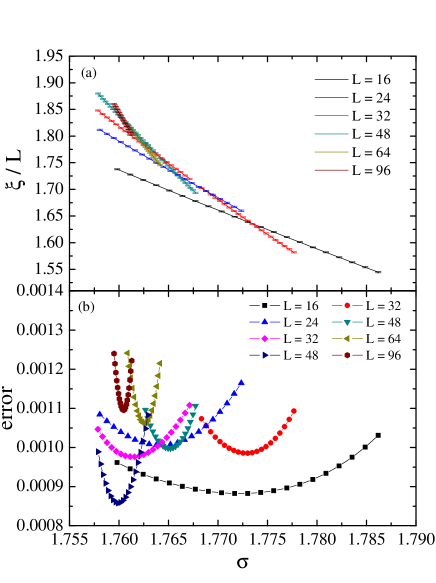
Figure 1: (Color online) (a) For several system sizes, we show $\xi/L$ as a function of the strength of the Poissonian random field $\sigma$. Lines join data obtained from reweighting extrapolation (discontinuous lines of the same color come from independent simulations). In the large-$L$ limit, $\xi/L$ is $L$-independent at the critical point $\sigma^{\rm(c)}$. In the quotients method, we consider the $\xi/L$ curves for pair of lattices $(L,2L)$ and seek the $\sigma$ where they cross. This crossing is employed for computing effective, $L$-dependent critical exponents with Eq. (69). (b) Illustration of statistical errors in the universal ratio $\xi/L$ for the pairs of the system sizes shown in panel (a).

Instead for disconnected observables (e.g. $E_{\rm J}$, connected propagators, etc.) the reweighting formulae take the standard form

$$\left.\overline{{\cal F}}\right|_{\sigma+\delta\sigma}=\left.\overline{{\cal F}{\cal R}_{\delta h_{R}}}\right|_{\sigma}\,,\ \left.D_{\sigma}\overline{{\cal F}}\right|_{\sigma+\delta\sigma}=\left.\overline{{\cal F}{\cal R}_{\delta h_{R}}{\cal D}_{\delta h_{R}}}\right|_{\sigma}\,,$$ (65)

where, in this case, the derivative operator is

$${\cal D}(\{\eta_{x},\varphi_{x}\},\delta h_{R})=\frac{1}{\sigma}\sum_{x}\big{(}\eta_{x}\phi_{x}-\frac{\delta h_{R}}{\sigma}\big{)}\,.$$ (66)

Finally, we need to asses the maximum sensible size for $\delta h_{R}$. The simplest way to proceed is to compute the moments of the reweighting factor

$$\overline{{\cal R}_{\delta h_{R}}^{k}}=\mathrm{exp}\bigg{[}N\frac{k^{2}-k}{2}\frac{\delta h_{R}^{2}}{\sigma^{2}}\bigg{]}\,.$$ (67)

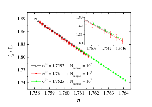
Figure 2: (Color online) Universal ratio $\xi/L$ of an $L=64$ Poissonian RFIM for three different sets of simulations, corresponding to different simulation values $\sigma^{\rm(s)}$ and different sets of random realizations. The inset is a mere enlargement of the intermediate regime of $\sigma$ values.

If we now demand the dispersion (i.e., square-root of variance) to be as large as the mean-value, we get

$$|\delta h_{R}|\leq\sigma\sqrt{\frac{\log 2}{N}}\,.$$ (68)

VII Quotients method

To extract the values of critical points, critical exponents, and dimensionless universal quantities, we employed the quotients method, also known as phenomenological renormalization Ballesteros et al. (1996); Amit and Martin-Mayor (2005); Nightingale (1976). This method allows for a particularly transparent study of corrections to scaling, that up to now have been considered as the Achilles’ heel in the study of the $D\geq 3$ random-field problem. We should note that previous applications of the method include diluted antiferromagnets Fernandez et al. (2011) and the spin-glass problem, see Ref. Baity-Jesi et al. (2013) and references therein.

We compare observables computed in pair of lattices $(L,2L)$. We start imposing scale-invariance by seeking the $L$-dependent critical point: the value of $\sigma$ ($h_{R}$ for the dG), such that $\xi_{2L}/\xi_{L}=2$ (i.e. the crossing point for $\xi_{L}/L$, see Fig. 1(a)). Now, for dimensionful quantities $O$, scaling in the thermodynamic limit as $\xi^{x_{O}/\nu}$, we consider the quotient $Q_{O}=O_{2L}/O_{L}$ at the crossing. For dimensionless magnitudes $g$, we focus on $g_{2L}$. In either case, one has:

$$Q_{O}^{\mathrm{(cross)}}=2^{x_{O}/\nu}+\mathcal{O}(L^{-\omega})\,,\ g_{(2L)}^{\mathrm{(cross)}}=g^{\ast}+\mathcal{O}(L^{-\omega})\,,$$ (69)

where $x_{O}/\nu$, $g^{\ast}$ and the scaling-corrections exponent $\omega$ are universal.

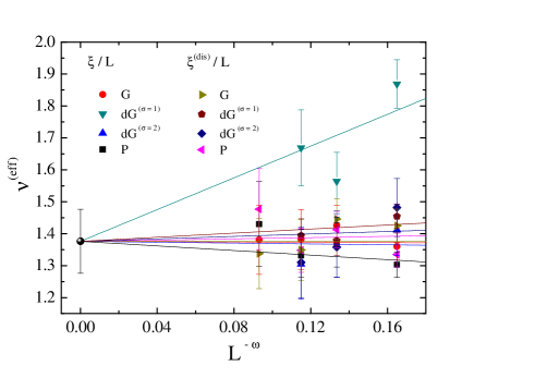
Figure 3: (Color online) Infinite limit-size extrapolation of the effective critical exponent $\nu$.

Examples of dimensionless quantities are the connected and disconnected correlation lengths over the system size, i.e., $\xi/L$ and $\xi^{\mathrm{(dis)}}/L$, and the Binder ratio $U_{4}$. Instances of dimensionful quantities are then the derivatives of $\xi$, $\xi^{\rm(dis)}$ ($x_{\xi}=1+\nu$), the connected and disconnected susceptibilities $\chi$ and $\chi^{\rm(dis)}$ [$x_{\chi}=\nu(2-\eta)$, $x_{\chi^{\rm(dis)}}=\nu(4-\bar{\eta})$], and the ratio $U_{22}$ [$x_{U_{22}}=\nu(2\eta-\bar{\eta})$] (see also Sec. IV), which as already noted above will serve as an alternative platform for investigating the validity of the so-called two-exponent scaling scenario Schwartz and Soffer (1985); Gofman et al. (1993).

Let us point out here that an extension of the quotients method using the sequence of three lattice-size points $(L,2L,4L)$ will be presented below in Sec. VIII. This generalization is necessary for the scaling study of of the bond energy of the RFIM, which is governed by a non-diverging back-ground term.

VIII Results and Discussion

Let us start with a few illustrations on the main heart of the scaling method applied, that is the crossing of the universal ratio $\xi/L$ together with the error evolution of the presented numerical scheme. As already mentioned above, we varied $\sigma$ for the Poissonian and Gaussian distributions, see panel (a) in Fig. 1, and $h_{R}$ for the double Gaussian distribution. Panel (b) in Fig. 1 shows the statistical errors of the universal ratio corresponding to the pairs of system sizes shown in panel (a) of the same figure. As expected, the error is minimal exactly at the simulation point denoted hereafter as $\sigma^{\rm(s)}$ or $h_{R}^{\rm(s)}$ respectively, and increases further away from it. Furthermore, a comparative illustration with respect to the errors induced by the reweighting method and the disorder averaging process is shown in Fig. 2 again for the universal ratio $\xi/L$ of an $L=64$ Poissonian RFIM and for three sets of simulations, as outlined in the figure. Clearly, this latter accuracy test serves in favor of the proposed scheme.

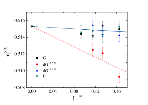
Figure 4: (Color online) Infinite limit-size extrapolation of the effective critical exponent $\eta$. Four solid lines are shown corresponding to the four random-field distributions as in Fig. 3, although they not easily discerned due to very close values of their linear coefficient terms.

The full application of Eq. (69) to our four random-field distributions has been summarized in Table II of Ref. Fytas and Martín-Mayor (2013), where all the estimates of critical points, universal ratios, and critical exponents are given, together with the corrections-to-scaling exponent $\omega=0.52(10)$ (see also Fig. 4 in Ref. Fytas and Martín-Mayor (2013)). In particular, the computation of the corrections-to-scaling exponent $\omega$ has been performed by means of a joint fit, third-order polynomial in $L^{-\omega}$, for the dimensionless quantities $\xi/L$, $\xi^{\rm(dis)}/L$, and $U_{4}$ using data for $L\geq 24$. We should point out that joint fits share the value of some fitting parameters such as the $L\to\infty$ extrapolation (which is the same for all random-field distributions), or the corrections-to-scaling exponent $\omega$ (which is common to all magnitudes). Here, we provide some complementary illustrations, showing the infinite limit-size extrapolation of the effective exponents of the correlation length $\nu$, the anomalous dimension $\eta$, and the two-exponent difference $2\eta-\bar{\eta}$, the latter serving as an independent test of the two-exponent scaling scenario in the theory of the random-field problem Schwartz and Soffer (1985).

Figures 3 and 4 illustrate the infinite limit-size extrapolation of the effective exponents $\nu$ and $\eta$ respectively, for all the four type of distributions studied. The solid lines are joint polynomial fits of first order in $L^{-\omega}$ including data points for $L\geq 32$, extrapolating to $L^{-\omega}=0$, as shown by the filled circle in each figure. We remind the reader that for the effective exponent $\nu$ we have two sets of data for each of the four distributions coming from the connected and disconnected correlation lengths Fytas and Martín-Mayor (2013). Let us comment here that our estimation $\nu=1.38(10)[3]$ is similar to the most modern computations that suggest on average a value of $1.35(7)$ Hartmann and Young (2001); Middleton (2001); Dukovski and Machta (2003); Wu and Machta (2005). For the anomalous dimension estimate $\eta=0.5153(9)[2]$, we note also $\eta=0.50(3)$ from Ref. Hartmann and Young (2001) as a comparison. Obviously, our errors for $\nu$ are larger than those for $\eta$ because we compute derivatives as connected correlations   (see also the discussion in Sec. VI).

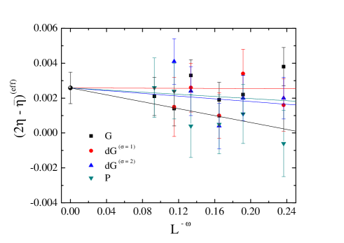
Figure 5: (Color online) Infinite limit-size extrapolation of the effective exponent $2\eta-\bar{\eta}$ .

Subsequently in Fig. 5 we perform an extrapolation of the effective exponent difference $2\eta-\bar{\eta}$, corresponding to the dimensionful quantity $U_{22}$, Eq. (13), in order to discuss the two-exponent scaling scenario. The solid lines in this figure illustrate a joint polynomial fit, first-order in $L^{-\omega}$, including data points for $L\geq 16$, giving $2\eta-\bar{\eta}=0.0026(9)[1]$ as shown by the filled black circle at $L^{-\omega}=0$. However, we should note here that if one fixes the infinite limit-size point $(2\eta-\bar{\eta})|_{L=\infty}$ to zero, the fit becomes of better quality in terms of the merit $\chi^{2}/{\rm DOF}$ Fytas and Martín-Mayor (2013). Unfortunately, in the present $D=3$ case, we can not draw a definite conclusion on the validity of the two-exponent scaling scenario. Additional work is under way to tackle this problem at higher dimensions ($D>3$) Fytas et al. (2015).

We turn our discussion now to the most controversial issue of the specific heat of the RFIM. The specific heat of the RFIM can be experimentally measured Belanger et al. (1983) and is, for sure, of great theoretical importance. Yet, it is well known that it is one of the most intricate thermodynamic quantities to deal with in numerical simulations, even when it comes to pure systems. For the RFIM, Monte Carlo methods at $T>0$ have been used to estimate the value of its critical exponent $\alpha$, but were restricted to rather small systems sizes and have also revealed many serious problems, i.e., severe violations of self averaging Parisi and Sourlas (2002); Malakis and Fytas (2006). A better picture emerged throughout the years from $T=0$ computations, proposing estimates of $\alpha\approx 0$. However, even by using the same numerical techniques, but different scaling approaches, some inconsistencies have been recorded in the literature. The most prominent was that of Ref. Hartmann and Young (2001), where a strongly negative value of the critical exponent $\alpha$ was estimated. On the other hand, experiments on random field and diluted antiferromagnetic systems suggest a clear logarithmic divergence of the specific heat Belanger et al. (1983).

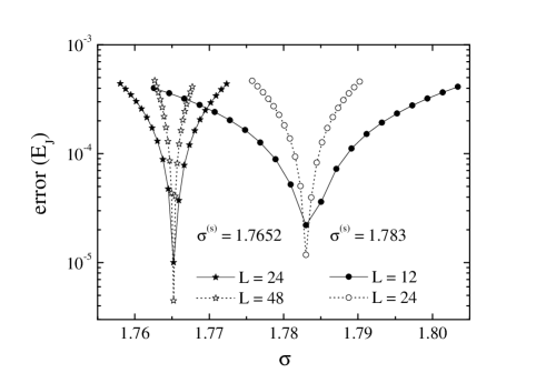
Figure 6: Semi-logarithmic illustration of statistical errors appearing in the three lattice-size variant of the quotients method. We show results for the Poissonian RFIM and $L_{1}=12$, $L_{2}=24$, and $L_{3}=48$. The values of the field strength where the simulations were performed for both pairs of system sizes are also given in the figure.

The specific heat can be estimated using ground-state calculations and applying thermodynamic relations employed by Hartmann and Young Hartmann and Young (2001) and Middleton and Fisher Middleton and Fisher (2002). The method relies on studying the singularities in the bond-energy density $E_{J}$ Holm and Janke (1997). This bond energy density is the first derivative $\partial E/\partial J$ of the ground-state energy with respect to the random-field strength, say $\sigma$ Middleton and Fisher (2002); Hartmann and Young (2001). The derivative of the sample averaged quantity $\overline{E}_{J}$ with respect to $\sigma$ then gives the second derivative with respect to $\sigma$ of the total energy and thus the sample-averaged specific heat $C$. The singularities in $C$ can also be studied by computing the singular part of $\overline{E}_{J}$, as $\overline{E}_{J}$ is just the integral of $C$ with respect to $\sigma$. The general finite-size scaling form assumed is that the singular part of the specific heat behaves as

$$C_{\rm s}\sim L^{\alpha/\nu}\tilde{C}\left[(\sigma-\sigma^{\rm(c)})L^{1/\nu}\right].$$ (70)

Thus, one may estimate $\alpha$ by studying the behavior of $\overline{E}_{J}$ at $\sigma=\sigma^{\rm(c)}$ Middleton and Fisher (2002). The computation from the behavior of $\overline{E}_{J}$ is based on integrating the above scaling equation up to $\sigma^{\rm(c)}$ , which gives a dependence of the form

$$\overline{E}_{J}(L,\sigma=\sigma^{\rm(c)})=A+BL^{(\alpha-1)/\nu},$$ (71)

with $A$ and $B$ non universal constants.

Since $\alpha-1$ is negative, Eq. (71) is dominated by the non-divergent back ground $A$, forcing us to modify the standard phenomenological renormalization. We get rid of $A$ by considering three lattice sizes in the following sequence: $(L_{1},L_{2},L_{3})=(L,2L,4L)$. We generalize Eq. (69) by taking now the quotient of the differences $Q_{O}=(O_{4L}-O_{2L})/(O_{2L}-O_{L})$ at the crossings of the pairs $(L,2L)$ and $(2L,4L)$, respectively. Applying this formula to the bond energy we obtain

$$Q_{\overline{E}_{J}}^{\mathrm{(cross)}}=2^{(\alpha-1)/\nu}+\mathcal{O}(L^{-\omega}).$$ (72)

Table 2: Effective critical exponent ratio $(\alpha-1)/\nu$ using a three lattice-size variant $(L_{1},L_{2},L_{3})=(L,2L,4L)$, see Eq. (72), of the original quotients method.

Distribution	$(L_{1},L_{2},L_{3})$	$(\alpha-1)/\nu$
G	$(12,24,48)$	-0.758(11)
	$(16,32,64)$	-0.793(17)
	$(24,48,96)$	-0.860(30)
	$(32,64,128)$	-0.881(75)
dG(σ=1)	$(16,32,64)$	0.954(66)
	$(24,48,96)$	-0.036(23)
	$(32,64,128)$	-0.309(23)
dG(σ=2)	$(12,24,48)$	-0.735(16)
	$(16,32,64)$	-0.766(16)
	$(24,48,96)$	-0.882(60)
	$(32,64,128)$	-0.867(56)
P	$(12,24,48)$	-1.120(6)
	$(16,32,64)$	-1.089(10)
	$(24,48,96)$	-1.071(42)
	$(32,64,128)$	-0.970(37)

Of course, at variance with the standard two lattice-size phenomenological renormalization, statistical errors are significantly amplified by the reweighting extrapolation, as it can be clearly seen in Fig. 6. Hence, we have preferred to carry out an independent set of simulations for parameters corresponding to the crossing points identified in the main analysis of the quotients method. Our results for the effective exponent ratio $(\alpha-1)/\nu$ are given in Table 2 and their extrapolation is shown in Fig. 7. We have excluded from the fitting procedure the data of the double Gaussian distribution with $\sigma=1$ as their inclusion destabilized the fit. The solid lines in Fig. 7 show a joint polynomial fit, second order in $L^{-\omega}$. The extrapolated value for the exponent ratio is $(\alpha-1)/\nu=-0.85(25)$ and is marked by the filled circle in the figure at $L^{-\omega}=0$. Using now our estimate $\nu=1.38(10)$ for the critical exponent of the correlation length, simple algebra (and error propagation) gives the value $\alpha=-0.16(35)$ for the critical exponent of the specific heat. Let us point out here that also Middleton and Fisher, using the scaling of the bond energy at the candidate critical field value $\sigma^{\rm(c)}=2.27$, proposed a value of $\alpha=-0.12(16)$ Middleton and Fisher (2002), compatible with our result. Although the error proposed by the latter authors is much smaller than ours, we have to note that their method implies an a priori knowledge of the “exact” value of the critical field. Obviously, as we have no command over this value, what is usually done is to use some candidate values of the critical field around the best known estimate and then repeat the simulations for all those candidate values. However, even in this case the results are ambiguous, as a change in the value of $\sigma^{\rm(c)}$ by a factor of $\delta\sigma^{\rm(c)}=10^{-3}$ results, on a average, in a change of the order of $\delta\alpha\approx 0.04$ in the value of $\alpha$ Theodorakis et al. (2013).

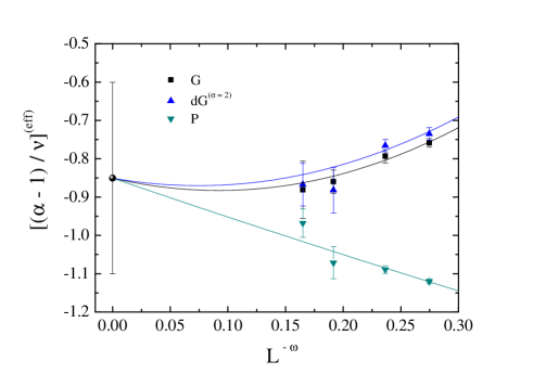
Figure 7: (Color online) Infinite limit-size extrapolation of the effective exponent ratio $(\alpha-1)/\nu$.

Following the discussion above, our numerical studies of disordered systems are carried out near their critical points using finite samples; each sample is a particular random realization of the quenched disorder. This makes it then crucial to study the dependence of some observables with the disorder, the so-called self-averaging properties of the system. The study of these properties in disordered systems has generated in the past years a large amount of works Parisi and Sourlas (2002); Aharony and Harris (1996); Chamati et al. (2002); Aharony et al. (1998); Wiseman and Domany (1998); Deroulers and Young (2002); Parisi et al. (2004); Gordillo-Guerrero and Ruiz-Lorenzo (2007), still mostly focused on the bond- and site-diluted versions of the Ising model in $D=2$ and $3$.

A typical measure of the self-averageness of a random system via a physical quantity $A$ is given from $R_{A}=[\overline{\langle A\rangle^{2}}-\overline{\langle A\rangle}^{2}]/\overline{\langle A\rangle}^{2}$. Aharony and Harris Aharony and Harris (1996) predicted that the size evolution of $R_{A}(L)$ for the random system depends on whether the system is controlled by the pure or the random fixed point, i.e., $R_{A}(L)\propto L^{(\alpha/\nu)_{\rm pure}}$ for pure fixed point, and $R_{A}(L)\propto{\rm const}\neq 0$ for random fixed point respectively, as $L\to\infty$. In the case of the random fixed point, the system has no self-averaging. On the other hand, the system exhibits weak self-averaging in the case of the pure fixed point. Clearly enough, the system is expected to be self-averaging if $R_{A}\to 0$, as $L\to\infty$.

The RFIM is a nice candidate to check the analytical predictions of Aharony and Harris on self-averaging Aharony and Harris (1996), monitoring the infinite limit-size extrapolation of $R_{A}$. In particular, we investigated here the behavior of the ratio for two observables, the connected susceptibility, $R_{\chi}$, and the bond energy, $R_{E_{J}}$. In Fig. 8 we plot the effective values of the ratios $R_{\chi}$ and $R_{E_{J}}$ in the main panel and inset, respectively, estimated at the crossing points of $\xi/L$ as usual, for all our four distributions studied, as indicated by the different colors and symbols. In both cases, the solid lines show a joint, second-order in $L^{-\omega}$ polynomial fit, using as a lower cut off the lattice size $L_{\rm min}=16$. For the case of $R_{\chi}$, the extrapolated values shown by black stars, are dependent on the field distribution and are clearly non-zero, indicating violation of self-averaging.

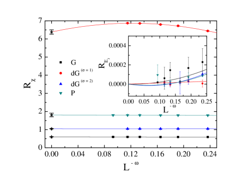
Figure 8: (Color online) Infinite limit-size extrapolation of the effective ratios $R_{\chi}$ (main panel) and $R_{E_{J}}$ (inset).

In particular, we quote the following limiting values: $R_{\chi}=\{0.600(2),\;6.38(11),\;1.047(4),\;1.81(9)\}$, for the cases of the Gaussian, double Gaussian with $\sigma=1$, double Gaussian with $\sigma=2$, and Poissonian distributions, respectively. The above results verify the prediction of Ref. Aharony and Harris (1996), according to which the susceptibility at the critical point is not self-averaging for models where the disorder is relevant, relevant meaning that the critical exponent of the specific heat of the corresponding pure model is positive ($\alpha_{\mathrm{pure}}>0$) . As for the self-averaging ratio for the bond energy, shown in Fig. 8–inset, it goes to zero with increasing system size, indicating self-averaging in the thermodynamic limit.

Finally, we present some computational aspects of the implemented push-relabel algorithm and its performance on the study of the RFIM. Although its generic implementation has a polynomial time bound, its actual performance depends on the order in which operations are performed and which heuristics are used to maintain auxiliary fields for the algorithm. Even within this polynomial time bound, there is a power-law critical slowing down of the push-relabel algorithm at the zero-temperature transition Ogielski (1986); Middleton (2002). This critical slowing down is certainly reminiscent of the slowing down seen in local algorithms of statistical mechanics at finite temperature, such as the Metropolis algorithm, and even for cluster algorithms. In fact, Ogielski Ogielski (1986) was the first to note that the push-relabel algorithm takes more time to find the ground state near the transition in three dimensions from the ferromagnetic to paramagnetic phase.

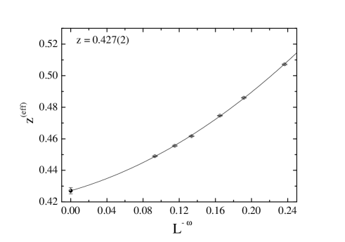
Figure 9: Infinite limit-size extrapolation of the effective exponent $z$ of the push-relabel algorithm.

A direct way to measure the dynamics of the algorithm is to examine the dependence of the running time, measured by the number of push-relabel operations, on system size $L$. Such an analysis has already been performed in Ref. Meinke and Middleton (2005) for the Gaussian $D=3$ RFIM and a FIFO queue implementation, as in the current paper, finding a dynamic exponent $z=0.43(6)$, using the data collapse technique and fixing the values $\sigma^{\rm(c)}=2.27$ and $\nu=1.37$ in the scaling ansatz. Here, we present a complementary analysis based on the numerical data also for Gaussian RFIM, using our scaling approach within the quotients method and without assuming prior knowledge of the critical field and correlation length exponent. Our fitting attempt is shown in Fig. 9, where the solid line is a second-order in $L^{-\omega}$ polynomial for system sizes $L\geq 16$ and the obtained estimate for the dynamic critical exponent $z$ is $0.427(2)$, very close to the estimate of Ref. Meinke and Middleton (2005).

IX Summary and outlook

To summarize, we have presented in the current paper a new approach to the study of the random-field Ising model, using as a platform the three-dimensional version of the model. We combined several efficient numerical methods, from zero-temperature optimization algorithms to generalized fluctuation-dissipation formulas and reweighting extrapolations that allowed the computation of response functions, as well as advanced finite-size scaling techniques that offered us the possibility to tackle some of the hardest open problems in the random-field literature, like the existence and role of scaling corrections and the universality principle of the model. We hope that this contribution gives a clear overview of all the technical details of our implementation, paving the way to even more sophisticated studies in the field of disordered systems. Currently, using the prescription outlined above, we are dealing with the random-field problem at higher dimensions and we expect to provide clear-cut results regarding the validity of the two-exponent scaling scenario, one of the building blocks in the scaling theory of the random-field Ising model.