Hadamard function and the vacuum currents in braneworlds
with compact dimensions: Two-branes geometry

Abstract

We evaluate the Hadamard function and the vacuum expectation value (VEV) of the current density for a charged scalar field in the region between two co-dimension one branes on the background of locally AdS spacetime with an arbitrary number of toroidally compactified spatial dimensions. Along compact dimensions periodicity conditions are considered with general values of the phases and on the branes Robin boundary conditions are imposed for the field operator. In addition, we assume the presence of a constant gauge field. The latter gives rise to Aharonov-Bohm type effect on the vacuum currents. There exists a range in the space of the Robin coefficients for separate branes where the vacuum state becomes unstable. Compared to the case of the standard AdS bulk, in models with compact dimensions the stability condition imposed on the parameters is less restrictive. The current density has nonzero components along compact dimensions only. These components are decomposed into the brane-free and brane-induced contributions. Different representations are provided for the latter well suited for the investigation of the near-brane, near-AdS boundary and near-AdS horizon asymptotics. The component along a given compact dimension is a periodic function of the gauge field flux, enclosed by that dimension, with the period of the flux quantum. An important feature, that distinguishes the current density from the expectation values of the field squared and energy-momentum tensor, is its finiteness on the branes. In particular, for Dirichlet boundary condition the current density vanishes on the branes. We show that, depending on the constants in the boundary conditions, the presence of the branes may either increase or decrease the current density compared with that for the brane-free geometry. Applications are given to the Randall–Sundrum 2-brane model with extra compact dimensions. In particular, we estimate the effects of the hidden brane on the current density on the visible brane.

PACS numbers: 04.62.+v, 04.50.-h, 11.10.Kk, 11.25.-w

1 Introduction

In quantum field theory the vacuum is defined as the state of a quantum field with zero number of quanta. The field operator does not commute with the operator of the number of quanta and, hence, in the vacuum state the field has no definite value. The corresponding quantum fluctuations are known as zero-point or vacuum fluctuations. The properties of these fluctuations and, hence, of the vacuum state, crucially depend on the geometry of the background spacetime (for general reviews see [1]). Not surprisingly, exact results for the physical characteristics of the vacuum can be found for highly symmetric backgrounds only. Continuing our previous research [2, 3], in this paper we investigate the changes in the properties of the vacuum state for a charged scalar field induced by three types of sources: by the curved geometry, by nontrivial topology and by boundaries.

As a background geometry we will consider locally anti-de Sitter (AdS) spacetime. AdS spacetime is the maximally symmetric solution of the vacuum Einstein equations with a negative cosmological constant and because of its high symmetry numerous physical problems are exactly solvable in this geometry. In particular, quantum field theory in AdS background has long been an active field of research. There are a number of reasons for that. Much of the early interest in the seventies was motivated by principal questions of the quantization procedure on curved backgrounds. Among the new features, having no analogues in quantum field theory on the Minkowski bulk, are the lack of global hyperbolicity and the presence of both regular and irregular modes. In addition, the natural length scale of the AdS geometry provides a convenient infrared regulator in interacting quantum field theories without reducing the number of symmetries [4]. The natural appearance of AdS spacetime as a ground state in supergravity and Kaluza-Klein theories and also as the near horizon geometry of the extremal black holes and domain walls has triggered a further increase of interest to quantum field theories on AdS bulk. This motivated the developement of a parallel line of research, i.e. that of supersymmetric field theory models in AdS background spacetime, see e.g. [5].

The AdS geometry plays the crucial role in two recent developments in high-energy physics such as the AdS/CFT correspondence and the braneworld scenario. The AdS/CFT correspondence (see, for instance, [6]) relates string theories or supergravity in the AdS bulk with a conformal field theory localized on its boundary. This duality has many interesting consequences and provides a powerful tool for the investigation of gauge field theories in the strong coupling regime. Among the recent developments of the AdS/CFT correspondence is the application to strong-coupling problems in condensed matter physics. The braneworld scenario (for reviews see [7]) offers a new perspective for the solution of the hierarchy problem between the Planck and electroweak mass scales. The main idea to resolve the large hierarchy is that the small coupling of four-dimensional gravity is generated by the large physical volume of extra dimensions. Braneworlds naturally appear in the string/M-theory context and present intriguing possibilities to solve or to address from a different point of view various problems in particle physics and cosmology.

The global geometry considered in the present paper will be different from the standard AdS one. Namely, we will assume that a part of spatial dimensions, described in Poincaré coordinates, are compactified to a torus. Note that the extra compact dimensions are an inherent feature of braneworld models arising from string and M-theories. The nontrivial topology of the background space can have important physical implications in quantum field theory. The periodicity conditions imposed on fields along compact dimensions modify the spectrum for zero-point fluctuations and, related to this, the vacuum expectation values (VEVs) of physical observables are changed. A well-known effect of this kind, demonstrating the relation between quantum phenomena and global properties of spacetime, is the topological Casimir effect [8]. The Casimir energy of bulk fields induces a nontrivial potential for the compactification radius, providing a stabilization mechanism for moduli fields and effective gauge couplings. The Casimir effect has also been considered as an origin for the dark energy in Kaluza-Klein-type and braneworld models [9].

For charged fields an important characteristic of the vacuum state is the expectation value of the current density. In addition to describing the local physical structure of the quantum field, the current acts as the source in the Maxwell equations and plays an important role in modeling a self-consistent dynamics involving the electromagnetic field. The VEV of the current density for a charged scalar field in the background of locally AdS spacetime with an arbitrary number of toroidally compactified spatial dimensions has been considered in [2] (for a recent review of quantum filed-theoretical effects in toroidal topology see [10]). Both the zero and finite temperature expectation values of the current density for charged scalar and fermionic fields in background of the flat spacetime with toroidal dimensions were investigated in [11, 12]. The vacuum current densities for charged scalar and Dirac spinor fields in de Sitter spacetime with compact spatial dimensions are considered in [13]. The effects of nontrivial topology induced by the compactification of a cosmic string along its axis have been discussed in [14].

As the third source for the vacuum polarization, we will consider two co-dimension one branes parallel to the AdS boundary. The effects induced by a single brane were studied in [3]. The influence of boundaries on the vacuum currents in topologically nontrivial flat spaces are studied in [15, 16] for scalar and fermionic fields. Note that, motivated by the problems of radion stabilization and the cosmological constant generation, the investigations of the vacuum energy and related forces for branes on AdS bulk have attracted a great deal of attention (see, for instance, the references in [17]). The Casimir effect in higher-dimensional generalizations of the AdS spacetime with compact internal spaces has been discussed in [18, 19, 20].

The organization of the paper is as follows. The next section is devoted to the description of the background geometry, the configuration of the branes, the boundary conditions, and the field content. In section 3, we evaluate the Hadamard function in the region between the branes. The single brane contributions are explicitly separated and an integral representation for the interference part is obtained well adapted for the investigation of the VEVs for physical quantities bilinear in the field operator. In section 4, the expression for the Hadamard function is used for the investigation of the vacuum current in the region between the branes. The behavior of the current density in various asymptotic regions of the parameters is discussed. Numerical examples are presented in the case when the Robin coefficients on separate branes are the same. The applications of the results to the Randall-Sundrum 2-brane model with extra compact dimensions are given in section 5. The main results of the paper are summarized in section 6. Alternative representations for the Hadamard functions, adapted for the investigation of the near-brane asymptotic of the vacuum current, are provided in Appendix.

2 Field content, bulk and boundary geometries

First we will describe the bulk geometry. The corresponding metric tensor is given by the $(D+1)$-dimensional line element

$$ds^{2}=g_{\mu\nu}dx^{\mu}dx^{\nu}=e^{-2y/a}\eta_{ik}dx^{i}dx^{k}-dy^{2},$$ (2.1)

where $i,k=0,\ldots,D-1$, $a$ is a constant, and $\eta_{ik}=\mathrm{diag}(1,-1,\ldots,-1)$ is the metric tensor for $D$-dimensional Minkowski spacetime. In addition to the $y$ coordinate, $-\infty<y\,+\infty$, we will use the coordinate $z$, defined as $z=ae^{y/a}$, $0\leqslant z<\infty$. In terms of the latter, the line element is written in a manifestly conformally flat form:

$$ds^{2}=(a/z)^{2}(\eta_{ik}dx^{i}dx^{k}-dz^{2}).$$ (2.2)

The local geometry given by (2.2) coincides with that for AdS spacetime described in Poincaré coordinates. The hypersurfaces $z=0$ and $z=\infty$ present the AdS boundary and horizon, respectively. The constant $a$ is related to the Ricci scalar by the formula $R=-D(D+1)/a^{2}$ and the metric tensor corresponding to (2.2) is a solution of the vacuum Einstein equations with a negative cosmological constant $\Lambda=-D(D-1)a^{-2}/2$.

The global properties of the geometry we are going to consider here will be different from that for AdS spacetime. We assume that the subspace normal to the $y$-coordinate has the topology $R^{p}\times T^{q}$, with $p$ and $q$ being integers such that $p+q=D-1$, and $T^{q}$ stands for a $q$-dimensional torus. So, for the ranges of the coordinates $x^{i}$ in (2.1) one has

$$-\infty < x^{i}<+\infty,\;i=1,2,\ldots,p,$$

$$0 \leqslant x^{i}\leqslant L_{i},\;i=p+1,\ldots,D-1,$$ (2.3)

with $L_{i}$ being the coordinate length of the $i$th compact dimension. Note that the proper length measured by an observer with a fixed $z$ is given by $L_{(p)i}=(a/z)L_{i}=e^{-y/a}L_{i}$. The latter decreases with increasing $y$. This feature is seen in figure 1 where we have displayed the spatial geometry in the case $D=2$, embedded into the 3-dimensional Euclidean space. The circles correspond to the compact dimension and the thick circles are the locations of the branes (see below).

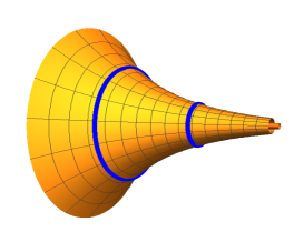
Figure 1: The spatial section of the geometry at hand for $D=2$ embedded into a 3-dimensional Euclidean space. The thick circles present the locations of the branes.

Here we are interested in the VEV of the current density for a charged scalar field $\varphi(x)$ in the background geometry specified above. In addition, we will assume the presence of an external classical gauge field $A_{\mu}$. The dynamics of the field is governed by the equation

$$\left(g^{\mu\nu}D_{\mu}D_{\nu}+m^{2}+\xi R\right)\varphi(x)=0,$$ (2.4)

where $\xi$ is the curvature coupling parameter, $D_{\mu}=\nabla_{\mu}+ieA_{\mu}$, with $\nabla_{\mu}$ being the covariant derivative operator, $m$ and $e$ are the mass and the charge of the field quanta. The most important special cases correspond to minimally and conformally coupled fields with $\xi=0$ and $\xi=(D-1)/(4D)$, respectively. The background topology is nontrivial and for the complete formulation of the problem, in addition to the field equation, the periodicity conditions should be specified along compact dimensions. Here we consider quasiperiodicity conditions

$$\varphi(t,x^{1},\ldots,x^{l}+L_{l},\ldots,y)=e^{i\alpha_{l}}\varphi(t,x^{1},\ldots,x^{l},\ldots,y),$$ (2.5)

with constant phases $\alpha_{l}$, $l=p+1,\ldots,D-1$ . As special cases, these conditions include untwisted ($\alpha_{l}=0$) and twisted ($\alpha_{l}=\pi$) scalars.

Now we turn to the description of the boundary geometry. It consists of two co-dimension one branes, located at $y=y_{1}$ and $y=y_{2}$, $y_{1}<y_{2}$, on which the field operator obeys the gauge invariant Robin boundary conditions

$$(1+\beta_{j}n_{j}^{\mu}D_{\mu})\varphi(x)=0,\quad y=y_{j},$$ (2.6)

with $j=1,2$. Here, $\beta_{1}$ and $\beta_{2}$ are constants, $n_{j}^{\mu}$ is the inward pointing (with respect to the region under consideration) normal to the brane at $y=y_{j}$. In the region between the branes, $y_{1}\leqslant y\leqslant y_{2}$, in the coordinates $(x^{i},y)$ one has $n_{j}^{\mu}=\delta_{j}\delta_{D}^{\mu}$, where $\delta_{1}=1$ and $\delta_{2}=-1$. The locations of the branes in terms of the conformal coordinate $z$ we will denote by $z_{1}$ and $z_{2}$, $z_{j}=ae^{y_{j}/a}$. For the proper distance between the branes one has $y_{2}-y_{1}=a\ln(z_{2}/z_{1})$. Boundary conditions of the type (2.6) appear in a number of physical problems, including the considerations of vacuum effects for a confined charged scalar field in external fields [21], gauge field theories, quantum gravity and supergravity [22, 23], and in models where the boundaries separate different gravitational backgrounds [24]. The Robin boundary conditions naturally arise in braneworld models (see below). A more general class of boundary conditions in the context of AdS/CFT correspondence, that include tangential derivatives of the field on the boundary, has been discussed in [25, 26]. In the corresponding approach the boundary conditions are implemented by adding the surface term in the action for a scalar field that contains a boundary kinetic term. The latter leads to the modification of the standard Klein-Gordon inner product by a boundary term. It has been shown that the appropriate choice of the surface action makes the modes with non-Dirichlet boundary conditions on the AdS boundary normalizable. However, because of the lack of a manifestly positive inner product, ghosts may appear in the bulk theory. The presence of the brane sufficiently far from the AdS boundary can serve as a mechanism to banish these ghosts [26].

In what follows we will consider the gauge field configuration with constant $A_{\mu}$. In this case, by the gauge transformation $\varphi(x)=e^{-ie\chi(x)}\varphi^{\prime}(x)$, $A_{\mu}=A_{\mu}^{\prime}+\partial_{\mu}\chi(x)$, with the function $\chi(x)=A_{\mu}x^{\mu}$, we can pass to a new gauge with the zero vector potential, $A_{\mu}^{\prime}=0$. However, the vector potential of the former gauge will not completely disappear from the problem. It will enter in the periodicity conditions for the new field operator:

$$\varphi^{\prime}(t,x^{1},\ldots,x^{l}+L_{l},\ldots,y)=e^{i\tilde{\alpha}_{l}}\varphi^{\prime}(t,x^{1},\ldots,x^{l},\ldots,y),$$ (2.7)

where

$$\tilde{\alpha}_{l}=\alpha_{l}+eA_{l}L_{l},\;l=p+1,\ldots,D-1.$$ (2.8)

Hence, the presence of a constant gauge field is equivalent to the shift in the phases of the quasiperiodicity conditions along compact dimensions. In particular, nontrivial phases are generated for untwisted and twisted scalars. The phase shift is expressed in terms of the magnetic flux $\Phi_{l}$ enclosed by the $l$th compact dimension: $eA_{l}L_{l}=-2\pi\Phi_{l}/\Phi_{0}$, with $\Phi_{0}=2\pi/e$ being the flux quantum (for physical effects of gauge field fluxes in higher dimensional models with compact dimensions see, for example, [27]).

3 Hadamard function

We are considering a free field theory (the only interactions are with the background gravitational and electromagnetic fields) and all the information on the properties of the quantum vacuum is encoded in two-point functions. As such we will choose the Hadamard function, defined as the VEV $G(x,x^{\prime})=\langle 0|\varphi(x)\varphi^{+}(x^{\prime})+\varphi^{+}(x^{\prime})\varphi(x)|0\rangle$, where $|0\rangle$ corresponds to the vacuum state. In what follows it will be assumed that the field is prepared in the Poincaré vacuum state. The latter is realized by the mode functions of the field which are obtained by solving the field equation in Poincaré coordinates corresponding to (2.1) or (2.2). The VEVs of physical observables, bilinear in the field operator, such as the energy-momentum tensor and current density, are obtained from the Hadamard function after some differentiations and limiting transition to the coincidence limit of the arguments (with an appropriate renormalization). In what follows we will present the evaluation procedure in the gauge with the fields $(\varphi^{\prime}(x),A_{\mu}^{\prime}=0)$, omitting the prime.

By expanding the field operator in terms of a complete set of positive- and negative-energy mode functions $\{\varphi_{\sigma}^{(\pm)}(x)\}$ (upper and lower signs respectively), specified by the set of quantum numbers $\sigma$ and obeying the quasiperiodicity and boundary conditions of the problem at hand, the Hadamard function can be presented as the mode sum

$$G(x,x^{\prime})=\sum_{\sigma}\sum_{s=\pm}\varphi_{\sigma}^{(s)}(x)\varphi_{\sigma}^{(s)\ast}(x^{\prime}),$$ (3.1)

where $\sum_{\sigma}$ includes the summation over the discrete quantum numbers and the integration over the continuous ones. The problem under consideration is plane symmetric and the mode function can be expressed in the factorized form

$$\varphi_{\sigma}^{(\pm)}(x)=z^{D/2}Z_{\nu}(\lambda z)e^{ik_{r}x^{r}\mp i\omega t},$$ (3.2)

where $k_{r}x^{r}=\sum_{r=1}^{D-1}k_{r}x^{r}$,

$$\omega=\sqrt{\lambda^{2}+k^{2}},\;k^{2}=\sum_{l=1}^{D-1}k_{l}^{2}.$$ (3.3)

In (3.2), $Z_{\nu}(x)$ is a cylinder function and

$$\nu=\sqrt{D^{2}/4-D(D+1)\xi+m^{2}a^{2}}.$$ (3.4)

For a conformally coupled massless scalar field $\nu=1/2$ and the problem under consideration is conformally related to the problem in Minkowski spacetime with two Robin boundaries (with the appropriate transformations of the Robin coefficients, see below and also [28] for a general plane-symmetric conformally flat bulk). In the case of imaginary values of $\nu$ the vacuum state becomes unstable [29]. In the discussion below we assume the values of the parameters for which $\nu\geqslant 0$ (Breitenlohner–Freedman bound). In particular, this is the case for minimally and conformally coupled fields.

For the components of the momentum along uncompact dimensions we have $-\infty<k_{l}<+\infty$, $l=1,\ldots,p$, and the eigenvalues for the components along compact dimensions are obtained from the conditions (2.7):

$$k_{l}=(2\pi n_{l}+\tilde{\alpha}_{l})/L_{l},\;l=p+1,\ldots,D-1,$$ (3.5)

where $n_{l}=0,\pm 1,\pm 2,\ldots$. In what follows, we will denote by $k_{(q)}^{2}$ the squared momentum in the compact subspace:

$$k_{(q)}^{2}=\sum_{l=p+1}^{D-1}k_{l}^{2}=\sum_{l=p+1}^{D-1}(2\pi n_{l}+\tilde{\alpha}_{l})^{2}/L_{l}^{2}.$$ (3.6)

Assuming that $|\tilde{\alpha}_{i}|\leqslant\pi$, for the lowest value of this momentum, denoted here by $k_{(q)}^{(0)}$, one has

$$k_{(q)}^{(0)2}=\sum_{i=p+1}^{D-1}\tilde{\alpha}_{i}^{2}/L_{i}^{2}.$$ (3.7)

In particular, for an untwisted scalar field and for the zero gauge field one has $k_{(q)}^{(0)}=0$.

The branes divide the space into three regions: $-\infty<y<y_{1}$, $y_{1}<y<y_{2}$, and $y>y_{2}$. In general, the curvature radius $a$ can be different in these three sections, as the branes may separate different phases of theory. In the braneworld scenario with two branes based on the orbifolded version of the model the region between the branes is employed only (see below). The Hadamard functions in the regions $y<y_{1}$ and $y>y_{2}$ coincide with the corresponding functions in the geometry of a single brane located at $y=y_{1}$ and $y=y_{2}$, respectively, with the same boundary conditions. The latter geometry is considered in [3] and here we will be mainly concentrated on the region between the branes, $y_{1}\leqslant y\leqslant y_{2}$. In this region, the function $Z_{\nu}(\lambda z)$ in (3.2) is a linear combination of the Bessel and Neumann functions $J_{\nu}(\lambda z)$ and $Y_{\nu}(\lambda z)$. Imposing the boundary condition (2.6) (with $D_{\mu}=\partial_{\mu}$) on the brane $y=y_{1}$ we find

$$Z_{\nu}(\lambda z)=C_{\sigma}g_{\nu}(\lambda z_{1},\lambda z),$$ (3.8)

with the function

$$g_{\nu}(u,v)=J_{\nu}(v)\bar{Y}_{\nu}^{(1)}(u)-\bar{J}_{\nu}^{(1)}(u)Y_{\nu}(v).$$ (3.9)

Here and below, for a given function $F(x)$, the notations with the bars are defined as

$$\bar{F}^{(j)}(x)=B_{j}xF^{\prime}(x)+A_{j}F(x),\quad j=1,2,$$ (3.10)

where the coefficients are given by

$$B_{j}=\delta_{j}\beta_{j}/a,\;A_{j}=1+DB_{j}/2.$$ (3.11)

Note that in the special cases $A_{j}=\pm\nu B_{j}$ one has

$$\bar{F}_{\nu}^{(j)}(x)=\pm B_{j}xF_{\nu\mp 1}(x),$$

for $F_{\nu}=J_{\nu}$ and $F_{\nu}=Y_{\nu}$. These special cases correspond to the values

$$\beta_{j}/a=-\frac{\delta_{j}}{D/2\mp\nu},$$ (3.12)

for the Robin coefficients and, hence, $B_{j}=-1/(D/2\mp\nu)$.

From the boundary condition on the brane $y=y_{2}$ it follows that the eigenvalues of $\lambda$ are solutions of the equation

$$\bar{J}_{\nu}^{(1)}(\lambda z_{1})\bar{Y}_{\nu}^{(2)}(\lambda z_{2})-\bar{Y}_{\nu}^{(1)}(\lambda z_{1})\bar{J}_{\nu}^{(2)}(\lambda z_{2})=0.$$ (3.13)

Firstly we will assume that all the roots of this equation are real. The changes in the evaluation procedure in the case when purely imaginary eigenvalues are present for $\lambda$ will be discussed below. We denote by $\lambda=\lambda_{n}$, $\lambda_{n}<\lambda_{n+1}$, $n=1,2,\ldots$, the positive roots of (3.13). Note that, for a fixed interbrane distance $y_{2}-y_{1}$ and Robin coefficients $\beta_{j}$, the product $z_{1}\lambda_{n}$ does not depend on the location of the branes and on the lengths of compact dimensions. The set of quantum numbers $\sigma$ specifying the mode functions are given by $\sigma=(n,\mathbf{k}_{p},\mathbf{n}_{q})$, where $\mathbf{k}_{p}=(k_{1},\ldots,k_{p})$ is the momentum in the non-compact subspace and $\mathbf{n}_{q}=(n_{p+1},\ldots,n_{D-1})$ determines the momentum in the compact subspace. The normalization coefficient $C_{\sigma}$ in (3.8) is found from the condition

$$\int d^{D}x\,\sqrt{|g|}g^{00}\varphi_{\sigma}^{(s)}(x)\varphi_{\sigma^{\prime}}^{(s^{\prime})\ast}(x)=\frac{\delta_{ss^{\prime}}}{2\omega}\delta_{nn^{\prime}}\delta(\mathbf{k}_{p}-\mathbf{k}_{p}^{\prime})\delta_{\mathbf{n}_{q},\mathbf{n}_{q}^{\prime}},$$ (3.14)

where $s,s^{\prime}=+,-$ and the $y$-integration goes over the region between the branes, $y_{1}\leqslant y\leqslant y_{2}$. By taking into account that the function $g_{\nu}(\lambda z_{1},\lambda z)$ is a cylinder function of the order $\nu$ with respect to the second argument (containing the integration variable) and using the standard integral for the square of the cylinder functions (see, for instance, [30]) we get the following result

$$|C_{\sigma}|^{2}=\frac{\pi^{2}\lambda_{n}T_{\nu}(\chi,z_{1}\lambda_{n})}{4\omega a^{D-1}\left(2\pi\right)^{p}V_{q}z_{1}},\quad\chi=\frac{z_{2}}{z_{1}},$$ (3.15)

where we have introduced the notation

$$T_{\nu}(\chi,u)=u\left\{\frac{\bar{J}_{\nu}^{(1)2}(u)}{\bar{J}_{\nu}^{(2)2}(\chi u)}\left[(\chi^{2}u^{2}-\nu^{2})B_{2}^{2}+A_{2}^{2}\right]-(u^{2}-\nu^{2})B_{1}^{2}-A_{1}^{2}\right\}^{-1}.$$ (3.16)

In (3.15), $V_{q}=L_{p+1}\cdots L_{D-1}$ is the volume of the compact subspace.

Substituting the mode functions into (3.1), the Hadamard function is presented in the form

$$G(x,x^{\prime}) = \frac{a^{1-D}(zz^{\prime})^{D/2}}{2^{p+1}\pi^{p-2}V_{q}z_{1}}\sum_{\mathbf{n}_{q}}\int d\mathbf{k}_{p}\,e^{ik_{r}\Delta x^{r}}\sum_{n=1}^{\infty}\frac{\lambda_{n}}{\omega_{n}}$$ (3.17)

$$\times T_{\nu}(\chi,z_{1}\lambda_{n})g_{\nu}(\lambda_{n}z_{1},\lambda_{n}z)g_{\nu}(\lambda_{n}z_{1},\lambda_{n}z^{\prime})\cos(\omega_{n}\Delta t),$$

where $\Delta x^{r}=x^{r}-x^{\prime r}$, $\Delta t=t-t^{\prime}$, and $\omega_{n}=\sqrt{\lambda_{n}^{2}+k^{2}}$. The eigenvalues $\lambda_{n}$ are given implicitly, as roots of (3.13), and for that reason this representation is not well adapted for the evaluation of the VEVs. Another drawback is that the terms in the series with large $n$ are highly oscillatory. A more convenient representation, free of these disadvantages, is obtained by making use of the generalized Abel-Plana formula [31, 32]

$$\sum_{n=1}^{\infty}h(z_{1}\lambda_{n})T_{\nu}(\chi,z_{1}\lambda_{n}) = \frac{2}{\pi^{2}}\int_{0}^{\infty}\frac{h(x)dx}{\bar{J}_{\nu}^{(1)2}(x)+\bar{Y}_{\nu}^{(1)2}(x)}$$ (3.18)

$$- \frac{1}{2\pi}\int_{0}^{\infty}dx\,\Omega_{1\nu}(x,\chi x)\left[h(ix)+h(-ix)\right],$$

with the notations

$$\Omega_{1\nu}(u,v)=\frac{\bar{K}_{\nu}^{(2)}(v)}{\bar{K}_{\nu}^{(1)}(u)F(u,v)},$$ (3.19)

and

$$F(u,v)=\bar{K}_{\nu}^{(1)}(u)\bar{I}_{\nu}^{(2)}(v)-\bar{K}_{\nu}^{(2)}(v)\bar{I}_{\nu}^{(1)}(u).$$ (3.20)

Here, $I_{\nu}(u)$ and $K_{\nu}(u)$ are the modified Bessel functions and for the functions with the bars we use the notation defined by (3.10). In the case of the function $h(x)$ corresponding to (3.17), the conditions of the validity for (3.18) are satisfied if $z+z^{\prime}+|\Delta t|<2z_{2}$. Note that in the coincidence limit and in the region between the branes this condition is satisfied for points away from the brane at $z=z_{2}$.

Let us denote by $G_{1}^{(1)}(x,x^{\prime})$ the contribution to the Hadamard function coming from the first term in the right hand-side of (3.18):

$$G_{1}^{(1)}(x,x^{\prime}) = \frac{\left(zz^{\prime}\right)^{D/2}}{\left(2\pi\right)^{p}a^{D-1}V_{q}}\sum_{\mathbf{n}_{q}}\int d\mathbf{k}_{p}\,e^{ik_{r}\Delta x^{r}}\int_{0}^{\infty}d\lambda\,\lambda$$ (3.21)

$$\times\frac{\cos(\Delta t\sqrt{\lambda^{2}+k^{2}})}{\sqrt{\lambda^{2}+k^{2}}}\frac{g_{\nu}(\lambda z_{1},\lambda z)g_{\nu}(\lambda z_{1},\lambda z^{\prime})}{\bar{J}_{\nu}^{(1)2}(\lambda z_{1})+\bar{Y}_{\nu}^{(1)2}(\lambda z_{1})}.$$

It coincides with the Hadamard function in the region $z>z_{1}$ in the geometry of a single brane at $z=z_{1}$ and has been investigated in [3]. As a result, the application of (3.18) leads to the representation

$$G(x,x^{\prime}) = G_{1}^{(1)}(x,x^{\prime})-\frac{4(zz^{\prime})^{D/2}}{\left(2\pi\right)^{p+1}a^{D-1}V_{q}}\sum_{\mathbf{n}_{q}}\int d\mathbf{k}_{p}\,e^{ik_{r}\Delta x^{r}}\int_{k}^{\infty}du\,u$$ (3.22)

$$\times\frac{\Omega_{1\nu}(uz_{1},uz_{2})}{\sqrt{u^{2}-k^{2}}}X_{\nu}^{(1)}(uz_{1},uz)X_{\nu}^{(1)}(uz_{1},uz^{\prime})\cosh(\Delta t\sqrt{u^{2}-k^{2}}),$$

where

$$X_{\nu}^{(j)}(u,v)=I_{\nu}(v)\bar{K}_{\nu}^{(j)}(u)-\bar{I}_{\nu}^{(j)}(u)K_{\nu}(v),\;j=1,2.$$ (3.23)

For special values (3.12) of the Robin coefficients one has

$$\bar{I}_{\nu}^{(j)}(x)=B_{j}xI_{\nu\mp 1}(x),\;\bar{K}_{\nu}^{(j)}(x)=-B_{j}xK_{\nu\mp 1}(x),$$ (3.24)

with $B_{j}=-1/(D/2\mp\nu)$. The second term in the right-hand side of (3.22) is induced by the presence of the brane at $z=z_{2}$. Note that, extracting the Hadamard function for the bulk in the absence of the branes, $G_{0}(x,x^{\prime})$, the function (3.21) is expressed as [3]

$$G_{1}^{(1)}(x,x^{\prime}) = G_{0}(x,x^{\prime})-\frac{4\left(zz^{\prime}\right)^{D/2}}{\left(2\pi\right)^{p+1}a^{D-1}V_{q}}\sum_{\mathbf{n}_{q}}\int d\mathbf{k}_{p}\,e^{ik_{r}\Delta x^{r}}\,\int_{k}^{\infty}du\,$$ (3.25)

$$\times u\frac{\cosh(\Delta t\sqrt{u^{2}-k^{2}})}{\sqrt{u^{2}-k^{2}}}\frac{\bar{I}_{\nu}^{(1)}(uz_{1})}{\bar{K}_{\nu}^{(1)}(uz_{1})}K_{\nu}(uz)K_{\nu}(uz^{\prime}),$$

with the last term being the brane-induced contribution.

Another representation for the Hadamard function is obtained by using the identity

$$\frac{\bar{K}_{\nu}^{(2)}(uz_{2})}{\bar{I}_{\nu}^{(2)}(uz_{2})}I_{\nu}(uz)I_{\nu}(uz^{\prime})-\frac{\bar{I}_{\nu}^{(1)}(uz_{1})}{\bar{K}_{\nu}^{(1)}(uz_{1})}K_{\nu}(uz)K_{\nu}(uz^{\prime})$$

$$\qquad=\sum_{j=1,2}\delta_{j}\Omega_{j\nu}(uz_{1},uz_{2})X_{\nu}^{(j)}(uz_{j},uz)X_{\nu}^{(j)}(uz_{j},uz^{\prime}),$$ (3.26)

where

$$\Omega_{2\nu}(u,v)=\frac{\bar{I}_{\nu}^{(1)}(u)}{\bar{I}_{\nu}^{(2)}(v)F(u,v)}.$$ (3.27)

Combining this with the expressions (3.22) and (3.25), one gets

$$G(x,x^{\prime}) = G_{1}^{(2)}(x,x^{\prime})-\frac{a^{1-D}(zz^{\prime})^{D/2}}{2^{p-1}\pi^{p+1}V_{q}}\sum_{\mathbf{n}_{q}}\int d\mathbf{k}_{p}\,e^{ik_{r}\Delta x^{r}}\int_{k}^{\infty}du\,u$$ (3.28)

$$\times\frac{\Omega_{2\nu}(uz_{1},uz_{2})}{\sqrt{u^{2}-k^{2}}}X_{\nu}^{(2)}(uz_{2},uz)X_{\nu}^{(2)}(uz_{2},uz^{\prime})\cosh(\Delta t\sqrt{u^{2}-k^{2}}).$$

In this formula, the function

$$G_{1}^{(2)}(x,x^{\prime}) = G_{0}(x,x^{\prime})-\frac{a^{1-D}(zz^{\prime})^{D/2}}{2^{p-1}\pi^{p+1}V_{q}}\sum_{\mathbf{n}_{q}}\int d\mathbf{k}_{p}\,e^{ik_{r}\Delta x^{r}}\int_{k}^{\infty}du$$ (3.29)

$$\times u\frac{\bar{K}_{\nu}^{(2)}(uz_{2})}{\bar{I}_{\nu}^{(2)}(uz_{2})}\frac{I_{\nu}(uz)I_{\nu}(uz^{\prime})}{\sqrt{u^{2}-k^{2}}}\cosh(\sqrt{u^{2}-k^{2}}\Delta t)$$

is the Hadamard function in the geometry of a single brane at $y=y_{2}$ when the brane $y=y_{1}$ is absent (see also [3]).

In the discussion above we have assumed that all the roots $\lambda$ of the equation (3.13) are real. However, depending on the values of the coefficients in the Robin boundary conditions on the branes, this equation can have purely imaginary roots, $\lambda=i\eta$, $\eta>0$ (for some special cases see below). For the corresponding modes the mode functions are given by the expression

$$\varphi_{(\mathrm{im})\sigma}^{(\pm)}(x)=C_{\sigma}^{(\mathrm{im})}z^{D/2}X_{\nu}^{(1)}(\eta z_{1},\eta z)e^{ik_{r}x^{r}\mp i\omega(\eta)t},$$ (3.30)

where $\omega(\eta)=\sqrt{k^{2}-\eta^{2}}$ and the function $X_{\nu}^{(1)}(\eta z_{1},\eta z)$ is defined by (3.23). If $\eta>k_{(q)}^{(0)}$, then for the modes with $k_{(q)}^{(0)}\leqslant k<\eta$ the energy is purely imaginary and the vacuum state becomes unstable. In order to escape this instability, we will assume that

$$\eta<k_{(q)}^{(0)}.$$ (3.31)

Note that in the absence of compact dimensions any imaginary root for the eigenvalue equation would lead to the vacuum instability. Hence, in models with compact dimensions the constraints given by the stability condition are less restrictive. The functions (3.30) obey the boundary condition on the brane at $y=y_{1}$. From the boundary condition on the second brane it follows that $\eta$ is the root of the equation

$$F(\eta z_{1},\eta z_{2})=0,$$ (3.32)

with the function $F(u,v)$ defined by the expression (3.20). Of course, this equation could directly be obtained from (3.13).

By using the integration formula

$$\int_{\eta z_{1}}^{\eta z_{2}}du\,uX_{\nu}^{(1)2}(\eta z_{1},u)=\frac{1}{2}\left[(u^{2}+\nu^{2})X_{\nu}^{(1)2}(\eta z_{1},u)-u^{2}(\partial_{u}X_{\nu}^{(1)}(\eta z_{1},u))^{2}\right]_{\eta z_{1}}^{\eta z_{2}},$$ (3.33)

from the normalization condition (3.14) (with the replacement $\delta_{nn^{\prime}}\rightarrow\delta_{\eta\eta^{\prime}}$) for the coefficient in (3.30) we find the expression

$$|C_{\sigma}^{(\mathrm{im})}|^{2}=\frac{(2\pi)^{-p}a^{1-D}\eta^{2}}{V_{q}\omega(\eta)\bar{I}_{\nu}^{(1)2}(\eta z_{1})}\left[\sum_{j=1,2}\frac{A_{j}^{2}-(\eta^{2}z_{j}^{2}+\nu^{2})B_{j}^{2}}{\delta_{j}\bar{I}_{\nu}^{(j)2}(\eta z_{j})}\right]^{-1}.$$ (3.34)

Here we have used the relations

$$X_{\nu}^{(1)}(\eta z_{1},\eta z_{1}) = -B_{1},$$

$$[\partial_{x}X_{\nu}^{(1)}(\eta z_{1},x)]_{x=\eta z_{1}} = A_{1}/(\eta z_{1}).$$ (3.35)

and

$$X_{\nu}^{(1)}(\eta z_{1},\eta z_{2}) = -B_{2}\frac{\bar{I}_{\nu}^{(1)}(\eta z_{1})}{\bar{I}_{\nu}^{(2)}(\eta z_{2})},$$

$$[\partial_{x}X_{\nu}^{(1)}(\eta z_{1},x)]_{x=\eta z_{2}} = \frac{A_{2}}{\eta z_{2}}\frac{\bar{I}_{\nu}^{(1)}(\eta z_{1})}{\bar{I}_{\nu}^{(2)}(\eta z_{2})}.$$ (3.36)

From (3.32) it follows that $\bar{I}_{\nu}^{(1)}(\eta z_{1})/\bar{I}_{\nu}^{(2)}(\eta z_{2})=\bar{K}_{\nu}^{(1)}(\eta z_{1})/\bar{K}_{\nu}^{(2)}(\eta z_{2})$ and, hence, in (3.34) we can replace the $I$-functions by the $K$-functions.

By taking into account the equation (3.32), it can be seen that

$$\sum_{j=1,2}\frac{B_{j}^{2}(\eta^{2}z_{j}^{2}+\nu^{2})-A_{j}^{2}}{\delta_{j}\bar{I}_{\nu}^{(j)2}(\eta z_{j})}=\frac{\eta\partial_{u}\left[F(uz_{1},uz_{2})\right]_{u=\eta}}{\bar{I}_{\nu}^{(1)}(\eta z_{1})\bar{I}_{\nu}^{(2)}(\eta z_{2})}.$$ (3.37)

Now, for the contribution of the modes (3.30) to the Hadamard function, by using the relation (3.37), we find the following expression

$$G_{(\mathrm{im})}(x,x^{\prime}) = -\frac{2(zz^{\prime})^{D/2}}{(2\pi)^{p}V_{q}a^{D-1}}\sum_{\mathbf{n}_{q}}\int d\mathbf{k}_{p}\,e^{ik_{r}\Delta x^{r}}\sum_{\eta}\frac{\eta}{\omega(\eta)}\frac{\overline{I}_{\nu}^{(2)}(\eta z_{2})}{\overline{I}_{\nu}^{(1)}(\eta z_{1})}$$ (3.38)

$$\times\frac{\cos[\omega(\eta)\Delta t]}{[\partial_{u}F(uz_{1},uz_{2})]_{u=\eta}}X_{\nu}^{(1)}(\eta z_{1},\eta z)X_{\nu}^{(1)}(\eta z_{1},\eta z^{\prime}).$$

The contribution to the Hadamard function from the modes with real $\lambda$ is still given by the expression (3.17). However, in the evaluation procedure by using the Abel-Plana formula differences arise compared to the case in the absence of purely imaginary roots. In the presence of the imaginary roots $\lambda=\pm i\eta$ the function used in the derivation of the Abel-Plana summation formula (see [31, 32]) has poles on the imaginary axis. These poles should be avoided by semicircles of small radius in the right half-plane. The integrals over these semicircles lead to the term

$$-\frac{i}{2}\sum_{x=\eta z_{1}}\frac{\bar{K}_{\nu}^{(2)}(\chi x)}{\bar{K}_{\nu}^{(1)}(x)}\frac{h(ix)-h(-ix)}{\partial_{x}F(x,\chi x)},$$ (3.39)

which should be added to the right-hand side of (3.18). In addition, in the presence of the imaginary roots, the second integral in (3.18) is understood in the sense of the principal value. Now, we can see that, after the application of the generalized Abel-Plana summation formula (with the additional term (3.39)) to the series over $n$ in (3.17), the part of the Hadamard function coming from the term (3.39) is equal to $-G_{(\mathrm{im})}(x,x^{\prime})$. Hence, this part cancels the contribution of the purely imaginary modes in the Hadamard function. As a result, the expressions (3.22) and (3.28) remain valid in the presence of the imaginary modes with $\eta<k_{(q)}^{(0)}$.

In addition to the modes discussed above, a mode may be present for which $\lambda=0$ and, hence, $\omega=k$.  For this mode the function $Z_{\nu}$ in (3.2) is a linear combination of $z^{\nu}$ and $z^{-\nu}$. The relative coefficient in this combination is determined from the boundary condition at $z=z_{1}$ and the mode functions are presented as

$$\varphi_{(\mathrm{s})\sigma}^{(\pm)}(x)=C_{\sigma}^{(\mathrm{s})}z^{D/2}[(z/z_{1})^{\nu}-b_{1}(z/z_{1})^{-\nu}]e^{ik_{r}x^{r}\mp ikt},$$ (3.40)

with the notation

$$b_{j}=\frac{1+\left(D/2+\nu\right)\delta_{j}\beta_{j}/a}{1+\left(D/2-\nu\right)\delta_{j}\beta_{j}/a},\;j=1,2.$$ (3.41)

Here we have assumed that $\beta_{j}/a\neq-\delta_{j}/(D/2\mp\nu)$. From the boundary condition at $z=z_{2}$ it follows that

$$b_{2}\left(z_{2}/z_{1}\right)^{2\nu}=b_{1}.$$ (3.42)

For a given interbrane distance, the equation (3.42) gives the relation between the Robin coefficients. For Dirichlet boundary condition on the branes this equation has no solutions. For Neumann boundary condition it has a solution in the case $\nu=D/2$ only and the corresponding mode function does not depend on $z$. In the Robin case, if the coefficients $\beta_{j}$ are the same for both the branes, $\beta_{1}=\beta_{2}=\beta$, the equation (3.42) has no solutions for $a/\beta\leqslant\nu-D/2$ and for these $\beta$ there are no modes with $\lambda=0$. Note that for a minimally coupled field $\nu\geqslant D/2$.

The coefficient $C_{\sigma}^{(\mathrm{s})}$ in (3.40) is determined from the normalization condition. As a result, the normalized mode functions for the special mode with $\lambda=0$ are presented in the form

$$\varphi_{(\mathrm{s})\sigma}^{(\pm)}(x)=\Omega(z)\varphi_{(\mathrm{M})\sigma}^{(\pm)}(x),$$ (3.43)

where

$$\varphi_{(\mathrm{M})\sigma}^{(\pm)}(x)=\frac{e^{ik_{r}x^{r}\mp ikt}}{\sqrt{2\left(2\pi\right)^{p}kV_{q}}},$$ (3.44)

are the mode functions for a massless scalar field in $D$-dimensional Minkowski spacetime with the spatial topology $R^{p}\times T^{q}$ and

$$\Omega(z) = z^{D/2}\frac{(z/z_{1})^{\nu}-b_{1}(z/z_{1})^{-\nu}}{a^{(D-1)/2}z_{1}}\left[\frac{b_{1}^{2}}{2\nu-2}+b_{1}\right.$$ (3.45)

$$\left.-\frac{1}{2\nu+2}-\frac{b_{1}}{b_{2}}\chi^{2}\left(\frac{b_{2}^{2}}{2\nu-2}+b_{2}-\frac{1}{2\nu+2}\right)\right]^{-1/2}.$$

In the cases $\beta_{j}/a=-\delta_{j}/(D/2\mp\nu)$ the mode functions for the special mode with $\lambda=0$ have the form (3.43) with the conformal function

$$\Omega^{2}(z)=\frac{2\left(1\mp\nu\right)z^{D\mp 2\nu}}{a^{D-1}(z_{2}^{2\mp 2\nu}-z_{1}^{2\mp 2\nu})}.$$ (3.46)

In the case $\nu=D/2$ and for Neumann boundary condition, for the mode with $\lambda=0$ one has $\varphi_{(0)\sigma}^{(\pm)}(x)=C_{\sigma}^{(\mathrm{s})}e^{ik_{r}x^{r}\mp ikt}$ and for the corresponding function $\Omega(z)$ one gets

$$\Omega^{2}(z)=\frac{\left(D-2\right)z_{1}^{D-2}}{a^{D-1}[1-(z_{1}/z_{2})^{D-2}]}.$$ (3.47)

This case will be considered in the numerical examples below.

As a consequence of the relation (3.43), the contribution of the mode with $\lambda=0$ to the Hadamard function, $G_{(\mathrm{s})}(x,x^{\prime})$, is expressed in terms of the corresponding function for a massless scalar field in $D$-dimensional Minkowski spacetime with the spatial topology $R^{p}\times T^{q}$. Denoting the latter by $G_{R^{p}\times T^{q}}^{(\mathrm{M})}(x,x^{\prime})$, one has $G_{(\mathrm{s})}(x,x^{\prime})=\Omega(z)\Omega(z^{\prime})G_{R^{p}\times T^{q}}^{(\mathrm{M})}(x,x^{\prime})$, or by making use of the expression for the Minkowskian function:

$$G_{(\mathrm{s})}(x,x^{\prime})=\frac{2\Omega(z)\Omega(z^{\prime})}{\left(2\pi\right)^{p+1/2}V_{q}}\sum_{\mathbf{n}_{q}}e^{ik_{l}\Delta x^{l}}k_{(q)}^{p-1}f_{(p-1)/2}(k_{(q)}\sqrt{\sum\nolimits_{l=1}^{p}(\Delta x^{l})^{2}-\left(\Delta t\right)^{2}}).$$ (3.48)

where $k_{l}\Delta x^{l}=\sum_{l=p+1}^{D-1}k_{l}\Delta x^{l}$, and

$$f_{\mu}(x)=x^{-\mu}K_{\mu}(x).$$ (3.49)

Note that the dependence on the mass of the field in this expression appears through the parameter $\nu$ in (3.45).

Under the condition (3.42), the contribution (3.48) coming from the special mode with $\lambda=0$ should be added to the part (3.17) for the modes with $\lambda=\lambda_{n}$. However, we can show that the representations (3.22) and (3.28) are not changed. Indeed, in the presence of the mode with $\lambda=0$ the function $h(x)$ in the generalized Abel-Plana formula (3.18) corresponding to the series over $n$ in (3.17) has a simple pole at $x=0$. Now, rotating the integration contour in the derivation of the Abel-Plana formula we should avoid this pole by arcs of a circle of small radius. The terms coming from the integrals over these arcs exactly cancel the contribution (3.48) of the special mode. As a result, the formulas (3.22) and (3.28) remain valid in the presence of the mode $\lambda=0$ as well.

4 VEV of the current density

Having the Hadamard function, one can evaluate the VEVs of various local physical observables bilinear in the field. The VEV of the energy-momentum tensor for a scalar field in the geometry with two branes is investigated in [33, 34, 35] for the background with trivial topology and in [19] for models with extra compact subspaces. Our main interest here is the VEV of the current density, $\langle 0|j_{\mu}(x)|0\rangle\equiv\langle j_{\mu}(x)\rangle$. For a charged scalar field the corresponding operator is given by the expression

$$j_{\mu}(x)=ie[\varphi^{+}(x)D_{\mu}\varphi(x)-(D_{\mu}\varphi^{+}(x))\varphi(x)].$$ (4.1)

The VEV is obtained from the Hadamard function by making use of the formula

$$\langle j_{\mu}(x)\rangle=\frac{i}{2}e\lim_{x^{\prime}\rightarrow x}(\partial_{\mu}-\partial_{\mu}^{\prime}+2ieA_{\mu})G(x,x^{\prime}),$$ (4.2)

First of all, we can see that $\langle j_{\mu}\rangle=0$ for $\mu=0,1,\ldots,p,D$. Hence, the VEVs of the charge density and of the current density components along uncompact dimensions (including the one perpendicular to the branes) vanish.

By using the expressions (3.22) and (3.28) for the Hadamard function and integrating over the momentum in the uncompact subspace, for the component of the vacuum current along the $l$th compact dimension one finds two equivalent representations

$$\langle j^{l}\rangle = \langle j^{l}\rangle_{0}+\langle j^{l}\rangle_{1}^{(j)}-\frac{eC_{p}z^{D+2}}{2^{p-1}a^{D+1}V_{q}}\sum_{\mathbf{n}_{q}}k_{l}\,\int_{k_{(q)}}^{\infty}dx\,x$$ (4.3)

$$\times(x^{2}-k_{(q)}^{2})^{(p-1)/2}\Omega_{j\nu}(xz_{1},xz_{2})X_{\nu}^{(j)2}(xz_{j},xz),$$

with $j=1,2$ and $l=p+1,\ldots,D-1$. Here we have introduced the notation

$$C_{p}=\frac{\pi^{-(p+1)/2}}{\Gamma((p+1)/2)}.$$ (4.4)

In the formula (4.3), $\left\langle j_{l}\right\rangle_{0}$ is the current density in the absence of the branes and $\left\langle j^{l}\right\rangle_{1}^{(j)}$ is the current density induced by the presence of the brane at $y=y_{j}$ when the second brane is absent. Hence, the last term in the right-hand side can be interpreted as the contribution induced by the second brane at $y=y_{j^{\prime}}$, $j^{\prime}=1,2$, $j^{\prime}\neq j$.

The contribution $\langle j^{l}\rangle_{0}$ is investigated in [2] and is given by the expression

$$\langle j^{l}\rangle_{0} = \frac{2ea^{-1-D}L_{l}}{(2\pi)^{(D+1)/2}}\sum_{\mathbf{n}_{q}}n_{l}\sin(\tilde{\alpha}_{l}n_{l})\cos(\sum_{i\neq l}\tilde{\alpha}_{i}n_{i})$$ (4.5)

$$\times q_{\nu-1/2}^{(D+1)/2}(1+\sum_{i}n_{i}^{2}L_{i}^{2}/(2z^{2})),$$

where $q_{\alpha}^{\mu}(x)=(x^{2}-1)^{-\mu/2}e^{-i\pi\mu}Q_{\alpha}^{\mu}(x)$, with $Q_{\alpha}^{\mu}(x)$ being the associated Legendre function of the second kind. In the region $z_{1}\leqslant z\leqslant z_{2}$, for the single brane-induced parts in (4.3) one has

$$\langle j^{l}\rangle_{1}^{(1)} = -\frac{eC_{p}z^{D+2}}{2^{p-1}a^{D+1}V_{q}}\sum_{\mathbf{n}_{q}}k_{l}\int_{k_{(q)}}^{\infty}dx\,x(x^{2}-k_{(q)}^{2})^{\frac{p-1}{2}}\frac{\bar{I}_{\nu}^{(1)}(xz_{1})}{\bar{K}_{\nu}^{(1)}(xz_{1})}K_{\nu}^{2}(xz),$$

$$\langle j^{l}\rangle_{1}^{(2)} = -\frac{eC_{p}z^{D+2}}{2^{p-1}a^{D+1}V_{q}}\sum_{\mathbf{n}_{q}}k_{l}\int_{k_{(q)}}^{\infty}dx\,x(x^{2}-k_{(q)}^{2})^{\frac{p-1}{2}}\frac{\bar{K}_{\nu}^{(2)}(xz_{2})}{\bar{I}_{\nu}^{(2)}(xz_{2})}I_{\nu}^{2}(xz).$$ (4.6)

The properties of these single brane contributions are discussed in [3].

All the contributions to the VEV of the current density and, hence, the total current as well, are periodic functions of the phases $\tilde{\alpha}_{i}$ with the period equal $2\pi$. In particular, the current is a periodic function of the magnetic flux enclosed by compact dimensions with the period equal to the flux quantum. The VEV of the component for the current density along the $l$th compact dimension is an odd function of the phase $\tilde{\alpha}_{l}$ corresponding to the same direction and an even function of the remaining phases $\tilde{\alpha}_{i}$, $i\neq l$. The appearance of nonzero vacuum currents discussed here is a consequence of the nontrivial spatial topology (though influenced by the local geometry and boundaries). This is an Aharonov-Bohm type effect related to the sensitivity of the wave function phase to the global geometry. For $\tilde{\alpha}_{i}=\pi m_{i}$, with $m_{i}$ being an integer, the current density vanishes. The relation (2.8) shows two interrelated reasons for the appearance of the currents: nontrivial phases in the periodicity conditions and the magnetic flux enclosed by compact dimensions.

By taking into account the expressions for the single brane-induced parts (4.6), the total current density in the region between the branes can also be presented in the form

$$\langle j^{l}\rangle = \langle j^{l}\rangle_{0}-\frac{eC_{p}z^{D+2}}{2^{p-1}a^{D+1}V_{q}}\sum_{\mathbf{n}_{q}}k_{l}\int_{k_{(q)}}^{\infty}dx\,x$$ (4.7)

$$\times(x^{2}-k_{(q)}^{2})^{\frac{p-1}{2}}\left[\frac{\bar{K}_{\nu}^{(1)}(xz_{1})\bar{I}_{\nu}^{(2)}(xz_{2})}{\bar{K}_{\nu}^{(2)}(xz_{2})\bar{I}_{\nu}^{(1)}(xz_{1})}-1\right]^{-1}$$

$$\times\left[I_{\nu}(xz)\frac{X_{\nu}^{(1)}(xz_{1},xz)}{\bar{I}_{\nu}^{(1)}(xz_{1})}-K_{\nu}(xz)\frac{X_{\nu}^{(2)}(xz_{2},xz)}{\bar{K}_{\nu}^{(2)}(xz_{2})}\right].$$

The second term in the right-hand side is the brane-induced contribution. Alternatively, extracting the single-brane contributions we can write the following decomposition

$$\langle j^{l}\rangle=\langle j^{l}\rangle_{0}+\sum_{j=1,2}\langle j^{l}\rangle_{1}^{(j)}+\langle j^{l}\rangle_{\mathrm{int}},$$ (4.8)

with the interference part

$$\langle j^{l}\rangle_{\mathrm{int}} = -\frac{eC_{p}z^{D+2}}{2^{p-1}a^{D+1}V_{q}}\sum_{\mathbf{n}_{q}}k_{l}\,\int_{k_{(q)}}^{\infty}dx\,x$$ (4.9)

$$\times(x^{2}-k_{(q)}^{2})^{\frac{p-1}{2}}\left[\frac{\bar{K}_{\nu}^{(1)}(xz_{1})\bar{I}_{\nu}^{(2)}(xz_{2})}{\bar{I}_{\nu}^{(1)}(xz_{1})\bar{K}_{\nu}^{(2)}(xz_{2})}-1\right]^{-1}$$

$$\times\left[I_{\nu}(xz)\frac{X_{\nu}^{(2)}(xz_{2},xz)}{\bar{I}_{\nu}^{(2)}(xz_{2})}-K_{\nu}(xz)\frac{X_{\nu}^{(1)}(xz_{1},xz)}{\bar{K}_{\nu}^{(1)}(xz_{1})}\right].$$

The integrand in this expression decays exponentially in the upper limit for all points including those on the branes..

Let us consider some limiting cases of the general formulas. In the limit of the large curvature radius, $a\gg y_{j},m^{-1}$, one has $z\approx a+y$, $z_{j}\approx a+y_{j}$, and both the order and arguments of the modified Bessel functions in the integrand of (4.3) are large. By using the corresponding uniform asymptotic expansions (given, for example, in [36]), to the leading order, the result for the geometry of two parallel Robin plates on the Minkowski bulk with the topology $R^{p+1}\times T^{q}$ (see [16]) is obtained:

$$\langle j^{l}\rangle^{(\mathrm{M})} = \langle j^{l}\rangle_{0}^{(\mathrm{M})}+\frac{eC_{p}}{2^{p}V_{q}}\sum_{\mathbf{n}_{q}}k_{l}\int_{\sqrt{m^{2}+k_{(q)}^{2}}}^{\infty}dx\,(x^{2}-m^{2}-k_{(q)}^{2})^{\frac{p-1}{2}}$$ (4.10)

$$\times\frac{2+\sum_{j=1,2}c_{j}(x)e^{2x|y-y_{j}|}}{c_{1}(x)c_{2}(x)e^{2x(y_{2}-y_{1})}-1}.$$

where

$$c_{j}(x)=\frac{\beta_{j}x-1}{\beta_{j}x+1},\;j=1,2.$$ (4.11)

In (4.10), the current density in the boundary-free Minkowskian geometry with compact dimensions is given by the formula [14]

$$\langle j^{l}\rangle_{0}^{(\mathrm{M})}=\frac{2eL_{l}m^{D+1}}{(2\pi)^{(D+1)/2}}\sum_{\mathbf{n}_{q}}n_{l}\sin(n_{l}\tilde{\alpha}_{l})\cos(\sum_{i\neq l}\tilde{\alpha}_{i}n_{i})f_{\frac{D+1}{2}}(m(\sum_{i}n_{i}^{2}L_{i}^{2})^{1/2}),$$ (4.12)

with $f_{\mu}(x)$ defined by (3.49).

For a conformally coupled massless field one has $\nu=1/2$ and the modified Bessel functions are expressed in terms of the elementary functions. For the current density in the region between the branes one finds the expression

$$\langle j^{l}\rangle = (z/a)^{D+1}\left[\langle j^{l}\rangle_{0}^{\mathrm{(M)}}+\frac{eC_{p}}{2^{p}V_{q}}\sum_{\mathbf{n}_{q}}k_{l}\int_{k_{(q)}}^{\infty}dx\,\right.$$ (4.13)

$$\times\left.(x^{2}-k_{(q)}^{2})^{\frac{p-1}{2}}\frac{2+\sum_{j=1,2}\tilde{c}_{j}(xz_{j})e^{2x|z-z_{j}|}}{\tilde{c}_{1}(xz_{1})\tilde{c}_{2}(xz_{2})e^{2x(z_{2}-z_{1})}-1}\right],$$

where we have introduced the notation

$$\tilde{c}_{j}(u)=\frac{u-a/\beta_{j}-\delta_{j}(D-1)/2}{u+a/\beta_{j}+\delta_{j}(D-1)/2}.$$ (4.14)

Note that the expression in the square brackets of (4.13), with the functions $\tilde{c}_{j}(u)$ replaced by $c_{j}(u)$ from (4.11), coincides with the corresponding result in the region between two Robin boundaries in Minkowski bulk with spatial topology $R^{p+1}\times T^{q}$. The difference in the functions $\tilde{c}_{j}(u)$ and $c_{j}(u)$ is related to that, though the bulk geometry is conformally flat and the field equation is conformally invariant, the coefficient in the Robin boundary condition is not conformally invariant.

As it has been shown in [16] for the Minkowski bulk and in [3] for the geometry of a single brane on AdS bulk, unlike the VEVs of the field squared and of the energy-momentum tensor, the current density is finite on the branes. For the geometry under consideration, the VEV of the current density on the brane is obtained from (4.3) with $z=z_{j}$. By taking into account that $X_{\nu}^{(j)}(xz_{j},xz_{j})=-B_{j}$, we get

$$\langle j^{l}\rangle_{z=z_{j}} = \langle j^{l}\rangle_{0}+\langle j^{l}\rangle_{1,z=z_{j}}^{(j)}-\frac{eC_{p}z_{j}^{D+2}B_{j}^{2}}{2^{p-1}a^{D+1}V_{q}}\sum_{\mathbf{n}_{q}}k_{l}\,$$ (4.15)

$$\times\int_{k_{(q)}}^{\infty}dx\,x(x^{2}-k_{(q)}^{2})^{\frac{p-1}{2}}\Omega_{j\nu}(xz_{1},xz_{2}),$$

where the last term is the current density induced by the second brane on the brane at $z=z_{j}$. For Dirichlet boundary condition the single brane and the second brane induced parts and, hence, also the total current, vanish on the branes.

In the limit when the left brane tends to the AdS boundary, $z_{1}\rightarrow 0$, one gets

$$\langle j^{l}\rangle \approx \langle j^{l}\rangle_{0}+\langle j^{l}\rangle_{1}^{(2)}-\frac{2^{2-p-2\nu}eC_{p}}{a^{D+1}V_{q}}\frac{A_{1}+B_{1}\nu}{A_{1}-B_{1}\nu}\frac{z_{1}^{2\nu}z^{D+2}}{\nu\Gamma^{2}(\nu)}\sum_{\mathbf{n}_{q}}k_{l}\,$$ (4.16)

$$\times\int_{k_{(q)}}^{\infty}dx\,x^{2\nu+1}(x^{2}-k_{(q)}^{2})^{\frac{p-1}{2}}\frac{X_{\nu}^{(2)2}(xz_{2},xz)}{\bar{I}_{\nu}^{(2)2}(xz_{2})}.$$

To the leading order we obtain the VEV in the geometry of a single brane at $z=z_{2}$. The contribution coming from the brane at $z=z_{1}$, corresponding to the last term in (4.16), decays as $z_{1}^{2\nu}$. When the right brane is close to the AdS horizon, $z_{2}\rightarrow\infty$, our starting point will be the expression (4.3) with $j=1$. In the limit under consideration one has

$$\Omega_{1\nu}(xz_{1},xz_{2})\approx(2\delta_{B_{2}0}-1)\frac{\pi e^{-2xz_{2}}}{\bar{K}_{\nu}^{(1)2}(xz_{1})}.$$ (4.17)

The dominant contribution to the integral in the right-hand side of (4.3) comes from the region near the lower limit of the integration and from the term with $\mathbf{n}_{q}=0$ with the minimal value of $k_{(q)}=k_{(q)}^{(0)}$. In the leading order one gets

$$\langle j^{l}\rangle \approx \langle j^{l}\rangle_{0}+\langle j^{l}\rangle_{1}^{(1)}+\frac{(1-2\delta_{B_{2}0})e\tilde{\alpha}_{l}z^{D+2}}{2^{p}\pi^{(p-1)/2}a^{D+1}L_{l}V_{q}}$$ (4.18)

$$\times\,\frac{X_{\nu}^{(1)2}(k_{(q)}^{(0)}z_{1},k_{(q)}^{(0)}z)}{\bar{K}_{\nu}^{(1)2}(k_{(q)}^{(0)}z_{1})e^{2k_{(q)}^{(0)}z_{2}}}(k_{(q)}^{(0)}/z_{2})^{(p+1)/2},$$

with $k_{(q)}^{(0)}z_{2}\gg 1$. Hence, when the right brane tends to the AdS horizon, its contribution to the current density, for a fixed value of $z$, is suppressed by the factor $\exp(-2k_{(q)}^{(0)}z_{2})$.

Now we turn to the asymptotics in the limiting cases for the lengths of compact dimensions. Firstly, consider the limit when the length of the one of compact dimensions, say $L_{r}$, $r\neq l$, is much larger than other length scales, $L_{r}\gg L_{i},z_{1}$. In this case the dominant contribution to the series over $n_{r}$ in (4.7) comes from large values of $|n_{r}|$ and the corresponding summation can be replaced by the integration in accordance with $\sum_{n_{r}=-\infty}^{+\infty}\rightarrow(L_{r}/\pi)\int_{0}^{\infty}dk_{r}$. Then, passing to a new integration variable $u=\sqrt{x^{2}-k_{(q)}^{2}}$ and introducing polar coordinates in the plane $(k_{r},u)$, after the integration over the angular part, we can see that, to the leading order, the result is obtained for the current density in the model where the $r$th dimension is uncompactified. In the opposite limit of small lengths of the $r$th dimension, $L_{r}\ll L_{i},z_{1}$, under the condition $|\tilde{\alpha}_{r}|<\pi$, in the expression (4.7) the contribution of the term with $n_{r}=0$ dominates. The behavior of the component of the current density along the $l$th compact dimension crucially depends whether the phase $\tilde{\alpha}_{r}$ is zero or not. In the case $\tilde{\alpha}_{r}=0$, the leading term obtained from the right-hand side coincides with the current density in the $D$-dimensional model, with the excluded $r$th compact dimension divided by $L_{(p)r}=aL_{r}/z$. Recall that the latter is the proper length of the $r$th dimension measured by an observer with the fixed coordinate $z$. For the case $\tilde{\alpha}_{r}\neq 0$, the arguments of the modified Bessel functions in the integrand of (4.7) are large. By making use of the corresponding asymptotic formulas, we can see that the contribution of the single brane at $z=z_{j}$ is suppressed by the factor $\exp(-2|\tilde{\alpha}_{r}||z-z_{j}|/L_{r})$, whereas the interference part decays as $\exp[-2|\tilde{\alpha}_{r}|(z_{2}-z_{1})/L_{r}]$.

If the length of the $l$th compact dimension is much smaller than the remaining lengths, $L_{l}\ll L_{i}$, the main contribution to the series over $\mathbf{n}_{q-1}=(n_{p+1},\ldots,n_{l-1},n_{l+1},\ldots,n_{D-1})$ in (4.3) comes from large values of $|n_{i}|$, $i=p+1,\ldots,D-1$, $i\neq l$. In this case the corresponding summation can be replaced by the integration in accordance with

$$\sum_{\mathbf{n}_{q-1}}f(k_{(q-1)})\rightarrow\frac{2^{2-q}\pi^{-(q-1)/2}V_{q}}{L_{l}\Gamma((q-1)/2)}\int_{0}^{\infty}du\,u^{q-2}f(u),$$ (4.19)

where $k_{(q-1)}^{2}=k_{(q)}^{2}-k_{l}^{2}$. As the next step, instead of $x$ we introduce a new integration variable $w=\sqrt{x^{2}-u^{2}-k_{l}^{2}}$. Passing to the polar coordinates in the plane $(u,w)$, after the evaluation of the integral over the angular variable, we find

$$\langle j^{l}\rangle \approx \langle j^{l}\rangle_{0}+\langle j^{l}\rangle_{1}^{(j)}-\frac{2^{3-D}\pi^{(1-D)/2}ez^{D+2}}{a^{D+1}L_{l}\Gamma((D-1)/2)}\sum_{n_{l}=-\infty}^{+\infty}k_{l}\,\int_{|k_{l}|}^{\infty}dx\,x$$ (4.20)

$$\times(x^{2}-k_{l}^{2})^{\frac{D-3}{2}}\Omega_{j\nu}(xz_{1},xz_{2})X_{\nu}^{(j)2}(xz_{j},xz).$$

A similar transformation is done with the single brane part $\langle j^{l}\rangle_{1}^{(j)}$ and the right-hand side of (4.20) coincides with the corresponding result in the model with a single compact dimension of the length $L_{l}$.

When, in addition to the condition $L_{l}\ll L_{i}$, one has $L_{l}\ll z_{j}$, in the integration range of (4.20) the arguments of the modified Bessel functions are large and we use the corresponding asymptotic expressions [36]. For the single brane and interference parts one gets

$$\langle j^{l}\rangle_{1}^{(j)} \approx -\gamma_{j}\frac{eL_{l}(z/L_{l})^{D+1}\mathrm{sgn}(\tilde{\alpha}_{l})}{(4\pi)^{(D-1)/2}a^{D+1}}\frac{|\tilde{\alpha}_{l}|^{(D-1)/2}e^{-2|\tilde{\alpha}_{l}||z-z_{j}|/L_{l}}}{(|z-z_{j}|/L_{l})^{(D-1)/2}},$$

$$\langle j^{l}\rangle_{\mathrm{int}} \approx \gamma_{1}\gamma_{2}\frac{2eL_{l}(z/L_{l})^{D+1}\mathrm{sgn}(\tilde{\alpha}_{l})}{(4\pi)^{(D-1)/2}a^{D+1}}\,\frac{|\tilde{\alpha}_{l}|^{(D-1)/2}e^{-2|\tilde{\alpha}_{l}|(z_{2}-z_{1})/L_{l}}}{[(z_{2}-z_{1})/L_{l}]^{(D-1)/2}},$$ (4.21)

with $L_{l}\ll|z-z_{j}|$. Here, $\gamma_{j}=2\delta_{0B_{j}}-1$ with $j=1,2$. As it is seen, both the single brane and interference contributions decay exponentially and the decay of the interference part is stronger. In the same limit, for the boundary-free part one has

$$\langle j^{l}\rangle_{0}\approx\frac{2e\Gamma((D+1)/2)}{\pi^{(D+1)/2}a^{D+1}}L_{l}(z/L_{l})^{D+1}\sum_{n=1}^{\infty}\frac{\sin(\tilde{\alpha}_{l}n)}{n^{D}},$$ (4.22)

and it dominates in the total VEV. Hence, in the limit under consideration the brane-induced parts are mainly concentrated near the branes within the range $|z-z_{j}|\lesssim L_{l}$.

Another representation for the VEV of the current density is obtained from the decomposition (A.2) for the Hadamard function, where the part $G_{l}(x,x^{\prime})$, given by (A.3), is induced by the compactification of the $l$th dimension. The first term in the right-hand side does not contribute to the current density and, after the integrations, in the absence of the modes with $\lambda^{2}<0$, for the VEV we find the following expression

$$\langle j^{l}\rangle = \frac{ea^{-1-D}z^{D+2}}{2(2\pi)^{p/2-1}V_{q}L_{l}^{p}z_{1}}\sum_{s=1}^{\infty}\frac{\sin\left(s\tilde{\alpha}_{l}\right)}{s^{p+1}}\sum_{n=1}^{\infty}\lambda_{n}T_{\nu}(\chi,\lambda_{n}z_{1})\,$$ (4.23)

$$\times g_{\nu}^{2}(\lambda_{n}z_{1},\lambda_{n}z)\sum_{\mathbf{n}_{q-1}}g_{p/2+1}(sL_{l}\sqrt{\lambda_{n}^{2}+k_{(q-1)}^{2}}),$$

with the function

$$g_{\mu}(x)=x^{\mu}K_{\mu}(x).$$ (4.24)

In the model with a single compact dimension $x^{l}$, the corresponding formula is obtained from (4.23) putting $p=D-2$, $k_{(q-1)}=0$, $V_{q}=L_{l}$ and omitting the summation $\sum_{\mathbf{n}_{q-1}}$. The vanishing of the vacuum currents on the branes in the case of Dirichlet boundary condition is explicitly seen from (4.23) by taking into account that $g_{\nu}(\lambda_{n}z_{1},\lambda_{n}z_{j})=0$ for $j=1,2$. Due to the presence of the Macdonald function, the series in the right-hand side are strongly convergent for all values of $z$. In particular, the representation (4.23) explicitly shows the finiteness of the current density on the branes. For the VEV of the current density on the brane at $z=z_{j}$ from (4.23) one gets

$$\langle j^{l}\rangle_{z=z_{j}} = -\frac{8ea^{-1-D}B_{j}^{2}z_{j}^{D+2}}{(2\pi)^{p/2+1}V_{q}L_{l}^{p}}\sum_{s=1}^{\infty}\frac{\sin\left(s\tilde{\alpha}_{l}\right)}{s^{p+1}}\sum_{n=1}^{\infty}\frac{\lambda_{n}^{2}}{\bar{J}_{\nu}^{(j)2}(z_{j}\lambda_{n})}\,$$ (4.25)

$$\times\left[\sum_{i=1,2}\frac{(z_{i}^{2}\lambda_{n}^{2}-\nu^{2})B_{i}^{2}+A_{i}^{2}}{\delta_{i}\bar{J}_{\nu}^{(i)2}(z_{i}\lambda_{n})}\right]^{-1}\sum_{\mathbf{n}_{q-1}}g_{p/2+1}(sL_{l}\sqrt{\lambda_{n}^{2}+k_{(q-1)}^{2}}),$$

for $j=1,2$.

In the presence of the modes with $\lambda^{2}\leqslant 0$ their contribution to the current density should be separately added to the right-hand side of (4.23). For the modes $\lambda=i\eta$, $\eta>0$, assuming that $\eta<k_{(q-1)}^{(0)}$, with $k_{(q-1)}^{(0)}$ being the minimal value for $k_{(q-1)}$, the corresponding contribution to the current density is formally obtained from (4.23) by making the replacements $\lambda_{n}\rightarrow i\eta$, $\sum_{n}\rightarrow\sum_{\eta}$. If $|\tilde{\alpha}_{i}|\leqslant\pi$, then one has $k_{(q-1)}^{(0)2}=\sum_{i=p+1,\neq l}^{D-1}\tilde{\alpha}_{i}^{2}/L_{i}^{2}$. For the possible special mode with $\lambda=0$ its contribution to the current density is given by the expression

$$\langle j^{l}\rangle_{(\mathrm{s})}=\frac{4e\Omega^{2}(z)(z/a)^{2}}{(2\pi)^{p/2+1}V_{q}L_{l}^{p}}\sum_{n=1}^{\infty}\frac{\sin\left(n\tilde{\alpha}_{l}\right)}{n^{p+1}}\sum_{\mathbf{n}_{q-1}}g_{p/2+1}(nL_{l}k_{(q-1)}).$$ (4.26)

The factor $(z/a)^{2}$ in this expression arises when one passes from the covariant component of the current density to the contravariant one. In models with a single compact dimension from here we get

$$\langle j^{l}\rangle_{(\mathrm{s})}=\frac{2e\Gamma(D/2)\Omega^{2}(z)(z/a)^{2}}{\pi^{D/2}L^{D-1}}\sum_{n=1}^{\infty}\frac{\sin\left(n\tilde{\alpha}_{l}\right)}{n^{D-1}}.$$ (4.27)

In particular, for Neumann boundary conditions on both the branes and for $\nu=D/2$, the factor $\Omega^{2}(z)$ does not depend on $z$ and is given by (3.47).

The representation (4.23) is well adapted for the investigation of the asymptotic behavior for large values of $L_{l}$ compared with the other length scales. In this limit one has $L_{l}\lambda_{n}\gg 1$ and the argument of the function $g_{p/2+1}(x)$ is large. The dominant contribution to the VEV comes from the mode with the lowest $\lambda_{n}$ and from the term with $s=1$. By using the asymptotic for the function $g_{p/2+1}(x)$, it is seen that the current density is suppressed by the factor $\exp(-L_{l}\sqrt{\lambda_{1}^{2}+k_{(q-1)}^{(0)2}})$. If the mode with $\lambda=0$ is present, the corresponding asymptotic directly follows from (4.26). For $k_{(q-1)}^{(0)}>0$, the contribution of the term with $n=1$ and $\mathbf{n}_{q-1}=0$ dominates and the corresponding current density decays as $\exp(-L_{l}k_{(q-1)}^{(0)})$. This decay is weaker than for the modes with positive $\lambda^{2}$. In the case $k_{(q-1)}^{(0)}=0$, the decay of the contribution of the zero mode goes down like a power-law, i.e. $1/L_{l}^{p+1}$.

The limit of small distances between the branes, compared with the AdS curvature radius, corresponds to the ratio $z_{2}/z_{1}$ close to 1. With decreasing $z_{2}/z_{1}$ the eigenvalues $\lambda_{n}$ increase and tend to infinity in the limit $z_{2}/z_{1}\rightarrow 1$. With this feature, from (4.23) it follows that the contribution of the modes with positive $\lambda^{2}$ to the VEV of the current density tends to zero in the limit when the distance between the branes tends to 0. This is not necessary to be the case for the contribution of the special mode with $\lambda=0$. For example, in the case of Neumann boundary condition and for $\nu=D/2$, the current density from the special mode is given by (4.26) with $\Omega^{2}(z)$ defined by (3.47). It diverges in the limit $z_{2}/z_{1}\rightarrow 1$.

An alternative representation for the current density in the region between the branes is obtained by using the result (A.4):

$$\langle j_{l}\rangle = \langle j^{l}\rangle_{0}+\langle j^{l}\rangle_{1}^{(1)}+\frac{4ea^{1-D}z^{D}}{(2\pi)^{p/2+1}V_{q}L_{l}^{p}}\sum_{n=1}^{\infty}\frac{\sin\left(n\tilde{\alpha}_{l}\right)}{n^{p+1}}\sum_{\mathbf{n}_{q-1}}\int_{k_{(q-1)}}^{\infty}dx\,$$ (4.28)

$$\times xw_{p/2+1}(nL_{l}\sqrt{x^{2}-k_{(q-1)}^{2}})\Omega_{1\nu}(xz_{1},xz_{2})X_{\nu}^{(1)2}(xz_{1},xz).$$

with the notation

$$w_{\nu}(x)=x^{\nu}J_{\nu}(x).$$ (4.29)

By taking into account the corresponding formula from [3] for the contribution $\langle j^{l}\rangle_{1}^{(1)}$, this expression is presented as

$$\langle j_{l}\rangle = \langle j^{l}\rangle_{0}+\frac{4ea^{1-D}z^{D}}{(2\pi)^{p/2+1}V_{q}L_{l}^{p}}\sum_{n=1}^{\infty}\frac{\sin\left(n\tilde{\alpha}_{l}\right)}{n^{p+1}}\sum_{\mathbf{n}_{q-1}}\int_{k_{(q-1)}}^{\infty}dx\,$$ (4.30)

$$\times xw_{p/2+1}(nL_{l}\sqrt{x^{2}-k_{(q-1)}^{2}})\left[\frac{\bar{K}_{\nu}^{(1)}(xz_{1})\bar{I}_{\nu}^{(2)}(xz_{2})}{\bar{K}_{\nu}^{(2)}(xz_{2})\bar{I}_{\nu}^{(1)}(xz_{1})}-1\right]^{-1}$$

$$\times\left[\frac{X_{\nu}^{(1)}(xz_{1},xz)}{\bar{I}_{\nu}^{(1)}(xz_{1})}I_{\nu}(xz)-\frac{X_{\nu}^{(2)}(xz_{2},xz)}{\bar{K}_{\nu}^{(2)}(xz_{2})}K_{\nu}(xz)\right].$$

In the presence of the mode with $\lambda^{2}<0$, the representations (4.28) and (4.30) are valid under the condition $\eta<k_{(q-1)}^{(0)}$.

In the figures below all the graphs are plotted for a minimally coupled massless scalar field in $D=4$ (except the figure in section 5, where we consider the model with $D=5$) in the model with a single compact dimension ($q=1$, $p=D-2$) of the length $L$ and with the phase $\tilde{\alpha}_{l}=\tilde{\alpha}$. For this model one has $\nu=2$ and, hence, $\nu=D/2$. As it has been discussed above, in this case for Neumann boundary condition there is a special mode with $\lambda=0$. The corresponding contribution to the current density is given by (4.27) with $\Omega^{2}(z)$ from (3.47). In the numerical examples with Robin boundary conditions we assume that the Robin coefficients for the branes are the same: $\beta_{1}=\beta_{2}\equiv\beta$. In this case there are no modes with imaginary $\lambda$ for $\beta\leqslant 0$. In order to see the behavior of the imaginary modes as a function of the Robin coefficient in the range $\beta>0$, in figure 2 we have plotted the roots of the equation (3.32), multiplied by $L$, as a function of $\beta/a$ for fixed values $z_{1}/L=0.5$ and $z_{2}/L=1$. In the range $0<\beta/a<0.2206$, for a given $\beta/a$ there are two roots. For $\beta/a>0.2206$ there is a single root which decreases with increasing $\beta/a$. For a given $\tilde{\alpha}$, the vacuum is stable if $\beta\leqslant 0$ or $\beta>\beta_{c}$ where $\beta_{c}$ is the root of the equation $L\eta(\beta/a)=\tilde{\alpha}$. This root is the abscissa of the intersection point of the left curve in figure 2 with the horizontal line $L\eta=\tilde{\alpha}$. For example, in the case $\tilde{\alpha}=\pi/2$ (in the numerical evaluations below we take this value of the phase) one has $\beta_{c}/a\approx 4.845$.

Figure 2: The imaginary modes for $\lambda$ versus the Robin coefficient for fixed values $z_{1}/L=0.5$, $z_{2}/L=1$, and $\tilde{\alpha}=\pi/2$.

In the figures we plot the graphs for the charge flux density through the $(D-1)$-dimensional spatial hypersurface $x^{l}=\mathrm{const}$. The latter is given by the quantity $n_{l}\langle j^{l}\rangle$, where $n_{l}=a/z$ is the normal to the hypersurface. This quantity is the current density measured by an observer with a fixed value for the coordinate $z$. Indeed, in order to discuss the physics from the point of view of that observer, it is convenient to introduce rescaled coordinates $x^{\prime i}=(a/z)x^{i}$. With these coordinates the warp factor in the metric for the subspace parallel to the branes is equal to one and they are physical coordinates of the observer. For the current density in these coordinates one has $\langle j^{\prime l}\rangle=(a/z)\langle j^{l}\rangle$ which is exactly the quantity presented in the graphs below. In figure 3 we have displayed the dependence of the current density on the phase $\tilde{\alpha}$ for fixed values $z_{1}/L=0.5$, $z_{2}/L=1$, $z/L=0.75$. The graphs are plotted for Dirichlet, Neumann and Robin (for $\beta/a=-1,-3$, numbers near the curves) boundary conditions. The dashed curve presents the current density in the geometry without branes. Recall that the current density is an odd periodic function of $\tilde{\alpha}$ with the period $2\pi$.

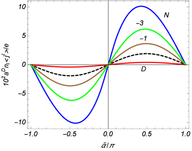
Figure 3: The vacuum current density in the region between the branes as a function of the phase in the quasiperiodicity condition along the compact dimension. The graphs are plotted for scalar fields with Dirichlet, Neumann and Robin (for $\beta/a=-1,-3$, numbers near the curves) boundary conditions and for fixed values $z_{1}/L=0.5$, $z_{2}/L=1$, $z/L=0.75$. The dashed curve corresponds to the current density in the absence of branes.

As it is seen from figure 3, for $\beta\leqslant 0$ the current density is an increasing function of $|\beta|$. In order to show the dependence of the current density on the coefficient in Robin boundary condition, in figure 4 the current density is plotted versus $\beta/a$ for $z_{1}/L=0.5$, $z_{2}/L=1$, $z/L=0.75$, and $\tilde{\alpha}=\pi/2$. As we have noted above, for these values of the parameters and in the region $0<\beta/a<4.845$ there are modes with imaginary $\lambda=i\eta$ for which $L\eta>\tilde{\alpha}$. This means that in this region the vacuum state is unstable. In figure 4, the instability region is between the ordinate axis and the dotted vertical line, corresponding to $\beta/a=4.845$. The dashed horizontal lines correspond to the current density in the cases of Ditichlet and Neumann boundary conditions. As we could expect, for large values of $|\beta|$ the results for Robin boundary condition tend to the one for Neumann condition, whereas for $\beta\rightarrow-0$ we obtain the result for Dirichlet boundary condition. For $\beta<0$ ($\beta>0$) the modulus of the current density for Robin boundary condition is smaller (larger) than that for the Neumann case.

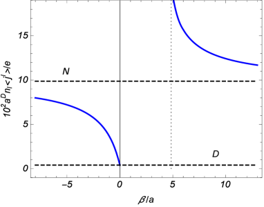
Figure 4: The VEV of the current density as a function of the Robin coefficient for $z_{1}/L=0.5$, $z_{2}/L=1$, $z/L=0.75$, and $\tilde{\alpha}=\pi/2$. The dashed lines present the current densities for Dirichlet and Neumann boundary conditions.

In figure 5, the current density is plotted in the region between the branes as a function of $z/L$ for $z_{2}/L=1$ (left panel) and $z_{2}/L=2$ (right panel). For the other parameters we have taken $z_{1}/L=0.5$, $\tilde{\alpha}=\pi/2$. The graphs are presented for Dirichlet, Neumann and for Robin boundary conditions (with the numbers near the curves being the values of $\beta/a$). For $z_{2}/L=2$ the dependence of the roots of the equation (3.32) for imaginary modes on $\beta/a$ is qualitatively similar to that depicted in figure 2. The dashed curve in the right panel corresponds to the current density in the brane-free geometry.

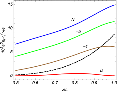
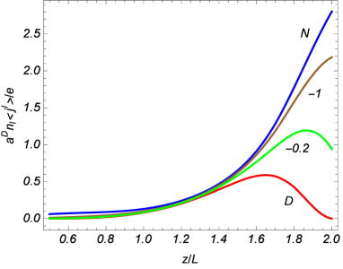
Figure 5: The current density as a function of $z/L$ for two different values of the location of the right brane: $z_{2}/L=1$ (left panel) and $z_{2}/L=2$ (right panel). The graphs are plotted for Dirichlet, Neumann and Robin (the numbers near the curves are the corresponding values of the ratio $\beta/a$) boundary conditions for fixed $z_{1}/L=0.5$, $\tilde{\alpha}=\pi/2$.

In order to show the dependence of the current density on the distance between the branes, in figure 6 the current density is displayed at a fixed point $z/L=1$ as a function of the ratio $z_{2}/L$. The horizontal dashed line corresponds to the current density in the absence of the branes. We assume that the observation point has equal proper distances from the left and right branes. This means that $z=\sqrt{z_{1}z_{2}}$ and, hence, for the example in figure 6 one has $z_{1}/L=L/z_{2}$. Under this condition the proper distance between the branes is related to the ratio $z_{2}/L$ by $y_{2}-y_{1}=2a\ln(z_{2}/L)$. Hence, the figure 6 presents the current density as a function of the proper distance between the branes at the fixed observation point in the middle between the branes. For all the boundary conditions, except the Neumann one, the current density tends to zero in the limit $y_{2}-y_{1}\rightarrow 0$. For Neumann boundary condition the current density tends to infinity. This behavior of the VEV, as a function of the interbrane distance, is in accordance with the general analysis given above. For the values of the parameters we have taken one has $\nu=D/2$ and in the case of Neumann boundary condition there is a special mode with $\lambda=0$. The contribution diverging in the zero distance limit comes from this mode. The contribution of the modes with $\lambda>0$ tends to 0 for the Neumann case as well. As it is seen from the graphs, in the case of Dirichlet boundary condition, the current density (the modulus of the current density for general $\tilde{\alpha}$) is smaller than the boundary-free part and for the Neumann case it is bigger. In particular, this means that the branes with Dirichlet (Neumann) boundary conditions suppress (enhance) the vacuum currents.

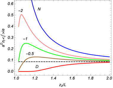
Figure 6: The current density at fixed observation point corresponding to $z/L=1$ as a function of the ratio $z_{2}/L$. The observation point has equal proper distances from the left and right branes and, hence, $z_{1}/L=L/z_{2}$.

5 Applications in Randall-Sundrum type models with compact dimensions

By using the results given above we can obtain the vacuum current densities in generalized Randall–Sundrum braneworld models [37] with extra compact dimensions. In these models the $y$-direction is compactified on an orbifold, $S^{1}/Z_{2}$, with $-b\leqslant y\leqslant b$ and with the fixed points $y=0$ and $y=b$. The latter are the locations of the hidden and visible branes, respectively. The corresponding line element is given by (2.1) with the replacement $y\rightarrow|y|$. Because of this, the Ricci scalar contains $\delta$-function terms located on the branes: $R=R_{\mathrm{AdS}}+4D[\delta(y)-\delta(y-b)]/a$. In addition, the action for a scalar field may involve the contributions of the form

$$S_{b}=-\frac{1}{2}\int d^{D+1}x\sqrt{|g|}[c_{1}\delta(y)+c_{2}\delta(y-b)]\varphi^{+}(x)\varphi(x),$$ (5.1)

where the constants $c_{1}$ and $c_{2}$ are the so-called brane mass terms. Now, the equation for the radial part of the mode functions contains the $\delta$-function terms coming from the Ricci scalar and from the brane mass terms. The boundary conditions for these functions are obtained by integrating the equation near the branes. For fields even under the reflection $y\rightarrow-y$ (untwisted scalar fields) the boundary conditions obtained in this way are of the Robin type with the coefficients (see [34, 38, 39])

$$\frac{\beta_{j}}{a}=-\frac{2}{ac_{j}+4D\xi\delta_{j}},\;j=1,2.$$ (5.2)

For odd fields (twisted scalars) Dirichlet boundary conditions are obtained on both the branes.

Now the integration over $y$ in the normalization integral (3.14) goes over the range $-b\leqslant y\leqslant b$. As a consequence of this an additional factor $1/2$ appears in the square of the normalization coefficient of the mode functions. Hence, the expressions for the VEV of the current density in the orbifolded braneworld models are obtained from those given in the previous sections with an additional factor $1/2$ and with $y_{1}=0$, $y_{2}=b$.

In braneworld models of the Randall–Sundrum type the standard model fields are located on the brane at $y=b$ (visible brane) and it is of interest to consider the current density induced by a bulk scalar field on this brane. In figure 7, in the model with $D=5$, $q=1$ (i.e. the Randall–Sundrum model with a single compact extra dimension), the current density is plotted on the visible brane, $z=z_{2}$, as a function of the location of that brane for the length of the compact dimension $L=a$. For the phase in the quasiperiodicity condition we have taken $\tilde{\alpha}=\pi/2$ and, as before, the graphs are plotted for a minimally coupled massless scalar field. The full/dashed curves correspond to Dirichlet and Neumann boundary conditions on the hidden brane. The numbers near the curves correspond to the values of $\beta_{2}/a$ (the Robin coefficient for the visible brane). In the numerical evaluations we have used the representation (4.25) with $j=2$ and with an additional factor 1/2. Note that in the case of Neumann boundary condition on both the branes the contribution of the special mode with $\lambda=0$ should be added separately. This contribution is given by (4.27) with the function $\Omega^{2}(z)$ from (3.47) and, again, with an extra factor 1/2.

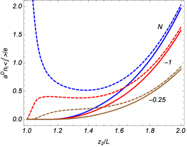
Figure 7: The current density on the visible brane for a minimally coupled massless scalar field in the Randall–Sundrum model with a single extra compact dimension as a function of the brane location. The graphs are plotted for $L=a$ and $\tilde{\alpha}=\pi/2$ in the cases of Dirichlet (full curves) and Neumann (dashed curves) boundary conditions on the hidden brane. On the visible brane, Neumann and Robin (numbers near the curves correspond to the values of $\beta_{2}/a$) boundary conditions are imposed.

In the original Randall–Sundrum 2-brane model, the hierarchy problem between the gravitational and electroweak scales is solved for the interbrane distance about 37 times larger than the AdS curvature radius $a$. In the setup we have considered this corresponds to large values of $z_{2}$ compared with $z_{1}$. If, in addition, one has $z_{2}\gg L_{i}$, the effect of the hidden brane on the current density at the location of the visible brane can be estimated by using the representation (4.15) with $j=2$. The contribution induced by the hidden brane is given by the last term in the right-hand side. The corresponding expression is simplified by taking into account that for $z_{2}\gg L_{i}$ the argument $xz_{2}$ of the modified Bessel functions is large in the integration range. The dominant contribution comes from the region near the lower limit of the integral and, under the assumption $|\tilde{\alpha}_{l}|\leqslant\pi$, from the term $\mathbf{n}_{q}=0$, corresponding to the lowest value of the momentum in the compact subspace. By using the asymptotic expressions of the modified Bessel functions for large arguments, to the leading order we find

$$\langle j^{l}\rangle_{\mathrm{RS},z=z_{2}} \approx \frac{1}{2}\langle j^{l}\rangle_{0}+\frac{1}{2}\langle j^{l}\rangle_{1}^{(2)}-\frac{e\pi^{(1-p)/2}z_{2}^{q+2}\tilde{\alpha}_{l}}{2^{p}a^{D+1}V_{q}}\,$$ (5.3)

$$\times\frac{\bar{I}_{\nu}^{(1)}(k_{(q)}^{(0)}a)}{\bar{K}_{\nu}^{(1)}(k_{(q)}^{(0)}a)}(z_{2}k_{(q)}^{(0)})^{\frac{p-1}{2}}e^{-2k_{(q)}^{(0)}z_{2}},$$

where for the location of the hidden brane we have taken $z_{1}=ae^{y_{1}/a}=a$. The contributions $\langle j^{l}\rangle_{0}$ and $\langle j^{l}\rangle_{1}^{(2)}$ are given by the formulas from the previous section with $z=z_{2}$. As is seen, the effects of the hidden brane on the visible brane are suppressed by the exponential factor $\exp(-2k_{(q)}^{(0)}z_{2})$.

6 Summary

We have investigated the combined effects of the background geometry, the nontrivial topology and the branes on the VEV of the current density for a charged scalar field with a general curvature coupling parameter. In order to have an exactly solvable problem, a highly symmetric locally AdS geometry is considered with an arbitrary number of toroidally compactified spatial dimensions. Along the compact dimensions the field obeys quasiperiodicity conditions with arbitrary constant phases and, in addition, we have assumed also the presence of a constant gauge field. By a gauge transformation, the latter is equivalent to the shift of the phases in the periodicity conditions equal to the magnetic flux enclosed by a compact dimension, measured in units of the flux quantum. As the geometry of boundaries we have considered two branes, parallel to the AdS boundary, on which the field operator obeys Robin boundary conditions, in general, with different coefficients. In the model at hand, all the properties of the vacuum state can be extracted from the two-point functions and, as the first step, we have evaluated the Hadamard function.

In the region between the branes the eigenvalues of the quantum number corresponding to the coordinate perpendicular to the branes are roots of the equation (3.13). In addition to an infinite number of modes with positive $\lambda$, depending on the coefficients in the boundary conditions on the branes, this equation may have modes with purely imaginary $\lambda=i\eta$ and also modes with $\lambda=0$. In order to escape the vacuum instability, we have assumed the condition (3.31) with $k_{(q)}^{(0)}$ being the minimal value of the momentum in the compact subspace. Note that in the corresponding models with trivial topology the presence of any mode with imaginary $\lambda$ leads to the vacuum instability. The modes with $\lambda=0$ are present under the condition (3.42) on the parameters of the model. For a given interbrane distance, this condition gives a relation between the Robin coefficients. In the expression of the Hadamard function, for the summation of the series over the positive roots of the eigenvalue equation (3.13) we have employed the generalized Abel-Plana formula. This allowed us to extract explicitly the single brane contribution and to present the second brane-induced part in terms of the integral rapidly convergent for points away from the branes. Then, we have shown that the representations (3.22) and (3.28), obtained in this way, remain valid in the presence of the modes with $\lambda^{2}\leqslant 0$ if the condition (3.31) for the stability of the vacuum is obeyed. Other representations, obtained by using the summation formula (A.1) for the series over the momentum along the $l$th compact dimension, are given in Appendix. In these representations the Hadamard function is decomposed into the contribution corresponding to the model with an uncompactified $l$th dimension and the part induced by the compactification of the latter to $S^{1}$. The first term does not contribute to the component of the current density along the $l$th dimension. The representations obtained in this way are well adapted for the investigation of the VEVs on the branes.

Given the Hadamard function, the VEV of the current density is evaluated with the help of the relation (4.2). The VEVs of the charge density and of the current components along uncompactified dimensions vanish. The component of the current density along the $l$th compact dimension is presented in two equivalent forms given by (4.3) with $j=1,2$. Another representation, in which the brane-induced contribution is presented in the form of a single integral, is provided by (4.7). The current density along the $l$th compact dimension is an odd periodic function of the phase $\tilde{\alpha}_{l}$ and an even periodic function of the remaining phases $\tilde{\alpha}_{i}$, $i\neq l$. In both cases the period is equal to $2\pi$. In particular, the current density is a periodic function of the magnetic flux having the period equal to the flux quantum. In order to clarify the behavior of the vacuum current as a function of the parameters of the model, we have considered various limiting cases. First of all, we have shown that in the limit of the large curvature radius of the background spacetime the corresponding result for the Robin plates in the Minkowski bulk with partially compactified dimensions is obtained. For a conformally coupled massless field the current density in the AdS bulk is connected to the one in the Minkowski spacetime by the conformal relation with an appropriate transformation of the Robin coefficients (see (4.13)). In the limit when the brane at $z=z_{1}$ tends to the AdS boundary, $z_{1}\rightarrow 0$, the corresponding contribution to the current density vanishes as $z_{1}^{2\nu}$ and, to the leading order, the result for the geometry of a single brane at $z=z_{2}$ is obtained. For a fixed location of the left brane, when the right brane tends to the AdS horizon, $z_{2}\rightarrow\infty$, its contribution to the vacuum current at a given observation point decays as $\exp(-2k_{(q)}^{(0)}z_{2})$. If the length of the $r$th compact dimension is much smaller than the remaining length scales and the observation point is not too close to the branes, $L_{r}\ll|z-z_{j}|$, for $0<|\tilde{\alpha}_{r}|<\pi$ the single brane contribution to the current density is suppressed by the factor $\exp(-2|\tilde{\alpha}_{r}||z-z_{j}|/L_{r})$ for the brane at $z=z_{j}$, and the interference part decays as $\exp[-2|\tilde{\alpha}_{r}|(z_{2}-z_{1})/L_{r}]$. In this limit, the current density is localized near the branes within the region $|z-z_{j}|\lesssim L_{r}$. For small values of $L_{r}$ and $\tilde{\alpha}_{r}=0$, the component of the current density along the $r$th dimension vanishes whereas the current density along other directions, to the leading order, coincides with that in the $D$-dimensional model, with the excluded $r$th compact dimension, divided by the proper length of the $r$th dimension.

For the investigation of the asymptotic for large values of the length $L_{l}$, it is more convenient to use the representation (4.23). In this limit, the contribution to the VEV of the $l$th component of the current density coming from the modes with positive $\lambda$ is suppressed by the factor $\exp(-L_{l}\sqrt{\lambda_{1}^{2}+k_{(q-1)}^{(0)2}})$. If the mode with $\lambda=0$ is present, for large values of $L_{l}$ the corresponding current density decays as $\exp(-L_{l}k_{(q-1)}^{(0)})$ in the case $k_{(q-1)}^{(0)}>0$ and as $1/L_{l}^{p+1}$ for $k_{(q-1)}^{(0)}=0$. The representation (4.23) is also well adapted for the investigation of the near-brane asymptotics of the current density. An important result seen from this representation is the finiteness of the current density on the branes. This feature is in drastic contrast compared to the cases of the VEVs for the field squared and energy-momentum tensor. It is well known that the latter diverge on the boundaries and in the evaluation of the related global quantities, like the total vacuum energy, an additional renormalization procedure is required. The current densities on the branes are directly obtained from (4.23) by putting $z=z_{j}$ and are given by the expression (4.25) with $j=1,2$ for the left and right branes, respectively. In particular, for Dirichlet boundary condition the current density and its normal derivative vanish on the branes. Another feature, seen from the expression (4.23), is that the contribution to the current density from the modes with positive $\lambda$ tends to zero in the limit of small interbrane distances.

In the numerical examples, discussed in section 4, we have considered a minimally coupled massless scalar field in the $D=4$ model with a single compact dimension and with the same Robin coefficients for the left and right branes. In this case, for $\beta\leqslant 0$ there are no modes with imaginary $\lambda$. In this range, for fixed values of the other parameters, the current density is an increasing function of $|\beta|$. In particular, it takes the minimum value for Dirichlet boundary condition and the maximum value for the Neumann one. In the range $\beta>\beta_{c}>0$, where $\beta_{c}$ is the critical value of the Robin coefficient for the stability of the vacuum (the vacuum is unstable in the range $0<\beta<\beta_{c}$), the situation is opposite: the current density decreases with increasing $\beta$.

In section 5 we have applied the general result to the 2-brane Randall–Sundrum type model with extra compact dimensions. The corresponding boundary conditions are obtained by the integration of the field equation near the branes. For untwisted scalar fields the boundary conditions are of the Robin type with the coefficients given by (5.2) with $c_{j}$ being the brane mass terms. For twisted fields Dirichlet boundary conditions are obtained. The corresponding expressions for the vacuum currents are obtained from those in section 4 with an additional coefficient $1/2$ and taking $y_{1}=0$, $y_{2}=b$. For the values of the interbrane distance solving the hierarchy problem between the electroweak and Planck scales, the current density induced by the hidden brane on the visible one is suppressed exponentially as a function of the location of the visible brane.

Appendix A Other representations for the Hadamard function

In section 3, by using the generalized Abel-Plana formula (3.18), for the Hadamard function we have provided the representation (3.22). In the expression for the VEV of the current density obtained from this representation (see (4.3)), the convergence of the integral is too slow for points near the branes and it is not convenient for the investigation of the near-brane asymptotic of the current density. Here we apply to the mode sum for the Hadamard function another type of Abel-Plana formula that allows one to extract the contribution induced by the compactification. The representation obtained in this way is well suited for the evaluation of the vacuum currents on the branes.

Let us apply to the series over $n_{l}$ in the representation (3.17) the Abel-Plana type summation formula [40]

$$\frac{2\pi}{L_{l}}\sum_{n_{l}=-\infty}^{\infty}g(k_{l})f(|k_{l}|)=\int_{0}^{\infty}du[g(u)+g(-u)]f(u)$$

$$\qquad+i\int_{0}^{\infty}du\,[f(iu)-f(-iu)]\sum_{\lambda=\pm 1}\frac{g(i\lambda u)}{e^{uL_{l}+i\lambda\tilde{\alpha}_{l}}-1},$$ (A.1)

where $k_{l}$ is given by (3.5). In the special case $g(u)=1$ and $\tilde{\alpha}_{l}=0$, this formula is reduced to the Abel-Plana formula in its standard form. The contribution of the first term in the right-hand side of (A.1) gives the Hadamard function in the geometry of two branes in $(D+1)$-dimensional locally AdS spacetime with compact dimensions $(x^{p+1},\ldots,x^{l-1},x^{l+1},\ldots,x^{D-1})$ and with the $l$th dimension being uncompactified. The latter corresponds to the spatial topology $R^{p+2}\times T^{q-1}$ and the respective Hadamard function will be denoted by $G_{R^{p+2}\times T^{q-1}}(x,x^{\prime})$. As a consequence, the Hadamard function is decomposed as

$$G(x,x^{\prime})=G_{R^{p+2}\times T^{q-1}}(x,x^{\prime})+G_{l}(x,x^{\prime}),$$ (A.2)

where the last term comes from the second integral in the right-hand side of (A.1) and is induced by the compactification of the $l$th dimension. It is presented in the form

$$G_{l}(x,x^{\prime}) = \frac{a^{1-D}L_{l}(zz^{\prime})^{D/2}}{2^{p}\pi^{p-1}V_{q}z_{1}}\sum_{s=1}^{\infty}\sum_{\mathbf{n}_{q-1}}\int d\mathbf{k}_{p}\,e^{ik_{r}\Delta x^{r}}\int_{0}^{\infty}dw\,\cosh(w\Delta t)$$ (A.3)

$$\times\sum_{n=1}^{\infty}\lambda_{n}T_{\nu}(\chi,\lambda_{n})g_{\nu}(\lambda_{n}z_{1},\lambda_{n}z)g_{\nu}(\lambda_{n}z_{1},\lambda_{n}z^{\prime})$$

$$\times\cosh\left(u\Delta x^{l}+is\tilde{\alpha}_{l}\right)\frac{e^{-suL_{l}}}{u}|_{u=\sqrt{w^{2}+\lambda_{n}^{2}+k^{(l)2}}},$$

where $\mathbf{n}_{q-1}=(n_{p+1},\ldots,n_{l-1},n_{l+1},\ldots,n_{D-1})$, $k^{(l)2}=k^{2}-k_{l}^{2}$, and the summation over $r$ in $k_{r}\Delta x^{r}$ is over $r=1,\ldots,D-1$, $r\neq l$. Note that the part (A.3) is finite in the coincidence limit of the arguments, including the points on the branes. The physical reason for this feature is related to that the toroidal compactification does not change the local geometry and the structure of the divergences is the same as that for AdS bulk without the compactification. The first term in the right-hand side (A.2) does not contribute to the component of the current density along the $l$th dimension.

Yet another representation is obtained applying to the series over $n$ in (A.3) the summation formula (3.18). This leads to the following decomposition

$$G_{l}(x,x^{\prime}) = G_{l}^{(1)}(x,x^{\prime})-\frac{8L_{l}(zz^{\prime})^{D/2}}{(2\pi)^{p+2}a^{D-1}V_{q}}\sum_{s=1}^{\infty}\sum_{\mathbf{n}_{q-1}}\int d\mathbf{k}_{p}\,e^{ik_{r}\Delta x^{r}}$$ (A.4)

$$\times\int_{0}^{\infty}dw\,\cosh(w\Delta t)\int_{0}^{\infty}dv\,\sum_{j=\pm 1}\cos\left(v\Delta x^{l}+js\tilde{\alpha}_{l}\right)e^{-ijsvL_{l}}$$

$$\times\Omega_{1\nu}(uz_{1},uz_{2})X_{\nu}^{(1)}(uz_{1},uz)X_{\nu}^{(1)}(uz_{1},uz^{\prime})|_{u=\sqrt{v^{2}+w^{2}+k^{(l)2}}}.$$

Here the term

$$G_{l}^{(1)}(x,x^{\prime}) = \frac{4\left(zz^{\prime}\right)^{D/2}L_{l}}{\left(2\pi\right)^{p+1}a^{D-1}V_{q}}\sum_{n=1}^{\infty}\sum_{\mathbf{n}_{q-1}}\int d\mathbf{k}_{p}\,e^{ik_{r}\Delta x^{r}}\int_{0}^{\infty}d\lambda\,\lambda$$ (A.5)

$$\times\frac{g_{\nu}(\lambda z_{1},\lambda z)g_{\nu}(\lambda z_{1},\lambda z^{\prime})}{\bar{J}_{\nu}^{(1)2}(\lambda z_{1})+\bar{Y}_{\nu}^{(1)2}(\lambda z_{1})}\,\int_{0}^{\infty}dw\cosh(w\Delta t)$$

$$\times\frac{e^{-nuL_{l}}}{u}\cosh(u\Delta x^{l}+in\tilde{\alpha}_{l})|_{u=\sqrt{w^{2}+\lambda^{2}+k^{(l)2}}},$$

comes from the first integral in the right-hand side of (3.18). It is the part of the Hadamard function induced by the compactification of the $l$th dimension in the geometry of a single brane at $y=y_{1}$.

References

- [1] N.D. Birrell and P.C.W. Davies, Quantum Fields in Curved Space (Cambridge University Press, Cambridge, 1982); S.A. Fulling, Aspects of Quantum Field Theory in Curved Space-time (Cambridge University Press, Cambridge, 1989); I.L. Buchbinder, S.D. Odintsov, and I.L. Shapiro, Effective Action in Quantum Gravity (Taylor & Francis, New York, 1992); A.A. Grib, S.G. Mamayev, and V.M. Mostepanenko, Vacuum Quantum Effects in Strong Fields (Friedmann Laboratory Publishing, St. Petersburg, 1994); L.E. Parker and D.J. Toms, Quantum Field Theory in Curved Spacetime (Cambridge University Press, Cambridge, 2009).
- [2] E.R. Bezerra de Mello, A.A. Saharian, and V. Vardanyan, Phys. Lett. B 741, 155 (2015).
- [3] S. Bellucci, A.A. Saharian, and V. Vardanyan, JHEP 11 (2015) 092.
- [4] C.G. Callan, Jr. and F. Wilczek, Nucl. Phys. B 340, 366 (1990).
- [5] S. Bellucci and J. Gonzalez, Phys. Rev. D 33, 619 (1986); S. Bellucci and J. Gonzalez, Phys. Rev. D 33, 2319 (1986); S. Bellucci and J. Gonzalez, Phys. Rev. D 34, 1076 (1986); S. Bellucci, Phys. Rev. D 36, 1127 (1987); S. Bellucci and J. Gonzalez, Nucl. Phys. B 302, 423 (1988); S. Bellucci and J. Gonzalez, Phys.Rev. D 37, 2357 (1988); S. Bellucci, Phys. Rev. D 57, 1057 (1998).
- [6] O. Aharony, S.S. Gubser, J. Maldacena, H. Ooguri, and Y. Oz, Phys. Rep. 323, 183 (2000).
- [7] V.A. Rubakov, Phys. Usp. 44, 871 (2001); P. Brax and C. Van de Bruck, Class. Quantum Grav. 20, R201 (2003); E. Kiritsis, Phys. Rep. 421, 105 (2005); R. Maartens and K. Koyama, Living Rev. Relativity 13, 5 (2010).
- [8] E. Elizalde, S. D. Odintsov, A. Romeo, A. A. Bytsenko, and S. Zerbini, Zeta Regularization Techniques with Applications (World Scientific, Singapore, 1994); V.M. Mostepanenko and N.N. Trunov, The Casimir Effect and its Applications (Clarendon, Oxford, 1997); K.A. Milton, The Casimir Effect: Physical Manifestation of Zero-Point Energy (World Scientific, Singapore, 2002); M. Bordag, G.L. Klimchitskaya, U. Mohideen, and V.M. Mostepanenko, Advances in the Casimir Effect (Oxford University Press, Oxford, 2009); Lecture Notes in Physics: Casimir Physics, edited by D. Dalvit, P. Milonni, D. Roberts, and F. da Rosa (Springer, Berlin, 2011), Vol. 834.
- [9] E. Elizalde, Phys. Lett. B 516, 143 (2001); C.L. Gardner, Phys. Lett. B 524, 21 (2002); K.A. Milton, Gravitation Cosmol. 9, 66 (2003); A.A. Saharian, Phys. Rev. D 70, 064026 (2004); E. Elizalde, J. Phys. A 39, 6299 (2006); A.A. Saharian, Phys. Rev. D 74, 124009 (2006); B. Green and J. Levin, JHEP 11 (2007) 096; P. Burikham, A. Chatrabhuti, P. Patcharamaneepakorn, and K. Pimsamarn, JHEP 07 (2008) 013; P. Chen, Nucl. Phys. B, Proc. Suppl. 173, s8 (2009).
- [10] F.C. Khanna, A.P.C. Malbouisson, J.M.C. Malbouisson, and A.E. Santana, Phys. Rep. 539, 135 (2014).
- [11] E.R. Bezerra de Mello and A.A. Saharian, Phys. Rev. D 87, 045015 (2013).
- [12] S. Bellucci and A.A. Saharian, Phys. Rev. D 82, 065011 (2010); S. Bellucci, E.R. Bezerra de Mello, A.A. Saharian, Phys. Rev. D 89, 085002 (2014).
- [13] S. Bellucci, A.A. Saharian, and H.A. Nersisyan, Phys. Rev. D 88, 024028 (2013).
- [14] E.R. Bezerra de Mello and A.A. Saharian, Eur. Phys. J. C. 73, 2532 (2013); S. Bellucci, E.R. Bezerra de Mello, A. de Padua, and A.A. Saharian, Eur. Phys. J. C. 74, 2688 (2014); A. Mohammadi, E.R. Bezerra de Mello, and A.A. Saharian, Class. Quantum Grav. 32, 135002 (2015).
- [15] S. Bellucci and A.A. Saharian, Phys. Rev. D 87, 025005 (2013).
- [16] S. Bellucci, A.A. Saharian, and N.A. Saharyan, Eur. Phys. J. C 75, 378 (2015).
- [17] E. Elizalde, S.D. Odintsov, and A.A. Saharian, Phys. Rev. D 87, 084003 (2013).
- [18] A. Flachi, J. Garriga, O. Pujolàs, and T. Tanaka, JHEP 08 (2003) 053; A. Flachi and O. Pujolàs, Phys. Rev. D 68, 025023 (2003).
- [19] A.A. Saharian, Phys. Rev. D 73, 044012 (2006); A.A. Saharian, Phys. Rev. D 73, 064019 (2006).
- [20] E. Elizalde, M. Minamitsuji, and W. Naylor, Phys. Rev. D 75, 064032 (2007); R. Linares, H.A. Morales-Técotl, and O. Pedraza, Phys. Rev. D 77, 066012 (2008); M. Frank, N. Saad, and I. Turan, Phys. Rev. D 78, 055014 (2008).
- [21] J. Ambjorn and S. Wolfram, Ann. Phys. (N.Y.) 147, 33 (1983).
- [22] G. Esposito, A.Yu. Kamenshchik, and G. Pollifrone, Euclidean Quantum Gravity on Manifolds with Boundary (Springer, Dordrecht, 1997); I.G. Avramidi and G. Esposito, Commun. Math. Phys. 200, 495 (1999).
- [23] H. Luckock, J. Math. Phys. 32, 1755 (1991).
- [24] S. Bellucci, A.A. Saharian, and A.H. Yeranyan, Phys. Rev. D 89, 105006 (2014); S. Bellucci, A.A. Saharian, and N.A. Saharyan, Eur. Phys. J. C 74, 3047 (2014); E.R. Bezerra de Mello and A.A. Saharian, arXiv:1408.6404, to appear in Int. J. Theor. Phys.
- [25] T. Andrade and D. Marolf, JHEP 01 (2012) 049.
- [26] T. Andrade, T. Faulkner, and D. Marolf, JHEP 05 (2012) 011.
- [27] M.R. Douglas and S. Kachru, Rev. Mod. Phys. 79, 733 (2007).
- [28] A.A. Saharian and M.R. Setare, Phys. Lett. B 552, 119 (2003).
- [29] P. Breitenlohner and D.Z. Freedman, Phys. Lett. B 115, 197 (1982); P. Breitenlohner and D.Z. Freedman, Ann. Phys. (NY) 144, 249 (1982). L. Mezincescu and P.K. Townsend, Ann. Phys. (NY) 160, 406 (1985).
- [30] A.P. Prudnikov and Yu.A. Brychkov, O.I. Marichev, Integrals and series (Gordon and Breach, New York, 1986), Vol.2.
- [31] A.A. Saharian, Izv. Akad. Nauk Arm. SSR Mat. 22, 166 (1987) [Sov. J. Contemp. Math. Anal. 22, 70 (1987)]; A.A. Saharian, The Generalized Abel-Plana Formula with Applications to Bessel Functions and Casimir Effect (Yerevan State University Publishing House, Yerevan, 2008); Report No. ICTP/2007/082; arXiv:0708.1187.
- [32] A.A. Saharian, Phys. Rev. D 63, 125007 (2001).
- [33] A.Knapman and D. J.Toms, Phys. Rev. D 69, 044023 (2004).
- [34] A.A. Saharian, Nucl. Phys. B 712, 196 (2005).
- [35] S.-H. Shao, P. Chen, and J.-A. Gu, Phys. Rev. D 81, 084036 (2010).
- [36] Handbook of Mathematical Functions, edited by M. Abramowitz and I.A. Stegun (Dover, New York, 1972).
- [37] L. Randall and R. Sundrum, Phys. Rev. Lett. 83, 3370 (1999).
- [38] T. Gherghetta and A. Pomarol, Nucl. Phys. B 586, 41 (2000).
- [39] A. Flachi and D.J. Toms, Nucl. Phys. B 610, 144 (2001).
- [40] E.R. Bezerra de Mello and A.A. Saharian, Phys. Rev. D 78, 045021 (2008); S. Bellucci, A.A. Saharian, and V.M. Bardeghyan, Phys. Rev. D 82, 065011 (2010).