Trigonal Warping in Bilayer Graphene: Energy versus Entanglement Spectrum

Abstract

We present a mainly analytical study of the entanglement spectrum of Bernal-stacked graphene bilayers in the presence of trigonal warping in the energy spectrum. Upon tracing out one layer, the entanglement spectrum shows qualitative geometric differences to the energy spectrum of a graphene monolayer. However, topological quantities such as Berry phase type contributions to Chern numbers agree. The latter analysis involves not only the eigenvalues of the entanglement Hamiltonian but also its eigenvectors.

We also discuss the entanglement spectra resulting from tracing out other sublattices. As a technical basis of our analysis we provide closed analytical expressions for the full eigensystem of bilayer graphene in the entire Brillouin zone with a trigonally warped spectrum.

I Introduction

Although first considered as a source of quantum corrections to the entropy of black holesPhysRevD.34.373 , entanglement entropy, in particular the von Neumann entropy, evolved into a tool in the field of many-body systems. This brought along connections between seemingly unrelated research areas. In condensed matter, the entanglement entropy serves, e.g., as a geometrical interpretation for the boundary between local quantum many-body systems. This connection has its origin in the area lawsRevModPhys.82.277 .

However, Li and Haldane have shown that the related entanglement spectrum contains more information than the single number expressed by the entanglement entropyLi08 . This spectrum is determined by the Schmidt decomposition of the ground state of a bipartite system, and the reduced density matrix obtained by tracing out one of the subsystems can always be formulated as

$$\rho_{\rm red}=\frac{e^{-{\cal H}_{\rm ent}}}{Z}$$ (1)

with an entanglement Hamiltonian ${\cal H}_{\rm ent}$ encoding the entanglement spectrum, and a partition function $Z={\rm tr}(e^{-{\cal H}_{\rm ent}})$. Following the Li-Haldane conjectureLi08 , in a gaped phase, the entanglement spectrum can be directly related to the spectrum of edge excitations as shown for the Fractional Quantum Hall SystemLauchli10 ; Thomale10 ; Chandran11 . This relation to the edge excitations can be also seen analytically in the case of non-interacting particles. It can be shown by mapping the free fermionic system ${\cal H}$ onto a flat-band Hamiltonian ${\cal H}_{\text{flat}}$Kitaev06 . Now, the eigenenergies $e_{i}$ of the latter are related to the eigenenergies of the corresponding entanglement energies $\varepsilon_{i}$ as $e_{i}\sim\tanh\left(\varepsilon_{i}/2\right)/2+\text{const}.$Turner10 Thereby, the eigenstates of both ${\cal H}_{\text{flat}}$ and ${\cal H}$ are the same. Thus, if ${\cal H}$ contains topologically protected surface states the same holds for the entanglement Hamiltonian.

This is why the entanglement spectrum, beyond the related entropy, is considered a tower of states and used as a fingerprint for topological order. However, this is not true in general as shown recently by A. Chandran et al., Ref. PhysRevLett.113.060501, .

As a result of a multitude of studies, there is a plethora of revisited effects in the context of entanglement spectrum like the Kondo effect, many-body localization or disordered quantum spin systems; for recent reviews see Refs. Regnault15, ; Laflorencie15, .

A particular situation arises if the edge comprises the entire remaining subsystem as it is the case for spin ladders Poilblanc10 ; Cirac11 ; Peschel11 ; Lauchli11 ; Schliemann12 ; Tanaka12 ; Lundgren12 ; Lundgren13 ; Chen13 ; Lundgren14 and various bilayer systems Schliemann11 ; Schliemann13 ; Schliemann14 . A typical observation in such scenarios is, in the regime of strongly coupled subsystems, a proportionality between the energy Hamiltonian of the remaining subsystem and the appropriately defined entanglement Hamiltonian. We note that the entanglement Hamiltonian entering the reduced density matrix (1) is only determined up to multiples of the unit operator which has consequences regarding thermodynamic relations between the entanglement entropy and the subsystem energy Schliemann11 ; Schliemann13 ; Schliemann14 .

On the other hand, such a close relation between energy and entanglement Hamiltonian is not truly general as shown in Ref. Lundgren12, where a spin ladder of clearly nonidentical legs was studied. In the present work we provide another counter example given by graphene bilayers in the presence of trigonal warping McCann13 ; Rozhkov15 . As we shall see in the following, the geometric properties of the the entanglement spectrum of an undoped graphene bilayer and the energy spectrum of a monolayer clearly differ qualitatively. However, certain topological quantities such as Berry phase type contributions to Chern numbers agree. The latter analysis involves not only the eigenvalues of the entanglement Hamiltonian (i.e., the entanglement spectrum) but also its eigenvectors.

This paper is organized as follows. In section II we discuss the full eigensystem of the tight-binding model of bilayer graphene in the presence of trigonal warping; a full account of the technical details is given in appendices A and B. To enable analytical progress we neglect here terms breaking particle-hole symmetry. On the other hand, our calculation considers the entire first Brillouin zone and avoids the Dirac cone approximation usually employed in studies of trigonal warping in graphene bilayers McCann06 ; Nilsson06 ; Koshino06 ; Kechedzhi07 ; Manes07 ; Cserti07 ; Mikitik08 ; Mariani12 ; Cosma15 . We compare our results for the full four-band model with an effective Hamiltonian acting on the two central bands McCann06 ; Mariani12 ; Cosma15 . The entanglement spectrum obtained from the ground state of undoped graphene bilayers is analyzed in section III. We discuss the case of one layer being traced out as well as the situation where the trace is performed over two other out of four sublattices. We close with a summary and an outlook in section IV.

II Energy Spectrum of Graphene Bilayers: Trigonal Warping and Topological Invariants

The standard tight-binding Hamiltonian for graphene bilayers in Bernal stacking can be formulated as McCann13 ; Rozhkov15

$$H={} -t\sum_{\vec{k}}\left(\gamma(\vec{k})a_{1\vec{k}}^{\dagger}b_{1\vec{k}}+\gamma(\vec{k})a_{2\vec{k}}^{\dagger}b_{2\vec{k}}+{\rm h.c.}\right)$$

$$+t_{\perp}\sum_{\vec{k}}\left(b_{1\vec{k}}^{\dagger}a_{2\vec{k}}+a_{2\vec{k}}^{\dagger}b_{1\vec{k}}\right)$$

$$-t_{3}\sum_{\vec{k}}\left(\gamma(\vec{k})b_{2\vec{k}}^{\dagger}a_{1\vec{k}}+\gamma^{\ast}(\vec{k})a_{1\vec{k}}^{\dagger}b_{2\vec{k}}\right)$$

$$+t_{4}\sum_{\vec{k}}\left(\gamma(\vec{k})\left(a_{1\vec{k}}^{\dagger}a_{2\vec{k}}+b_{1\vec{k}}^{\dagger}b_{2\vec{k}}\right)+{\rm h.c.}\right)\,,$$ (2)

where $a_{i\vec{k}}^{\dagger}$ ($a_{i\vec{k}}$) and $b_{i\vec{k}}^{\dagger}$ ($b_{i\vec{k}}$) create (annihilate) electrons with wave vector $\vec{k}$ in layers $i=1,2$ on sublattice A and B, respectively. Moreover, $\gamma(\vec{k})=\sum_{l=1}^{3}\exp(i\vec{k}\cdot\vec{\delta}_{l})$ where the $\vec{\delta}_{l}$ are the vectors connecting a given carbon atom with its nearest neighbors on the other sublattice in a graphene monolayer. In what follows we will use coordinates with

$$\vec{\delta}_{1,2}=\frac{a}{2}\left(-1,\pm\sqrt{3}\right)\quad,\quad\vec{\delta}_{3}=a(1,0)$$ (3)

where $a=1.42$Å  is the distance between neighboring carbon atoms, such that the two inequivalent corners of the first Brillouin zone can be given as

$${\vec{K}}_{\pm}=\frac{2\pi}{3\sqrt{3}a}\left(\sqrt{3},\pm 1\right).$$ (4)

The parameter $t$ describes hopping within each layer between the sublattices while $t_{\perp}$ parameterizes the vertical hopping between the two sublattices in different layers lying on top of each other. The additional hopping processes described by the skew parameters $t_{3}$, $t_{4}$ lead to trigonal warping of the spectrum and electron-hole asymmetry, respectively. Experimentally established values Kuzmenko09 for these quantities are $t=3.16{\rm eV}$, $t_{\perp}=0.381{\rm eV}$, $t_{3}=0.38{\rm eV}$, and $t_{4}=0.14{\rm eV}$.

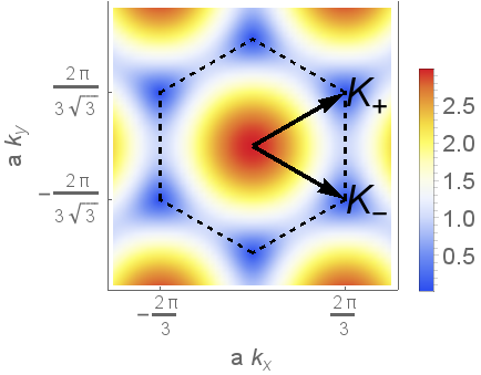
Figure 1: (Color Online) Brillouin zone with a density plot of $|\gamma(\vec{k})|$.

The geometry of the first Brillouin zone is visualized in Fig. 1 along with a color plot of the modulus $|\gamma(\vec{k})|$.

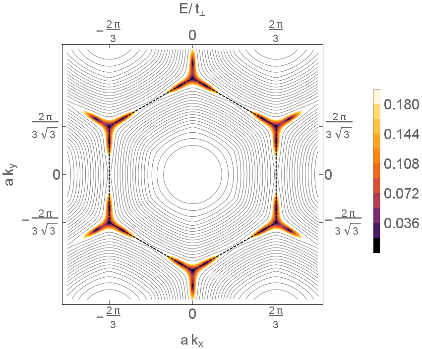
Figure 2: (Color Online) Contour plot of the energy band $(+E_{2}(\vec{k}))$ plotted for $t_{\perp}=t$, $t_{3}=0.5t$. The contour of the colored region indicates $E=0.2/t_{\perp}$. The edge of the first Brillouin zone is marked by dashed lines.

The presence of all four couplings in the Hamiltonian Eq. (2) makes its explicit diagonalization in terms of analytical expressions a particularly cumbersome task. As the present study chiefly relies on analytical calculations rather than resorts to numerics, we will drop the contributions proportional to the smallest parameter $t_{4}$ in order to achieve an analytically manageable situation.

Putting $t_{4}=0$ the full eigensystem of the Hamiltonian (2) can be obtained in a closed analytical fashion as detailed in appendix A. The four dispersion branches $(\pm E_{1}(\vec{k}))$, $(\pm E_{2}(\vec{k}))$ form a symmetric spectrum with

$$E_{1/2}=\sqrt{\frac{1}{2}\left(t_{\perp}^{2}+t_{3}^{2}|\gamma(\vec{k})|^{2}+2t^{2}|\gamma(\vec{k})|^{2}\pm\sqrt{4t^{2}|\gamma(\vec{k})|^{2}\left(t_{\perp}^{2}+t_{3}^{2}|\gamma(\vec{k})|^{2}-2t_{\perp}t_{3}|\gamma(\vec{k})|\cos\left(3\phi_{\vec{k}}\right)\right)+\left(t_{\perp}^{2}-t_{3}^{2}|\gamma(\vec{k})|^{2}\right)^{2}}\right)}$$ (5)

and $\gamma(\vec{k})=|\gamma(\vec{k})|e^{i\phi_{\vec{k}}}$. The two outer branches $(\pm E_{1}(\vec{k}))$ are separated from the inner ones $(\pm E_{2}(\vec{k}))$ by gaps determined essentially by the hopping parameter $t_{\perp}$. The result Eq. (5) generalizes the energy spectrum given in Ref. McCann06, within the Dirac cone approximation to the full Brillouin zone. Moreover, in appendix A we also give the complete data of the corresponding eigenvectors. Fig. 3 concentrates on the vicinity of a given $K$-point using realistic parameters.

The inner branches $(\pm E_{2}(\vec{k}))$ dominate the low-energy physics of the system near half filling and meet at zero energy for

$$\gamma(\vec{k})=0$$ (6)

corresponding to the two inequivalent corners $K_{\pm}$ of the first Brillouin zone, and for

$$\cos\left(3\phi_{\vec{k}}\right)=-1\quad\wedge\quad|\gamma(\vec{k})|=\frac{t_{\perp}t_{3}}{t^{2}}\,.$$ (7)

The latter condition defines three additional satellite Dirac cones around each $K$-point two of which lying on the edges (faces) of the Brillouin zone connecting $K_{\pm}$. The third satellite Dirac cone lies formally outside the Brillouin zone but is equivalent to a satellite cone on the edge around an equivalent $K$-point. Indeed, the quantity $\gamma(\vec{k})$ has a constant phase $\phi_{\vec{k}}\in\{-\pi/3,\pi/3,\pi\}$ on each face: As an example, consider the edge connecting the two inequivalent $K$-points given in Eq. (4) where one finds

$$\gamma\left(\frac{2\pi}{3a},k_{y}\right)=e^{-i\pi/3}\left(2\cos\left(\frac{\sqrt{3}}{2}k_{y}a\right)-1\right)$$ (8)

with the parenthesis being nonnegative for $k_{y}$ ranging between $(\pm 2\pi/(3\sqrt{3}a))$. Thus, solving for $k_{y}$ the satellite Dirac cones on that edge lie at

$$\vec{k}=\left(\frac{2\pi}{3a},\pm\frac{2}{\sqrt{3}a}\arccos\left(\frac{1}{2}\left(1+\frac{t_{\perp}t_{3}}{t^{2}}\right)\right)\right)\,,$$ (9)

and the other satellite cones are located at positions being equivalent under reciprocal lattice translation and/or hexagonal rotation. Note that for $t_{\perp}t_{3}/t^{2}=1$ the satellite cones merge in the $M$-points (centers of the faces) and they vanish for even larger values of that ratio. In Fig. 2 we give a sketch of the situation in the entire Brillouin zone for moderate values of $t_{\perp}$ and $t_{3}$.

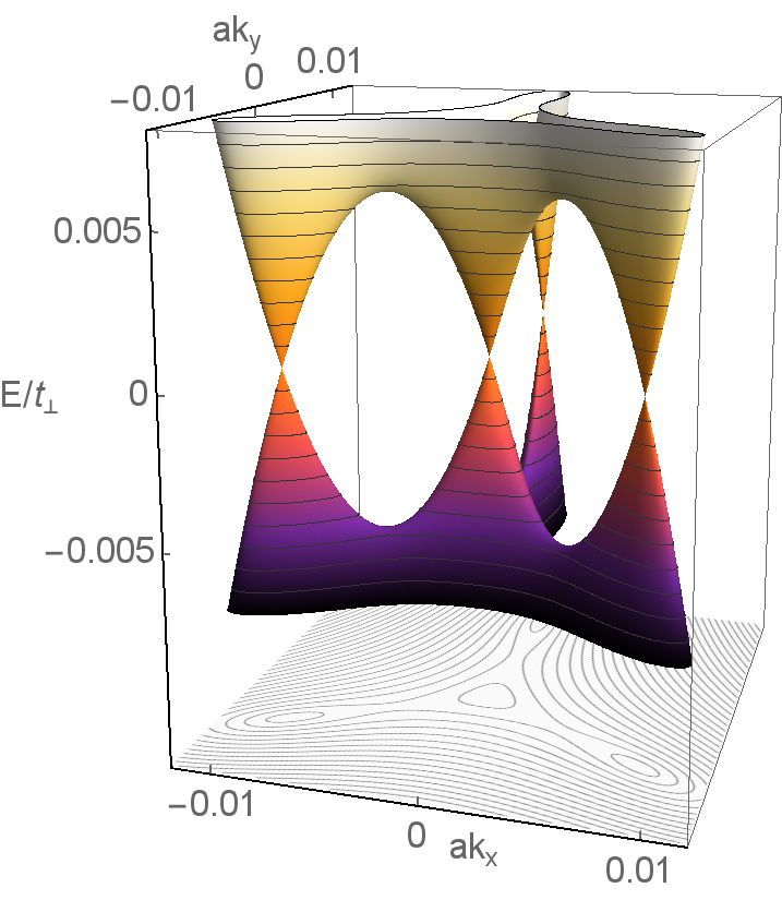
Figure 3: (Color Online) The central energy bands $(\pm E_{2}(\vec{k}))$ plotted around a given $K$-point for $t_{\perp}=0.1t$, $t_{3}=0.15t$. The dispersions show a central Dirac cone accompanied by three satellites. The components of the wave vector are measured relatively to the $K$-point.

For $t_{3}=0$ the two energy bands $(\pm E_{2}(\vec{k}))$ touch only at the $K$-points where they have a quadratic dispersion. Finite $t_{3}\neq 0$ causes a splitting into in total four Dirac cones with linear dispersion, an effect known as trigonal warping McCann13 ; Mariani12 .

As a further important property, the eigenvectors corresponding to $(\pm E_{2}(\vec{k}))$ are discontinuous as a function of wave vector at the degeneracy points defined by Eq. (7); for more technical details we refer to appendix B. As a simplistic toy model mimicking such an effect one can consider the Hamiltonian $H=-k\sigma^{z}$ with a one-dimensional wave number $k$ and the Pauli matrix $\sigma^{z}$ describing some internal degree of freedom: In the many-body ground state of zero Fermi energy all occupied states with $k>0$ have spin up while for all states with $k<0$ the spin points downwards, resulting in a discontinuity of the occupied eigenvectors at $k=0$. As we shall see below, in the present case of graphene bilayers this discontinuity is also reflected in the entanglement spectrum.

An effective Hamiltonian providing an approximate description of the central bands $(\pm E_{2}(\vec{k}))$ can be given following Ref. McCann06, . In up to linear order in $1/t_{\perp}$ one finds

$$H=-\left(\begin{array}[]{cc}0&\frac{t^{2}}{t_{\perp}}\left(\gamma^{\ast}(\vec{k})\right)^{2}+t_{3}\gamma(\vec{k})\\ \frac{t^{2}}{t_{\perp}}\left(\gamma(\vec{k})\right)^{2}+t_{3}\gamma^{\ast}(\vec{k})&0\end{array}\right)$$ (10)

with respect to the basis $\left(b_{2\vec{k}}^{\dagger},a_{1\vec{k}}^{\dagger}\right)|0\rangle$. The eigenstates read

$$|\chi_{\pm}\rangle=\frac{1}{\sqrt{2}}\left(\begin{array}[]{c}1\\ \mp e^{i\psi_{\vec{k}}}\end{array}\right)$$ (11)

with

$$e^{i\psi_{\vec{k}}}=\frac{\frac{t^{2}}{t_{\perp}}\left(\gamma(\vec{k})\right)^{2}+t_{3}\gamma^{\ast}(\vec{k})}{\left|\frac{t^{2}}{t_{\perp}}\left(\gamma(\vec{k})\right)^{2}+t_{3}\gamma^{\ast}(\vec{k})\right|}\,.$$ (12)

Note that the Hamiltonian (10) vanishes if and only if the conditions (6) or (7) are fulfilled implying that the positions of the central and satellite Dirac cones are the same as for the full Hamiltonian (2). Moreover , $\psi_{\vec{k}}$ is a smooth and well-defined function of the wave vector except for the locations of Dirac cones. Accordingly, the Berry curvature

$$F(\vec{k})=\frac{\partial A_{y}}{\partial k_{x}}-\frac{\partial A_{x}}{\partial k_{y}}$$ (13)

arising from the Berry connection

$$\vec{A}(\vec{k})=i\langle\chi_{\pm}(\vec{k})|\frac{\partial}{\partial\vec{k}}|\chi_{\pm}(\vec{k})\rangle=-\frac{1}{2}\frac{\partial\psi_{\vec{k}}}{\partial\vec{k}}$$ (14)

vanishes everywhere outside the Dirac cones where contributions in terms of $\delta$-functions arise. Integrating the Berry connection along closed path in $\vec{k}$-space leads to geometrical quantities often referred to as Berry phases, although no contact to adiabaticity is made here. Moreover, if the Berry curvature has only nonzero contributions in terms of $\delta$-functions (as it is the case here and in the following) these geometrical phases are indeed topological, i.e. they are invariant under continuous variations of the paths as long as the support of the $\delta$-functions is not touched.

As discussed in Refs. Manes07, ; Mikitik08, ; Mariani12, , integrating along a closed path around the central Dirac cones at $K_{\pm}$ yields a Berry phase of $(\mp\pi)$, while each of the accompanying satellite cones gives a contribution of $(\pm\pi)$. Thus, the total Berry phase arising at and around each $K$-point is, as in the absence of trigonal warping, $(\pm 2\pi)$, and the integral over the whole Brillouin zone of the Berry connection (i.e. the Chern number) vanishes. Naturally, our present analysis going beyond the Dirac cone approximation confirms these results.

III Entanglement Spectra

For systems of free fermions as studied here, the entanglement Hamiltonian can be formulated as a single-particle operator Peschel03 ; Cheong04 ; Schliemann13 ,

$$H_{\rm ent}=\sum_{\lambda}\xi_{\lambda}d^{\dagger}_{\lambda}d_{\lambda}\,.$$ (15)

Here the $d^{\dagger}_{\lambda}$ generate eigenstates of the correlation matrix

$$C_{\alpha\beta}=\langle\Psi|c_{\alpha}^{\dagger}c_{\beta}|\Psi\rangle\,,$$ (16)

where $|\Psi\rangle$ is the ground state of the composite system, and single-particle operators $c_{\alpha}$, $c_{\beta}$ act on its remaining part after tracing out a subsystem. The entanglement levels $\xi_{\lambda}$ are related to the eigenvalues $\eta_{\lambda}$ of the correlation matrix via

$$\xi_{\lambda}=\ln\left(\frac{1-\eta_{\lambda}}{\eta_{\lambda}}\right)={} 2\operatorname{artanh}\left(1-2\eta_{\lambda}\right)\,.$$ (17)

In particular, the entanglement Hamiltonian and the correlation matrix share the same system of eigenvectors.

III.1 Tracing out One Layer

We now consider the ground state of the undoped graphene bilayer such that all states with negative energies $(-E_{1}(\vec{k}))$, $(-E_{2}(\vec{k}))$ are occupied while all others are empty. Tracing out layer 1 leads to the correlation matrix

$$C(\vec{k})=\left(\begin{array}[]{cc}\frac{1}{2}&u(\vec{k})\\ u^{\ast}(\vec{k})&\frac{1}{2}\end{array}\right)$$ (18)

where an explicit expression for $u(\vec{k})$ is given in appendix C. The entanglement levels corresponding to the eigenvalues $\eta_{\pm}(\vec{k})=1/2\mp|u(\vec{k})|$ are

$$\xi_{\pm}(\vec{k})={} \pm 2\operatorname{artanh}\left(2|u(\vec{k})|\right)\,.$$ (19)

The modulus $|u|$ can be formulated as

$$|u|=\frac{1/2}{\sqrt{1+(d/(t|\gamma(\vec{k})|))^{2}}}\sqrt{\frac{1}{2}\left(1-\frac{\epsilon_{1}\epsilon_{2}+b^{2}}{E_{1}E_{2}}\right)}$$ (20)

with (cf. Eqs. (47),(48))

$$d = \frac{\left(t_{\perp}^{2}-t_{3}^{2}|\gamma(\vec{k})|^{2}\right)/2}{\sqrt{t_{\perp}^{2}+t_{3}^{2}|\gamma(\vec{k})|^{2}-2t_{\perp}t_{3}|\gamma(\vec{k})|\cos\left(3\phi_{\vec{k}}\right)}}\,,$$ (21)

$$b = \frac{t_{\perp}t_{3}|\gamma(\vec{k})||\sin\left(3\phi_{\vec{k}}\right)|}{\sqrt{t_{\perp}^{2}+t_{3}^{2}|\gamma(\vec{k})|^{2}-2t_{\perp}t_{3}|\gamma(\vec{k})|\cos\left(3\phi_{\vec{k}}\right)}}\,,$$ (22)

and (cf. Eq. (58))

$$\epsilon_{1,2}=t|\gamma(\vec{k})|$$

$$\pm\sqrt{\left(t_{\perp}^{2}+t_{3}^{2}|\gamma(\vec{k})|^{2}-2t_{\perp}t_{3}|\gamma(\vec{k})|\cos\left(3\phi_{\vec{k}}\right)\right)^{2}/4+d^{2}}$$

implying

$$E_{1,2}=\sqrt{\epsilon_{1,2}^{2}+b^{2}}\,.$$ (24)

The r.h.s of Eq. (20) becomes zero if the radicand vanishes. According to the discussion in appendices B and C this is the case when $\cos\left(3\phi_{\vec{k}}\right)=-1$ leading to $b=0$ and $E_{1}=\epsilon_{1}\geq 0$, $E_{2}=|\epsilon_{2}|$ such that

$$|u|\propto\sqrt{\frac{1}{2}\left(1-\frac{\epsilon_{2}}{|\epsilon_{2}|}\right)}$$ (25)

Now equation (81) shows that $|u(\vec{k})|=0$ is equivalent to

$$\cos\left(3\phi_{\vec{k}}\right)=-1\quad\wedge\quad|\gamma(\vec{k})|\in\left[0,t_{\perp}t_{3}/t^{2}\right]\,,$$ (26)

where the endpoint of the above interval defines according to condition (7) the location of the satellite Dirac cones. As a result, the entanglement levels (19) vanish along segments of the faces of the first Brillouin zone bounded by the positions of the central Dirac cones and their satellites. At the satellite Dirac cones the entanglement spectrum is discontinuous as a function of wave vector. In Fig. 4 we plotted the entanglement spectrum $\xi_{+}(\vec{k})$ for the whole Brillouin zone. For a better visualization large hopping parameters have been chosen. The contour of the colored region connects all three satellite Dirac cones. As discussed in appendix B, this discontinuity is inherited from a discontinuity in the eigenvectors of the occupied single-particle states. The entanglement spectrum in the entire Brillouin zone is illustrated in Fig. 4, whereas Fig. 5 focuses on a given $K$-point.

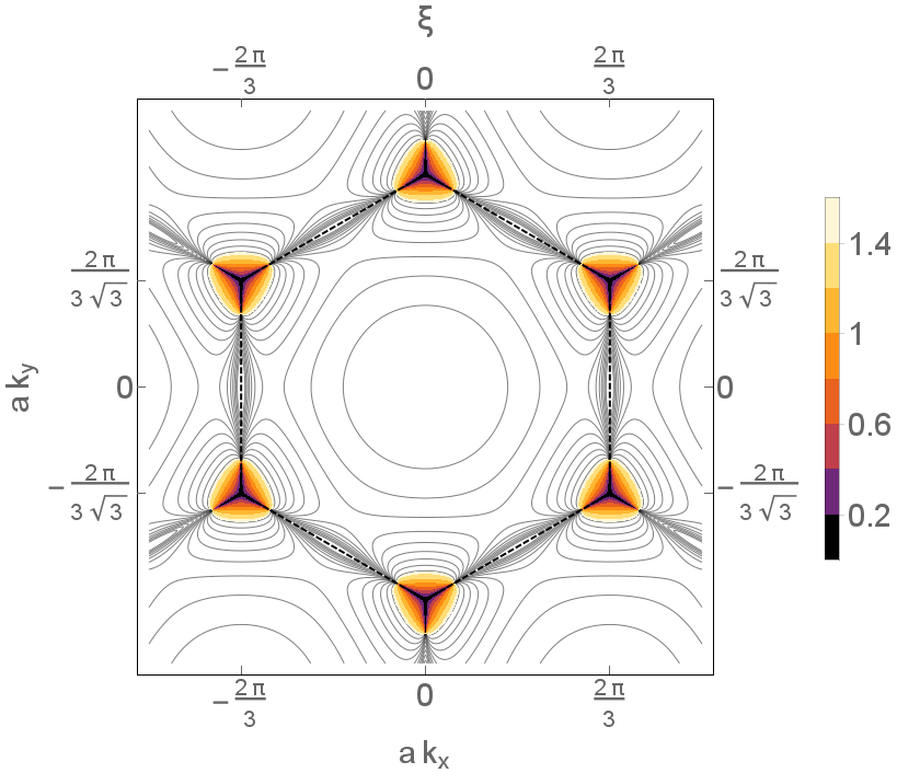
Figure 4: (Color Online) Contour plot of the entanglement spectrum $\xi_{+}(\vec{k})$ plotted for $t_{\perp}=t$, $t_{3}=0.5t$. The contour of the colored region indicates $\xi=1.5$. The dashed line delineates the first Brillouin zone.

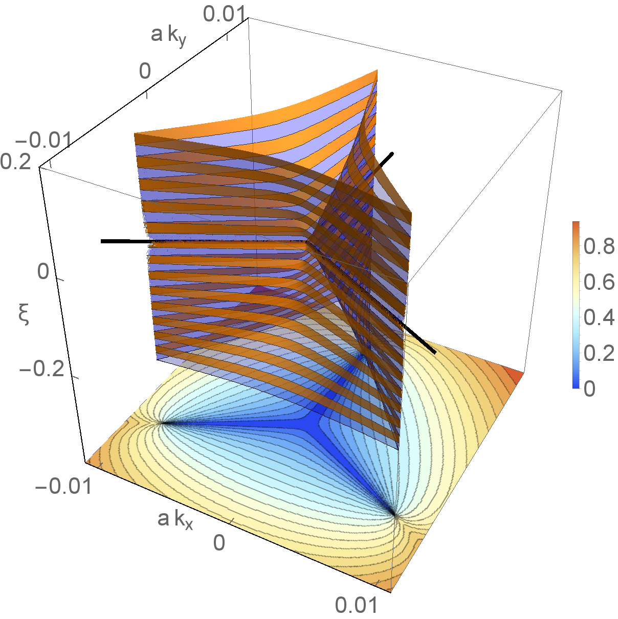
Figure 5: (Color Online) The entanglement spectrum (19) plotted around a given $K$-point for the same parameters as in Fig. 3. The density plot shows the upper entanglement level. Zero eigenvalues of the entanglement Hamiltonian occur along lines connecting the $K$-point with the locations of satellite Dirac cones of the energy spectrum (thick black lines). The components of the wave vector are measured relatively to the $K$-point.

Moreover, apart from the eigenvalues of the entanglement Hamiltonian, let us also consider its eigenvector which coincide with the eigenvectors of the correlation matrix (18). As discussed in appendix C, the complex function $u(\vec{k})$ entering the correlation matrix becomes singular at the $K$-points and the positions of the accompanying satellite Dirac cones of the energy spectrum, leading again to $\delta$-function-type contributions to the Berry curvature which vanishes otherwise. Combining symbolic computer algebra techniques and numerical calculations we find here a Berry phase of $(\mp\pi/2)$ around the corners $K_{\pm}$ of the Brillouin zone, and $(\pm\pi/2)$ for the corresponding satellite positions. For the central positions the above calculations can also be done fully analytically by expanding the eigensystem data around $K_{\pm}$. For the satellite locations such an expansion is not possible due to the discontinuity of the eigenvectors.

Thus, the total Berry phase contribution from each $K$-point $K_{\pm}$ is $(\pm\pi)$ and agrees with the Berry phase around the Dirac cones in monolayer graphene. As a result, although the entanglement spectrum of graphene bilayers generated by tracing out one layer shows obvious differences to the energy spectrum of monolayer graphene regarding qualitative geometrical properties, the topological Berry phases obtained from the corresponding eigenvectors still coincide at each $K$-point.

III.2 Tracing out other Sublattices

Now, we will consider the entanglement spectrum obtained by tracing out sublattices A1 and B2 (or A2 and B1) lying in different layers. In the former case one finds

$$C(\vec{k})=\left(\begin{array}[]{cc}\frac{1}{2}&v(\vec{k})\\ v^{\ast}(\vec{k})&\frac{1}{2}\end{array}\right)$$ (27)

where an explicit expression for $v(\vec{k})$ is given in appendix C. The above correlation matrix has eigenvalues $\eta_{\pm}(\vec{k})=1/2\mp|v(\vec{k})|$ leading to the entanglement levels

$$\xi_{\pm}(\vec{k})={} \pm 2\operatorname{artanh}\left(2|v(\vec{k})|\right)\,.$$ (28)

In Fig. 6 we plotted the eigenvalues $\eta_{-}(\vec{k})=1/2+|v(\vec{k})|$ of the correlation matrix around a given $K$-point. The modulus $|v(\vec{k})|$ reads more explicitly

$$|v(\vec{k})|={} \frac{1}{2}\sqrt{1-\frac{t^{2}|\gamma(\vec{k})|^{2}}{t^{2}|\gamma(\vec{k})|^{2}+d^{2}}\frac{1}{2}\left(1-\frac{\epsilon_{1}\epsilon_{2}+b^{2}}{E_{1}E_{2}}\right)}$$ (29)

$$={} \frac{1}{2}\sqrt{1-4|u(\vec{k})|^{2}}$$ (30)

and has a similar structure as $|u(\vec{k})|$ given in Eq. (20). In particular, $|v(\vec{k})|=1/2\Leftrightarrow|u(\vec{k})|=0$ if the conditions (26) are fulfilled. In this case $\eta_{+}=0$ and $\eta_{-}=1$ indicating that the remaining subsystem is unentangled with the system traced out.

Regarding Berry phases generated from the eigenstates of the correlation matrix (27) we note that the off-diagonal element $v(\vec{k})$ nowhere vanishes. As a consequence the Berry curvature defined analogously as in Eqs. (11)-(14) is zero throughout the Brillouin zone, which in turn holds for all Berry phases. The nonvanishing of $v(\vec{k})$ follows from the fact that $|v(\vec{k})|=0$ would require $|u(\vec{k})|=1/2$ such that the entanglement (19) would diverge which is, as seen in section III.1, not the case.

Finally, the correlation matrix obtained by tracing over the sublattices A1, A2 (or B1, B2) is proportional to the unit matrix,

$$C(\vec{k})={} \left(\begin{array}[]{cc}\frac{1}{2}&0\\ 0&\frac{1}{2}\end{array}\right),$$ (33)

indicating that these sublattices are maximally entangled with the part traced out.

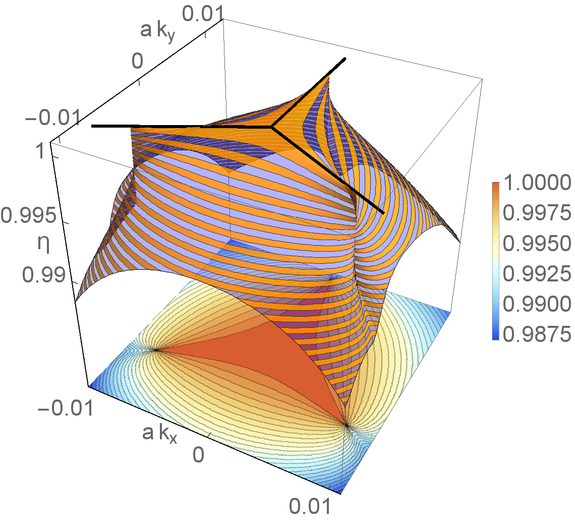
Figure 6: (Color Online) Eigenvalues $\eta_{-}(\vec{k})=1/2+|v(\vec{k})|$ of the correlation matrix plotted around a given $K$-point for $t_{\perp}=0.1t$, $t_{3}=0.15t$. The thick black lines correspond to the one in Fig. 5, and the components of the wave vector are again measured relatively to the $K$-point.

IV Conclusions and Outlook

We have studied entanglement properties of the ground state of Bernal stacked graphene bilayers in the presence of trigonal warping. Our analysis includes both the eigenvalues of the reduced density matrix (giving rise to the entanglement spectrum) as well as its eigenvectors. When tracing out one layer, the entanglement spectrum shows qualitative geometric differences to the energy spectrum of a graphene monolayer while topological quantities such as Berry phase type contributions to Chern numbers agree. The latter finding is in contrast to the reduced density matrix resulting from tracing out other sublattices of the bilayer system. Here, all corresponding Berry phase integrals yield trivially zero. Thus, our study provides an example for common topological properties of the eigensystem of the energy Hamiltonian of a subsystem (here a graphene monolayer) and the entanglement Hamiltonian, while the geometrical shape of both spectra grossly differs. Our investigations are based on closed analytical expressions for the full eigensystem of bilayer graphene in the entire Brillouin zone with a trigonally warped spectrum.

Future work might address bilayer systems of other geometrical structures such as the Kagome lattice, the influence of a static perpendicular magnetic field Nemec07 ; Schliemann13 , and the effect of time-periodic in-plane electric fields Wang15 .

Note added. After this paper was made available as an arXiv preprint and submitted to the journal, we became aware of Ref. Fukui14 where also Chern numbers calculated from the eigenstates of entanglement Hamiltonians are studied. Most recent work building upon this concept is reported on in Ref. Araki16 .

Appendix A Diagonalization of the Bilayer Hamiltonian

Putting $t_{4}=0$ and fixing a wave vector $\vec{k}$ the Hamiltonian (2) reads with respect to the basis $\left(a_{2\vec{k}}^{\dagger},b_{1\vec{k}}^{\dagger},b_{2\vec{k}}^{\dagger},a_{1\vec{k}}^{\dagger}\right)|0\rangle$

$$H=\left(\begin{array}[]{cccc}0&t_{\perp}&-t\gamma(\vec{k})&0\\ t_{\perp}&0&0&-t\gamma^{\ast}(\vec{k})\\ -t\gamma^{\ast}(\vec{k})&0&0&-t_{3}\gamma(\vec{k})\\ 0&-t\gamma(\vec{k})&-t_{3}\gamma^{*}(\vec{k})&0\\ \end{array}\right)\,.$$ (34)

Using $\gamma(\vec{k})=|\gamma(\vec{k})|e^{i\phi_{\vec{k}}}$ we apply the transformation

$$U_{1}=\frac{1}{\sqrt{2}}\left(\begin{array}[]{cccc}1&1&0&0\\ 0&0&e^{i\phi_{\vec{k}}}&e^{-i\phi_{\vec{k}}}\\ 0&0&e^{i\phi_{\vec{k}}}&-e^{-i\phi_{\vec{k}}}\\ 1&-1&0&0\\ \end{array}\right)$$ (35)

such that in

$$H_{1}=U_{1}HU_{1}^{\dagger}=\left(\begin{array}[]{cccc}t_{\perp}&-t|\gamma(\vec{k})|&0&0\\ -t|\gamma(\vec{k})|&-t_{3}|\gamma(\vec{k})|\cos\left(3\phi_{\vec{k}}\right)&it_{3}|\gamma(\vec{k})|\sin\left(3\phi_{\vec{k}}\right)&0\\ 0&-it_{3}|\gamma(\vec{k})|\sin\left(3\phi_{\vec{k}}\right)&t_{3}|\gamma(\vec{k})|\cos\left(3\phi_{\vec{k}}\right)&-t|\gamma(\vec{k})|\\ 0&0&-t|\gamma(\vec{k})|&-t_{\perp}\end{array}\right)$$ (36)

all information on the phase $\phi_{\vec{k}}$ is contained in the matrix elements being proportional to the skew parameter $t_{3}$. Proceeding now with the transformation

$$U_{2}=\frac{1}{\sqrt{2}}\left(\begin{array}[]{cccc}1&-1&0&0\\ 1&1&0&0\\ 0&0&1&-1\\ 0&0&1&1\end{array}\right)$$ (37)

we find

$$H_{2}=U_{2}H_{1}U_{2}^{\dagger}=\frac{1}{2}\left(\begin{array}[]{cccc}e_{1}&c&-is&-is\\ c&e_{2}&is&is\\ is&-is&-e_{2}&c\\ is&-is&c&-e_{1}\end{array}\right)$$ (38)

with

$$e_{1} = \phantom{-}2t|\gamma(\vec{k})|+t_{\perp}-t_{3}|\gamma(\vec{k})|\cos\left(3\phi_{\vec{k}}\right)\,,$$ (39)

$$e_{2} = -2t|\gamma(\vec{k})|+t_{\perp}-t_{3}|\gamma(\vec{k})|\cos\left(3\phi_{\vec{k}}\right)\,,$$ (40)

$$c = t_{\perp}+t_{3}|\gamma(\vec{k})|\cos\left(3\phi_{\vec{k}}\right)\,,$$ (41)

$$s = t_{3}|\gamma(\vec{k})|\sin\left(3\phi_{\vec{k}}\right)\,.$$ (42)

Here it is useful to split the above matrix as $H_{2}=H_{2}^{{}^{\prime}}+H_{2}^{{}^{\prime\prime}}$ where

$$H_{2}^{{}^{\prime}}=\frac{1}{2}\left(\begin{array}[]{cccc}e_{1}&0&-is&0\\ 0&e_{2}&0&is\\ is&0&-e_{2}&0\\ 0&-is&0&-e_{1}\end{array}\right)\quad,\quad H_{2}^{{}^{\prime\prime}}=\frac{1}{2}\left(\begin{array}[]{cccc}0&c&0&-is\\ c&0&is&0\\ 0&-is&0&c\\ is&0&c&0\end{array}\right)\,.$$ (43)

$H_{2}^{{}^{\prime}}$ is diagonalized by

$$U_{3}=\left(\begin{array}[]{cccc}\alpha_{+}&0&-i\sigma\alpha_{-}&0\\ 0&-i\sigma\alpha_{+}&0&\alpha_{-}\\ -i\sigma\alpha_{-}&0&\alpha_{+}&0\\ 0&\alpha_{-}&0&-i\sigma\alpha_{+}\end{array}\right)$$ (44)

with $\sigma=\operatorname{sign}\left(\sin(3\phi(\vec{k}))\right)$ and

$$\alpha_{\pm}={} \sqrt{\frac{1}{2}\left(1\pm\frac{t_{\perp}-t_{3}|\gamma(\vec{k})|\cos\left(3\phi_{\vec{k}}\right)}{\sqrt{t_{\perp}^{2}+t_{3}^{2}|\gamma(\vec{k})|^{2}-2t_{\perp}t_{3}|\gamma(\vec{k})|\cos\left(3\phi_{\vec{k}}\right)}}\right)}$$ (45)

such that

$$H_{3}=U_{3}H_{2}U_{3}^{\dagger}=\left(\begin{array}[]{cccc}\zeta_{1}&id\sigma&0&b\\ -id\sigma&\zeta_{2}&b&0\\ 0&b&-\zeta_{2}&id\sigma\\ b&0&-id\sigma&-\zeta_{1}\end{array}\right)$$ (46)

where

$$d = \frac{\left(t_{\perp}^{2}-t_{3}^{2}|\gamma(\vec{k})|^{2}\right)/2}{\sqrt{t_{\perp}^{2}+t_{3}^{2}|\gamma(\vec{k})|^{2}-2t_{\perp}t_{3}|\gamma(\vec{k})|\cos\left(3\phi_{\vec{k}}\right)}}\,,$$ (47)

$$b = \frac{t_{\perp}t_{3}|\gamma(\vec{k})||\sin\left(3\phi_{\vec{k}}\right)|}{\sqrt{t_{\perp}^{2}+t_{3}^{2}|\gamma(\vec{k})|^{2}-2t_{\perp}t_{3}|\gamma(\vec{k})|\cos\left(3\phi_{\vec{k}}\right)}}\,,$$ (48)

and $\pm\zeta_{1}$ and $\pm\zeta_{2}$ are eigenvalues of $H_{2}^{{}^{\prime}}$ given by

$$\zeta_{1/2}=\frac{1}{2}\left(\pm 2t|\gamma(\vec{k})|+\sqrt{t_{\perp}^{2}+t_{3}^{2}|\gamma(\vec{k})|^{2}-2t_{\perp}t_{3}|\gamma(\vec{k})|\cos\left(3\phi_{\vec{k}}\right)}\right)\,.$$ (49)

Splitting now $H_{3}$ in the form

$$H_{3}=\left(\begin{array}[]{cccc}\zeta_{1}&id&0&0\\ -id&\zeta_{2}&0&0\\ 0&0&-\zeta_{2}&id\\ 0&0&-id&-\zeta_{1}\end{array}\right)+\left(\begin{array}[]{cccc}0&0&0&b\\ 0&0&b&0\\ 0&b&0&0\\ b&0&0&0\end{array}\right)$$ (50)

the first part is diagonalized by

$$U_{4}=\left(\begin{array}[]{cccc}-i\sigma\tau\beta_{+}&\beta_{-}&0&0\\ \beta_{-}&-i\sigma\tau\beta_{+}&0&0\\ 0&0&-i\sigma\tau\beta_{+}&\beta_{-}\\ 0&0&\beta_{-}&-i\sigma\tau\beta_{+}\end{array}\right)$$ (55)

with $\tau=\operatorname{sign}(d)$ and

$$\beta_{\pm}=\sqrt{\frac{1}{2}\left(1\pm\frac{\zeta_{1}-\zeta_{2}}{\sqrt{(\zeta_{1}-\zeta_{2})^{2}+4d^{2}}}\right)}$$ (56)

while the second part is left unchanged by $U_{4}$ resulting in

$$H_{4}=U_{4}H_{3}U_{4}^{\dagger}=\left(\begin{array}[]{cccc}\epsilon_{1}&0&0&b\\ 0&\epsilon_{2}&b&0\\ 0&b&-\epsilon_{2}&0\\ b&0&0&-\epsilon_{1}\end{array}\right)$$ (57)

with the diagonal elements are given in terms of

$$\epsilon_{1/2}=\frac{1}{2}\left(\zeta_{1}+\zeta_{2}\pm\sqrt{\left(\zeta_{1}-\zeta_{2}\right)^{2}+4d^{2}}\right)\,.$$ (58)

Finally, $H_{4}$ is brought into diagonal form via

$$U_{5}=\left(\begin{array}[]{cccc}\gamma_{+}^{(1)}&0&0&\gamma_{-}^{(1)}\\ 0&\gamma_{+}^{(2)}&\gamma_{-}^{(2)}&0\\ 0&\gamma_{-}^{(2)}&-\gamma_{+}^{(2)}&0\\ \gamma_{-}^{(1)}&0&0&-\gamma_{+}^{(1)}\end{array}\right)$$ (59)

with

$$\gamma_{\pm}^{(1)}=\sqrt{\frac{1}{2}\left(1\pm\frac{\epsilon_{1}}{E_{2}}\right)}\quad,\quad\gamma_{\pm}^{(2)}=\sqrt{\frac{1}{2}\left(1\pm\frac{\epsilon_{2}}{E_{2}}\right)}$$ (60)

and

$$E_{1/2}=\sqrt{\epsilon_{1,2}^{2}+b^{2}}$$ (61)

$$=\sqrt{\frac{1}{2}\left(t_{\perp}^{2}+t_{3}^{2}|\gamma(\vec{k})|^{2}+2t^{2}|\gamma(\vec{k})|^{2}\pm\sqrt{4t^{2}|\gamma(\vec{k})|^{2}\left(t_{\perp}^{2}+t_{3}^{2}|\gamma(\vec{k})|^{2}-2t_{\perp}t_{3}|\gamma(\vec{k})|\cos\left(3\phi_{\vec{k}}\right)\right)+\left(t_{\perp}^{2}-t_{3}^{2}|\gamma(\vec{k})|^{2}\right)^{2}}\right)}.$$

Thus,

$$U_{5}H_{4}U_{5}^{\dagger}={} \operatorname{diag}\left(E_{1},E_{2},-E_{2},-E_{1}\right)\,,$$ (63)

and the matrix elements of the corresponding total transformation $U=U_{5}U_{4}U_{3}U_{2}U_{1}$ can be expressed as

$$U_{11} = \frac{1}{2}\left(\alpha_{-}-i\sigma\alpha_{+}\right)\left(\tau\beta_{+}+\beta_{-}\right)\left(\gamma_{+}^{(1)}-i\sigma\gamma_{-}^{(1)}\right)$$ (64)

$$U_{12} = \frac{1}{2}\left(\alpha_{+}-i\sigma\alpha_{-}\right)\left(\tau\beta_{+}+\beta_{-}\right)\left(\gamma_{-}^{(1)}-i\sigma\gamma_{+}^{(1)}\right)$$ (65)

$$U_{13} = -\frac{e^{i\phi_{\vec{k}}}}{2}\left(\alpha_{-}-i\sigma\alpha_{+}\right)\left(\tau\beta_{+}-\beta_{-}\right)\left(\gamma_{+}^{(1)}+i\sigma\gamma_{-}^{(1)}\right)$$ (66)

$$U_{14} = \frac{e^{-i\phi_{\vec{k}}}}{2}\left(\alpha_{-}+i\sigma\alpha_{+}\right)\left(\tau\beta_{+}-\beta_{-}\right)\left(\gamma_{+}^{(1)}-i\sigma\gamma_{-}^{(1)}\right)$$ (67)

and

$$U_{21} = -\frac{1}{2}\left(\alpha_{+}+i\sigma\alpha_{-}\right)\left(\tau\beta_{+}-\beta_{-}\right)\left(\gamma_{+}^{(2)}-i\sigma\gamma_{-}^{(2)}\right)$$ (68)

$$U_{22} = -\frac{1}{2}\left(\alpha_{+}-i\sigma\alpha_{-}\right)\left(\tau\beta_{+}-\beta_{-}\right)\left(\gamma_{+}^{(2)}+i\sigma\gamma_{-}^{(2)}\right)$$ (69)

$$U_{23} = -\frac{e^{i\phi_{\vec{k}}}}{2}\left(\alpha_{+}+i\sigma\alpha_{-}\right)\left(\tau\beta_{+}+\beta_{-}\right)\left(\gamma_{+}^{(2)}+i\sigma\gamma_{-}^{(2)}\right)$$ (70)

$$U_{24} = -\frac{e^{-i\phi_{\vec{k}}}}{2}\left(\alpha_{+}-i\sigma\alpha_{-}\right)\left(\tau\beta_{+}+\beta_{-}\right)\left(\gamma_{+}^{(2)}-i\sigma\gamma_{-}^{(2)}\right)$$ (71)

which are the complex conjugates of the components of the eigenvectors of the conduction-band states with positive energies $E_{1}(\vec{k})$, $E_{2}(\vec{k})$, while

$$U_{31} = \frac{1}{2}\left(\alpha_{-}-i\sigma\alpha_{+}\right)\left(\tau\beta_{+}-\beta_{-}\right)\left(\gamma_{+}^{(2)}-i\sigma\gamma_{-}^{(2)}\right)$$ (72)

$$U_{32} = \frac{1}{2}\left(\alpha_{-}+i\sigma\alpha_{+}\right)\left(\tau\beta_{+}-\beta_{-}\right)\left(\gamma_{+}^{(2)}+i\sigma\gamma_{-}^{(2)}\right)$$ (73)

$$U_{33} = -\frac{e^{i\phi_{\vec{k}}}}{2}\left(\alpha_{+}+i\sigma\alpha_{-}\right)\left(\tau\beta_{+}+\beta_{-}\right)\left(\gamma_{-}^{(2)}-i\sigma\gamma_{+}^{(2)}\right)$$ (74)

$$U_{34} = -\frac{e^{-i\phi_{\vec{k}}}}{2}\left(\alpha_{+}-i\sigma\alpha_{-}\right)\left(\tau\beta_{+}+\beta_{-}\right)\left(\gamma_{-}^{(2)}+i\sigma\gamma_{+}^{(2)}\right)$$ (75)

and

$$U_{41} = \phantom{-}\frac{1}{2}\left(\alpha_{+}+i\sigma\alpha_{-}\right)\left(\tau\beta_{+}+\beta_{-}\right)\left(\gamma_{+}^{(1)}-i\sigma\gamma_{-}^{(1)}\right)$$ (76)

$$U_{42} = -\frac{1}{2}\left(\alpha_{-}+i\sigma\alpha_{+}\right)\left(\tau\beta_{+}+\beta_{-}\right)\left(\gamma_{-}^{(1)}-i\sigma\gamma_{+}^{(1)}\right)$$ (77)

$$U_{43} = \frac{e^{i\phi_{\vec{k}}}}{2}\left(\alpha_{+}+i\sigma\alpha_{-}\right)\left(\tau\beta_{+}-\beta_{-}\right)\left(\gamma_{+}^{(1)}+i\sigma\gamma_{-}^{(1)}\right)$$ (78)

$$U_{44} = \frac{e^{-i\phi_{\vec{k}}}}{2}\left(\alpha_{-}+i\sigma\alpha_{+}\right)\left(\tau\beta_{+}-\beta_{-}\right)\left(\gamma_{-}^{(1)}+i\sigma\gamma_{+}^{(1)}\right)$$ (79)

correspond to the valence-band states with negative energies $(-E_{2}(\vec{k}))$, $(-E_{1}(\vec{k}))$. Note that all factors involving $\alpha_{\pm}$, $\gamma_{\pm}^{(1)}$, $\gamma_{\pm}^{(2)}$ in the above expressions have modulus one, i.e. they are phase factors.

Appendix B Continuity Properties

The eigenvectors corresponding to the energy branches $(\pm E_{2}(\vec{k}))$ are discontinuous at wave vectors determined by the condition (7). This comes about as follows: The matrix elements $U_{2,n}(\vec{k})$, $U_{3,n}(\vec{k})$, $n\in\{1,2,3,4\}$ contain the quantities $\gamma_{\pm}^{(2)}$ defined in Eqs. (60) whereas the $U_{1,n}(\vec{k})$, $U_{4,n}(\vec{k})$ corresponding to $(\pm E_{1}(\vec{k}))$ involve $\gamma_{\pm}^{(1)}$ Fixing now $\cos\left(\phi_{\vec{k}}\right)=-1$ we have $b=0$ such that $E_{1}=\epsilon_{1}\geq 0$ and $E_{2}=|\epsilon_{2}|$ such that $\gamma_{\pm}^{(1)}$ remain continuous while $\gamma_{\pm}^{(2)}$ become

$$\gamma_{\pm}^{(2)}=\sqrt{\frac{1}{2}\left(1\pm\frac{\epsilon_{2}}{|\epsilon_{2}|}\right)}\,.$$ (80)

Inspection of Eq. (58) now shows that for $\cos\left(\phi_{\vec{k}}\right)=-1$

$$\epsilon_{2}(\vec{k})\left\{\begin{array}[]{cc}>0&\,|\gamma(\vec{k})|<t_{\perp}t_{3}/t^{2}\\ <0&\,|\gamma(\vec{k})|>t_{\perp}t_{3}/t^{2}\end{array}\right.$$ (81)

such that $\epsilon_{2}(\vec{k})$ changes sign for $|\gamma(\vec{k})|=t_{\perp}t_{3}/t^{2}$, i.e. $\gamma_{\pm}^{(2)}$ is discontinuous at wave vectors given by the condition (7). This discontinuity is inherited by the correlation matrix and, in turn, by the entanglement spectrum.

The technical reason for this discontinuity in the eigenvectors is of course the fact that the dispersions $(\pm E_{2}(\vec{k}))$ become degenerate at wave vectors fulfilling (7). In fact the eigenvectors can also be considered as continuous functions of the wave vector by appropriately relabeling the dispersion branches. In the ground state of the undoped bilayer system, however, only the lower branch $(-E_{2}(\vec{k}))$ is occupied, which makes the discontinuity unavoidable.

To circumvent this discontinuity one can open an energy gap between the upper and lower central band such that the corresponding eigenstates are necessarily continuous for all wave vectors. Among the various mechanisms producing such a gap only few allow for a still halfway convenient analytical treatment of the Hamiltonian. These include introducing identical mass terms in both layers, i.e. $H\mapsto H+H^{\prime}$ with

$$H^{\prime}={} \operatorname{diag}\left(m,-m,-m,m\right)\,,$$ (82)

or applying a bias voltage $\Lambda$ between the layers,

$$H^{\prime}={} \operatorname{diag}\left(-\Lambda/2,\Lambda/2,-\Lambda/2,\Lambda/2\right)\,.$$ (83)

In the former case the four dispersion branches $(\pm E_{1}(\vec{k}))$, $(\pm E_{2}(\vec{k}))$ are given by

$$E_{1/2}(\vec{k}) = \Biggl{[}m^{2}+\frac{1}{2}\left(t_{\perp}^{2}+t_{3}^{2}|\gamma(\vec{k})|^{2}+2t^{2}|\gamma(\vec{k})|^{2}\right)$$ (84)

$$\pm\frac{1}{2}\sqrt{4t^{2}|\gamma(\vec{k})|^{2}\left(t_{\perp}^{2}+t_{3}^{2}|\gamma(\vec{k})|^{2}-2t_{\perp}t_{3}|\gamma(\vec{k})|\cos\left(3\phi_{\vec{k}}\right)\right)+\left(t_{\perp}^{2}-t_{3}^{2}|\gamma(\vec{k})|^{2}\right)^{2}}\Biggr{]}^{1/2}$$

while for a bias voltage one finds McCann06

$$E_{1/2}(\vec{k}) = \Biggl{[}\frac{\Lambda^{2}}{4}+\frac{1}{2}\left(t_{\perp}^{2}+t_{3}^{2}|\gamma(\vec{k})|^{2}+2t^{2}|\gamma(\vec{k})|^{2}\right)$$ (85)

$$\pm\frac{1}{2}\sqrt{4t^{2}|\gamma(\vec{k})|^{2}\left(t_{\perp}^{2}+t_{3}^{2}|\gamma(\vec{k})|^{2}-2t_{\perp}t_{3}|\gamma(\vec{k})|\cos\left(3\phi_{\vec{k}}\right)+\Lambda^{2}\right)+\left(t_{\perp}^{2}-t_{3}^{2}|\gamma(\vec{k})|^{2}\right)^{2}}\Biggr{]}^{1/2}\,.$$

In both cases the central energy bands $(\pm E_{2}(\vec{k}))$ are separated by a gap, and the spectrum can still be given in terms of comparably simple closed expressions since the characteristic polynomial of the $4\times 4$ Hamiltonian matrix is a second-order polynomial in the energy squared leading to a spectrum being symmetric around zero. Also the corresponding eigenvectors can be obtained in closed analytical forms by procedures analogous to (but in detail somewhat more complicated than) the one given in appendix A Predin15 .

Note that applying a bias voltage as well as introducing a mass term in each layer discriminates the layers against each other. The latter circumstance is due to the fact that $t_{\perp}$ couples sublattices in different layers for which the mass term has different sign. As a result, when tracing out, say, one layer of an undoped (i.e. half-filled) bilayer system, the remaining layer will not be half-filled, what obscures somewhat the comparison with an undoped graphene monolayer.

Appendix C Correlation Matrices

Upon tracing out layer $1$ from the ground state of the undoped bilayer system the correlation matrix reads in the basis $\left(a_{2\vec{k}}^{\dagger},b_{2\vec{k}}^{\dagger}\right)|0\rangle$

$$C(\vec{k})=\left(\begin{array}[]{cc}U_{31}U_{31}^{\ast}+U_{41}U_{41}^{\ast}&U_{31}U_{33}^{\ast}+U_{41}U_{43}^{\ast}\\ U_{33}U_{31}^{\ast}+U_{43}U_{41}^{\ast}&U_{33}U_{33}^{\ast}+U_{43}U_{43}^{\ast}\end{array}\right)=\left(\begin{array}[]{cc}\frac{1}{2}&u(\vec{k})\\ u^{\ast}(\vec{k})&\frac{1}{2}\end{array}\right)$$ (86)

with

$$u(\vec{k})=\frac{e^{-i\phi_{\vec{k}}}}{4}\left(\beta_{+}^{2}-\beta_{-}^{2}\right)\left(\left(\gamma_{+}^{(1)}-i\sigma\gamma_{-}^{(1)}\right)^{2}-\left(\gamma_{+}^{(2)}-i\sigma\gamma_{-}^{(2)}\right)^{2}\right)\,.$$ (87)

This quantity becomes singular at the corners of the Brillouin zone where $\gamma(\vec{k})$ is zero such that its phase is ill-defined, and at the positions of the satellite Dirac cones of the energy spectrum where, as discussed in appendix B, $\gamma_{\pm}^{(2)}$ is discontinuous.

Tracing out the sublattices A1 and B2 one finds in the basis $\left(a_{2\vec{k}}^{\dagger},b_{1\vec{k}}^{\dagger}\right)|0\rangle$

$$C(\vec{k})=\left(\begin{array}[]{cc}U_{31}U_{31}^{\ast}+U_{41}U_{41}^{\ast}&U_{31}U_{32}^{\ast}+U_{41}U_{42}^{\ast}\\ U_{32}U_{31}^{\ast}+U_{42}U_{41}^{\ast}&U_{32}U_{32}^{\ast}+U_{42}U_{42}^{\ast}\end{array}\right)=\left(\begin{array}[]{cc}\frac{1}{2}&v(\vec{k})\\ v^{\ast}(\vec{k})&\frac{1}{2}\end{array}\right)$$ (88)

with

$$v(\vec{k})=\frac{\left(\alpha_{-}-i\sigma\alpha_{+}\right)^{2}}{4}\left(\left(\tau\beta_{+}-\beta_{-}\right)^{2}\left(\gamma_{+}^{(2)}-i\sigma\gamma_{-}^{(2)}\right)^{2}+\left(\tau\beta_{+}+\beta_{-}\right)^{2}\left(\gamma_{+}^{(1)}-i\sigma\gamma_{-}^{(1)}\right)^{2}\right)\,.$$ (89)

Note that the expressions (87),(89) obey the interesting sum rule

$$|u(\vec{k})|^{2}+|v(\vec{k})|^{2}=\frac{1}{4}$$ (90)

which s fulfilled whenever the coefficients involved satisfy

$$\alpha_{+}^{2}+\alpha_{-}^{2}=\beta_{+}^{2}+\beta_{-}^{2}=\left(\gamma_{+}^{(1/2)}\right)^{2}+\left(\gamma_{-}^{(1/2)}\right)^{2}=1\,,$$ (91)

which is the case here by construction.

Finally, the correlation matrix obtained by tracing out the sublattices A1, A2 is proportional to the unit matrix,

$$C(\vec{k})=\left(\begin{array}[]{cc}U_{32}U_{32}^{\ast}+U_{42}U_{42}^{\ast}&U_{32}U_{33}^{\ast}+U_{42}U_{43}^{\ast}\\ U_{33}U_{32}^{\ast}+U_{43}U_{42}^{\ast}&U_{33}U_{33}^{\ast}+U_{43}U_{43}^{\ast}\end{array}\right)=\left(\begin{array}[]{cc}\frac{1}{2}&0\\ 0&\frac{1}{2}\end{array}\right)$$ (92)

implying that the remaining subsystem is maximally entangled with the subsystem traced out.

References

- (1) L. Bombelli, R. K. Koul, J. Lee, and R. D. Sorkin, Phys. Rev. D 34, 373 (1986).
- (2) J. Eisert, M. Cramer, and M. B. Plenio, Rev. Mod. Phys. 82, 277 (2010).
- (3) H. Li and F. D. M. Haldane, Phys. Rev. Lett. 101, 010504 (2008).
- (4) A. M. Läuchli, E. J. Bergholtz, J. Suorsa, and M. Haque, Phys. Rev. Lett. 104, 156404 (2010).
- (5) R. Thomale, D. P. Arovas, B. A. Bernevig, Phys. Rev. Lett 105, 116805 (2010).
- (6) A. Chandran, M. Hermanns, N. Regnault, and B. A. Bernevig, Phys. Rev. B 84, 205136 (2011).
- (7) A. Kitaev, Ann. Phys. 321, 2 (2006).
- (8) A. M. Turner, Y. Zhang, A. Vishwanath, Phys. Rev. B, 82, 241102 (2010).
- (9) A. Chandran, V. Khemani, and S. L. Sondhi, Phys. Rev. Lett. 113, 060501 (2014).
- (10) N. Regnault, arXiv:1510.07670.
- (11) N. Laflorencie, arXiv:1512.03388.
- (12) D. Poilblanc, Phys. Rev. Lett. 105, 077202 (2010).
- (13) J. I. Cirac, D. Poilblanc, N. Schuch, and F. Verstraete, Phys. Rev. B 83 245134 (2011).
- (14) I. Peschel and M.-C. Chung, Europhys. Lett. 96, 50006 (2011).
- (15) A. M. Läuchli and J. Schliemann, Phys. Rev. B 85, 054403 (2012).
- (16) J. Schliemann and A. M. Läuchli, J. Stat. Mech. (2012) P11021.
- (17) S. Tanaka, R. Tamura, and H. Katsura, Phys. Rev. A 86, 032326 (2012).
- (18) R. Lundgren, V. Chua, and G. A. Fiete, Phys. Rev. B 86, 224422 (2012).
- (19) R. Lundgren, Y. Fuji, S. Furukawa, and M. Oshikawa, Phys. Rev. B 88, 245137 (2013).
- (20) X. Chen and E. Fradkin, J. Stat. Mech. (2013) P08013.
- (21) R. Lundgren, arXiv:1412.8612.
- (22) J. Schliemann, Phys. Rev. B 83, 115322 (2011).
- (23) J. Schliemann, New J. Phys. 15, 053017 (2013), Corrigendum: 15, 079501 (2013).
- (24) J. Schliemann, J. Stat. Mech. (2014) P09011.
- (25) E. McCann and M. Koshino, Rep. Prog. Phys. 76, 056503 (2013).
- (26) A. V. Rozhkov, A. O. Sboychakov, A. L. Rakhmanov, and F. Nori, arXiv:1511:06706.
- (27) E. McCann and V. I. Falko, Phys. Rev. Lett. 96, 086805 (2006).
- (28) J. Nilsson, A. H. Castro Neto, N. M. R. Peres, and F. Guinea, Phys. Rev. B 73, 244418 (2006).
- (29) M. Koshino and T. Ando, Phys. Rev. B 73, 245403 (2006).
- (30) K. Kechedzhi, V. I. Falko, E. McCann, and B. L. Altshuler, Phys. Rev. Lett. 98, 176806 (2007).
- (31) J. L. Manes, F. Guinea, and M. A. H. Vozmediano, Phys. Rev. B 75, 155424 (2007).
- (32) J. Cserti, A. Csorda, and G. David, Phys. Rev. Lett. 99, 066802 (2007).
- (33) G. P. Mikitik and Y. V. Sharlai, Phys. Rev. B 77, 113407 (2008).
- (34) E. Mariani, A. J. Pearce, and F. von Oppen, Phys. Rev. B 86, 165448 (2012).
- (35) D. A. Cosma and V. I. Falko, Phys. Rev. B 92, 165412 (2015).
- (36) A. B. Kuzmenko, I. Crassee, D. van der Marel, P. Blake and K. S. Novoselov, Phys. Rev. B 80, 165406 (2009).
- (37) I. Peschel, J. Phys. A: Math. Gen. 36, L205 (2003).
- (38) S.-A. Cheong and C. L. Henley, Phys. Rev. B 69, 075111 (2004).
- (39) N. Nemec, and G. Cuniberti, Phys. Rev. B 75, 201404 (2007).
- (40) Y.-X. Wang and F. Li, arXiv:1511.01972.
- (41) S. Predin, P. Wenk, and J. Schliemann, unpublished.
- (42) T. Fukui and Y. Hatsugai, J. Phys. Soc. Jpn. 83, 113705 (2014).
- (43) H. Araki, T. Kariyado, T. Fukui, and Y. Hatsugai, arXiv:1602.02910.