RG flow of AC Conductivity in Soft Wall Model of QCD
Abstract
We study the Renormalization Group (RG) flow of AC conductivity in soft wall model of holographic QCD. We consider the charged black hole metric and the explicit form of AC conductivity is obtained at the cut-off surface. We plot the numerical solution of conductivity flow as a function of radial co-ordinate. The equation of gauge field is also considered and the numerical solution is obtained for AC conductivity as a function of frequency. The results for AC conductivity are also obtained for different values of chemical potential and Gauss-Bonnet couplings.
Keywords: Holographic QCD; Soft wall model; Transport Properties; Gauss-Bonnet coupling
I Introduction
AdS/CFT correspondenceMaldacena:1997re is widely used to study the dynamics of strongly correlated systems. AdS/CFT correspondence dictates that the dynamics of boundary theory can be studied by considering the fields in the dual gravity theory in the bulk AdS spacetime. A serious application of these ideas in QCD started from the work of Sakai and Sugimoto Sakai:2004cn .
Alternatively, the phenomenological models of QCD Erlich:2005qh , makes use of some known features of QCD and tried to incorporate these features in the bulk gravity theory. In these model the phenomena like chiral symmetry breaking are introduced by bifundamental fields dual to chiral condensate and confinement is realized by introducing an IR cut-off. This is further modified to include the Regge trajectories of mesons in the model and popularly known as soft wall model of QCD Karch:2006pv . The role of IR cut-off is played by a dynamical wall in this model.
These models are studied further to investigate the phase structure and thermodynamics of QCD Sachan:2011iy . The transport properties like AC and DC conductivity and diffusion constant are also investigated in these models. Son:2002sd ; Kovtun:2003wp ; Erlich:2009me ; Jain:2009bi ; Edalati:2010hk ; Kim:2010ag ; Albrecht:2012ek ; Donos:2012js . Renormalization Group (RG) flow of transport co-efficients in theories dual to charged black hole is studied using membrane paradigm Iqbal:2008by ; Faulkner:2010jy ; Heemskerk:2010hk ; Bredberg:2010ky ; Sin:2011yh ; Matsuo:2009yu ; Matsuo:2011fk ; Lee:2011qu ; Ge:2014eba ,where the dynamics of vector and tensor perturbations is used to study the flow equations for conductivity and diffusion constant. Here we adapt this formalism Iqbal:2008by ; Matsuo:2011fk ; Ge:2014eba to investigate the re-normalization flow of AC conductivity in the soft wall model of QCD. This is further generalized to include the effects of Gauss-Bonnet couplings in the bulk.
The paper is organized as follows. First, we consider the charged black hole solution of Einstein-Maxwell theory and perturbation equations for the bulk metric and gauge field in the soft wall model. We calculate the AC conductivity using the membrane paradigm and explicit results are given in the near horizon limit. We also plot the full solution for AC conductivity as a function of frequency and the results in the probe limits are also plotted. Secondly, the results are obtained for AC conductivity while considering higher order gravity corrections in the action known as Gauss-Bonnet corrections. We also give explicit expression for DC conductivity at the cut off surface in the appendix.
II Transport Coefficients in Einstein-Maxwell Theory
Let us consider the Einstein-Maxwell action in 5-dimensions,
| (1) |
where is the Lagrangian density of the Maxwell field, and is the dilaton field. The constant is related to five dimensional Newton’s constant as , and the cosmological constant is related to AdS radius, . The AdS/QCD correspondence relates five dimensional gravitational constant and five dimensional gauge coupling to the rank of color group () and number of flavours () in the boundary theory, , .
The charged black hole solutionChamblin:1999tk ; Ge:2008ak ; Matsuo:2011fk of Einstein-Maxwell gravity in five dimensions with negative cosmological constant is given by,
| (2) | |||||
where
, and the charge of the black hole is related with parameter ‘a’ and chemical potential as: , .
Defining, for simplification, the above metric can be written as,
| (3) |
where .
We take dilaton field in soft wall model as and the constant GeV2 Karch:2006pv .
The equation of motion for the gauge field in the soft wall models can be written as,
| (4) |
Let us consider the metric and gauge field perturbations as,
| (5) | |||
| (6) |
We scale the metric perturbation as and take the Fourier decomposition of the fields as follows,
| (7) | |||
| (8) |
Now, focusing on the linearised theory for and for vector field propagating in charged black hole background with the gauge condition and , one gets the equation of motion for vector modes of metric perturbations and
| (9) | |||
| (10) | |||
| (11) |
where, . Similarly, the gauge field (LABEL:gauge), becomes,
| (12) |
The gauge field equation is coupled with metric perturbations in charged black hole background and one has to resort to numerical methods to solve these equations in order to calculate the AC conductivity. However, in the near horizon regime an exact solution can be obtained.
We consider AC conductivity flow in the soft wall model in membrane paradigm Iqbal:2008by and using the fact that,
| (13) |
where the current density is given as,
| (14) |
Now, using (LABEL:gauge,cond,gauge1) the conductivity flow can be written as,
| (15) |
In the near horizon limit, is a constant and can be evaluated by applying regularity condition at the horizon, (u=1)
| (16) |
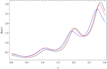
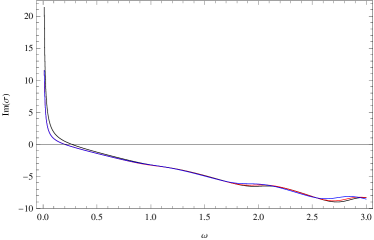
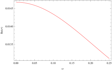
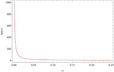
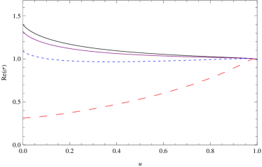
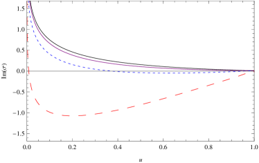
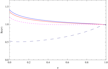
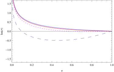
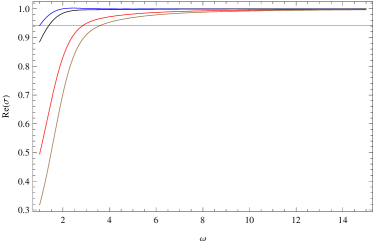
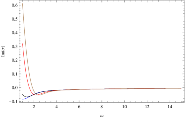
RG flow plots for AC conductivity has been shown in Fig.1. The frequency dependence of AC conductivity has been evaluated numerically and shown in Fig.3, Fig.4, Fig.5 and Fig.6. In the probe brane limit, taking , the plots in Fig. 3, show striking similarity with condensed matter systems Hartnoll:2008vx .
III Transport Coefficients with Gauss Bonnet Corrections
We study the effect of Gauss-Bonnet(GB) coupling on the RG flow of conductivity in the soft wall model approach. The modified action with the GB term is given by,
| (17) |
where is Gauss-Bonnet term and ‘’ is the Gauss Bonnet Coupling constant.
We consider the solution for Einstein-Maxwell-Gauss-Bonnet(EMGB) system as Cai:2001dz ; Cai:2009zv ; Buchel:2009sk ; Ge:2011fb ; Hu:2011ze .
| (18) |
where
and is related with the Gauss Bonnet coupling term as .
Using the membrane paradigm as explained above for the charged black hole case and perturbation of metric and gauge fields as in previous section, the modified equations of motion for vector perturbations are given by,
| (19) |
| (20) |
| (21) |
| (22) |
where .
In order to determine the flow equation of AC conductivity, we consider the current density with the GB corrections defined as,
| (23) |
The corresponding RG flow equation for AC conductivity (using definition (LABEL:cond))becomes,
| (24) |
In the near horizon limit, (the cut-off horizon), we can get an exact expression for the AC conductivity,
| (25) |
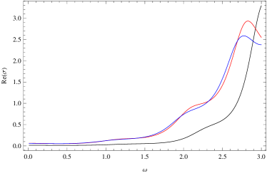
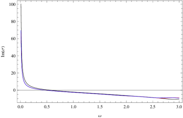
RG flow plots for AC conductivity with GB corrections has been shown in Fig.3 and we can notice that the qualitative feature of the flow are similar to the case without Gauss Bonnet correction.
IV Conclusions
The soft wall model of Holographic QCD is used here to get the insights into the transport properties like AC and DC conductivity in strongly coupled regime of QCD. The flow equations of AC and DC conductivity are considered for different values of chemical potential. The numerical solution of these equations enabled us to calculate the value of real and imaginary part of AC conductivity and the results seem to agree with the models, which consider the dynamics of condensate. This suggests that the soft wall model successfully captures the same features. This has also been noticed recently by Afonin:2015fga independently. In the probe limit our results (Fig.3) agree with existing results in the literature Hartnoll:2008vx ; Hartnoll:2009sz ; Matsuo:2011fk . The results at high frequency (Fig.4, Fig.5) show oscillatory behavior of AC conductivity, which is reminiscent of Shubnikov de Haas effect. At low frequency, the Drude behaviorDonos:2012js is observed (Fig.6). The Gauss-Bonnet coupling does not change the results significantly.
V Acknowledgement
We acknowledge the financial support from the DST, Govt. of India, Young Scientist project.
*
Appendix A DC CONDUCTIVITY
In order to calculate DC conductivity, we consider the gauge field equation (LABEL:cd) in the limit the equation of motion for gauge-field becomes,
| (26) |
The solution of , can be written as,
| (27) |
which can be used to calculate DC conductivity using the expression given in Iqbal:2008by ; Matsuo:2011fk
| (28) |
Thus, we get the following expression for DC conductivity flow,
In the near horizon region, , the DC conductivity takes the form,
| (29) |
At the boundary , DC flow is given as
| (30) |
Following the above procedure, we can consider the DC conductivity with Gauss-Bonnet corrections. We obtain the identical expression for DC conductivity indicating that the flow is independent of Gauss-Bonnet terms.
References
- (1) J. M. Maldacena, “The Large N limit of superconformal field theories and supergravity,” Ad v. Theor. Math. Phys. 2, 231 (1998) [hep-th/9711200], S. S. Gubser, I. R. Klebanov and A. M. Polyakov, “Gauge theory correlators from noncritical string theory,” Phys. Lett. B 428, 105 (1998) [hep-th/9802109],“Anti-de Sitter space and holography,” Adv. Theor. Math. Phys. 2, 253 (1998) [hep-th/9802150],
- (2) T. Sakai and S. Sugimoto, “Low energy hadron physics in holographic QCD,” Prog. Theor. Phys. 113, 843 (2005) [hep-th/0412141],
- (3) J. Erlich, E. Katz, D. T. Son and M. A. Stephanov, “QCD and a holographic model of hadrons,” Phys. Rev. Lett. 95, 261602 (2005) [hep-ph/0501128],L. Da Rold and A. Pomarol, “Chiral symmetry breaking from five dimensional spaces,” Nucl. Phys. B 721, 79 (2005) doi:10.1016/j.nuclphysb.2005.05.009 [hep-ph/0501218].
- (4) A. Karch, E. Katz, D. T. Son and M. A. Stephanov, “Linear confinement and AdS/QCD,” Phys. Rev. D 74, 015005 (2006) [hep-ph/0602229].
- (5) S. Sachan and S. Siwach, “Thermodynamics of soft wall AdS/QCD at finite chemical potential,” Mod. Phys. Lett. A 27, 1250163 (2012) doi:10.1142/S0217732312501635 [arXiv:1109.5523 [hep-th]].
- (6) D. T. Son and A. O. Starinets, “Minkowski space correlators in AdS / CFT correspondence: Recipe and applications,” JHEP 0209, 042 (2002) [hep-th/0205051]. G. Policastro, D. T. Son and A. O. Starinets, “From AdS / CFT correspondence to hydrodynamics,” JHEP 0209, 043 (2002) [hep-th/0205052].
- (7) P. Kovtun, D. T. Son and A. O. Starinets, “Holography and hydrodynamics: Diffusion on stretched horizons,” JHEP 0310, 064 (2003) [hep-th/0309213].
- (8) J. Erlich, “How Well Does AdS/QCD Describe QCD?,” Int. J. Mod. Phys. A 25, 411 (2010) [arXiv:0908.0312 [hep-ph]].
- (9) S. Jain, “Universal properties of thermal and electrical conductivity of gauge theory plasmas from holography,” JHEP 1006, 023 (2010) [arXiv:0912.2719 [hep-th]].
- (10) K. -i. Kim, Y. Kim, S. Takeuchi and T. Tsukioka, “Quark Number Susceptibility with Finite Quark Mass in Holographic QCD,” Prog. Theor. Phys. 126, 735 (2011) [arXiv:1012.2667 [hep-ph]].
- (11) M. Edalati, J. I. Jottar and R. G. Leigh, “Shear Modes, Criticality and Extremal Black Holes,” JHEP 1004, 075 (2010) [arXiv:1001.0779 [hep-th]].
- (12) D. Albrecht, C. D. Carone and J. Erlich, “Deconstructing Superconductivity,” Phys. Rev. D 86, 086005 (2012) doi:10.1103/PhysRevD.86.086005 [arXiv:1208.2700 [hep-th]].
- (13) A. Donos and S. A. Hartnoll, “Interaction-driven localization in holography,” Nature Phys. 9, 649 (2013) doi:10.1038/nphys2701 [arXiv:1212.2998].
- (14) N. Iqbal and H. Liu, “Universality of the hydrodynamic limit in AdS/CFT and the membrane paradigm,” Phys. Rev. D 79, 025023 (2009) [arXiv:0809.3808 [hep-th]].
- (15) I. Heemskerk and J. Polchinski, “Holographic and Wilsonian Renormalization Groups,” JHEP 1106, 031 (2011) [arXiv:1010.1264 [hep-th]].
- (16) Y. Matsuo, S. J. Sin, S. Takeuchi, T. Tsukioka and C. M. Yoo, “Sound Modes in Holographic Hydrodynamics for Charged AdS Black Hole,” Nucl. Phys. B 820, 593 (2009) [arXiv:0901.0610 [hep-th]].
- (17) I. Bredberg, C. Keeler, V. Lysov and A. Strominger, “Wilsonian Approach to Fluid/Gravity Duality,” JHEP 1103, 141 (2011) [arXiv:1006.1902 [hep-th]].
- (18) T. Faulkner, H. Liu and M. Rangamani, “Integrating out geometry: Holographic Wilsonian RG and the membrane paradigm,” JHEP 1108, 051 (2011) [arXiv:1010.4036 [hep-th]].
- (19) S. -J. Sin and Y. Zhou, “Holographic Wilsonian RG Flow and Sliding Membrane Paradigm,” JHEP 1105, 030 (2011) [arXiv:1102.4477 [hep-th]].
- (20) B. H. Lee, S. S. Pal and S. J. Sin, “RG flow of transport quantities,” Int. J. Mod. Phys. A 27, 1250071 (2012) [arXiv:1108.5577 [hep-th]].
- (21) Y. Matsuo, S. -J. Sin and Y. Zhou, “Mixed RG Flows and Hydrodynamics at Finite Holographic Screen,” JHEP 1201, 130 (2012) [arXiv:1109.2698 [hep-th]].
- (22) X. H. Ge, H. Q. Leng, L. Q. Fang and G. H. Yang, “Transport Coefficients for Holographic Hydrodynamics at Finite Energy Scale,” Adv. High Energy Phys. 2014, 915312 (2014) [arXiv:1408.4276 [hep-th]].
- (23) A. Chamblin, R. Emparan, C. V. Johnson and R. C. Myers, “Charged AdS black holes and catastrophic holography,” Phys. Rev. D 60, 064018 (1999) [hep-th/9902170].
- (24) X. H. Ge, Y. Matsuo, F. W. Shu, S. J. Sin and T. Tsukioka, “Density Dependence of Transport Coefficients from Holographic Hydrodynamics,” Prog. Theor. Phys. 120, 833 (2008) [arXiv:0806.4460 [hep-th]].
- (25) S. A. Hartnoll, C. P. Herzog and G. T. Horowitz, “Building a Holographic Superconductor,” Phys. Rev. Lett. 101, 031601 (2008) doi:10.1103/PhysRevLett.101.031601 [arXiv:0803.3295 [hep-th]].
- (26) R. G. Cai, “Gauss-Bonnet black holes in AdS spaces,” Phys. Rev. D 65, 084014 (2002) doi:10.1103/PhysRevD.65.084014 [hep-th/0109133].
- (27) R. G. Cai, Z. Y. Nie, N. Ohta and Y. W. Sun, “Shear Viscosity from Gauss-Bonnet Gravity with a Dilaton Coupling,” Phys. Rev. D 79, 066004 (2009) doi:10.1103/PhysRevD.79.066004 [arXiv:0901.1421 [hep-th]].
- (28) A. Buchel, J. Escobedo, R. C. Myers, M. F. Paulos, A. Sinha and M. Smolkin, “Holographic GB gravity in arbitrary dimensions,” JHEP 1003, 111 (2010) doi:10.1007/JHEP03(2010)111 [arXiv:0911.4257 [hep-th]].
- (29) X. -H. Ge, Y. Ling, Y. Tian and X. -N. Wu, “Holographic RG Flows and Transport Coefficients in Einstein-Gauss-Bonnet-Maxwell Theory,” JHEP 1201, 117 (2012) [arXiv:1112.0627 [hep-th]].
- (30) Y. P. Hu, P. Sun and J. H. Zhang, “Hydrodynamics with conserved current via AdS/CFT correspondence in the Maxwell-Gauss-Bonnet gravity,” Phys. Rev. D 83, 126003 (2011) doi:10.1103/PhysRevD.83.126003 [arXiv:1103.3773 [hep-th]].
- (31) S. S. Afonin and I. V. Pusenkov, “Soft wall model for a holographic superconductor,” arXiv:1506.05381 [hep-th].
- (32) S. A. Hartnoll, “Lectures on holographic methods for condensed matter physics,” Class. Quant. Grav. 26, 224002 (2009) doi:10.1088/0264-9381/26/22/224002 [arXiv:0903.3246 [hep-th]].