Long-distance synchronization of unidirectionally cascaded optomechanical systems

Abstract

Synchronization is of great scientific interest due to the abundant applications in a wide range of systems. We propose a scheme to achieve the controllable long-distance synchronization of two dissimilar optomechanical systems, which are unidirectionally coupled through a fiber with light. Synchronization, unsynchronization, and the dependence of the synchronization on driving laser strength and intrinsic frequency mismatch are studied based on the numerical simulation. Taking the fiber attenuation into account, it’s shown that two mechanical resonators can be synchronized over a distance of tens of kilometers. In addition, we also analyze the unidirectional synchronization of three optomechanical systems, demonstrating the scalability of our scheme.

I Introduction

Synchronization is a universal phenomenon in nature, where oscillators with different intrinsic frequencies can adjust their rhythms to oscillate in unison Pikovsky et al. (2001); Strogatz (2003). In 1660s, Huygens observed the synchronization of two pendulum clocks hanging on a same wall Nijhoff (1893). Since then, synchronization has been observed in a wide range of systems. For example, the coordination of neurons Izhikevich (2007) and the regular flash of glowworms colonies Buck and Buck (1968). Synchronization is of importance for both fundamental research and practical applications, since it has the capacity to improve the precision Cross (2012) of frequency sources built from (electro)mechanical oscillators in producing oscillating signals, which plays a critical role in time-keeping Sivrikaya and Yener (2004), sensing Bargatin et al. (2012) and communication Bregni (2002).

Synchronization has been demonstrated in many systems, such as Josephson junctions Cawthorne et al. (1999); Vlasov and Pikovsky (2013), micro- and nano- electromechanical systems Agrawal et al. (2013); Chen et al. (2013); Matheny et al. (2014); Antonio et al. (2015), ensembles of atoms Xu et al. (2014). Optomechanical system (OMS) Aspelmeyer et al. (2014a, b); Kippenberg and Vahala (2008) is one of such platforms for synchronization research Heinrich et al. (2011); Manipatruni et al. (2011); Ying et al. (2014); Li et al. (2015); Shah et al. (2015a), and holds great potential for applications due to the easily fabrication, high quality factor of optical resonators and strong optomechanical coupling. The synchronization of OMSs have been predicted theoretically Holmes et al. (2012) and demonstrated in experiments Zhang et al. (2012); Bagheri et al. (2013); Zhang et al. (2015). For example, in two silicon nitride microdisks, spaced apart by 400nm, two mechanical modes are synchronized by the coupling of two optical modes Zhang et al. (2012). Two spatially separated 80 micrometers nanomechanical oscillators are also synchronized through coupling to a same racetrack cavity Bagheri et al. (2013).

However, those OMSs are coupled through local optical coupling between cavities, while the greatest advantage of the light that can propagate over very long distance is overlooked. Very recently, a long-distance master-slave frequency locking has been realized between two OMSs Shah et al. (2015b), while the light output from one OMS is converted to radio frequency (RF) signal and the other OMS is injection locked by using an electro-optic modulator (EOM) to modulate the input laser. Extra elements required in this scheme, such as detectors and amplifiers will introduce noises to such system and may limit the stability of the system.

In this paper, we present a scheme to realize synchronization of cascaded OMSs, where two OMSs are coupled through light propagating unidirectionally in fiber, no extra detection of light is required. Through numerical simulation, we observe the synchronization phenomenon and study the influence of different systemic and external driving parameters on synchronization. In practical applications in long distance synchronization, we take the fiber attenuation into account, and confirm the synchronization is possible for two OMSs over tens of kilometers. Last but not least, we expand synchronization of two OMSs into synchronization of three OMSs, which verifies the feasibility of unidirectional synchronization of an OMSs array.

II Model

The unidirectionally cascaded synchronization scheme consists of two toroid optical microcavities Armani et al. (2003) with small mechanical frequency mismatch. Both toroids are cascaded coupled with the optical fiber, as shown in Fig. 1. The input laser in the fiber is coupled to the traveling optical whispering gallery modes in the former toroid, and the transmitted light is coupled to the following toroid. Each toroid also supports low loss mechanical breath vibration mode Schliesser et al. (2006), thus enables optomechanical coupling. In our model, it’s assumed that there is no laser input in the reversal direction, so the optical coupling between cascaded toroids are unidirectional. We would expect that light could carry the vibration information from the first optomechanical system (OMS-1) to the second optomechanical system (OMS-2), and thus enable the unidirectional synchronization.

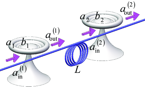
Figure 1: (Color online) Schematic setup of the unidirectionally cascaded systems of two toroid optical microcavities, coupled through a unidirectional fiber with light. The distance between the two OMSs is denoted as $L$.

The Hamiltonian of the individual OMS-$j$ ($j=1,2$) is

$$H_{j}=\hbar\omega_{cj}a_{j}^{\dagger}a_{j}+\hbar\omega_{mj}b_{j}^{\dagger}b_{j}-\hbar g_{j}a_{j}^{\dagger}a_{j}\left(b_{j}+b_{j}^{\dagger}\right),$$ (1)

where $a_{j}^{\dagger}$($b_{j}^{\dagger}$) and $a_{j}$($b_{j}$) are the optical (mechanical) creation and annihilation operators, frequencies of optical and mechanical mode are denoted as $\omega_{cj}$ and $\omega_{mj}$ respectively. The last term describes the dispersive coupling of optical mode and mechanical mode, where $g_{j}$ is the vacuum optomechanical coupling rate.

The dynamics of the unidirectionally cascaded OMSs are determined by the quantum Langevin equations, $\frac{\partial O}{\partial t}=\frac{1}{i\hbar}\left[O,H\right]+N-H_{diss}$, where $O$ is an arbitrary system operator, $N$ and $H_{diss}$ represent the environment noises and the system dissipation respectively. In the semiclassical cases, the mean values of the environment noises vanish, thus the equations of motion are as follows,

$$\dot{a}_{j} = \frac{1}{i\hbar}\left[a_{j},H_{j}\right]-\frac{\kappa_{j}}{2}a_{j}+\sqrt{\kappa_{exj}}a_{in}^{\left(j\right)},$$

$$\dot{b}_{j} = \frac{1}{i\hbar}\left[b_{j},H_{j}\right]-\frac{\gamma_{mj}}{2}b_{j},$$ (2)

where $j=1,2$. $\kappa_{j}$ and $\kappa_{exj}$ are the total and external optical decay rates, respectively. $\gamma_{mj}$ is the mechanical damping rate. $a_{in}^{\left(j\right)}$ represents the injected driving field.

Based on the properties of cascaded systems Gardiner (1993); Cirac et al. (1997); Tan et al. (2013),

$$a_{in}^{\left(2\right)}\left(t\right)=\eta_{12}a_{out}^{\left(1\right)}\left(t-\tau\right),$$ (3)

where $\eta_{12}=\sqrt{\eta_{P}}$ and $\eta_{P}$ is the power transmittance, $a_{out}^{\left(1\right)}\left(t-\tau\right)$ represents the output field of OMS-1, $\tau$ is the required time for light transmitting from OMS-1 to OMS-2. In the case of unidirectionally cascaded systems, only one direction for transmission is allowed. Thus, without loss of universality, we let $\tau\rightarrow 0_{+}$. Based on the input and output theory of optical cavities Walls and Milburn (2007),

$$a_{out}^{\left(1\right)}\left(t\right)=a_{in}^{\left(1\right)}\left(t\right)-\sqrt{\kappa_{ex1}}a_{1}.$$ (4)

Assuming $a_{in}^{\left(1\right)}\left(t\right)=E_{in}e^{-i\omega_{L}t}$, where $E_{in}$ and $\omega_{L}$ represent the strength and frequency of the driving optical field, respectively. In the rotating frame with the driving frequency $\omega_{L}$, define $\tilde{a}_{j}=a_{j}e^{i\omega_{L}t}$ ($j=1,2$), then based on Eq. (2), the optical and mechanical modes satisfy

$$\dot{\tilde{a}}_{1} = -(i\varDelta_{1}+\frac{\kappa_{1}}{2})\tilde{a}_{1}+ig_{1}\tilde{a}_{1}\left(b_{1}+b_{1}^{\dagger}\right)+E,$$ (5)

$$\dot{\tilde{a}}_{2} = -(i\varDelta_{2}+\frac{\kappa_{2}}{2})\tilde{a}_{2}+ig_{2}\tilde{a}_{2}\left(b_{2}+b_{2}^{\dagger}\right)$$ (6)

$$+\eta_{12}\sqrt{\kappa_{ex2}}\left(E/\sqrt{\kappa_{ex1}}-\sqrt{\kappa_{ex1}}\tilde{a}_{1}\right),$$

$$\dot{b}_{j} = -i\omega_{mj}b_{j}+ig_{j}\tilde{a}_{j}^{\dagger}\tilde{a}_{j}-\frac{\gamma_{mj}}{2}b_{j},\thinspace\thinspace j=1,2,$$ (7)

where $\varDelta_{j}=\omega_{cj}-\omega_{L}\thinspace(j=1,2)$ is the driving field detuning. $E=\sqrt{\kappa_{ex1}}E_{in}$ is the effective optical driving strength of OMS-1.

In addition, the equations of motion can also be derived consistently from the master equation Gardiner and Zoller (2004), indicating the time evolution of density matrix $\rho$,

$$\dot{\rho} = \frac{1}{i\hbar}\left[H_{1}+H_{2},\rho\right]+\kappa_{1}\mathcal{L}\left[a_{1}\right]\rho+\kappa_{2}\mathcal{L}\left[a_{2}\right]\rho$$ (8)

$$+\gamma_{m1}\mathcal{L}\left[b_{1}\right]\rho+\gamma_{m2}\mathcal{L}\left[a_{2}\right]\rho$$

$$+\sqrt{\kappa_{ex1}\kappa_{ex2}}\left\{\mathcal{L}\left[a_{1}+a_{2}\right]\rho+\frac{1}{2}\left[a_{1}^{\dagger}a_{2}-a_{2}^{\dagger}a_{1},\rho\right]\right\}$$

$$+\left[a_{in}^{\left(1\right)}\left(\sqrt{\kappa_{ex1}}a_{1}^{\dagger}+\sqrt{\kappa_{ex2}}a_{2}^{\dagger}\right)-h.c,\rho\right],$$

where $\mathcal{L}\left[o\right]\rho=o\rho o^{\dagger}-\frac{1}{2}\left(o^{\dagger}o\rho+\rho o^{\dagger}o\right)$ is the Lindblad superoperator. And the coupling term in the master equation consists of a damping term $\mathcal{L}\left[a_{1}+a_{2}\right]\rho$ and a commutator $\frac{1}{2}\left[a_{1}^{\dagger}a_{2}-a_{2}^{\dagger}a_{1},\rho\right]$, which indicates the system’s unidirectionality.

From equations of motion [Eqs. (5) and (6)], the output of OMS-1 drives the optical mode of OMS-2. In contrast, the output of OMS-2 has no effects on OMS-1. Due to the nonlinear interaction between optical mode and mechanical mode, such as $g_{1}\tilde{a}_{1}\left(b_{1}+b_{1}^{\dagger}\right)$ in Eq. (5), the output optical field from OMS-1 can modify the behavior of the mechanical resonator in OMS-2, and may lead to the synchronization. The dynamics of the system is significantly different from previously studied bidirectionally coupled OMSs, where the mutual coupling can induce the synchronization.

III Unidirectional synchronization

Since the nonlinear optomechanical interaction is crucial in the synchronization, we don’t apply linear approximations to solve the equations of motion. The full dynamics of unidirectionally cascaded systems are simulated for long evolution time numerically. For the convenient to illustrate the synchronization, the optical and mechanical operators are re-written as

$$\begin{array}[]{cccccc}Q_{j}&=&\left(\tilde{a}_{j}+\tilde{a}_{j}^{\dagger}\right)/2,&P_{j}&=&-i\left(\tilde{a}_{j}-\tilde{a}_{j}^{\dagger}\right)/2,\\ q_{j}&=&\left(b_{j}+b_{j}^{\dagger}\right)/\sqrt{2},&p_{j}&=&-i\left(b_{j}-b_{j}^{\dagger}\right)/\sqrt{2},\end{array}$$ (9)

where $j=1,2$. And the corresponding equations for quadratures of optical fields $Q_{j},\thinspace P_{j}$ and mechanical displacement $q_{j}$ and momentum $p_{j}$ read

$$\dot{Q}_{1} = \left(\varDelta_{1}-G_{1}q_{1}\right)P_{1}-\frac{\kappa_{1}}{2}Q_{1}+E,$$

$$\dot{P}_{1} = -\left(\varDelta_{1}-G_{1}q_{1}\right)Q_{1}-\frac{\kappa_{1}}{2}P_{1},$$

$$\dot{Q}_{2} = \left(\varDelta_{2}-G_{2}q_{2}\right)P_{2}-\frac{\kappa_{2}}{2}Q_{2}+$$

$$\sqrt{\kappa_{ex2}}\left(E/\sqrt{\kappa_{ex1}}-\sqrt{\kappa_{ex1}}Q_{1}\right),$$

$$\dot{P}_{2} = -\left(\varDelta_{2}-G_{2}q_{2}\right)Q_{2}-\frac{\kappa_{2}}{2}P_{2}-\sqrt{\kappa_{ex2}\kappa_{ex1}}P_{1},$$

$$\dot{q}_{j} = \omega_{mj}p_{j},$$

$$\dot{p}_{j} = -\omega_{mj}q_{j}-\gamma_{mj}p_{j}+G_{j}\left(\tilde{a}_{jr}^{2}+\tilde{a}_{ji}^{2}\right),$$ (10)

where $G_{j}=\sqrt{2}g_{j}$. The numerical simulation is performed using the four-order Runge-Kutta algorithm. In the simulation, we choose realistic values of the parameters Li et al. (2015); Aspelmeyer et al. (2014a) and normalize them by $\omega_{m1}$: $\omega_{m1}=1,$ $\omega_{m2}=1.005,$ i.e., the intrinsic frequency of OMS-2 differs from that of OMS-1 with a mismatch of $5\permil\omega_{m1}$. $\varDelta_{1}=-\omega_{m1}$, $\varDelta_{2}=-\omega_{m2}$, i.e., the driving laser is blue detuned, which guarantees that OMS-1 will evolve into self-sustained oscillation as long as the driving strength is strong enough. The other parameters are $G_{1}=G_{2}=4\times 10^{-3}$, $\kappa_{1}=\kappa_{2}=0.15,$ $\kappa_{ex1}=\frac{\kappa_{1}}{2}$, $\kappa_{ex2}=\frac{\kappa_{2}}{2}$, $\gamma_{m1}=\gamma_{m2}=5\times 10^{-3}$. In addition, the time scale in the simulation becomes dimensionless and changes from $t$ into $t^{\prime}=\omega_{m1}t$ due to the normalization.

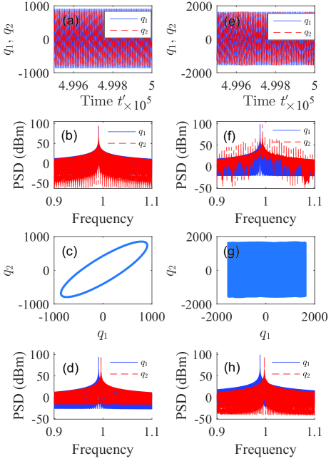
Figure 2: (Color online) Numerical solutions of equations of motion in the unidirectionally cascaded two OMSs scheme, for the parameters: $\omega_{m1}=1$, $\omega_{m2}=1.005$, $\varDelta_{1}=-\omega_{m1}$, $\varDelta_{2}=-\omega_{m2}$, $G_{1}=G_{2}=4\times 10^{-3},$ $\kappa_{1}=\kappa_{2}=0.15,$ $\kappa_{ex1}=\kappa_{ex2}=0.075$, $\gamma_{m1}=\gamma_{m2}=5\times 10^{-3}$. (a) and (e) Dynamical evolution. (b) and (f) Power spectrum density (PSD) of the displacement operators $q_{1}$ and $q_{2}$. (c) and (g) Phase diagram of $q_{1}$, $q_{2}$. (d) and (h) Displacement PSD of each single OMS driven by a constant amplitude optical field $E$. The left and right columns correspond to $E=64$ and $E=100$.

Firstly, we study the general properties of lossless cascade coupling between two OMSs. Figure 2 shows typical behaviors of the OMSs for different parameters. Under the effective driving of $E=64$, the dynamical evolution of mechanical displacement for two OMSs are shown in Fig. 2(a), and the corresponding power spectrum density (PSD) and phase diagram are shown in Fig. 2(b) and Fig. 2(c), respectively. Although the intrinsic mechanical frequencies are different by $5\permil$, the eventual oscillation frequencies are the same $\omega^{\prime}_{m1}=\omega^{\prime}_{m2}=0.990932$. The regular orbit in phase diagram confirms that the oscillation periods are exactly the same and their phase difference is constant. To exclude the possible coincidence that the self-oscillation frequencies of two OMSs under external optical driving are the same, we also plot the PSD for OMSs individually driven by the external laser in Fig. 2(d). The steady state oscillation frequencies are $\omega^{\prime}_{m1}=0.990932$, $\omega^{\prime}_{m2}=0.995881$, which are different by about $5\permil$ similar to that of intrinsic frequencies. The results confirm that $\omega^{\prime}_{m1}$ are exactly the same as $\omega_{m1}$ and not affected by the OMS-2, and the OMS-2 is synchronized to OMS-1 under the unidirectional optical coupling.

With a further increase in the strength of the laser driving the OMSs, the two OMSs are not guaranteed to be synchronized under the unidirectional coupling. As shown in Figs. 2(e)-2(h), the OMSs are unsynchronized for $E=100$. From the PSD, the OMS-1 is still unaffected by the OMS-2, just shows a single peak self-oscillation behavior. However, the PSD of OMS-2 [Fig. 2(f)] shows multiple peaks when driven by the output from OMS-1. The frequency locations of those peaks show equal distances. This can be interpreted as the dynamics of OMS-2 can still be greatly affected by OMS-1 for large laser driving, but nonlinear effect generates the frequency mixing of two systems instead of synchronization, which is a typical feature of the well-known nonlinear periodic pulling Koepke and Hartley (1991); Klinger et al. (1995); Menzel et al. (2011).

It is quite straightforward that there is also a threshold for nonlinear optomechanical interaction to make synchronization happen. The above results also indicate that the synchronization effect can only dominate the other nonlinear effects in certain driving laser amplitudes. For example, very strong nonlinear effect will induce multi-stable and even chaotic dynamics. Therefore, we further study the final frequencies $\omega^{\prime}_{m1}$, $\omega^{\prime}_{m2}$ as functions of the effective driving strength $E$. For each $E$, we try 10 sets of different random initial values of the system to test the sensitivity of the synchronization to initial conditions.

In Fig. 3, the PSD of $q_{1}$ and the PSD of $q_{2}$ but shifted in respect to the spectrum of $q_{1}$ are plotted. The results reveals different dynamical regimes for unidirectionally coupled OMSs: (1) Weak nonlinear effect, $E\in\left[10,37\right]$. Below the threshold of about $E\approx 37$, the two OMSs are unsynchronized $\omega^{\prime}_{m2}\neq\omega^{\prime}_{m1}$. However, the OMS-2 are affected by the mechanical oscillation in OMS-1, thus a series of sidebands appear in the PSD of $q_{2}$. (2) Synchronization, $E\in\left[38,96\right]$. For moderate driving, the two OMSs are synchronized with a sole peak in the PSD of $q_{2}$ and $\omega^{\prime}_{m2}=\omega^{\prime}_{m1}$. (3) Multi-stable and chaotic regime, $E\in\left[97,160\right]$. For very strong driving, the two OMSs are unsynchronized. There are multiple possible self-oscillation frequencies of OMS-1. For certain OMS-1 oscillation frequency, the OMS-2 can still be synchronized. While, for other frequencies, the OMS-2 exhibits very complex dynamics, including synchronization, frequency mixing and multi-stable dynamics simultaneously.

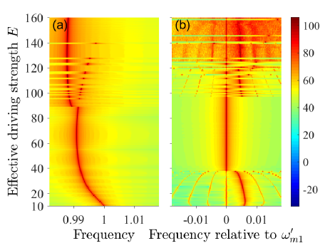
Figure 3: (Color online) (a) The PSD of $q_{1}$ as a function of the effective driving strength $E$, with a sole frequency peak denoted as $\omega^{\prime}_{m1}$. (b) The PSD of $q_{2}$ relative to $\omega^{\prime}_{m1}$ as a function of the effective driving strength $E$. The maximum frequency component in the PSD of $q_{2}$ without the frequency shift is denoted as $\omega^{\prime}_{m2}$. The color scaled in the color bar indicates the power values in the PSD. The other simulation parameters are the same as those in Fig. 2.

Actually, due to the unidirectionality, OMS-1 is independent from OMS-2 and thus can be fully theoretically solved using the single OMS theory Marquardt et al. (2006) and the output field is modulated by the mechanical vibration. The observed synchronization and periodic pulling phenomena of OMS-2 originate from the modulated laser driving on OMS-2. Similar effects have been demonstrated with the injection-locking Adler (1946); Razavi (2004); Knünz et al. (2010) of an OMS Shlomi et al. (2015); Hossein-Zadeh and Vahala (2008); Shah et al. (2015b), where the input laser of the OMS is partially modulated by a single tone RF signal using an electro-optic modulator.

Previous studies show that synchronization occurs only when the driving RF frequency is very close to the intrinsic oscillation frequency Klinger et al. (1995). Inspirited by this, the final relative frequency difference $\left(\omega^{\prime}_{m2}-\omega^{\prime}_{m1}\right)/\omega^{\prime}_{m1}$ as a function of the intrinsic frequency mismatch $\left(\omega_{m2}-\omega_{m1}\right)/\omega_{m1}$ is plotted in Fig. 4. When $E=64$ ($E=40$), there is a synchronization region of $\omega_{m2}\in\left[1-9.2\permil,1+8.2\permil\right]\omega_{m1}$ ($\omega_{m2}\in\left[1-8\permil,1+5.6\permil\right]\omega_{m1}$), represented by the red line (the blue line). We find that, the width of synchronization region is similar to the mechanical damping rate $5\permil$ Hossein-Zadeh and Vahala (2008), and the increase of driving strength does enlarge the width of synchronization region, by comparing the results of $E=64$ and that of $E=40$.

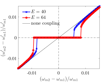
Figure 4: (Color online) The final relative frequency difference between the maximum frequency components of two OMSs $\left(\omega^{\prime}_{m2}-\omega^{\prime}_{m1}\right)/\omega^{\prime}_{m1}$ vs the relative intrinsic frequency mismatch $\left(\omega_{m2}-\omega_{m1}\right)/\omega_{m1}$. Blue solid line marked with ’x’: $E=40$. Red solid line marked with ’o’: $E=64$. Black solid line: uncoupled free-running case.

IV Long distance unidirectional synchronization with fiber-loss

The unidirectional coupling is very potential for future long distance synchronization, since the OMSs are directly coupled through the optical connections, without extra optical-to-electronic or reversal conversion processes. In addition, the unidirectional coupling also greatly reduces the complexity of experiments. To testify the potential for long distance synchronization, we take the practical fiber attenuation loss into our model. Take 1550nm light as an example, the propagation loss rate is $\alpha=0.2\thinspace{\rm dB}/{\rm km}$, the power transmittance $\eta_{P}=10^{-\alpha L/10}$.

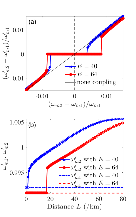
Figure 5: (Color online) Considering fiber-loss, (a) the final relative frequency difference between the maximum frequency components of the two OMSs $\left(\omega^{\prime}_{m2}-\omega^{\prime}_{m1}\right)/\omega^{\prime}_{m1}$ vs the relative intrinsic frequency mismatch $\left(\omega_{m2}-\omega_{m1}\right)/\omega_{m1}$ with $L=4.6\thinspace{\rm km}$, $\eta_{12}=0.9$. The cases corresponding to the lines are the same as those in Fig. 4. (b) The final maximum frequency components of the two OMSs $\omega^{\prime}_{m1}$, $\omega^{\prime}_{m2}$ vs distance $L$. Blue solid line marked with ’x’: $\omega^{\prime}_{m2}$ with $E=40$. Red solid line marked with ’o’: $\omega^{\prime}_{m2}$ with $E=64$. Blue dash-dotted line: $\omega^{\prime}_{m1}$ with $E=40$. Red dashed line: $\omega^{\prime}_{m1}$ with $E=64$.

First, take $L=4.6\,\mathrm{km}$, i.e., $\eta_{12}=\sqrt{\eta_{P}}=0.9$, synchronization region of $\omega_{m2}\in\left[1-8.4\permil,1+8.2\permil\right]\omega_{m1}$ ($\omega_{m2}\in\left[1-7.4\permil,1+3.8\permil\right]\omega_{m1}$) is revealed for $E=64$ ($E=40$) [Fig. 5(a)]. Compared to the result without fiber loss $\eta_{P}=1.0$ in Fig. 4, the parameter region has shrunk. Then, we explore whether the systems are synchronized or not for $L$ varying from 0 to 80km, while fixing the intrinsic mechanical frequencies $\omega_{m1}=1,$ $\omega_{m2}=1.005$. As plotted in Fig. 5(b), we can see for each $E$ there exists a critical distance $L_{cri}$, over which the state of two OMSs changes from synchronization into unsynchronization. The critical distance for $E=40$ and $E=64$ are as long as 1.3 km and 16.7 km, respectively, which verifies the capability of our scheme to realize long-distance unidirectional synchronization.

V Unidirectional synchronization of three OMSs

Now, we further study the generalized unidirectional synchronization of a cascaded OMSs array. From the results of two OMSs, the synchronization is possible for additional OMSs following OMS-2, as long as the driving laser intensity on them is moderate and contains the components of modulation from the mechanical vibrations. As an example, the unidirectional synchronization scheme of three dissimilar OMSs (microtoroids) with different intrinsic frequencies are cascaded using a unidirectional fiber, as shown in Fig. 6.

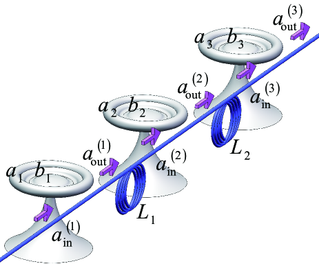
Figure 6: (Color online) Schematic setup of the unidirectionally cascaded synchronization scheme consists of three OMSs. The distance between the first (last) two OMSs is denoted as $L_{1}$ ($L_{2}$).

Let $\eta_{23}=a_{in}^{\left(3\right)}/a_{out}^{\left(2\right)}$, $\eta_{12}=a_{in}^{\left(2\right)}/a_{out}^{\left(1\right)}$, the set of equations of motion can be obtained, where $\dot{\tilde{a}}_{1}$, $\dot{\tilde{a}}_{2}$, $\dot{b}_{1}$ and $\dot{b}_{2}$ are the same as Eqs.(5,6,7) due to the unidirectionality, and $\dot{\tilde{a}}_{3}$ and $\dot{b}_{3}$ are in the following form,

$$\dot{\tilde{a}}_{3} = -i\left(\varDelta_{3}+\frac{\kappa_{3}}{2}\right)\tilde{a}_{3}+ig_{3}\tilde{a}_{3}\left(b_{3}+b_{3}^{\dagger}\right)$$

$$+\eta_{23}\eta_{12}\sqrt{\kappa_{ex3}}\left(E/\sqrt{\kappa_{ex1}}-\sqrt{\kappa_{ex1}}\tilde{a}_{1}\right)$$

$$-\eta_{23}\sqrt{\kappa_{ex3}\kappa_{ex2}}\tilde{a}_{2},$$

$$\dot{b}_{3} = -i\omega_{m3}b_{3}+ig_{3}\tilde{a}_{3}^{\dagger}\tilde{a}_{3}-\frac{\gamma_{m3}}{2}b_{3}.$$ (11)

Following the similar procedure of numerical simulation for two OMSs, the dynamics of the three OMSs are solved. Shown in Fig. 7(a) (Fig. 7(b)) the PSDs of $q_{1}$, $q_{2}$ and $q_{3}$ under a set of parameters: $\omega_{m2}=0.995$, $\omega_{m3}=1.005$ ($\omega_{m2}=1.005$, $\omega_{m3}=1.010$) are plotted. The other simulation parameters are $E=64$, $\omega_{m1}=1$, $\eta_{12}=\eta_{23}=1$, $\varDelta_{1}=\varDelta_{2}=\varDelta_{3}=-\omega_{m1}$, $G_{1}=G_{2}=G_{3}=0.004,$ $\kappa_{1}=\kappa_{2}=\kappa_{3}=0.15,$ $\kappa_{ex1}=\kappa_{ex2}=\kappa_{ex3}=0.075$, $\gamma_{m1}=\gamma_{m2}=\gamma_{m3}=0.005$. In Fig. 7(a), the three OMSs are all synchronized, while in Fig. 7(b) OMS-2 other than OMS-3 is synchronized to OMS-1. i.e., the three OMSs are partially synchronized.

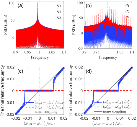
Figure 7: (Color online) Numerical solutions of the equations of motion in the unidirectionally cascaded three OMSs scheme. (a) and (b) The PSDs of $q_{1}$, $q_{2}$ and $q_{3}$. The parameters are: (a) $\omega_{m2}=0.995$, $\omega_{m3}=1.005$, (b) $\omega_{m2}=1.005$, $\omega_{m3}=1.010$. (c) and (d) The synchronization region of $\omega_{m3}$ relative to $\omega_{m1}$. The parameters are: (c) $\omega_{m1}=1$, $\omega_{m2}=0.995$, (d) $\omega_{m1}=1$, $\omega_{m2}=1.005$.

In addition, for a fixed effective driving strength $E=64$ and $\omega_{m1}=1$, when $\omega_{m2}=0.995$ ($\omega_{m2}=1.005$), the synchronization region of $\omega_{m3}\in\left[1-12.4\permil,1+11.2\permil\right]\omega_{m1}$ ($\omega_{m3}\in\left[1-12\permil,1+8.6\permil\right]\omega_{m1}$) can be obtained by traversing $\omega_{m3}\in\left[0.98,1.02\right]$, as shown in Fig. 7(c) (Fig. 7(d)). Comparing the synchronization region of the three OMSs scheme with that of the two OMSs scheme [Fig. 4], we find that the synchronization region has expanded to some extent at certain values of $\omega_{m2}$. Thus, the synchronization of three OMSs is available, which verifies the feasibility of synchronization of an array of more than 2 cascaded OMSs.

VI Conclusion

We have demonstrated the synchronization of optomechanical systems by all-optical method, where the systems are coupled through light propagating unidirectionally in the fiber. For two OMSs with fixed mechanical frequency mismatch, synchronization can be tuned on or off through tuning the optical driving strength. For a fixed driving strength, there exists a region of mechanical frequency mismatch that allows for the synchronization. And in the practical cases, the synchronization can still be achieved for distance over 10 km, while the synchronization region shrinks due to the light attenuates when travel over long distances. Unidirectional synchronization of three OMSs is also obtained, as well. The all-optical feature, high controllability, wide synchronization region, long synchronization distance, and novel scalability of our scheme are appealing and can be useful for many applications, such as the construction of complex synchronization OMSs networks Zhang et al. (2015). We expected that the scheme also works for other optomechanical interactions, such as quadratic Lee et al. (2015) , dissipative Li et al. (2009); Zou et al. (2011) and Brillouin Dong et al. (2015); Kim et al. (2015) optomechanical interactions.

References

- Pikovsky et al. (2001) A. Pikovsky, M. Rosenblum, and J. Kurths, Synchronization: a universal concept in nonlinear sciences, Vol. 12 (Cambridge university press, 2001).
- Strogatz (2003) S. Strogatz, Sync: The emerging science of spontaneous order (Hyperion, 2003).
- Nijhoff (1893) M. Nijhoff, Societe Hollandaise des Sciences, The Hague, The Netherlands 5, 243 (1893).
- Izhikevich (2007) E. M. Izhikevich, Dynamical systems in neuroscience (MIT press, 2007).
- Buck and Buck (1968) J. Buck and E. Buck, Science 159, 1319 (1968).
- Cross (2012) M. C. Cross, Phys. Rev. E 85, 046214 (2012).
- Sivrikaya and Yener (2004) F. Sivrikaya and B. Yener, IEEE Netw. 18, 45 (2004).
- Bargatin et al. (2012) I. Bargatin, E. Myers, J. Aldridge, C. Marcoux, P. Brianceau, L. Duraffourg, E. Colinet, S. Hentz, P. Andreucci, and M. Roukes, Nano Lett. 12, 1269 (2012).
- Bregni (2002) S. Bregni, Synchronization of digital telecommunications networks (Wiley New York, 2002).
- Cawthorne et al. (1999) A. B. Cawthorne, P. Barbara, S. V. Shitov, C. J. Lobb, K. Wiesenfeld, and A. Zangwill, Phys. Rev. B 60, 7575 (1999).
- Vlasov and Pikovsky (2013) V. Vlasov and A. Pikovsky, Phys. Rev. E 88, 022908 (2013).
- Agrawal et al. (2013) D. K. Agrawal, J. Woodhouse, and A. A. Seshia, Phys. Rev. Lett. 111, 084101 (2013).
- Chen et al. (2013) Q. Chen, Y.-C. Lai, J. Chae, and Y. Do, Phys. Rev. B 87, 144304 (2013).
- Matheny et al. (2014) M. H. Matheny, M. Grau, L. G. Villanueva, R. B. Karabalin, M. C. Cross, and M. L. Roukes, Phys. Rev. Lett. 112, 014101 (2014).
- Antonio et al. (2015) D. Antonio, D. A. Czaplewski, J. R. Guest, D. López, S. I. Arroyo, and D. H. Zanette, Phys. Rev. Lett. 114, 034103 (2015).
- Xu et al. (2014) M. Xu, D. A. Tieri, E. C. Fine, J. K. Thompson, and M. J. Holland, Phys. Rev. Lett. 113, 154101 (2014).
- Aspelmeyer et al. (2014a) M. Aspelmeyer, T. J. Kippenberg, and F. Marquardt, Rev. Mod. Phys. 86, 1391 (2014a).
- Aspelmeyer et al. (2014b) M. Aspelmeyer, T. J. Kippenberg, and F. Marquardt, Cavity Optomechanics: Nano-and Micromechanical Resonators Interacting with Light (Springer, 2014).
- Kippenberg and Vahala (2008) T. J. Kippenberg and K. J. Vahala, Science 321, 1172 (2008).
- Heinrich et al. (2011) G. Heinrich, M. Ludwig, J. Qian, B. Kubala, and F. Marquardt, Phys. Rev. Lett. 107, 043603 (2011).
- Manipatruni et al. (2011) S. Manipatruni, G. Weiderhecker, and M. Lipson, in Quantum Electronics and Laser Science Conf. (Opt. Soc. Am, 2011) p. QWI1.
- Ying et al. (2014) L. Ying, Y.-C. Lai, and C. Grebogi, Phys. Rev. A 90, 053810 (2014).
- Li et al. (2015) W. Li, C. Li, and H. Song, J. Phys. B 48, 035503 (2015).
- Shah et al. (2015a) S. Y. Shah, M. Zhang, R. Rand, and M. Lipson, arXiv:1511.08536 (2015a).
- Holmes et al. (2012) C. A. Holmes, C. P. Meaney, and G. J. Milburn, Phys. Rev. E 85, 066203 (2012).
- Zhang et al. (2012) M. Zhang, G. S. Wiederhecker, S. Manipatruni, A. Barnard, P. McEuen, and M. Lipson, Phys. Rev. Lett. 109, 233906 (2012).
- Bagheri et al. (2013) M. Bagheri, M. Poot, L. Fan, F. Marquardt, and H. X. Tang, Phys. Rev. Lett. 111, 213902 (2013).
- Zhang et al. (2015) M. Zhang, S. Shah, J. Cardenas, and M. Lipson, Phys. Rev. Lett. 115, 163902 (2015).
- Shah et al. (2015b) S. Y. Shah, M. Zhang, R. Rand, and M. Lipson, Phys. Rev. Lett. 114, 113602 (2015b).
- Armani et al. (2003) D. Armani, T. Kippenberg, S. Spillane, and K. Vahala, Nature (London) 421, 925 (2003).
- Schliesser et al. (2006) A. Schliesser, P. Del’Haye, N. Nooshi, K. J. Vahala, and T. J. Kippenberg, Phys. Rev. Lett. 97, 243905 (2006).
- Gardiner (1993) C. W. Gardiner, Phys. Rev. Lett. 70, 2269 (1993).
- Cirac et al. (1997) J. I. Cirac, P. Zoller, H. J. Kimble, and H. Mabuchi, Phys. Rev. Lett. 78, 3221 (1997).
- Tan et al. (2013) H. Tan, L. F. Buchmann, H. Seok, and G. Li, Phys. Rev. A 87, 022318 (2013).
- Walls and Milburn (2007) D. F. Walls and G. J. Milburn, Quantum optics (Springer Science & Business Media, 2007).
- Gardiner and Zoller (2004) C. Gardiner and P. Zoller, Quantum noise: a handbook of Markovian and non-Markovian quantum stochastic methods with applications to quantum optics, Vol. 56 (Springer Science & Business Media, 2004).
- Koepke and Hartley (1991) M. E. Koepke and D. M. Hartley, Phys. Rev. A 44, 6877 (1991).
- Klinger et al. (1995) T. Klinger, F. Greiner, A. Rohde, A. Piel, and M. E. Koepke, Phys. Rev. E 52, 4316 (1995).
- Menzel et al. (2011) K. O. Menzel, O. Arp, and A. Piel, Phys. Rev. E 84, 016405 (2011).
- Marquardt et al. (2006) F. Marquardt, J. G. E. Harris, and S. M. Girvin, Phys. Rev. Lett. 96, 103901 (2006).
- Adler (1946) R. Adler, Proc. IEEE 34, 351 (1946).
- Razavi (2004) B. Razavi, IEEE J. Solid-State Circuit 39, 1415 (2004).
- Knünz et al. (2010) S. Knünz, M. Herrmann, V. Batteiger, G. Saathoff, T. W. Hänsch, K. Vahala, and T. Udem, Phys. Rev. Lett. 105, 013004 (2010).
- Shlomi et al. (2015) K. Shlomi, D. Yuvaraj, I. Baskin, O. Suchoi, R. Winik, and E. Buks, Phys. Rev. E 91, 032910 (2015).
- Hossein-Zadeh and Vahala (2008) M. Hossein-Zadeh and K. J. Vahala, Appl. Phys. Lett. 93, 191115 (2008).
- Lee et al. (2015) D. Lee, M. Underwood, D. Mason, A. Shkarin, S. Hoch, and J. Harris, Nat. Commun. 6, 6232 (2015).
- Li et al. (2009) M. Li, W. H. P. Pernice, and H. X. Tang, Phys. Rev. Lett. 103, 223901 (2009).
- Zou et al. (2011) C.-L. Zou, X.-B. Zou, F.-W. Sun, Z.-F. Han, and G.-C. Guo, Phys. Rev. A 84, 032317 (2011).
- Dong et al. (2015) C.-H. Dong, Z. Shen, C.-L. Zou, Y.-L. Zhang, W. Fu, and G.-C. Guo, Nat. Commun. 6, 6193 (2015).
- Kim et al. (2015) J. Kim, M. C. Kuzyk, K. Han, H. Wang, and G. Bahl, Nat. Phys. 11, 275 (2015).