A new discretization for $m$th-Laplace equations
with arbitrary polynomial degrees

Abstract

This paper introduces new mixed formulations and discretizations for $m$th-Laplace equations of the form $(-1)^{m}\Delta^{m}u=f$ for arbitrary $m=1,2,3,\dots$ based on novel Helmholtz-type decompositions for tensor-valued functions. The new discretizations allow for ansatz spaces of arbitrary polynomial degree and the lowest-order choice coincides with the non-conforming FEMs of Crouzeix and Raviart for $m=1$ and of Morley for $m=2$. Since the derivatives are directly approximated, the lowest-order discretizations consist of piecewise affine and piecewise constant functions for any $m=1,2,\dots$ Moreover, a uniform implementation for arbitrary $m$ is possible. Besides the a priori and a posteriori analysis, this paper proves optimal convergence rates for adaptive algorithms for the new discretizations.

Keywords $m$th-Laplace equation, polyharmonic equation, non-conforming FEM, mixed FEM, adaptive FEM, optimality

AMS subject classification 31A30, 35J30, 65N30, 65N12, 74K20

1 Introduction

This paper considers $m$th-Laplace equations of the form

$$(-1)^{m}\Delta^{m}u=f$$ (1.1)

for arbitrary $m=1,2,3,\dots$ Standard conforming FEMs require ansatz spaces in $H^{m}_{0}(\Omega)$. To circumvent those high regularity requirements and resulting complicated finite elements, non-standard methods are of high interest [Mor68, EGH⁺02, Bre12, GN11]. The novel Helmholtz decomposition of this paper decomposes any (tensor-valued) $L^{2}$ function in an $m$th derivative and a symmetric part of a Curl. Given a tensor-valued function $\varphi$ which satisfies $-\operatorname{div}^{m}\varphi=f$ in the weak sense, the $L^{2}$ projection of $\varphi$ to the space $D^{m}H^{m}_{0}(\Omega)$ of $m$th derivatives then coincides with the $m$th derivative of the exact solution of (1.1) (see Theorem 5.1 below). This results in novel mixed formulations and discretizations for (1.1). This approach generalises the discretizations of [Sch15, Sch16] from $m=1$ to $m\geq 1$.

The direct approximation of $D^{m}u$ instead of $u$ enables low order discretizations; only first derivatives appear in the symmetric part of the Curl and so the lowest order approach only requires piecewise affine functions for any $m$. In contrast to that, even interior penalty methods require piecewise quadratic [Bre12] resp. piecewise cubic [GN11] functions for $m=2$ resp. $m=3$. Mnemonic diagrams in Figure 1 illustrate lowest-order standard conforming FEMs from [Žen70] and the lowest-order novel FEMs proposed in this work for $m=2,3$. Since the proposed new FEMs differ only in the number of components in the ansatz spaces, an implementation of one single program, which runs for arbitrary order, is possible. In particular, the system matrices are obtained by integration of standard FEM basis functions.

Figure 1: Lowest order standard conforming [Cia78, Žen70] and novel FEMs for the problem $(-1)^{m}\Delta^{m}u=f$ for $m=2,3$.

For $m=1,2$ and the lowest polynomial degree in the ansatz spaces, discrete Helmholtz decompositions of [AF89, CGH14] prove that the discrete solutions are piecewise gradients (resp. Hessians) of Crouzeix-Raviart [CR73] (resp. Morley [Mor68]) finite element functions and therefore the new discretizations can be regarded as a generalization of those non-conforming FEMs to higher polynomial degrees and higher-order problems. The generalization of [WX13] of the non-conforming Crouzeix-Raviart and Morley FEMs to $m\geq 3$ is restricted to a space dimension $\geq m$.

In the context of the novel (mixed) formulations, the discretizations appear to be conforming. The new generalization to higher polynomial degrees proposed in this paper appears to be natural in the sense that the inherent properties of the lowest order discretization carry over to higher polynomial ansatz spaces, namely an inf-sup condition, the conformity of the method, and a crucial projection property (also known as integral mean property of the non-conforming interpolation operator).

Besides the a priori and a posteriori error analysis, this paper proves optimal convergence rates for an adaptive algorithm, which are also observed in the numerical experiments from Section 7.

The remaining parts of this paper are organised as follows. Section 2 introduces some notation while some preliminary results are proved in Section 3. The proposed discretization of (1.1) in Section 5 is based on a novel Helmholtz decomposition for higher derivatives which is stated and proved in Section 4. Section 6 introduces an adaptive algorithm and proves optimal convergence rates. Section 7 concludes the paper with numerical experiments on fourth- and sixth-order problems.

Throughout this paper, let $\Omega\subseteq\mathbb{R}^{2}$ be a bounded, polygonal, simply connected Lipschitz domain. Standard notation on Lebesgue and Sobolev spaces and their norms is employed with $L^{2}$ scalar product $(\bullet,\bullet)_{L^{2}(\Omega)}$. Given a Hilbert space $X$, let $L^{2}(\Omega;X)$ resp. $H^{k}(\Omega;X)$ denote the space of functions with values in $X$ whose components are in $L^{2}(\Omega)$ resp. $H^{k}(\Omega)$. The space of infinitely differentiable functions reads $C^{\infty}(\Omega)$ and the subspace of functions with compact support in $\Omega$ is denoted with $C^{\infty}_{c}(\Omega)$. The piecewise action of differential operators is denoted with a subscript $\mathrm{NC}$. The formula $A\lesssim B$ represents an inequality $A\leq CB$ for some mesh-size independent, positive generic constant $C$; $A\approx B$ abbreviates $A\lesssim B\lesssim A$. By convention, all generic constants $C\approx 1$ do neither depend on the mesh-size nor on the level of a triangulation but may depend on the fixed coarse triangulation $\mathcal{T}_{0}$ and its interior angles.

2 Notation

This section introduces notation related to higher-order tensors and tensor-valued functions and triangulations.

Define the set of $\ell$-tensors over $\mathbb{R}^{2}$ by

$$\mathbb{X}(\ell):=\begin{cases}\mathbb{R}&\text{ for }\ell=0,\\ \prod_{j=1}^{\ell}\mathbb{R}^{2}=\mathbb{R}^{2}\times\dots\times\mathbb{R}^{2}\cong\mathbb{R}^{2^{\ell}}&\text{ for }\ell\geq 1\end{cases}$$

and let $\mathfrak{S}_{\ell}:=\{\sigma:\{1,\dots,\ell\}\to\{1,\dots,\ell\}\mid\sigma\text{ is bijective}\}$ denote the symmetric group, i.e., the set of all permutations of $(1,\dots,\ell)$. Define the set of symmetric tensors $\mathbb{S}(\ell)\subseteq\mathbb{X}(\ell)$ by

$$\mathbb{S}(\ell):=\{A\in\mathbb{X}(\ell)\mid\forall(j_{1},\dots,j_{\ell})\in\{1,2\}^{\ell}\,\forall\sigma\in\mathfrak{S}_{\ell}:\;A_{j_{1},\dots,j_{\ell}}=A_{j_{\sigma(1)},\dots,j_{\sigma(\ell)}}\}.$$

The symmetric part $\operatorname{sym}A\in\mathbb{S}(\ell)$ of a tensor $A\in\mathbb{X}(\ell)$ is defined by

$$(\operatorname{sym}A)_{j_{1},\dots,j_{\ell}}:=(\mathrm{card}(\mathfrak{S}_{\ell}))^{-1}\sum_{\sigma\in\mathfrak{S}_{\ell}}A_{j_{\sigma(1)},\dots,j_{\sigma(\ell)}}$$

for all $(j_{1},\dots,j_{\ell})\in\{1,2\}^{\ell}$, where $\mathrm{card}(\mathcal{M})$ denotes the number of elements in a set $\mathcal{M}$. For $\ell=2$, the set $\mathbb{S}(2)$ coincides with the set of symmetric $2\times 2$ matrices, while for $\ell=3$, the tensors $A\in\mathbb{S}(3)$ consist of the four different components $A_{111}$, $A_{112}=A_{121}=A_{211}$, $A_{122}=A_{212}=A_{221}$, and $A_{222}$. Given $\ell$-tensors $A,B\in\mathbb{X}(\ell)$ and a vector $q\in\mathbb{R}^{2}$, define the scalar product $A:B\in\mathbb{R}$ and the dot product $A\cdot q\in\mathbb{X}(\ell-1)$ by

$$A:B :=\sum_{(j_{1},\dots,j_{\ell})\in\{1,2\}^{\ell}}A_{j_{1},\dots,j_{\ell}}B_{j_{1},\dots,j_{\ell}},$$

$$(A\cdot q)_{j_{1},\dots,j_{\ell-1}} :=A_{j_{1},\dots,j_{\ell-1},1}\;q_{1}+A_{j_{1},\dots,j_{\ell-1},2}\;q_{2}$$

for all $(j_{1},\dots,j_{\ell-1})\in\{1,2\}^{\ell-1}$. The following definition summarizes some differential operators. Recall that, for a Hilbert space $X$, the space $H^{1}(\Omega;X)$ (resp. $L^{2}(\Omega;X)$) denotes the space of $H^{1}$ (resp. $L^{2}$) functions with components in $X$.

Definition 1 (differential operators).

Let $v\in H^{\ell}_{0}(\Omega)$ and $\sigma\in H^{1}(\Omega;\mathbb{X}(\ell))$ and define $\mathfrak{p}:\{1,2\}\to\{1,2\}$ by $\mathfrak{p}(1)=2$ and $\mathfrak{p}(2)=1$. Define the $\ell$th derivative $D^{\ell}v\in L^{2}(\Omega;\mathbb{X}(\ell))$ of $v$, the derivative $D\sigma\in L^{2}(\Omega;\mathbb{X}(\ell+1))$, the divergence $\operatorname{div}\sigma\in L^{2}(\Omega;\mathbb{X}(\ell-1))$, the Curl, $\operatorname{Curl}\sigma\in L^{2}(\Omega;\mathbb{X}(\ell+1))$, and the curl, $\operatorname{curl}\sigma\in L^{2}(\Omega;\mathbb{X}(\ell-1))$ by

$$(D^{\ell}v)_{j_{1},\dots,j_{\ell}} :=\partial^{\ell}v/(\partial x_{j_{1}}\dots\partial x_{j_{\ell}}),$$

$$(D\sigma)_{j_{1},\dots,j_{\ell+1}} :=\partial\sigma_{j_{1},\dots,j_{\ell}}/\partial x_{j_{\ell+1}},$$

$$(\operatorname{Curl}\sigma)_{j_{1},\dots,j_{\ell+1}} :=(-1)^{j_{\ell+1}}\partial\sigma_{j_{1},\dots,j_{\ell}}/\partial x_{\mathfrak{p}(j_{\ell+1})},$$

$$(\operatorname{div}\sigma)_{j_{1},\dots,j_{\ell-1}} :=\partial\sigma_{j_{1},\dots,j_{\ell-1},1}/\partial x_{1}+\partial\sigma_{j_{1},\dots,j_{\ell-1},2}/\partial x_{2},$$

$$(\operatorname{curl}\sigma)_{j_{1},\dots,j_{\ell-1}} :=-\partial\sigma_{j_{1},\dots,j_{\ell-1},1}/\partial x_{2}+\partial\sigma_{j_{1},\dots,j_{\ell-1},2}/\partial x_{1}$$

for $(j_{1},\dots,j_{\ell+1})\in\{1,2\}^{\ell+1}$ .

For $\ell=2$, these definitions coincide with the row-wise application of $D$, $\operatorname{div}$, $\operatorname{Curl}$, and $\operatorname{curl}$. The $L^{2}$ scalar product $(\bullet,\bullet)_{L^{2}(\Omega)}$ of tensor-valued functions $f,g:\Omega\to\mathbb{X}(\ell)$ is defined by $(f,g)_{L^{2}(\Omega)}:=\int_{\Omega}f:g\,dx$. Given $\psi\in L^{2}(\Omega;\mathbb{X}(\ell))$ such that there exists $g\in L^{2}(\Omega)$ with

$$(\psi,D^{\ell}v)_{L^{2}(\Omega)}=(-1)^{\ell}\,(g,v)_{L^{2}(\Omega)}\qquad\text{for all }v\in H^{\ell}_{0}(\Omega),$$

define the $\ell$th order divergence $\operatorname{div}^{\ell}\psi:=g$ of $\psi$. The space $H(\operatorname{div}^{\ell},\Omega)\subseteq L^{2}(\Omega;\mathbb{X}(\ell))$ is defined by

$$H(\operatorname{div}^{\ell},\Omega):=\{\psi\in L^{2}(\Omega;\mathbb{X}(\ell))\mid\operatorname{div}^{\ell}\psi\in L^{2}(\Omega)\}.$$

Define furthermore for $k\geq\ell$

$$H(\operatorname{div}^{\ell},\Omega;\mathbb{X}(k)):=\left\{\psi\in L^{2}(\Omega;\mathbb{X}(k))\left|\begin{array}[]{l}\forall(j_{1},\dots,j_{k-\ell})\in\{1,2\}^{k-\ell}:\\ \psi_{j_{1},\dots,j_{k-\ell},\bullet}\in H(\operatorname{div}^{\ell},\Omega)\end{array}\right\}\right..$$

Remark 2.1.

Note that the existence of the $\ell$th weak divergence does not imply the existence of any $k$-th divergence for $1\leq k\leq\ell$, e.g., $H(\operatorname{div},\Omega;\mathbb{X}(\ell))\not\subseteq H(\operatorname{div}^{\ell},\Omega)$ for $\ell>1$.

A shape-regular triangulation $\mathcal{T}$ of a bounded, polygonal, open Lipschitz domain $\Omega\subseteq\mathbb{R}^{2}$ is a set of closed triangles $T\in\mathcal{T}$ such that $\overline{\Omega}=\bigcup\mathcal{T}$ and any two distinct triangles are either disjoint or share exactly one common edge or one vertex. Let $\mathcal{E}(T)$ denote the edges of a triangle $T$ and $\mathcal{E}:=\mathcal{E}(\mathcal{T}):=\bigcup_{T\in\mathcal{T}}\mathcal{E}(T)$ the set of edges in $\mathcal{T}$. Any edge $E\in\mathcal{E}$ is associated with a fixed orientation of the unit normal $\nu_{E}$ on $E$ (and $\tau_{E}=(0,-1;1,0)\nu_{E}$ denotes the unit tangent on $E$). On the boundary, $\nu_{E}$ is the outer unit normal of $\Omega$, while for interior edges $E\not\subseteq\partial\Omega$, the orientation is fixed through the choice of the triangles $T_{+}\in\mathcal{T}$ and $T_{-}\in\mathcal{T}$ with $E=T_{+}\cap T_{-}$ and $\nu_{E}:=\nu_{T_{+}}|_{E}$ is the outer normal of $T_{+}$ on $E$. In this situation, $[v]_{E}:=v|_{T_{+}}-v|_{T_{-}}$ denotes the jump across $E$. For an edge $E\subseteq\partial\Omega$ on the boundary, the jump across $E$ reads $[v]_{E}:=v$. For $T\in\mathcal{T}$ and $X\subseteq\mathbb{X}(\ell)$, let

$$P_{k}(T;X) :=\left\{v:T\rightarrow X\left|\text{ each component}\text{ of }v\text{ is a polynomial of total degree}\leq k\right\}\right.;$$

$$P_{k}(\mathcal{T};X) :=\{v:\Omega\rightarrow X\;|\;\forall T\in\mathcal{T}:\;v|_{T}\in P_{k}(T;X)\}$$

denote the set of piecewise polynomials and $P_{k}(\mathcal{T}):=P_{k}(\mathcal{T};\mathbb{R})$. Given a subspace $X\subseteq L^{2}(\Omega;\mathbb{X}(\ell))$, let $\Pi_{X}:L^{2}(\Omega;\mathbb{X}(\ell))\to X$ denote the $L^{2}$ projection onto $X$ and let $\Pi_{k}$ abbreviate $\Pi_{P_{k}(\mathcal{T};\mathbb{X}(\ell))}$. Given a triangle $T\in\mathcal{T}$, let $h_{T}:=(\mathrm{meas}_{2}(T))^{1/2}$ denote the square root of the area of $T$ and let $h_{\mathcal{T}}\in P_{0}(\mathcal{T})$ denote the piecewise constant mesh-size with $h_{\mathcal{T}}|_{T}:=h_{T}$ for all $T\in\mathcal{T}$. For a set of triangles $\mathcal{M}\subseteq\mathcal{T}$, let $\|\bullet\|_{\mathcal{M}}$ abbreviate

$$\|\bullet\|_{\mathcal{M}}:=\sqrt{\sum_{T\in\mathcal{M}}\|\bullet\|_{L^{2}(T)}^{2}}.$$

3 Results for tensor-valued functions

The main result of this section is Theorem 3.2, which proves that $\left\|\operatorname{sym}\operatorname{Curl}\bullet\right\|_{L^{2}(\Omega)}$ defines a norm on the space $Y$ defined in (3.5) below and can, thus, be viewed as a generalized Korn inequality. The following theorem is used in the proof of Theorem 3.2. Recall the definition of the Curl and the symmetric part of a tensor from Section 2.

Theorem 3.1.

Any $\gamma\in H^{1}(\Omega;\mathbb{S}(m-1))$ satisfies

$$\left\|\operatorname{Curl}\gamma\right\|_{L^{2}(\Omega)}\lesssim\left\|\operatorname{sym}\operatorname{Curl}\gamma\right\|_{L^{2}(\Omega)}+\left\|\gamma\right\|_{L^{2}(\Omega)}.$$

Proof.

The proof is subdivided in three steps.

Step 1. Let $0\leq k\leq m$ and $\mathbf{j}(k)=(j_{1},\dots,j_{m})\in\{1,2\}^{m}$ with $j_{\ell}=1$ for all $\ell\in\{1,\dots,k\}$ and $j_{\ell}=2$ for all $\ell\in\{k+1,\dots,m\}$, i.e.,

$$\mathbf{j}(k)=(\underbrace{1,\dots,1}_{k},\underbrace{2,\dots,2}_{m-k}).$$

The combination of the definitions of $\operatorname{sym}$ and $\operatorname{Curl}$ reads

$$(\operatorname{sym}\operatorname{Curl}\gamma)_{\mathbf{j}(k)}=\mathrm{card}(\mathfrak{S}_{m})^{-1}\sum_{\sigma\in\mathfrak{S}_{m}}(-1)^{j_{\sigma(m)}}\frac{\partial}{\partial x_{\mathfrak{p}(j_{\sigma(m)})}}\gamma_{j_{\sigma(1)},\dots,j_{\sigma(m-1)}}.$$ (3.1)

Let $\overline{\mathbf{j}}(k):=(j_{1},\dots,j_{m-1})\in\{1,2\}^{m-1}$ be the multi-index with the same number of ones and the number of twos reduced by one and $\underline{\mathbf{j}}(k):=(j_{2},\dots,j_{m})\in\{1,2\}^{m-1}$ the multi-index with the same number of twos and the number of ones reduced by one, i.e.,

$$\overline{\mathbf{j}}(k)=(\underbrace{1,\dots,1}_{k},\underbrace{2,\dots,2}_{m-k-1})\qquad\text{and}\qquad\underline{\mathbf{j}}(k)=(\underbrace{1,\dots,1}_{k-1},\underbrace{2,\dots,2}_{m-k}).$$

The symmetry of $\gamma$ implies that $\gamma_{j_{\sigma(1)},\dots,j_{\sigma(m-1)}}=\gamma_{\underline{\mathbf{j}}(k)}$ if $j_{\sigma(m)}=1$ and $\gamma_{j_{\sigma(1)},\dots,j_{\sigma(m-1)}}=\gamma_{\overline{\mathbf{j}}(k)}$ if $j_{\sigma(m)}=2$. Since the number of permutations $\sigma\in\mathfrak{S}_{m}$ such that $j_{\sigma(m)}=1$ is $k\,\mathrm{card}(\mathfrak{S}_{m-1})$ and the number of permutations $\sigma\in\mathfrak{S}_{m}$ such that $j_{\sigma(m)}=2$ is $(m-k)\,\mathrm{card}(\mathfrak{S}_{m-1})$ and since $\mathrm{card}(\mathfrak{S}_{m})=m!$ and $\mathrm{card}(\mathfrak{S}_{m-1})=(m-1)!$, this implies that (3.1) equals

$$(\operatorname{sym}\operatorname{Curl}\gamma)_{\mathbf{j}(k)}$$ (3.2)

$$\quad=\frac{\mathrm{card}(\mathfrak{S}_{m-1})}{\mathrm{card}(\mathfrak{S}_{m})}\left((m-k)\,\frac{\partial\gamma_{\overline{\mathbf{j}}(k)}}{\partial x}-k\,\frac{\partial\gamma_{\underline{\mathbf{j}}(k)}}{\partial y}\right)=\frac{m-k}{m}\,\frac{\partial\gamma_{\overline{\mathbf{j}}(k)}}{\partial x}-\frac{k}{m}\,\frac{\partial\gamma_{\underline{\mathbf{j}}(k)}}{\partial y}.$$

Step 2. This step applies [Neč67, Chap. 3, Thm. 7.6] and [Neč67, Chap. 3, Thm. 7.8] to operators $N_{k}$ defined below. Step 3 then proves a relation between these operators and the operator $\operatorname{sym}\operatorname{Curl}$.

Define for $k\in\{1,\dots,m+1\}$, $s\in\{1,\dots,m\}$, and a multi-index $\kappa\in\{(1,0),(0,1)\}$

$$a_{k,s,\kappa}:=\begin{cases}-(k-1)/m&\text{ if }s=k-1\text{ and }\kappa=(0,1),\\ (m-k+1)/m&\text{ if }s=k\text{ and }\kappa=(1,0),\\ 0&\text{ else}.\end{cases}$$

Furthermore, define for $\xi\in\mathbb{R}^{2}$

$$\mathfrak{N}_{ks}\xi:=\sum_{\kappa=(1,0),(0,1)}a_{k,s,\kappa}\xi^{\kappa}=\begin{cases}-(k-1)\xi_{2}/m&\text{ if }s=k-1,\\ (m-k+1)\xi_{1}/m&\text{ if }s=k,\\ 0&\text{else}\end{cases}$$

with the multi-index notation $\xi^{\kappa}=\xi_{1}^{\kappa_{1}}\xi_{2}^{\kappa_{2}}$. Then the matrix $(\mathfrak{N}_{ks}\xi)_{\begin{subarray}{c}1\leq k\leq(m+1)\\ 1\leq s\leq m\end{subarray}}$ reads

$$\frac{1}{m}\begin{pmatrix}m\xi_{1}&0&0&0&\dots&0\\ -\xi_{2}&(m-1)\xi_{1}&0&0&\dots&0\\ 0&-2\xi_{2}&(m-2)\xi_{1}&0&\dots&0\\ \vdots&&&&&\vdots\\ \vdots&&\ddots&\ddots&&\vdots\\ \vdots&&&&&\vdots\\ 0&\dots&0&-(m-2)\xi_{2}&2\xi_{1}&0\\ 0&\dots&&0&-(m-1)\xi_{2}&\xi_{1}\\ 0&\dots&&&0&-m\xi_{2}\end{pmatrix}\in\mathbb{R}^{(m+1)\times m}.$$

If $\xi\neq 0$, the columns of this matrix are linear independent. Define the operators $(N_{k})_{k=1,\dots,m+1}$, $N_{k}:H^{1}(\Omega;\mathbb{R}^{m})\to L^{2}(\Omega)$, by

$$N_{k}v:=\sum_{s=1}^{m}\sum_{\kappa=(1,0),(0,1)}a_{k,s,\kappa}D^{\kappa}v_{s}.$$

Then, the combination of [Neč67, Chap. 3, Thm. 7.6] with [Neč67, Chap. 3, Thm. 7.8] proves

$$\sum_{s=1}^{m}\|v_{s}\|_{H^{1}(\Omega)}^{2}\lesssim\sum_{k=1}^{m+1}\|N_{k}v\|_{L^{2}(\Omega)}^{2}+\sum_{s=1}^{m}\|v_{s}\|_{L^{2}(\Omega)}^{2}.$$ (3.3)

Step 3. This step proves a relation between $(N_{k})_{k=1,\dots,m+1}$ and $\operatorname{sym}\operatorname{Curl}$ for a proper choice of $v=(v_{1},\dots,v_{m})$.

Define $v=(v_{1},\dots,v_{m})\in H^{1}(\Omega;\mathbb{R}^{m})$ by setting for each $s\in\{1,\dots,m\}$ the function $v_{s}:=\gamma_{\ell_{1},\dots,\ell_{m-1}}$ with $\ell_{1}=\dots=\ell_{s-1}=1$ and $\ell_{s}=\dots=\ell_{m-1}=2$ (with $(\ell_{1},\dots,\ell_{m-1})=(2,\dots,2)$ for $s=1$ and $(\ell_{1},\dots,\ell_{m-1})=(1,\dots,1)$ for $s=m$). The symmetry of $\gamma$ proves

$$\left\|\operatorname{Curl}\gamma\right\|_{L^{2}(\Omega)}^{2} \lesssim\sum_{s=1}^{m}\|v_{s}\|_{H^{1}(\Omega)}^{2}\qquad\text{and}\qquad\sum_{s=1}^{m}\|v_{s}\|_{L^{2}(\Omega)}^{2} \approx\|\gamma\|_{L^{2}(\Omega)}^{2}.$$ (3.4)

With the notation from Step 1 it holds that $v_{s}=\gamma_{\overline{\mathbf{j}}(s-1)}=\gamma_{\underline{\mathbf{j}}(s)}$ and the definition of $N_{k}$ from Step 2 and (3.2) reveal

$$N_{k+1}v=(m-k)/m\,(\partial v_{k+1}/\partial x)-k/m\,(\partial v_{k}/\partial y)=(\operatorname{sym}\operatorname{Curl}\gamma)_{\mathbf{j}(k)}.$$

This leads to

$$\sum_{k=1}^{m+1}\|N_{k}v\|_{L^{2}(\Omega)}^{2}\leq\left\|\operatorname{sym}\operatorname{Curl}\gamma\right\|_{L^{2}(\Omega)}^{2}.$$

This, (3.4), and an application of (3.3) implies the assertion. ∎

Define, for $m\geq 1$, the spaces

$$\mathfrak{H}(\Omega,m-1) :=\left\{v\in H^{1}(\Omega;\mathbb{S}(m-1))\left|\;\textstyle{\int_{\Omega}v\,dx=0}\right\}\right.,$$ (3.5)

$$Z :=\left\{\beta\in\mathfrak{H}(\Omega,m-1)\left|\;\operatorname{sym}\operatorname{Curl}\beta=0\right\}\right.,$$

$$Y :=\left\{\gamma\in\mathfrak{H}(\Omega,m-1)\left|\;\forall\beta\in Z:\;(\operatorname{Curl}\beta,\operatorname{Curl}\gamma)_{L^{2}(\Omega)}=0\right\}\right..$$

A computation reveals for $m=2$, that the spaces $Z$ and $Y$ read

$$Z =\{\gamma\in\mathfrak{H}(1)\mid\exists c_{1}\in\mathbb{R},c_{2}\in\mathbb{R}^{2}\text{ with }\gamma(x)=c_{1}x+c_{2}\},$$ (3.6)

$$Y =\left\{\gamma\in H^{1}(\Omega;\mathbb{R}^{2})\left|\textstyle{\int_{\Omega}\gamma\,dx=0\text{ and }\int_{\Omega}\operatorname{div}\gamma\,dx=0}\right\}\right.$$

and for $m=3$ the space $Z$ reads

$$Z=\left\{\gamma\in\mathfrak{H}(2)\left|\begin{array}[]{l}\exists c_{1},c_{2},c_{3}\in\mathbb{R},c_{4}\in\mathbb{R}^{2\times 2}\text{ with }\\ \gamma(x,y)=\begin{pmatrix}c_{1}x^{2}+2c_{2}x&c_{1}xy+c_{2}y+c_{3}x\\ c_{1}xy+c_{2}y+c_{3}x&c_{1}y^{2}+2c_{3}y\end{pmatrix}+c_{4}\end{array}\right\}\right..$$ (3.9)

The following theorem generalizes [CGH14, Lemma 3.3] from $m=2$ to higher-order tensors $m>2$ and states that $\left\|\operatorname{sym}\operatorname{Curl}\bullet\right\|_{L^{2}(\Omega)}$ defines a norm on $Y$. Note that $\left\|\operatorname{Curl}\bullet\right\|_{L^{2}(\Omega)}=\left\|D\bullet\right\|_{L^{2}(\Omega)}$.

Theorem 3.2.

Any $\gamma\in Y$ satisfies

$$\left\|\operatorname{Curl}\gamma\right\|_{L^{2}(\Omega)}\lesssim\left\|\operatorname{sym}\operatorname{Curl}\gamma\right\|_{L^{2}(\Omega)}.$$

Proof.

Assume for contradiction that the statement does not hold. Then there exists a sequence $(\gamma_{n})_{n\in\mathbb{N}}\in Y^{\mathbb{N}}$ with

$$n\left\|\operatorname{sym}\operatorname{Curl}\gamma_{n}\right\|_{L^{2}(\Omega)}\leq\left\|\operatorname{Curl}\gamma_{n}\right\|_{L^{2}(\Omega)}=1.$$

Since $Y\subseteq\mathfrak{H}(m-1)$, Poincaré’s inequality implies that all components of $\gamma_{n}$ are bounded in $H^{1}(\Omega)$. Since $H^{1}(\Omega;\mathbb{X}(m-1))$ is reflexive and compactly embedded in $L^{2}(\Omega;\mathbb{X}(m-1))$, there exists a subsequence (not relabelled) with a limit $\gamma\in L^{2}(\Omega;\mathbb{X}(m-1))$, $\gamma_{n}\to\gamma$ in $L^{2}(\Omega;\mathbb{X}(m-1))$. This and Theorem 3.1 imply

$$\left\|\operatorname{Curl}(\gamma_{n}-\gamma_{\ell})\right\|_{L^{2}(\Omega)} \lesssim\left\|\operatorname{sym}\operatorname{Curl}(\gamma_{n}-\gamma_{\ell})\right\|_{L^{2}(\Omega)}+\|\gamma_{n}-\gamma_{\ell}\|_{L^{2}(\Omega)}$$

$$\leq\frac{1}{n}+\frac{1}{\ell}+\|\gamma_{n}-\gamma_{\ell}\|_{L^{2}(\Omega)}\to 0\qquad\text{as }n,\ell\to\infty.$$

The Poincaré inequality and the completeness of $H^{1}(\Omega;\mathbb{X}(m-1))$ imply the existence of $\widetilde{\gamma}\in H^{1}(\Omega;\mathbb{X}(m-1))$ with $\gamma_{n}\to\widetilde{\gamma}$ in $H^{1}(\Omega;\mathbb{X}(m-1))$ and thus $\gamma=\widetilde{\gamma}$. It holds that $\left\|\operatorname{sym}\operatorname{Curl}\bullet\right\|_{L^{2}(\Omega)}\leq\left\|\operatorname{Curl}\bullet\right\|_{L^{2}(\Omega)}$ and, therefore, $\left\|\operatorname{sym}\operatorname{Curl}\bullet\right\|_{L^{2}(\Omega)}$ defines a bounded functional on $H^{1}(\Omega;\mathbb{X}(m-1))$. Hence,

$$\left\|\operatorname{sym}\operatorname{Curl}\gamma\right\|_{L^{2}(\Omega)}=\lim_{n\to\infty}\left\|\operatorname{sym}\operatorname{Curl}\gamma_{n}\right\|_{L^{2}(\Omega)}=0.$$ (3.10)

Let $\beta\in Z$. Since $\gamma_{n}\in Y$, the Cauchy inequality reveals

$$(\operatorname{Curl}\beta,\operatorname{Curl}\gamma)_{L^{2}(\Omega)} =(\operatorname{Curl}\beta,\operatorname{Curl}(\gamma-\gamma_{n}))_{L^{2}(\Omega)}$$

$$\leq\left\|\operatorname{Curl}\beta\right\|_{L^{2}(\Omega)}\;\left\|\operatorname{Curl}(\gamma-\gamma_{n})\right\|_{L^{2}(\Omega)}\to 0\qquad\text{as }n\to\infty.$$

This and (3.10) lead to $\gamma\in Z\cap Y$ and therefore $\gamma=0$. This contradicts $\left\|\operatorname{Curl}\gamma\right\|_{L^{2}(\Omega)}=\lim_{n\to\infty}\left\|\operatorname{Curl}\gamma_{n}\right\|_{L^{2}(\Omega)}=1$ and, hence, implies the assertion. ∎

Remark 3.3 (dependency on the domain).

The proof by contradiction from Theorem 3.2 does not provide information about the dependency on the domain. A scaling argument reveals that it does not depend on the size of the domain, but it may depend on its shape.

4 Helmholtz decomposition for higher orders

This section proves a Helmholtz decomposition of $L^{2}$ tensors into $m$th derivatives and the symmetric part of a Curl in Theorem 4.4. This is a generalization of the Helmholtz decomposition of [BNS07] for fourth-order problems ($m=2$). The proof is based on Theorem 4.1 below, which characterizes $m$th-divergence-free smooth functions as symmetric parts of Curls.

Theorem 4.1.

Let $m\geq 1$ and $\tau\in C^{\infty}(\Omega;\mathbb{S}(m))$ with $\operatorname{div}^{m}\tau=0$. Then there exists $\gamma\in C^{\infty}(\Omega;\mathbb{X}(m-1))$ with

$$\tau=\operatorname{sym}\operatorname{Curl}\gamma.$$

Proof.

The proof is based on mathematical induction.

The base case $m=1$ is a classical result [Rud76]. Assume as induction hypothesis that the statement holds for $(m-1)$, i.e., for all $\widetilde{\tau}\in C^{\infty}(\Omega;\mathbb{S}(m-1))$ with $\operatorname{div}^{m-1}\widetilde{\tau}=0$ there exists $\gamma\in C^{\infty}(\Omega;\mathbb{X}(m-2))$ with $\widetilde{\tau}=\operatorname{sym}\operatorname{Curl}\gamma$.

The inductive step is split in five steps. Suppose that $\tau\in C^{\infty}(\Omega;\mathbb{S}(m))$ with $\operatorname{div}^{m}\tau=0$.

Step 1. Then $\operatorname{div}\tau\in C^{\infty}(\Omega;\mathbb{X}(m-1))$ and $\operatorname{div}^{m-1}\operatorname{div}\tau=0$. Let $(j_{1},\dots,j_{m-1})\in\{1,2\}^{m-1}$ and $\sigma\in\mathfrak{S}_{m-1}$. Recall the definition of the divergence from Definition 1. The symmetry of $\tau$ implies

$$(\operatorname{div}\tau)_{j_{1},\dots,j_{m-1}}=\partial\tau_{j_{1},\dots,j_{m-1},1}/\partial x_{1}+\partial\tau_{j_{1},\dots,j_{m-1},2}/\partial x_{2}$$

$$\qquad\qquad=\partial\tau_{j_{\sigma(1)},\dots,j_{\sigma(m-1)},1}/\partial x_{1}+\partial\tau_{j_{\sigma(1)},\dots,j_{\sigma(m-1)},2}/\partial x_{2}=(\operatorname{div}\tau)_{j_{\sigma(1)},\dots,j_{\sigma(m-1)}}.$$

Hence, $\operatorname{div}\tau\in C^{\infty}(\Omega;\mathbb{S}(m-1))$. The induction hypothesis guarantees the existence of $\beta\in C^{\infty}(\Omega;\mathbb{X}(m-2))$ with $\operatorname{div}\tau=\operatorname{sym}\operatorname{Curl}\beta$.

Step 2. This step defines some $\widehat{\beta}\in C^{\infty}(\Omega;\mathbb{X}(m))$ with $\operatorname{div}\widehat{\beta}=\operatorname{div}\tau$.

The definitions of $\operatorname{sym}$ and $\operatorname{Curl}$ from Section 2 for tensors combine to

$$(\operatorname{sym}\operatorname{Curl}\beta)_{j_{1},\dots,j_{m-1}}$$ (4.1)

$$\qquad\qquad=(\mathrm{card}(\mathfrak{S}_{m-1}))^{-1}\sum_{\sigma\in\mathfrak{S}_{m-1}}(-1)^{j_{\sigma(m-1)}}\frac{\partial}{\partial x_{\mathfrak{p}(j_{\sigma(m-1)})}}\beta_{j_{\sigma(1)},\dots,j_{\sigma(m-2)}}.$$

Define $\widehat{\beta}\in C^{\infty}(\Omega;\mathbb{X}(m))$ by

$$\widehat{\beta}_{j_{1},\dots,j_{m}}:=(-1)^{\mathfrak{p}(j_{m})}(\mathrm{card}(\mathfrak{S}_{m-1}))^{-1}\sum_{\begin{subarray}{c}\sigma\in\mathfrak{S}_{m-1}\\ j_{\sigma(m-1)}=\mathfrak{p}(j_{m})\end{subarray}}\beta_{j_{\sigma(1)},\dots,j_{\sigma(m-2)}}.$$ (4.2)

The definition of $\widehat{\beta}$ implies

$$(\operatorname{div}\widehat{\beta})_{j_{1},\dots,j_{m-1}} =(\mathrm{card}(\mathfrak{S}_{m-1}))^{-1}\sum_{k=1}^{2}(-1)^{\mathfrak{p}(k)}\frac{\partial}{\partial x_{k}}\sum_{\begin{subarray}{c}\sigma\in\mathfrak{S}_{m-1}\\ j_{\sigma(m-1)}=\mathfrak{p}(k)\end{subarray}}\beta_{j_{\sigma(1)},\dots,j_{\sigma(m-2)}}.$$

Since $j_{\sigma(m-1)}=\mathfrak{p}(k)$ if and only if $\mathfrak{p}(j_{\sigma(m-1)})=k$, this equals

$$(\mathrm{card}(\mathfrak{S}_{m-1}))^{-1}\sum_{k=1}^{2}\sum_{\begin{subarray}{c}\sigma\in\mathfrak{S}_{m-1}\\ \mathfrak{p}(j_{\sigma(m-1)})=k\end{subarray}}(-1)^{j_{\sigma(m-1)}}\frac{\partial}{\partial x_{\mathfrak{p}(j_{\sigma(m-1)})}}\beta_{j_{\sigma(1)},\dots,j_{\sigma(m-2)}}$$

$$\qquad\qquad=(\mathrm{card}(\mathfrak{S}_{m-1}))^{-1}\sum_{\sigma\in\mathfrak{S}_{m-1}}(-1)^{j_{\sigma(m-1)}}\frac{\partial}{\partial x_{\mathfrak{p}(j_{\sigma(m-1)})}}\beta_{j_{\sigma(1)},\dots,j_{\sigma(m-2)}}$$

and, hence, the combination of the foregoing two displayed formulae with (4.1) leads to $\operatorname{div}\widehat{\beta}=\operatorname{sym}\operatorname{Curl}\beta$. The combination with Step 1 proves $\operatorname{div}\widehat{\beta}=\operatorname{div}\tau$.

Step 3. Since $\operatorname{div}(\tau-\widehat{\beta})=0$, the base case (applied “row-wise” to $(\tau-\widehat{\beta})_{j_{1},\ldots,j_{m-1},\bullet}$) guarantees the existence of $\gamma\in C^{\infty}(\Omega;\mathbb{X}(m-1))$ with $\tau-\widehat{\beta}=\operatorname{Curl}\gamma$.

Step 4. This step shows $\operatorname{sym}(\widehat{\beta})=0$.

Let $(j_{1},\dots,j_{m})\in\{1,2\}^{m}$ be fixed and let $N_{1}:=\mathrm{card}(\{k\in\{1,\dots,m\}\mid j_{k}=1\})$ and $N_{2}:=\mathrm{card}(\{k\in\{1,\dots,m\}\mid j_{k}=2\})$ be the number of ones and twos. Then

$$M_{1}(j_{m}):=N_{1}-(2-j_{m})\quad\text{and}\quad M_{2}(j_{m}):=N_{2}-(j_{m}-1)$$ (4.3)

are the numbers of ones and twos in $(j_{1},\dots,j_{m-1})$. Define the index set

$$\mathfrak{T}:=\left\{(k_{1},\ldots,k_{m-2})\in\{1,2\}^{m-2}\;\left|\;\sum_{\ell=1}^{m-2}k_{\ell}=(N_{1}-1)+2(N_{2}-1)\right.\right\}.$$

This set $\mathfrak{T}$ contains exactly all indices $(k_{1},\ldots,k_{m-2})$ with $(N_{1}-1)$ many ones and $(N_{2}-1)$ many twos. Note that $j_{\sigma(m-1)}=\mathfrak{p}(j_{m})$ implies that $\{j_{\sigma(m-1)},j_{m}\}=\{1,2\}$ and the elements of $\mathfrak{T}$ are the only indices which appear as indices of $\beta$ in the sum in (4.2). For $\mathbf{j}\in\mathfrak{T}$, each $\beta_{\mathbf{j}}$ appears $M_{1}(j_{m})!M_{2}(j_{m})!$ times in that sum. This and (4.2) yield

$$\widehat{\beta}_{j_{1},\dots,j_{m}}=(-1)^{\mathfrak{p}(j_{m})}(\mathrm{card}(\mathfrak{S}_{m-1}))^{-1}\,M_{1}(j_{m})!\,M_{2}(j_{m})!\,\sum_{\mathbf{j}\in\mathfrak{T}}\beta_{\mathbf{j}}.$$

This reveals

$$(\operatorname{sym} \widehat{\beta})_{j_{1},\dots,j_{m}}=(\mathrm{card}(\mathfrak{S}_{m}))^{-1}\sum_{\sigma\in\mathfrak{S}_{m}}\widehat{\beta}_{j_{\sigma(1)},\dots,j_{\sigma(m)}}$$

$$=(\mathrm{card}(\mathfrak{S}_{m}))^{-1}(\mathrm{card}(\mathfrak{S}_{m-1}))^{-1}$$

$$\qquad\qquad\qquad\times\left(\sum_{\mathbf{j}\in\mathfrak{T}}\beta_{\mathbf{j}}\right)\sum_{\sigma\in\mathfrak{S}_{m}}(-1)^{\mathfrak{p}(j_{\sigma(m)})}\,M_{1}(j_{\sigma(m)})!\,M_{2}(j_{\sigma(m)})!.$$

A reordering of the summands and the definition of $M_{1}$ and $M_{2}$ in (4.3) leads to

$$\sum_{\sigma\in\mathfrak{S}_{m}}(-1)^{\mathfrak{p}(j_{\sigma(m)})}\, M_{1}(j_{\sigma(m)})!\,M_{2}(j_{\sigma(m)})!$$

$$=\Bigg{(}M_{1}(1)!\,M_{2}(1)!\sum_{\begin{subarray}{c}\sigma\in\mathfrak{S}_{m}\\ j_{\sigma(m)}=1\end{subarray}}1\Bigg{)}-\Bigg{(}M_{1}(2)!\,M_{2}(2)!\sum_{\begin{subarray}{c}\sigma\in\mathfrak{S}_{m}\\ j_{\sigma(m)}=2\end{subarray}}1\Bigg{)}$$

$$=(N_{1}-1)!\,N_{2}!\mathrm{card}(\{\sigma\in\mathfrak{S}_{m}\mid j_{\sigma(m)}=1\})$$

$$\qquad\qquad-N_{1}!\,(N_{2}-1)!\mathrm{card}(\{\sigma\in\mathfrak{S}_{m}\mid j_{\sigma(m)}=2\}).$$

Since $\mathrm{card}(\{\sigma\in\mathfrak{S}_{m}\mid j_{\sigma(m)}=1\})=N_{1}\,\mathrm{card}(\mathfrak{S}_{m-1})$ and $\mathrm{card}(\{\sigma\in\mathfrak{S}_{m}\mid j_{\sigma(m)}=2\})=N_{2}\,\mathrm{card}(\mathfrak{S}_{m-1})$, this vanishes. This proves $\operatorname{sym}\widehat{\beta}=0$.

Step 5. Step 4 and $\tau\in C^{\infty}(\Omega;\mathbb{S}(m))$ leads to $\tau=\operatorname{sym}(\tau)=\operatorname{sym}(\tau-\widehat{\beta})$. Step 3 then yields $\tau=\operatorname{sym}\operatorname{Curl}\gamma$ and concludes the proof. ∎

The following theorem states a Helmholtz decomposition into $m$th derivatives and symmetric parts of Curls. The proof uses Theorem 4.1 and a density argument. The following assumption assumes that the constant in Theorem 3.2 does continuously depend on the domain. To this end, define

$$\Omega_{\varepsilon}:=\{x\in\Omega\mid\mathrm{dist}(x,\partial\Omega)>\varepsilon\}.$$ (4.4)

Assumption 4.2.

There exist sequences $(\varepsilon_{n})_{n\in\mathbb{N}}\in\mathbb{R}^{\mathbb{N}}$, $(\delta_{n})_{n\in\mathbb{N}}\in\mathbb{R}^{\mathbb{N}}$, and $(\Omega^{(n)})_{n\in\mathbb{N}}$ with $\Omega_{\delta_{n}}\subseteq\Omega^{(n)}\subseteq\Omega_{\varepsilon_{n}}\subseteq\Omega$ and $\varepsilon_{n}\to 0$ and $\delta_{n}\to 0$ as $n\to\infty$, such that the constants $C_{n}$ from Theorem 3.2 with respect to $\Omega^{(n)}$ are uniformly bounded, $\sup_{n\in\mathbb{N}}C_{n}\lesssim 1$.

Remark 4.3.

Remark 3.3 implies that Assumption 4.2 is fulfilled on star-shaped domains.

Recall the definition of $Y$ from (3.5).

Theorem 4.4 (Helmholtz decomposition for higher-order derivatives).

If Assumption 4.2 is satisfied, then it holds that

$$L^{2}(\Omega;\mathbb{S}(m))=D^{m}(H^{m}_{0}(\Omega))\oplus\operatorname{sym}\operatorname{Curl}Y$$

and the decomposition is orthogonal in $L^{2}(\Omega;\mathbb{S}(m))$. For any $\tau\in L^{2}(\Omega;\mathbb{S}(m))$, $u\in H^{m}_{0}(\Omega)$, and $\alpha\in Y$ with $\tau=D^{m}u+\operatorname{sym}\operatorname{Curl}\alpha$, the function $u\in H^{m}_{0}(\Omega)$ solves

$$(D^{m}u,D^{m}v)=(\tau,D^{m}v)\qquad\text{for all }v\in H^{m}_{0}(\Omega).$$ (4.5)

Proof.

Given $\tau\in L^{2}(\Omega;\mathbb{S}(m))$, let $u\in H^{m}_{0}(\Omega)$ be the solution to (4.5). Define $r:=\tau-D^{m}u\in L^{2}(\Omega;\mathbb{S}(m))$ with $\operatorname{div}^{m}r=0$.

Let $(\varepsilon_{n})_{n\in\mathbb{N}}$, $(\delta_{n})_{n\in\mathbb{N}}$, and $(\Omega^{(n)})_{n\in\mathbb{N}}$ denote the sequences from Assumption 4.2 and let $\eta_{n}\in C^{\infty}_{c}(\mathbb{R}^{2})$ denote the standard mollifier [Eva10] with compact support $\mathrm{supp}(\eta_{n})$ in the ball $B_{\varepsilon_{n}}(0)$ with radius $\varepsilon_{n}$ and centre $0$. Define the regularized function $r_{n}:=r*\eta_{n}\in C^{\infty}(\Omega;\mathbb{S}(m))$ with convolution $*$. Then $r_{n}\to r$ in $L^{2}(\Omega;\mathbb{S}(m))$ as $n\to\infty$. Recall the definition of $\Omega_{\varepsilon_{n}}$ from (4.4). Since $\mathrm{supp}(\eta_{n})\subseteq B_{\varepsilon_{n}}(0)$ and $\operatorname{div}^{m}r=0$, it follows $(\operatorname{div}^{m}r_{n})|_{\Omega_{\varepsilon_{n}}}=(r*D^{m}\eta_{n})|_{\Omega_{\varepsilon_{n}}}=0$. Since $\Omega^{(n)}\subseteq\Omega_{\varepsilon_{n}}$, Theorem 4.1 guarantees the existence of $\gamma_{n}\in C^{\infty}(\Omega^{(n)};\mathbb{X}(m-1))$ with $r_{n}|_{\Omega^{(n)}}=\operatorname{sym}\operatorname{Curl}\gamma_{n}$. Recall $\mathfrak{H}(m-1)$ from (3.5) and define

$$Z_{n} :=\{\beta_{n}\in\mathfrak{H}(\Omega^{(n)},m-1)\mid\operatorname{sym}\operatorname{Curl}\beta_{n}=0\},$$

$$Y_{n} :=\{\zeta_{n}\in\mathfrak{H}(\Omega^{(n)},m-1)\mid\forall\beta_{n}\in Z_{n}:\;(\operatorname{Curl}\beta_{n},\operatorname{Curl}\zeta_{n})_{L^{2}(\Omega)}=0\}.$$

Let $\widetilde{\gamma}_{n}\in Y_{n}$ be the orthogonal projection (with respect to $(\operatorname{Curl}\bullet,\operatorname{Curl}\bullet)_{L^{2}(\Omega)}$) of $\gamma_{n}$ to $Y_{n}$. Then $\gamma_{n}-\widetilde{\gamma}_{n}\in Z_{n}$ and, hence, $\operatorname{sym}\operatorname{Curl}\widetilde{\gamma}_{n}=\operatorname{sym}\operatorname{Curl}\gamma_{n}=r_{n}|_{\Omega^{(n)}}$. Let $\rho_{n}\in H^{1}(\Omega;\mathbb{X}(m-1))$ denote the extension of $\widetilde{\gamma}_{n}$ to $\Omega$ with $\|\rho_{n}\|_{H^{1}(\Omega)}\lesssim\|\widetilde{\gamma}_{n}\|_{H^{1}(\Omega^{(n)})}$ [LM72, Theorem 8.1]. This, a Poincaré inequality, and Theorem 3.2 together with Assumption 4.2 imply

$$\left\|\rho_{n}\right\|_{H^{1}(\Omega)}\lesssim\left\|\operatorname{Curl}\widetilde{\gamma}_{n}\right\|_{L^{2}(\Omega^{(n)})}\lesssim\left\|\operatorname{sym}\operatorname{Curl}\widetilde{\gamma}_{n}\right\|_{L^{2}(\Omega^{(n)})}=\left\|r_{n}\right\|_{L^{2}(\Omega^{(n)})}\lesssim 1.$$

Since $H^{1}(\Omega;\mathbb{X}(m-1))$ is reflexive, there exists a subsequence of $(\rho_{n})_{n\in\mathbb{N}}$ (again denoted by $\rho_{n}$) and $\gamma\in H^{1}(\Omega;\mathbb{X}(m-1))$ with $\rho_{n}\rightharpoonup\gamma$ in $H^{1}(\Omega;\mathbb{X}(m-1))$. Let $\varphi\in L^{2}(\Omega;\mathbb{X}(m))$ with $\mathrm{supp}(\varphi)\subseteq\Omega_{\delta_{n}}$. Since $\Omega_{\delta_{n}}\subseteq\Omega^{(n)}$ and therefore $\operatorname{sym}\operatorname{Curl}\rho_{n}|_{\Omega_{\delta_{n}}}=\operatorname{sym}\operatorname{Curl}\widetilde{\gamma}_{n}|_{\Omega_{\delta_{n}}}=r_{n}$, it follows

$$(\varphi,\operatorname{sym}\operatorname{Curl}\gamma)_{L^{2}(\Omega)}=(\varphi,r)_{L^{2}(\Omega)}+(\varphi,\operatorname{sym}\operatorname{Curl}(\gamma-\rho_{n}))_{L^{2}(\Omega)}+(\varphi,r_{n}-r)_{L^{2}(\Omega)}.$$

Since $\rho_{n}\rightharpoonup\gamma$ in $H^{1}(\Omega;\mathbb{X}(m-1))$ and $r_{n}\to r$ in $L^{2}(\Omega;\mathbb{S}(m))$ and $\delta_{n}\to 0$, this leads to $\operatorname{sym}\operatorname{Curl}\gamma=r$. Let $\rho\in Y$ be the orthogonal projection of $\gamma$ to $Y$ (with respect to $(\operatorname{Curl}\bullet,\operatorname{Curl}\bullet)_{L^{2}(\Omega)}$). Then $\rho-\gamma\in Z$ and, hence, $\operatorname{sym}\operatorname{Curl}\rho=\operatorname{sym}\operatorname{Curl}\gamma=r$. This proves the decomposition.

Since $\operatorname{Curl}$ is the row-wise application of the standard Curl operator, the $L^{2}$ orthogonality of $\operatorname{Curl}$ and $\nabla$ for scalar-valued functions and the symmetry of $D^{m}$ prove the $L^{2}$ orthogonality of $\operatorname{sym}\operatorname{Curl}$ and $D^{m}$. ∎

5 Weak formulation and discretization

Subsection 5.1 introduces the weak formulation of problem (1.1) based on the Helmholtz decomposition from Section 4 and its discretization follows in Subsection 5.2.

5.1 Weak formulation

Recall the definition of the divergence from Section 2 and the definition of $Y$ from (3.5). Let $\varphi\in H(\operatorname{div}^{m},\Omega)$ with $(-1)^{m}\operatorname{div}^{m}\varphi=f$ and consider the problem: Seek $(\sigma,\alpha)\in L^{2}(\Omega;\mathbb{S}(m))\times Y$ with

$$(\sigma,\tau)_{L^{2}(\Omega)}+(\tau,\operatorname{sym}\operatorname{Curl}\alpha)_{L^{2}(\Omega)} =(\varphi,\tau)_{L^{2}(\Omega)} \text{ for all }\tau\in L^{2}(\Omega;\mathbb{S}(m)),$$ (5.1)

$$(\sigma,\operatorname{sym}\operatorname{Curl}\beta)_{L^{2}(\Omega)} =0 \text{ for all }\beta\in Y.$$

The following theorem states the equivalence of this problem with (1.1).

Theorem 5.1 (existence of solutions).

There exists a unique solution $(\sigma,\alpha)\in L^{2}(\Omega;\mathbb{S}(m))\times Y$ to (5.1) with

$$\|\sigma\|_{L^{2}(\Omega)}^{2}+\left\|\operatorname{Curl}\alpha\right\|_{L^{2}(\Omega)}^{2}\lesssim\|\sigma\|_{L^{2}(\Omega)}^{2}+\left\|\operatorname{sym}\operatorname{Curl}\alpha\right\|_{L^{2}(\Omega)}^{2}=\left\|\operatorname{sym}\varphi\right\|_{L^{2}(\Omega)}^{2}.$$ (5.2)

If Assumption 4.2 is satisfied, then $(\sigma,\alpha)$ satisfies $\sigma=D^{m}u$ for the solution $u\in H^{m}_{0}(\Omega)$ to (1.1).

Note that $\sigma=D^{m}u$ is satisfied for any $\varphi\in H(\operatorname{div}^{m},\Omega)$ with $(-1)^{m}\operatorname{div}^{m}\varphi=f$, while $\operatorname{sym}\operatorname{Curl}\alpha=\varphi-D^{m}u$ depends on the choice of $\varphi$.

Proof of Theorem 5.1.

The inf-sup condition

$$\left\|\operatorname{Curl}\beta\right\|_{L^{2}(\Omega)}\lesssim\sup_{\tau\in L^{2}(\Omega;\mathbb{S}(m))\setminus\{0\}}\frac{(\tau,\operatorname{sym}\operatorname{Curl}\beta)_{L^{2}(\Omega)}}{\|\tau\|_{L^{2}(\Omega)}}$$

follows from Theorem 3.2. This and Brezzi’s splitting lemma [Bre74] proves the unique existence of a solution to (5.1). Since $\sigma+\operatorname{sym}\operatorname{Curl}\alpha=\operatorname{sym}(\varphi)$, Theorem 3.2 leads to the stability (5.2).

If Assumption 4.2 is fulfilled, then the Helmholtz decomposition of Theorem 4.4 holds and the $L^{2}$ orthogonality of $\sigma$ to $\operatorname{sym}\operatorname{Curl}Y$ yields the existence of $\widetilde{u}\in H^{m}_{0}(\Omega)$ with $\sigma=D^{m}\widetilde{u}$. The orthogonality of Theorem 4.4, $(-1)^{m}\operatorname{div}^{m}\varphi=f$, and the symmetry of the $m$th derivative imply for all $v\in H^{m}_{0}(\Omega)$ that

$$(D^{m}\widetilde{u},D^{m}v)_{L^{2}(\Omega)}=(\varphi,D^{m}v)_{L^{2}(\Omega)}-(D^{m}v,\operatorname{sym}\operatorname{Curl}\alpha)_{L^{2}(\Omega)}=(f,v).$$

Hence, $\widetilde{u}$ solves (1.1). ∎

5.2 Discretization

The discretization of (5.1) employs the discrete spaces

$$X_{h}(\mathcal{T}) :=P_{k}(\mathcal{T};\mathbb{S}(m)),$$

$$Y_{h}(\mathcal{T}) :=P_{k+1}(\mathcal{T};\mathbb{X}(m-1))\cap Y$$

and seeks $\sigma_{h}\in X_{h}(\mathcal{T})$ and $\alpha_{h}\in Y_{h}(\mathcal{T})$ with

$$(\sigma_{h},\tau_{h})_{L^{2}(\Omega)}+(\tau_{h},\operatorname{sym}\operatorname{Curl}\alpha_{h})_{L^{2}(\Omega)} =(\varphi,\tau_{h})_{L^{2}(\Omega)} \text{ for all }\tau_{h}\in X_{h}(\mathcal{T}),$$ (5.3)

$$(\sigma_{h},\operatorname{sym}\operatorname{Curl}\beta_{h})_{L^{2}(\Omega)} =0 \text{ for all }\beta_{h}\in Y_{h}(\mathcal{T}).$$

Remark 5.2.

Note that there is no constraint on the polynomial degree $k\geq 0$. A discretization with the lowest polynomial degree involves only piecewise constant and piecewise affine functions for any $m\geq 1$. This should be contrasted to a standard conforming FEM where the $H^{m}_{0}(\Omega)$ conformity causes that the lowest possible polynomial degree is very high (cf. the Argyris FEM with piecewise $P_{5}$ functions and 21 local degrees of freedom for $m=2$ or the conforming FEM of [Žen70] for arbitrary $m$ with piecewise $P_{4(m-1)+1}$ functions). Discontinuous Galerkin FEMs such as $C^{0}$ interior penalty methods [EGH⁺02, Bre12] need at least piecewise $P_{2}$ functions for $m=2$ and piecewise $P_{3}$ functions for $m=3$ [GN11].

Remark 5.3.

Since the finite element spaces $X_{h}(\mathcal{T})$ and $Y_{h}(\mathcal{T})$ differ only in the number of components and the bilinear forms of (5.3) are similar for all $m$, an implementation in a single program which runs for all $m$ is possible.

Remark 5.4 (Schur complement).

Since there is no continuity restriction in $X_{h}(\mathcal{T})$ between elements, the mass matrix is block diagonal with local mass matrices as sub-blocks. Therefore, the matrix corresponding to the bilinear form $(\bullet,\bullet)_{L^{2}(\Omega)}$ in (5.3) can be directly inverted.

Remark 5.5.

Problem (5.3) provides an approximation $\sigma_{h}$ of $D^{m}u$. If the function $u$ itself or a lower derivative of $u$ is the quantity of interest, it can be approximated by, e.g., a least squares approach. For $u_{h,m}:=\sigma_{h}$ the minimisation of

$$\sum_{j=0}^{m-1}\|u_{h,j+1}-Du_{h,j}\|_{L^{2}(\Omega)}^{2}$$

with respect to $(u_{h,j})_{j=1,\dots,m-1}$ over a suitable finite element space results in a series of $m$ Poisson problems and provides an approximation $u_{h,0}$ to $u$. This ansatz can also be employed to include lower order terms in the system, cf. [Gal15] for a similar approach.

Theorem 5.6 (best-approximation result).

There exists a unique solution $(\sigma_{h},\alpha_{h})\in X_{h}(\mathcal{T})\times Y_{h}(\mathcal{T})$ to (5.3) and it satisfies

$$\|\sigma-\sigma_{h}\|_{L^{2}(\Omega)}+\left\|\operatorname{sym}\operatorname{Curl}(\alpha-\alpha_{h})\right\|_{L^{2}(\Omega)}$$ (5.4)

$$\qquad\lesssim\min_{\tau_{h}\in X_{h}(\mathcal{T})}\|\sigma-\tau_{h}\|_{L^{2}(\Omega)}+\min_{\beta_{h}\in Y_{h}(\mathcal{T})}\left\|\operatorname{sym}\operatorname{Curl}(\alpha-\beta_{h})\right\|_{L^{2}(\Omega)}.$$

If the solution is sufficiently smooth, say $\sigma\in H^{k+1}(\Omega;\mathbb{S}(2))$ and $\alpha\in H^{k+2}(\Omega;\mathbb{R}^{2})$, this yields a convergence rate of $\mathcal{O}(h^{k+1})$.

Remark 5.7 (computation of $\varphi$).

Given a right-hand side $f$, the discretization (5.3) requires the knowledge of a function $\varphi\in H(\operatorname{div}^{m},\Omega)$ with $(-1)^{m}\operatorname{div}^{m}\varphi=f$. This can be computed by an integration of $f$ – manually for a simple $f$ or numerically for a more complicated $f$. This can be done in parallel. However, the numerical experiments of Section 7 and the best-approximation result in Theorem 5.6 suggest that the magnitude of the error heavily depends on the choice of $\varphi$ (which determines $\operatorname{sym}\operatorname{Curl}\alpha$). In Section 7, the error can be drastically reduced by defining $\varphi$ by $\varphi=\Delta^{-1}\nabla\Delta^{-1}\nabla\Delta^{-1}f$ and approximate $\Delta^{-1}$ with standard finite elements (see Section 7 for more details).

Proof of Theorem 5.6. Since $\operatorname{sym}\operatorname{Curl}Y_{h}(\mathcal{T})\subseteq X_{h}(\mathcal{T})$, Theorem 3.2 proves the inf-sup condition

$$\left\|\operatorname{Curl}\beta_{h}\right\|_{L^{2}(\Omega)}\lesssim\sup_{\tau_{h}\in X_{h}(\mathcal{T})\setminus\{0\}}\frac{(\tau_{h},\operatorname{sym}\operatorname{Curl}\beta_{h})_{L^{2}(\Omega)}}{\|\tau_{h}\|_{L^{2}(\Omega)}}\qquad\text{for all }\beta_{h}\in Y_{h}(\mathcal{T}).$$

Brezzi’s splitting lemma [Bre74] therefore leads to the unique existence of a solution of problem (5.3). This, the conformity of the discretization, and standard arguments for mixed FEMs [BBF13] lead to the best-approximation result (5.4).

Define the space of discrete orthogonal derivatives as

$$W_{h}(\mathcal{T}):=\{\tau_{h}\in X_{h}(\mathcal{T})\mid\forall\beta_{h}\in Y_{h}(\mathcal{T}):\;(\tau_{h},\operatorname{sym}\operatorname{Curl}\beta_{h})_{L^{2}(\Omega)}=0\}.$$ (5.5)

The following lemma proves a projection property.

Lemma 5.8 (projection property).

Let $\tau\in L^{2}(\Omega;\mathbb{S}(m))$ with

$$(\tau,\operatorname{sym}\operatorname{Curl}\beta)_{L^{2}(\Omega)}=0\qquad\text{for all }\beta\in Y.$$

Then $\Pi_{X_{h}(\mathcal{T})}\tau\in W_{h}(\mathcal{T})$. If $\mathcal{T}_{\star}$ is an admissible refinement of $\mathcal{T}$ and $\tau_{\star}\in W_{h}(\mathcal{T}_{\star})$, then $\Pi_{X_{h}(\mathcal{T})}\tau_{\star}\in W_{h}(\mathcal{T})$.

Proof.

Let $\beta_{h}\in Y_{h}(\mathcal{T})$. Since $\operatorname{sym}\operatorname{Curl}\beta_{h}\in X_{h}(\mathcal{T})$, the conformity $Y_{h}(\mathcal{T})\subseteq Y$ implies

$$(\Pi_{X_{h}(\mathcal{T})}\tau,\operatorname{sym}\operatorname{Curl}\beta_{h})=(\tau,\operatorname{sym}\operatorname{Curl}\beta_{h})=0.$$

The same arguments apply to $\tau_{\star}\in W_{h}(\mathcal{T}_{\star})$. ∎

5.3 Application to Kirchhoff plates and the triharmonic equation

For $m=2$, problem (1.1) becomes the biharmonic problem $\Delta^{2}u=f$. This problem arises in the theory of Kirchhoff plates with clamped boundary. In this situation, the Helmholtz decomposition of Theorem 4.4 is already proved in [BNS07].

The discrete spaces in (5.3) for $m=2$ read $X_{h}=P_{k}(\mathcal{T};\mathbb{S}(2))$ with $\mathbb{S}(2)$ the space of symmetric $2\times 2$ matrices and $Y_{h}=P_{k+1}(\mathcal{T};\mathbb{R}^{2})\cap Y$ with $Y$ defined in (3.6). For plate bending problems, [Mor68] introduced a $P_{2}$ non-conforming finite element method (also called Morley FEM) with non-conforming finite element space

$$V_{M}(\mathcal{T}) :=\left\{v_{h}\in P_{2}(\mathcal{T})\left|\begin{array}[]{l}v_{h}\text{ is continuous at the interior nodes and vanishes at}\\ \text{boundary nodes; }\nabla_{\mathrm{NC}}v_{h}\text{ is continuous at the interior}\\ \text{edges' midpoints and vanishes at the midpoints of }\\ \text{boundary edges}\end{array}\right.\right\}.$$

The discrete Helmholtz decomposition [CGH14]

$$P_{0}(\mathcal{T};\mathbb{S}(2))=D_{\mathrm{NC}}^{2}V_{M}(\mathcal{T})\oplus\operatorname{sym}\operatorname{Curl}\big{(}P_{1}(\mathcal{T};\mathbb{R}^{2})\cap Y\big{)}.$$

shows for $k=0$ the relation $D_{\mathrm{NC}}^{2}V_{M}(\mathcal{T})=W_{h}(\mathcal{T})$ with $W_{h}(\mathcal{T})$ from (5.5) and, hence, the solution $\sigma_{h}$ to (5.3) is a piecewise Hessian of a Morley function. If $\varphi$ satisfies $\operatorname{div}^{2}\varphi=f$ also in the dual space of $V_{M}(\mathcal{T})$, then the solution $\sigma_{h}\in X_{h}(\mathcal{T})$ of (5.3) coincides with the piecewise Hessian of the solution of the Morley FEM.

For $m=3$, problem (1.1) becomes the triharmonic problem $-\Delta^{3}u=f$. Sixth-order equations arise in the description of the motion of thin viscous droplets [BLN04] or of the oxidation of silicon in superconductor devices [Kin89]. For the triharmonic problem, the discrete spaces read $X_{h}=P_{k}(\mathcal{T};\mathbb{S}(3))$ and $Y_{h}=P_{k+1}(\mathcal{T};\mathbb{R}^{2\times 2})\cap Y$ with $Y$ defined in (3.5). The orthogonality onto $Z$ implied by the definition of $Y$ can be implemented by Lagrange multipliers and with the knowledge of $Z$ from (3.9).

6 Adaptive algorithm

This section defines the adaptive algorithm and proves its quasi-optimal convergence.

6.1 Adaptive algorithm and optimal convergence rates

Let $\mathcal{T}_{0}$ denote some initial shape-regular triangulation of $\Omega$, such that each triangle $T\in\mathcal{T}$ is equipped with a refinement edge $E_{T}\in\mathcal{E}(T)$. We assume that $\mathcal{T}_{0}$ fulfils the following initial condition.

Definition 2 (initial condition).

All $T,K\in\mathcal{T}_{0}$ with $T\cap K=E\in\mathcal{E}$ and with refinement edges $E_{T}\in\mathcal{E}(T)$ and $E_{K}\in\mathcal{E}(K)$ satisfy: If $E_{T}=E$, then $E_{K}=E_{T}$. If $E_{K}=E$, then $E_{T}=E_{K}$.

Given an initial triangulation $\mathcal{T}_{0}$, the set of admissible triangulations $\mathbb{T}$ is defined as the set of all regular triangulations which can be created from $\mathcal{T}_{0}$ by newest-vertex bisection (NVB) [Ste08]. Let $\mathbb{T}(N)$ denote the subset of all admissible triangulations with at most $\mathrm{card}(\mathcal{T}_{0})+N$ triangles. The adaptive algorithm involves the overlay of two admissible triangulations $\mathcal{T},\mathcal{T}_{\star}\in\mathbb{T}$, which reads

$$\mathcal{T}\otimes\mathcal{T}_{\star}:=\{T\in\mathcal{T}\cup\mathcal{T}_{\star}\mid\exists K\in\mathcal{T},K_{\star}\in\mathcal{T}_{\star}\text{ with }T\subseteq K\cap K_{\star}\}.$$ (6.1)

The adaptive algorithm is based on separate marking. Given a triangulation $\mathcal{T}_{\ell}$, define for all $T\in\mathcal{T}_{\ell}$ the local error estimator contributions by

$$\lambda^{2}(\mathcal{T}_{\ell},T) :=\|h_{\mathcal{T}}\operatorname{curl}_{\mathrm{NC}}\sigma_{h}\|_{L^{2}(T)}^{2}+h_{T}\sum_{E\in\mathcal{E}(T)}\left\|\left[\sigma_{h}\right]_{E}\cdot\tau_{E}\right\|_{L^{2}(E)}^{2},$$

$$\mu^{2}(T) :=\left\|\operatorname{sym}(\varphi)-\Pi_{k}\operatorname{sym}(\varphi)\right\|_{L^{2}(T)}^{2}$$

and the global error estimators by

$$\lambda_{\ell}^{2} :=\lambda^{2}(\mathcal{T}_{\ell},\mathcal{T}_{\ell}) \lambda^{2}(\mathcal{T}_{\ell},\mathcal{M}) :=\sum_{T\in\mathcal{M}}\lambda^{2}(\mathcal{T}_{\ell},T) \text{for all }\mathcal{M}\subseteq\mathcal{T}_{\ell},$$ with

$$\mu^{2}_{\ell} :=\mu^{2}(\mathcal{T}_{\ell}) \mu^{2}(\mathcal{M}) :=\sum_{T\in\mathcal{M}}\mu^{2}(T) \text{for all }\mathcal{M}\subseteq\mathcal{T}_{\ell}.$$ with

The adaptive algorithm is driven by these two error estimators and runs the following loop.

Algorithm 6.1 (AFEM for higher-order problems).

Initial triangulation $\mathcal{T}_{0}$, parameters $0<\theta_{A}\leq 1$, $0<\rho_{B}<1$, $0<\kappa$.

for $\ell=0,1,2,\dots$ do

     Solve. Compute solution $(\sigma_{\ell},\alpha_{\ell})\in X_{h}(\mathcal{T}_{\ell})\times Y_{h}(\mathcal{T}_{\ell})$ of (5.3) with respect to $\mathcal{T}_{\ell}$.

     Estimate. Compute estimator contributions $\big{(}\lambda^{2}(\mathcal{T}_{\ell},T)\big{)}_{T\in\mathcal{T}_{\ell}}$ and $\big{(}\mu^{2}(T)\big{)}_{T\in\mathcal{T}_{\ell}}$.

     if $\mu_{\ell}^{2}\leq\kappa\lambda_{\ell}^{2}$ then

         Mark. The Dörfler marking chooses a minimal subset $\mathcal{M}_{\ell}\subseteq\mathcal{T}_{\ell}$ such that

           $\theta_{A}\lambda_{\ell}^{2}\leq\lambda_{\ell}^{2}(\mathcal{T}_{\ell},\mathcal{M}_{\ell})$

         Refine. Generate the smallest admissible refinement $\mathcal{T}_{\ell+1}$ of $\mathcal{T}_{\ell}$ in which

           at least all triangles in $\mathcal{M}_{\ell}$ are refined.

     else

         Mark. Compute an admissible triangulation $\mathcal{T}\in\mathbb{T}$ with $\mu_{\mathcal{T}}^{2}\leq\rho_{B}\mu_{\ell}^{2}$.

         Refine. Generate the overlay $\mathcal{T}_{\ell+1}$ of $\mathcal{T}_{\ell}$ and $\mathcal{T}$ (cf. (6.1)).

     end if

end for

Sequence of triangulations $\left(\mathcal{T}_{\ell}\right)_{\ell\in\mathbb{N}_{0}}$ and discrete solutions $(\sigma_{\ell},\alpha_{\ell})_{\ell\in\mathbb{N}_{0}}$. $\blacklozenge$

The marking in the second case $\mu_{\ell}^{2}>\kappa\lambda_{\ell}^{2}$ can be realized by the algorithm Approx from [CR15, BDD04], i.e. the threshold second algorithm [BD04] followed by a completion algorithm.

For $s>0$ and $(\sigma,\alpha,\varphi)\in L^{2}(\Omega;\mathbb{S}(m))\times Y\times H(\operatorname{div}^{m},\Omega)$, define

$$\left|(\sigma,\alpha,\varphi)\right|_{\mathcal{A}_{s}} :=\sup_{N\in\mathbb{N}_{0}}N^{s}\inf_{\mathcal{T}\in\mathbb{T}(N)}\Big{(}\left\|\sigma-\Pi_{X_{h}(\mathcal{T})}\sigma\right\|_{L^{2}(\Omega)}$$

$$\qquad\qquad+\inf_{\beta_{\mathcal{T}}\in Y_{h}(\mathcal{T})}\left\|\operatorname{sym}\operatorname{Curl}(\alpha-\beta_{\mathcal{T}})\right\|_{L^{2}(\Omega)}+\|\varphi-\Pi_{X_{h}(\mathcal{T})}\varphi\|_{L^{2}(\Omega)}\Big{)}.$$

Remark 6.2 (pure local approximation class).

A “row-wise” application of [Vee14, Theorem 3.2] proves

$$\left|(\sigma,\alpha,\varphi)\right|_{\mathcal{A}_{s}}\approx\left|(\sigma,\alpha,\varphi)\right|_{\mathcal{A}_{s}^{\prime}} :=\sup_{N\in\mathbb{N}}N^{s}\inf_{\mathcal{T}\in\mathbb{T}(N)}\Big{(}\|\sigma-\Pi_{X_{h}(\mathcal{T})}\sigma\|_{L^{2}(\Omega)}$$

$$\qquad+\left\|\operatorname{sym}(\operatorname{Curl}\alpha)-\Pi_{X_{h}(\mathcal{T})}\operatorname{sym}(\operatorname{Curl}\alpha)\right\|_{L^{2}(\Omega)}$$

$$\qquad+\left\|\operatorname{sym}(\varphi)-\Pi_{X_{h}(\mathcal{T})}\operatorname{sym}(\varphi)\right\|_{L^{2}(\Omega)}\Big{)}.$$ ∎

In the following, we assume that the following axiom (B1) holds for the algorithm used in the step Mark for $\mu_{\ell}^{2}>\kappa\lambda_{\ell}^{2}$. For the algorithm Approx, this assumption is a consequence of Axioms (B2) and (SA) from Subsection 6.5 [CR15].

Assumption 6.3 ((B1) optimal data approximation).

Assume that $\left|(\sigma,\alpha,\varphi)\right|_{\mathcal{A}_{s}}$ is finite. Given a tolerance $\mathrm{Tol}$, the algorithm used in Mark in the second case ($\mu_{\ell}^{2}>\kappa\lambda_{\ell}^{2}$) in Algorithm 6.1 computes $\mathcal{T}_{\star}\in\mathbb{T}$ with

$$\mathrm{card}(\mathcal{T}_{\star})-\mathrm{card}(\mathcal{T}_{0})\lesssim\mathrm{Tol}^{-1/(2s)}\qquad\text{and}\qquad\mu^{2}(\mathcal{T}_{\star})\leq\mathrm{Tol}.$$

The following theorem states optimal convergence rates of Algorithm 6.1.

Theorem 6.4 (optimal convergence rates of AFEM).

For $0<\rho_{B}<1$ and sufficiently small $0<\kappa$ and $0<\theta<1$, Algorithm 6.1 computes sequences of triangulations $(\mathcal{T}_{\ell})_{\ell\in\mathbb{N}}$ and discrete solutions $(\sigma_{\ell},\alpha_{\ell})_{\ell\in\mathbb{N}}$ for the right-hand side $\varphi$ of optimal rate of convergence in the sense that

$$(\mathrm{card}(\mathcal{T}_{\ell})-\mathrm{card}(\mathcal{T}_{0}))^{s}\Big{(}\|\sigma-\sigma_{\ell}\|_{L^{2}(\Omega)}+\left\|\operatorname{sym}\operatorname{Curl}(\alpha-\alpha_{\ell})\right\|_{L^{2}(\Omega)}\Big{)}\lesssim\left|(\sigma,\alpha,\varphi)\right|_{\mathcal{A}_{s}}.$$

The proof follows from the abstract framework of [CR15], under the assumptions (A1)–(A4), which are proved in Subsections 6.2–6.4, the assumption (B1), which follows from (B2) and (SA) from Subection 6.5 below for the algorithm Approx, and efficiency of $\sqrt{\lambda^{2}+\mu^{2}}$, which follows from the standard bubble function technique of [Ver96].

6.2 (A1) stability and (A2) reduction

The following two theorems follow from the structure of the error estimator $\lambda$.

Theorem 6.5 (stability).

Let $\mathcal{T}_{\star}$ be an admissible refinement of $\mathcal{T}$ and $\mathcal{M}\subseteq\mathcal{T}\cap\mathcal{T}_{\star}$. Let $(\sigma_{\mathcal{T}_{\star}},\alpha_{\mathcal{T}_{\star}})\in X_{h}(\mathcal{T}_{\star})\times Y_{h}(\mathcal{T}_{\star})$ and $(\sigma_{\mathcal{T}},\alpha_{\mathcal{T}})\in X_{h}(\mathcal{T})\times Y_{h}(\mathcal{T})$ be the respective discrete solutions to (5.3). Then,

$$\lvert\lambda(\mathcal{T}_{\star},\mathcal{M})-\lambda(\mathcal{T},\mathcal{M})\rvert\lesssim\|\sigma_{\mathcal{T}_{\star}}-\sigma_{\mathcal{T}}\|_{L^{2}(\Omega)}.$$

Proof.

This follows with triangle inequalities, inverse inequalities and the trace inequality from [BS08, p. 282] as in [CKNS08, Proposition 3.3]. ∎

Theorem 6.6 (reduction).

Let $\mathcal{T}_{\star}$ be an admissible refinement of $\mathcal{T}$. Then there exists $0<\rho_{2}<1$ and $\Lambda_{2}<\infty$ such that

$$\lambda^{2}(\mathcal{T}_{\star},\mathcal{T}_{\star}\setminus\mathcal{T})\leq\rho_{2}\lambda^{2}(\mathcal{T},\mathcal{T}\setminus\mathcal{T}_{\star})+\Lambda_{2}\|\sigma_{\mathcal{T}_{\star}}-\sigma_{\mathcal{T}}\|^{2}.$$

Proof.

This follows with a triangle inequality and the mesh-size reduction property $h_{\mathcal{T}_{\star}}^{2}|_{T}\leq h_{\mathcal{T}}^{2}|_{T}/2$ for all $T\in\mathcal{T}_{\star}\setminus\mathcal{T}$ as in [CKNS08, Corollary 3.4]. ∎

6.3 (A4) discrete reliability

The following theorem proves discrete reliability, i.e., the difference between two discrete solutions is bounded by the error estimators on refined triangles only.

Theorem 6.7 (discrete reliability).

Let $\mathcal{T}_{\star}$ be an admissible refinement of $\mathcal{T}$ with respective discrete solutions $(\sigma_{\mathcal{T}_{\star}},\alpha_{\mathcal{T}_{\star}})\in X_{h}(\mathcal{T}_{\star})\times Y_{h}(\mathcal{T}_{\star})$ and $(\sigma_{\mathcal{T}},\alpha_{\mathcal{T}})\in X_{h}(\mathcal{T})\times Y_{h}(\mathcal{T})$ of (5.3). Then,

$$\|\sigma_{\mathcal{T}}-\sigma_{\mathcal{T}_{\star}}\|^{2}+\left\|\operatorname{sym}\operatorname{Curl}(\alpha_{\mathcal{T}}-\alpha_{\mathcal{T}_{\star}})\right\|_{L^{2}(\Omega)}\lesssim\lambda^{2}(\mathcal{T},\mathcal{T}\setminus\mathcal{T}_{\star})+\mu^{2}(\mathcal{T},\mathcal{T}\setminus\mathcal{T}_{\star}).$$

Proof.

Recall the definition of $W_{h}(\mathcal{T}_{\star})$ from (5.5). Since $\sigma_{\mathcal{T}}-\sigma_{\mathcal{T}_{\star}}\in X_{h}(\mathcal{T}_{\star})$, there exist $p_{\mathcal{T}_{\star}}\in W_{h}(\mathcal{T}_{\star})$ and $r_{\mathcal{T}_{\star}}\in Y_{h}(\mathcal{T}_{\star})$ with $\sigma_{\mathcal{T}}-\sigma_{\mathcal{T}_{\star}}=p_{\mathcal{T}_{\star}}+\operatorname{sym}\operatorname{Curl}r_{\mathcal{T}_{\star}}$. The discrete error can be split as

$$\|\sigma_{\mathcal{T}}-\sigma_{\mathcal{T}_{\star}}\|_{L^{2}(\Omega)}^{2}=(\sigma_{\mathcal{T}}-\sigma_{\mathcal{T}_{\star}},p_{\mathcal{T}_{\star}})_{L^{2}(\Omega)}+(\sigma_{\mathcal{T}}-\sigma_{\mathcal{T}_{\star}},\operatorname{sym}\operatorname{Curl}r_{\mathcal{T}_{\star}})_{L^{2}(\Omega)}.$$ (6.2)

The projection property, Lemma 5.8, proves $\Pi_{X_{h}(\mathcal{T})}p_{\mathcal{T}_{\star}}\in W_{h}(\mathcal{T})$. Hence, problem (5.3) implies that the first term of the right-hand side equals

$$(\sigma_{\mathcal{T}}-\sigma_{\mathcal{T}_{\star}},p_{\mathcal{T}_{\star}})_{L^{2}(\Omega)}=(\Pi_{X_{h}(\mathcal{T})}\varphi-\varphi,p_{\mathcal{T}_{\star}})_{L^{2}(\Omega)}=(\Pi_{X_{h}(\mathcal{T})}\varphi-\Pi_{X_{h}(\mathcal{T}_{\star})}\varphi,p_{\mathcal{T}_{\star}})_{L^{2}(\Omega)}.$$

For any triangle $T\in\mathcal{T}\cap\mathcal{T}_{\star}$, it holds $(\Pi_{X_{h}(\mathcal{T})}\varphi-\Pi_{X_{h}(\mathcal{T}_{\star})}\varphi)|_{T}=0$. Since $\mathcal{T}_{\star}$ is a refinement of $\mathcal{T}$, this implies

$$(\Pi_{X_{h}(\mathcal{T})}\varphi-\Pi_{X_{h}(\mathcal{T}_{\star})}\varphi,p_{\mathcal{T}_{\star}})_{L^{2}(\Omega)} \leq\|\Pi_{X_{h}(\mathcal{T})}\varphi-\Pi_{X_{h}(\mathcal{T}_{\star})}\varphi\|_{\mathcal{T}\setminus\mathcal{T}_{\star}}\;\|p_{\mathcal{T}_{\star}}\|_{L^{2}(\Omega)}$$

$$\leq\|\varphi-\Pi_{X_{h}(\mathcal{T})}\varphi\|_{\mathcal{T}\setminus\mathcal{T}_{\star}}\;\|p_{\mathcal{T}_{\star}}\|_{L^{2}(\Omega)}.$$

Let $r_{\mathcal{T}}\in Y_{h}(\mathcal{T})$ denote the quasi interpolant from [SZ90] of $r_{\mathcal{T}_{\star}}$ which satisfies the approximation and stability properties

$$\|h_{\mathcal{T}}^{-1}(r_{\mathcal{T}_{\star}}-r_{\mathcal{T}})\|_{L^{2}(\Omega)}+\|D(r_{\mathcal{T}_{\star}}-r_{\mathcal{T}})\|_{L^{2}(\Omega)}\lesssim\|Dr_{\mathcal{T}_{\star}}\|_{L^{2}(\Omega)}$$

and $(r_{\mathcal{T}})|_{E}=(r_{\mathcal{T}_{\star}})|_{E}$ for all edges $E\in\mathcal{E}(\mathcal{T})\cap\mathcal{E}(\mathcal{T}_{\star})$. Since $\sigma_{\mathcal{T}}\in W_{h}(\mathcal{T})$ and $\sigma_{\mathcal{T}_{\star}}\in W_{h}(\mathcal{T}_{\star})$, the symmetry of $\sigma_{\mathcal{T}}$ implies

$$(\sigma_{\mathcal{T}}-\sigma_{\mathcal{T}_{\star}},\operatorname{sym}\operatorname{Curl}r_{\mathcal{T}_{\star}})_{L^{2}(\Omega)} =(\sigma_{\mathcal{T}},\operatorname{sym}\operatorname{Curl}(r_{\mathcal{T}_{\star}}-r_{\mathcal{T}}))_{L^{2}(\Omega)}$$ (6.3)

$$=(\sigma_{\mathcal{T}},\operatorname{Curl}(r_{\mathcal{T}_{\star}}-r_{\mathcal{T}}))_{L^{2}(\Omega)}.$$

An integration by parts leads to

$$(\sigma_{\mathcal{T}},\operatorname{Curl}(r_{\mathcal{T}_{\star}}-r_{\mathcal{T}}))_{L^{2}(\Omega)} =-(\operatorname{curl}_{\mathrm{NC}}\sigma_{\mathcal{T}},r_{\mathcal{T}_{\star}}-r_{\mathcal{T}})_{L^{2}(\Omega)}$$

$$\qquad\qquad+\sum_{E\in\mathcal{E}(\mathcal{T})}\int_{E}[\sigma_{\mathcal{T}}\cdot\tau_{E}]_{E}(r_{\mathcal{T}_{\star}}-r_{\mathcal{T}})\,ds.$$

For a triangle $T\in\mathcal{T}\cap\mathcal{T}_{\star}$, any edge $E\in\mathcal{E}(T)$ satisfies $E\in\mathcal{E}(\mathcal{T})\cap\mathcal{E}(\mathcal{T}_{\star})$ and, hence, $(r_{\mathcal{T}})|_{T}=(r_{\mathcal{T}_{\star}})|_{T}$ for all $T\in\mathcal{T}\cap\mathcal{T}_{\star}$. This, the Cauchy inequality, the approximation and stability properties of the quasi interpolant, and the trace inequality from [BS08, p. 282] lead to

$$-(\operatorname{curl}_{\mathrm{NC}}\sigma_{\mathcal{T}},r_{\mathcal{T}_{\star}}-r_{\mathcal{T}})_{L^{2}(\Omega)}+\sum_{E\in\mathcal{E}}\int_{E}[\sigma_{\mathcal{T}}\cdot\tau_{E}]_{E}(r_{\mathcal{T}_{\star}}-r_{\mathcal{T}})\,ds$$ (6.4)

$$\qquad\lesssim\bigg{(}\|h_{\mathcal{T}}\operatorname{curl}_{\mathrm{NC}}\sigma_{\mathcal{T}}\|_{\mathcal{T}\setminus\mathcal{T}_{\star}}$$

$$\qquad\qquad\qquad+\sqrt{\sum_{E\in\mathcal{E}(\mathcal{T})\setminus\mathcal{E}(\mathcal{T}_{\star})}h_{T}\|[\sigma_{\mathcal{T}}\cdot\tau_{E}]_{E}\|_{L^{2}(E)}^{2}}\bigg{)}\left\|\operatorname{Curl}r_{\mathcal{T}_{\star}}\right\|_{L^{2}(\Omega)}.$$

The combination of the previous displayed inequalities yields

$$\|\sigma_{\mathcal{T}}-\sigma_{\mathcal{T}_{\star}}\|_{L^{2}(\Omega)}^{2}\lesssim\lambda^{2}(\mathcal{T},\mathcal{T}\setminus\mathcal{T}_{\star})+\mu^{2}(\mathcal{T},\mathcal{T}\setminus\mathcal{T}_{\star}).$$

Since $\operatorname{Curl}\alpha_{\mathcal{T}}=\Pi_{X_{h}(\mathcal{T})}\varphi-\sigma_{\mathcal{T}}$ and $\operatorname{Curl}\alpha_{\mathcal{T}_{\star}}=\Pi_{X_{h}(\mathcal{T}_{\star})}\varphi-\sigma_{\mathcal{T}_{\star}}$, the triangle inequality yields the assertion. ∎

Remark 6.8 (discrete reliability implies reliability).

The convergence of $\sigma_{\mathcal{T}_{\star}}$ and $\alpha_{\mathcal{T}_{\star}}$, which is a consequence of the a priori error estimate of Theorem 5.6, and the discrete reliability of Theorem 6.7 imply the reliability

$$\|\sigma-\sigma_{\mathcal{T}}\|_{L^{2}(\Omega)}^{2}+\|\operatorname{sym}\operatorname{Curl}(\alpha-\alpha_{\mathcal{T}})\|_{L^{2}(\Omega)}^{2}\lesssim\lambda_{\ell}^{2}+\mu_{\ell}^{2}.$$

6.4 (A3) quasi-orthogonality

The following theorem proves quasi-orthogonality of the discretization (5.3).

Theorem 6.9 (general quasi-orthogonality).

Let $(\mathcal{T}_{j}\mid j\in\mathbb{N})$ be some sequence of triangulations with discrete solutions $(\sigma_{j},\alpha_{j})\in X_{h}(\mathcal{T}_{j})\times Y_{h}(\mathcal{T}_{j})$ to (5.3) and let $\ell\in\mathbb{N}$. Then,

$$\sum_{j=\ell}^{\infty}\Big{(}\|\sigma_{j}-\sigma_{j-1}\|^{2}+\left\|\operatorname{sym}\operatorname{Curl}(\alpha_{j}-\alpha_{j-1})\right\|^{2}\Big{)}\lesssim\lambda_{\ell-1}^{2}+\mu_{\ell-1}^{2}.$$

Proof.

The projection property, Lemma 5.8, proves $\Pi_{X_{h}(\mathcal{T}_{j-1})}\sigma_{j}\in W_{h}(\mathcal{T}_{j-1})$ with $W_{h}(\mathcal{T}_{j-1})$ from (5.5). Hence, problem (5.3) leads to

$$(\sigma_{j-1},\sigma_{j}-\sigma_{j-1})_{L^{2}(\Omega)} =(\varphi,\Pi_{X_{h}(\mathcal{T}_{j-1})}\sigma_{j}-\sigma_{j-1})_{L^{2}(\Omega)},$$

$$(\sigma_{j},\sigma_{j}-\sigma_{j-1})_{L^{2}(\Omega)} =(\varphi,\sigma_{j})-(\varphi,\Pi_{X_{h}(\mathcal{T}_{j-1})}\sigma_{j})_{L^{2}(\Omega)}.$$

The subtraction of these two equations and an index shift leads, for any $M\in\mathbb{N}$ with $M>\ell$, to

$$\sum_{j=\ell}^{M}\|\sigma_{j}-\sigma_{j-1}\|_{L^{2}(\Omega)}^{2}=\sum_{j=\ell}^{M}(\varphi,\sigma_{j}-\Pi_{X_{h}(\mathcal{T}_{j-1})}\sigma_{j})_{L^{2}(\Omega)}$$ (6.5)

$$\qquad\qquad\qquad\qquad\qquad\qquad-\sum_{j=\ell}^{M}(\varphi,\Pi_{X_{h}(\mathcal{T}_{j-1})}\sigma_{j})_{L^{2}(\Omega)}+\sum_{j=\ell-1}^{M-1}(\varphi,\sigma_{j})_{L^{2}(\Omega)}$$

$$\qquad\qquad\qquad=(\varphi,\sigma_{\ell-1}-\sigma_{M})_{L^{2}(\Omega)}+2\sum_{j=\ell}^{M}(\varphi,\sigma_{j}-\Pi_{X_{h}(\mathcal{T}_{j-1})}\sigma_{j})_{L^{2}(\Omega)}.$$

Since $\sigma_{j}-\Pi_{X_{h}(\mathcal{T}_{j-1})}\sigma_{j}\in X_{h}(\mathcal{T}_{j})$ is $L^{2}$-orthogonal to $X_{h}(\mathcal{T}_{j-1})$, a Cauchy and a weighted Young inequality imply

$$2\sum_{j=\ell}^{M}(\varphi,\sigma_{j}-\Pi_{X_{h}(\mathcal{T}_{j-1})}\sigma_{j})_{L^{2}(\Omega)}$$ (6.6)

$$\quad=2\sum_{j=\ell}^{M}(\Pi_{X_{h}(\mathcal{T}_{j})}\varphi-\Pi_{X_{h}(\mathcal{T}_{j-1})}\varphi,\sigma_{j}-\Pi_{X_{h}(\mathcal{T}_{j-1})}\sigma_{j})_{L^{2}(\Omega)}$$

$$\quad\leq 2\sum_{j=\ell}^{M}\|\Pi_{X_{h}(\mathcal{T}_{j})}\varphi-\Pi_{X_{h}(\mathcal{T}_{j-1})}\varphi\|_{L^{2}(\Omega)}^{2}+\frac{1}{2}\sum_{j=\ell}^{M}\|\sigma_{j}-\Pi_{X_{h}(\mathcal{T}_{j-1})}\sigma_{j}\|_{L^{2}(\Omega)}^{2}.$$

The orthogonality $\Pi_{X_{h}(\mathcal{T}_{j})}\varphi-\Pi_{X_{h}(\mathcal{T}_{j-m})}\varphi\bot_{L^{2}(\Omega)}X_{h}(\mathcal{T}_{j-m})$ for all $0\leq m\leq j$ and the definition of $\mu_{\ell}$ proves

$$\sum_{j=\ell}^{M}\|\Pi_{X_{h}(\mathcal{T}_{j})}\varphi-\Pi_{X_{h}(\mathcal{T}_{j-1})}\varphi\|_{L^{2}(\Omega)}^{2}=\|\Pi_{X_{h}(\mathcal{T}_{M})}\varphi-\Pi_{X_{h}(\mathcal{T}_{\ell-1})}\varphi\|_{L^{2}(\Omega)}^{2}$$ (6.7)

$$\qquad\qquad\qquad\qquad=\|\Pi_{X_{h}(\mathcal{T}_{M})}(\varphi-\Pi_{X_{h}(\mathcal{T}_{\ell-1})}\varphi)\|_{L^{2}(\Omega)}\leq\mu_{\ell-1}.$$

The combination of (6.5)–(6.7) and $\|\sigma_{j}-\Pi_{X_{h}(\mathcal{T}_{j-1})}\sigma_{j}\|_{L^{2}(\Omega)}\leq\|\sigma_{j}-\sigma_{j-1}\|_{L^{2}(\Omega)}$ leads to

$$\frac{1}{2}\sum_{j=\ell}^{M}\|\sigma_{j}-\sigma_{j-1}\|_{L^{2}(\Omega)}^{2} \leq 2\mu_{\ell-1}^{2}+(\varphi,\sigma_{\ell-1}-\sigma_{M})_{L^{2}(\Omega)}.$$ (6.8)

The arguments of (6.3)–(6.4) prove

$$(\operatorname{sym}\operatorname{Curl}(\alpha_{M}-\alpha_{\ell-1}),\sigma_{\ell-1})_{L^{2}(\Omega)}\lesssim\lambda_{\ell-1}\left\|\operatorname{Curl}(\alpha_{M}-\alpha_{\ell-1})\right\|_{L^{2}(\Omega)}.$$

The discrete problem (5.3), the discrete reliability $\left\|\operatorname{sym}\operatorname{Curl}(\alpha_{M}-\alpha_{\ell-1})\right\|_{L^{2}(\Omega)}\lesssim\lambda_{\ell-1}+\mu_{\ell-1}$ from Theorem 6.7, and Theorem 3.2 therefore lead to

$$(\sigma_{\ell-1}-\sigma_{M},\Pi_{X_{h}(\mathcal{T}_{\ell-1})}\varphi)_{L^{2}(\Omega)}=(\sigma_{\ell-1}-\sigma_{M},\sigma_{\ell-1}+\operatorname{Curl}\alpha_{\ell-1})_{L^{2}(\Omega)}$$ (6.9)

$$\qquad\qquad=(\sigma_{\ell-1}-\sigma_{M},\sigma_{\ell-1})_{L^{2}(\Omega)}=(\operatorname{sym}\operatorname{Curl}(\alpha_{M}-\alpha_{\ell-1}),\sigma_{\ell-1})_{L^{2}(\Omega)}$$

$$\qquad\qquad\lesssim\lambda_{\ell-1}\left\|\operatorname{Curl}(\alpha_{M}-\alpha_{\ell-1})\right\|_{L^{2}(\Omega)}\lesssim\lambda_{\ell-1}^{2}+\mu_{\ell-1}^{2}.$$

This and a further application of Theorem 6.7 leads to

$$(\varphi,\sigma_{\ell-1}-\sigma_{M})_{L^{2}(\Omega)}$$ (6.10)

$$\qquad\;=(\varphi-\Pi_{X_{h}(\mathcal{T}_{\ell-1})}\varphi,\sigma_{\ell-1}-\sigma_{M})_{L^{2}(\Omega)}+(\sigma_{\ell-1}-\sigma_{M},\Pi_{X_{h}(\mathcal{T}_{\ell-1})}\varphi)_{L^{2}(\Omega)}$$

$$\qquad\;\lesssim\|\varphi-\Pi_{X_{h}(\mathcal{T}_{\ell-1})}\varphi\|_{L^{2}(\Omega)}\;\|\sigma_{\ell-1}-\sigma_{M}\|_{L^{2}(\Omega)}+(\lambda_{\ell-1}+\mu_{\ell-1})_{L^{2}(\Omega)}^{2}$$

$$\qquad\;\lesssim\lambda_{\ell-1}^{2}+\mu_{\ell-1}^{2}.$$

The combination of (6.8) with (6.10) implies

$$\sum_{j=\ell}^{M}\|\sigma_{j}-\sigma_{j-1}\|_{L^{2}(\Omega)}^{2}\lesssim\lambda_{\ell-1}^{2}+\mu_{\ell-1}^{2}.$$ (6.11)

The Young inequality, the triangle inequality, and $\operatorname{sym}\operatorname{Curl}\alpha_{j}=\Pi_{X_{h}(\mathcal{T}_{j})}\varphi-\sigma_{j}$ imply

$$\sum_{j=\ell}^{M}\left\|\operatorname{sym}\operatorname{Curl}(\alpha_{j}-\alpha_{j-1})\right\|_{L^{2}(\Omega)}^{2}$$

$$\qquad\qquad\leq 2\sum_{j=\ell}^{M}\|\sigma_{j}-\sigma_{j-1}\|_{L^{2}(\Omega)}^{2}+2\sum_{j=\ell}^{M}\|\Pi_{X_{h}(\mathcal{T}_{j})}\varphi-\Pi_{X_{h}(\mathcal{T}_{j-1})}\varphi\|_{L^{2}(\Omega)}^{2}.$$

Since $M>\ell$ is arbitrary, the combination with (6.7) and (6.11) yields the assertion. ∎

6.5 (B) data approximation

The following theorem states quasi-monotonicity and sub-additivity for the data-approximation error estimator $\mu$. This theorem implies that Assumption 6.3 is satisfied if the algorithm Approx from [BD04, BDD04, CR15] is used in the second marking step ($\mu_{\ell}^{2}\geq\kappa\lambda_{\ell}^{2}$) in Algorithm 6.1 [CR15].

Theorem 6.10 ((B2) quasi-monotonicity and (SA) sub-additivity).

Any admissible refinement $\mathcal{T}_{\star}$ of $\mathcal{T}$ satisfies

$$\mu^{2}(\mathcal{T}_{\star})\leq\mu^{2}(\mathcal{T})\qquad\text{and}\qquad\sum_{\begin{subarray}{c}T\in\mathcal{T}_{\star}\\ T\subseteq K\end{subarray}}\mu^{2}(T)\leq\mu^{2}(K)\qquad\text{for all }K\in\mathcal{T}.$$

Proof.

This follows directly from the definition of $\mu$. ∎

7 Numerical experiments

This section is devoted to numerical experiments for the plate problem $\Delta^{2}u=f$ and the sixth-order problem $-\Delta^{3}u=f$. The discretization (5.3) is realized for $k=0,1$ for the plate problem and for $k=0,1,2$ for the sixth-order problem. The experiments compare the errors and error estimators on a sequence of uniformly red-refined triangulations (that is, the midpoints of the edges of a triangle are connected; this generates four new triangles) with the errors and error estimators on a sequence of triangulations created by Algorithm 6.1 with bulk parameter $\theta=0.1$ and $\kappa=0.5$ and $\rho=0.75$.

The convergence history plots are logarithmically scaled and display the error $\|\sigma-\sigma_{h}\|_{L^{2}(\Omega)}$ against the number of degrees of freedom (ndof) of the linear system resulting from the Schur complement.

7.1 Square with known solution for $m=2$

The exact solution to

$$\Delta^{2}u(x,y)=f(x,y):= 24(x^{2}-2x^{3}+x^{4}+y^{2}-2y^{3}+y^{4})$$

$$\qquad+2(2-12x+12x^{2})(2-12y+12y^{2})$$

with clamped boundary conditions $u|_{\partial\Omega}=(\partial u/\partial\nu)|_{\partial\Omega}=0$ reads

$$u(x,y)=x^{2}(1-x)^{2}y^{2}(1-y)^{2}.$$

Define $\varphi=(\varphi_{jk})_{1\leq j,k\leq 2}\in H(\operatorname{div}^{2},\Omega)$ by

$$\varphi_{11} :=24(x^{4}/12-x^{5}/10+x^{6}/30)+(x^{2}-2x^{3}+x^{4})(2-12y+12y^{2}),$$

$$\varphi_{22} :=24(y^{4}/12-y^{5}/10+y^{6}/30)+(y^{2}-2y^{3}+y^{4})(2-12x+12x^{2}),$$

$$\varphi_{12} :=\varphi_{21}:=0.$$

Then $\operatorname{div}^{2}\varphi=f$ and $\varphi$ is an admissible right-hand side for (5.3).

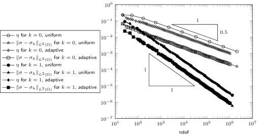
Figure 2: Errors and error estimators for the experiment on the square from Subsection 7.1.

The errors $\|\sigma-\sigma_{h}\|_{L^{2}(\Omega)}$ and error estimators $\sqrt{\lambda^{2}+\mu^{2}}$ are plotted in Figure 2 versus the degrees of freedom. The errors and error estimators show an equivalent behaviour with an overestimation factor of approximately 10. The errors and error estimators show a convergence rate of $\texttt{ndof}^{-1/2}$ for $k=0$ and of $\texttt{ndof}^{-1}$ for $k=1$ on the sequence of uniformly red-refined triangulations as well as on the sequence of triangulations generated by Algorithm 6.1. All marking steps in Algorithm 6.1 for $k=0,1$ applied the Dörfler marking ($\mu_{\ell}^{2}\leq\kappa\lambda_{\ell}^{2}$).

7.2 L-shaped domain with unknown solution for $m=2$

This subsection considers the problem

$$\Delta^{2}u=1$$

on the L-shaped domain $\Omega:=(-1,1)^{2}\setminus([0,1]\times[-1,0])$ with clamped boundary conditions $u|_{\partial\Omega}=(\partial u/\partial\nu)|_{\partial\Omega}=0$ and unknown solution. Define the right-hand side $\varphi\in H(\operatorname{div}^{2},\Omega)$ with $\operatorname{div}^{2}\varphi=1$ by

$$\varphi(x,y):=\begin{pmatrix}x^{2}/4&0\\ 0&y^{2}/4\end{pmatrix}.$$

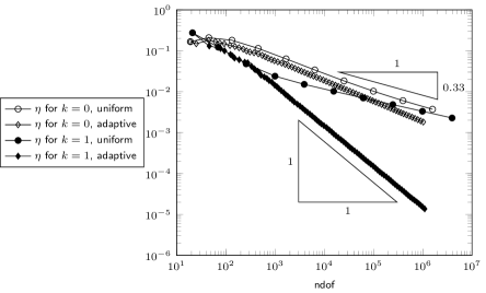
Figure 3: Error estimators for the experiment on the L-shaped domain from Subsection 7.2.

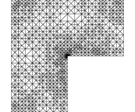
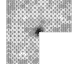
Figure 4: Adaptively refined triangulations for $k=0$ with 1096 nodes (2195 dofs) and for $k=1$ with 1077 nodes (5114 dofs) for the experiment on the L-shaped domain from Subsection 7.2.

The error estimators $\sqrt{\lambda^{2}+\mu^{2}}$ are plotted in Figure 3 versus the degrees of freedom. For uniform mesh-refinement the convergence rate of the error estimator for $k=1$ is $\texttt{ndof}^{-1/3}$. The convergence rate for $k=0$ is slightly larger, but the size of the error estimator is larger than for $k=1$. This suggests that the observed higher convergence rate is a preasymptotic effect. On the sequences of triangulations generated by Algorithm 6.1, the error estimators show the optimal convergence rates of $\texttt{ndof}^{-1/2}$ and $\texttt{ndof}^{-1}$ for $k=0$ and $k=1$, respectively. Figure 4 displays triangulations with approximately 1000 vertices generated by Algorithm 6.1 for $k=0$ and $k=1$. A stronger refinement towards the re-entrant corner is clearly visible. The marking with respect to the data-approximation ($\mu_{\ell}^{2}>\kappa\lambda_{\ell}^{2}$ in Algorithm 6.1) is only applied at the first two levels for $k=0$. All other marking steps for $k=0,1$ use the Dörfler marking ($\mu_{\ell}^{2}\leq\kappa\lambda_{\ell}^{2}$).

7.3 Square for $m=3$

In this subsection, let $\Omega=(0,1)^{2}$ be the unit square and $u\in H^{3}_{0}(\Omega)$ be defined by

$$u(x,y)=x^{3}(1-x)^{3}y^{3}(1-y)^{3}$$

with corresponding right-hand side $f:=-\Delta^{3}u$. Let $\varphi=(\varphi_{jk\ell})_{1\leq j,k,\ell\leq 2}\in H(\operatorname{div}^{3},\Omega)$ be defined by

$$\varphi_{111}(x,y) :=-\frac{1}{2}\int_{0}^{x}\int_{0}^{s}\int_{0}^{t}f(\xi,y)\,d\xi\,dt\,ds,$$ (7.1)

$$\varphi_{222}(x,y) :=-\frac{1}{2}\int_{0}^{y}\int_{0}^{s}\int_{0}^{t}f(x,\xi)\,d\xi\,dt\,ds,$$

$$\varphi_{112} :=\varphi_{121}:=\varphi_{122}:=\varphi_{211}:=\varphi_{212}:=\varphi_{221}:=0.$$

Then $-\operatorname{div}^{3}\varphi=f$ and $\varphi$ is an admissible right-hand side for (5.3).

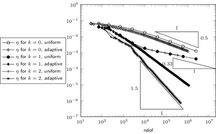
Figure 5: Errors and error estimators for the experiment on the square for $m=3$ from Subsection 7.3. The dashed lines correspond to the right-hand side generated by the solution of three successive Poisson problems.

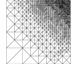
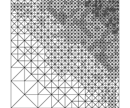
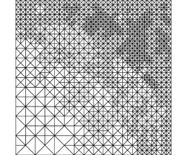
Figure 6: Adaptively refined triangulations for $k=0$ with 1460 nodes (4386 dofs), for $k=1$ with 1555 nodes (19369 dofs), and for $k=2$ with 1547 nodes (40833 dofs) for the experiment on the square from Subsection 7.3.

The errors $\|\sigma-\sigma_{h}\|_{L^{2}(\Omega)}$ and error estimators $\sqrt{\lambda^{2}+\mu^{2}}$ are plotted in Figure 5 versus the number of degrees of freedom. The errors show the optimal convergence rates of $\texttt{ndof}^{-1/2}$, $\texttt{ndof}^{-1}$, and $\texttt{ndof}^{-3/2}$ for $k=0,1,2$ for uniform refinement as well as for the sequence of triangulations generated by Algorithm 6.1. The error estimators for $k=0,1,2$ show an equivalent behaviour as the respective errors with an overestimation between 3 and 9.

Although the convergence rates are optimal, one has to consider that the $H^{3}$-seminorm of the exact solution $\|\sigma\|_{L^{2}(\Omega)}$ is approximately $2\times 10^{-2}$. That means that the relative errors for $k=1$ (resp. $k=2$) are larger than $100\%$ up to $10^{5}$ (resp. $10^{4}$) degrees of freedom and for $k=0$, they do not even reach this threshold. While the $L^{2}$ norm of the function $\sigma$ of interest is approximately $10^{-2}$, the $L^{2}$ norm of $\varphi$ (and thus $\left\|\operatorname{Curl}\alpha\right\|_{L^{2}(\Omega)}$) is approximately 80. The best-approximation result (5.4) therefore seems to suffer from the large term

$$\inf_{\beta_{h}\in Y_{h}(\mathcal{T})}\left\|\operatorname{Curl}(\alpha-\beta_{h})\right\|_{L^{2}(\Omega)}$$

on the right-hand side.

A second choice for the right-hand side $\varphi$ should indicate one possibility to decrease the error. To this end, define $\widetilde{\varphi}:=\nabla w_{3}$ with $(w_{1},w_{2},w_{3})\in H^{1}_{0}(\Omega)\times H^{1}_{0}(\Omega;\mathbb{R}^{2})\times H^{1}_{0}(\Omega;\mathbb{R}^{2\times 2})$ the solution of

$$(\nabla w_{1},\nabla v)_{L^{2}(\Omega)} =(f,v)_{L^{2}(\Omega)} \qquad\text{for all }v\in H^{1}_{0}(\Omega)$$ (7.2)

$$(\nabla w_{2},\nabla v)_{L^{2}(\Omega)} =(\nabla w_{1},v)_{L^{2}(\Omega)} \qquad\text{for all }v\in H^{1}_{0}(\Omega;\mathbb{R}^{2})$$

$$(\nabla w_{3},\nabla v)_{L^{2}(\Omega)} =(\nabla w_{2},v)_{L^{2}(\Omega)} \qquad\text{for all }v\in H^{1}_{0}(\Omega;\mathbb{R}^{2\times 2}).$$

Then $-\operatorname{div}^{3}\widetilde{\varphi}=f$ and the computations are performed with the approximation $\widetilde{\varphi}_{h}$ of $\widetilde{\varphi}$ computed by the approximation of the Poisson problems (7.2) by standard conforming FEMs of degree $k$. The errors for this right-hand side are included in Figure 5 for $k=0,1,2$ with dashed lines. The errors show the optimal convergence rates and the size of the errors are reduced by a factor between $10^{2}$ and $10^{3}$ compared to the errors for the right-hand side given by (7.1). In this situation, the error is below $100\%$ for all triangulations.

Figure 6 displays triangulations with approximately 1500 vertices generated by Algorithm 6.1 for $k=0,1,2$. Although the solution is smooth, a strong refinement towards the corner $(1,1)$ can be observed for $k=0$. For $k=1$, there is a slight refinement towards the corner $(1,1)$, while for $k=2$, the refinement is nearly uniform. Since the relative errors for $k=0,1$ are still over $100\%$ on these triangulations, the discrete solution probably do not reflect the behaviour of the exact smooth solution. However, the convergence rates are optimal and the error is slightly smaller compared with the uniform refinement. This is in agreement with Theorem 6.4.

All marking steps in Algorithm 6.1 for $k=0,1,2$ used the Dörfler marking ($\mu_{\ell}^{2}\leq\kappa\lambda_{\ell}^{2}$).

7.4 L-shaped domain for $m=3$

This section considers the problem: Find $u\in H^{3}_{0}(\Omega)$ with

$$-\Delta^{3}u=1$$

and homogeneous Dirichlet boundary conditions on the L-shaped domain $\Omega:=(-1,1)^{2}\setminus([0,1]\times[-1,0])$. Let $\varphi=(\varphi_{jk\ell})_{1\leq j,k,\ell\leq 2}\in H(\operatorname{div}^{3},\Omega)$ be defined by

$$\varphi_{111}(x,y) :=-x^{3}/12,$$

$$\varphi_{222} :=-y^{3}/12,$$

$$\varphi_{112} :=\varphi_{121}:=\varphi_{122}:=\varphi_{211}:=\varphi_{212}:=\varphi_{221}:=0$$

Then $-\operatorname{div}^{3}\varphi=1$ and $\varphi$ is an admissible right-hand side for (5.3).

Figure 7: Errors and error estimators for the experiment on the L-shaped domain for $m=3$ from Subsection 7.4.

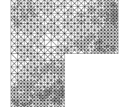
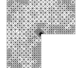
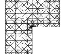
Figure 8: Adaptively refined triangulations for $k=0$ with 1118 nodes (3360 dofs), for $k=1$ with 1005 nodes (11679 dofs), and for $k=2$ with 1004 nodes (25875 dofs) for the experiment on the L-shaped domain from Subsection 7.4.

Since the exact solution is not known, only the error estimators $\sqrt{\lambda^{2}+\mu^{2}}$ are plotted in Figure 7 for $k=0,1,2$ on a sequence of uniformly red-refined triangulations and on a sequence generated by Algorithm 6.1. On the sequence of uniformly refined meshes, the error estimators for $k=1,2$ show a convergence rate of $\texttt{ndof}^{-1/3}$, while the error estimator for $k=0$ converges with rate $1/2$. However, this error estimator is of larger size than the error estimators for $k=1,2$ and it is therefore expected that the higher rate is a preasymptotic effect. Algorithm 6.1 leads to the optimal convergence rates of $\texttt{ndof}^{-1/2}$ for $k=0$, $\texttt{ndof}^{-1}$ for $k=1$, and $\texttt{ndof}^{-3/2}$ for $k=2$.

Figure 8 displays triangulations with approximately 1000 vertices generated by Algorithm 6.1 for $k=0,1,2$. The strong refinement towards the re-entrant corner is clearly visible for $k=1,2$, while for $k=0$ the refinement is quasi-uniform. This is in agreement with the observed convergence rate for $k=0$ and the interpretation that the behaviour of the exact solution is not reflected in the discrete solution up to this number of degrees of freedom. The marking with respect to the data-approximation ($\mu_{\ell}^{2}>\kappa\lambda_{\ell}^{2}$ in Algorithm 6.1) is only applied at levels 1 and 2 for $k=0$. All other marking steps for $k=0,1,2$ use the Dörfler marking ($\mu_{\ell}^{2}\leq\kappa\lambda_{\ell}^{2}$).

References

- [AF89] D. N. Arnold and R. S. Falk. A uniformly accurate finite element method for the Reissner-Mindlin plate. SIAM J. Numer. Anal., 26(6):1276–1290, 1989.
- [BBF13] D. Boffi, F. Brezzi, and M. Fortin. Mixed Finite Element Methods and Applications, volume 44 of Springer Series in Computational Mathematics. Springer, Heidelberg, 2013.
- [BD04] P. Binev and R. DeVore. Fast computation in adaptive tree approximation. Numer. Math., 97(2):193–217, 2004.
- [BDD04] P. Binev, W. Dahmen, and R. DeVore. Adaptive finite element methods with convergence rates. Numer. Math., 97(2):219–268, 2004.
- [BLN04] J. W. Barrett, S. Langdon, and R. Nürnberg. Finite element approximation of a sixth order nonlinear degenerate parabolic equation. Numer. Math., 96(3):401–434, 2004.
- [BNS07] L. Beirão da Veiga, J. Niiranen, and R. Stenberg. A posteriori error estimates for the Morley plate bending element. Numer. Math., 106(2):165–179, 2007.
- [Bre74] F. Brezzi. On the existence, uniqueness and approximation of saddle-point problems arising from Lagrangian multipliers. Rev. Française Automat. Informat. Recherche Opérationnelle Sér. Rouge, 8(R-2):129–151, 1974.
- [Bre12] S. C. Brenner. interior penalty methods. In Frontiers in Numerical Analysis—Durham 2010, volume 85 of Lect. Notes Comput. Sci. Eng., pages 79–147. Springer, Heidelberg, 2012.
- [BS08] S. C. Brenner and L. R. Scott. The Mathematical Theory of Finite Element Methods, volume 15 of Texts in Applied Mathematics. Springer Verlag, New York, Berlin, Heidelberg, 3 edition, 2008.
- [CGH14] C. Carstensen, D. Gallistl, and J. Hu. A discrete Helmholtz decomposition with Morley finite element functions and the optimality of adaptive finite element schemes. Comput. Math. Appl., 68(12):2167–2181, 2014.
- [Cia78] Ph. G. Ciarlet. The Finite Element Method for Elliptic Problems. Studies in Mathematics and its Applications, Vol. 4. North-Holland Publishing Co., Amsterdam-New York-Oxford, 1978.
- [CKNS08] J. M. Cascon, Ch. Kreuzer, R. H. Nochetto, and K. G. Siebert. Quasi-optimal convergence rate for an adaptive finite element method. SIAM J. Numer. Anal., 46(5):2524–2550, 2008.
- [CR73] M. Crouzeix and P.-A. Raviart. Conforming and nonconforming finite element methods for solving the stationary Stokes equations. I. Rev. Française Automat. Informat. Recherche Opérationnelle Sér. Rouge, 7(R-3):33–75, 1973.
- [CR15] C. Carstensen and H. Rabus. Axioms of adaptivity for separate marking. preprint, arXiv:1606.02165, 2016.
- [EGH+02] G. Engel, K. Garikipati, T. J. R. Hughes, M. G. Larson, L. Mazzei, and R. L. Taylor. Continuous/discontinuous finite element approximations of fourth-order elliptic problems in structural and continuum mechanics with applications to thin beams and plates, and strain gradient elasticity. Comput. Methods Appl. Mech. Engrg., 191(34):3669–3750, 2002.
- [Eva10] L. C. Evans. Partial Differential Equations, volume 19 of Graduate Studies in Mathematics. American Mathematical Society, Providence, RI, second edition, 2010.
- [Gal15] D. Gallistl. Stable splitting of polyharmonic operators by generalized Stokes systems. INS Preprint 1529, Institut für Numerische Simulation, Germany, 2015.
- [GN11] Th. Gudi and M. Neilan. An interior penalty method for a sixth-order elliptic equation. IMA J. Numer. Anal., 31(4):1734–1753, 2011.
- [Kin89] J. R. King. The isolation oxidation of silicon: the reaction-controlled case. SIAM J. Appl. Math., 49(4):1064–1080, 1989.
- [LM72] J.-L. Lions and E. Magenes. Non-homogeneous Boundary Value Problems and Applications. Vol. I. Die Grundlehren der mathematischen Wissenschaften, Band 181. Springer-Verlag, New York-Heidelberg, 1972.
- [Mor68] L.S.D. Morley. The triangular equilibrium element in the solution of plate bending problems. Aeronaut.Quart., 19:149–169, 1968.
- [Neč67] J. Nečas. Les Méthodes Directes en Théorie des Équations Elliptiques. Masson et Cie, Éditeurs, Paris; Academia, Éditeurs, Prague, 1967.
- [Rud76] W. Rudin. Principles of Mathematical Analysis. McGraw-Hill Book Co., New York-Auckland-Düsseldorf, third edition, 1976.
- [Sch15] M. Schedensack. A new generalization of the non-conforming FEM to higher polynomial degrees. 2015. Preprint, arXiv:1505.02044.
- [Sch16] M. Schedensack. Mixed finite element methods for linear elasticity and the Stokes equations based on the Helmholtz decomposition. ESAIM Math. Model. Numer. Anal., http://dx.doi.org/10.1051/m2an/2016024, 2016.
- [Ste08] R. Stevenson. The completion of locally refined simplicial partitions created by bisection. Math. Comp., 77(261):227–241, 2008.
- [SZ90] L. R. Scott and S. Zhang. Finite element interpolation of nonsmooth functions satisfying boundary conditions. Math. Comp., 54(190):483–493, 1990.
- [Vee14] A. Veeser. Approximating gradients with continuous piecewise polynomial functions. Foundations of Computational Mathematics, pages 1–28, 2014.
- [Ver96] R. Verfürth. A Review of a Posteriori Error Estimation and Adaptive Mesh-Refinement Techniques. Advances in numerical mathematics. Wiley, 1996.
- [WX13] M. Wang and J. Xu. Minimal finite element spaces for -th-order partial differential equations in . Math. Comp., 82(281):25–43, 2013.
- [Žen70] A. Ženíšek. Interpolation polynomials on the triangle. Numer. Math., 15:283–296, 1970.