Harnessing the Deep Net Object Models for enhancing Human Action Recognition

Abstract

In this study, the influence of objects is investigated in the scenario of human action recognition with large number of classes. We hypothesize that the objects the humans are interacting will have good say in determining the action being performed. Especially, if the objects are non-moving, such as objects appearing in the background, features such as spatio-temporal interest points, dense trajectories may fail to detect them. Hence we propose to detect objects using pre-trained object detectors in every frame statically. Trained Deep network models are used as object detectors. Information from different layers in conjunction with different encoding techniques is extensively studied to obtain the richest feature vectors. This technique is observed to yield state-of-the-art performance on HMDB51 and UCF101 datasets.

I Introduction

We deal with the problem of supervised human action recognition from unconstrained ‘real-world’ videos. The objective is to determine an action (one per time instance) performed in a given video. In the scenario where large number of action classes are present such as HMDB51 [1] and UCF101 [2] with 51 and 101 classes respectively, five Major categories [1] can be classified as shown in Table I. The major discriminating information between two categories such as (1) and (2) is the objects with which the human are interacting! The discriminating information for action classes within a category such as in (4) – Shoot ball, Shoot bow, Shoot gun – is the objects information. Further, if the objects were to be non-moving, such as gun, bow, they would not be detected by the spatio-temporal interest points or trajectories.

To overcome these limitations, we use Convolution Neural Networks (CNN) pre-trained on the Imagenet [3] 1000 object categories. CNNs are very efficient to train, faster to apply and better in accuracy as objects detectors [4]. These deep nets learn the invariant representation and object classification result simultaneously by back-propagating information, through stacked convolution and pooling layers, with the aid of a large number of labelled examples.

TABLE I: Broader Categories in Human Action Recognition

Index	Category	Actions in the HMDB51 dataset
1	General facial actions	Smile, Laugh, Chew, Talk
2	Facial actions with object manipulation	Smoke, Eat, Drink
3	General body movements	Cartwheel, Clap hands, Climb, Climb stairs, Dive, Backhand flip, Fall on the floor, Handstand,
		Jump, Pull up, Push up, Run, Sit down, Sit up, Somersault, Stand up, Turn, Walk, Wave
4	Body movements with object interaction	Brush hair, Catch, Draw sword, Dribble, Golf, Hit something,Kick ball, Pick, Pour, Push something,
		Ride bike, Ride horse, Shoot ball, Shoot bow, Shoot gun, Swing baseball bat, Sword exercise, Throw
5	Body movements for human interaction	Fencing, Hug, Kick someone, Kiss, Punch, Shake hands, Sword fight

In this context, we investigate the following questions

1. What is the influence of objects in human action recognition ?

2. Generalization capabilities of the constructed object feature vectors

We study and present our results on the large-scale action datasets HMDB51 and UCF101 containing at least 51-101 different action classes.

In the remainder of the paper, Section II contains a review of the related works. Section III describes the framework and details the local feature descriptors, codebook generation, object detectors, different feature encoding techniques, classifier and datasets. Section IV presents and discusses the results obtained on the benchmark datasets. Finally, conclusions are drawn in Section V.

II Related Literature

The influence of objects in human action recognition has begun with recent works [5] and [6]. Jain et al. [5] conduct an empirical study on the benefit of encoding 15,000 object categories for action recognition. They show that objects matter for actions, and are often semantically relevant as well. And,when objects are combined with motion, improve the state-of-the-art for both action classification and localization. They train 15,000 object classifiers from the Imagenet [3] with a deep convolutional neural network [4] and use their pooled responses as a video representation for action classification and localization. However, they utilized only the final output responses (softmax probability scores) of Deep net models as features. Cai et al. [6] utilized intermediate-level Deep net model outputs (Fc6) as features along with low level features and 1418 Semantic Concept detectors trained from ConceptsWeb [7]. ConceptsWeb consists of half a million images downloaded from the web, manually annotated and organized in a hierarchical faceted taxonomy. Further, they fuse these features through extensive experimental evaluations and show improved action classification performance. Xu et al. [8] investigated extensively intermediate-level Deep net model outputs (Pool5, Fc6, Fc7) in conjunction with different feature encoding techniques. However, their Deep net models were trained for action recognition, not object detection.

III Overall Framework and Background

The overall layout of our proposed framework is shown in Fig. 1. Firstly, interest points – trajectories of moving objects – are detected. Local descriptors are computed around these detected interest points. Gaussian Mixture Modelling is applied and Fisher vectors are generated. In a parallel channel, objects are detected in each frame statically, using pre-trained object detectors from Imagenet. Feature vectors are constructed, using different encoding, from different layers of the pre-trained object detectors. These feature vectors are concatenated to the Fisher vector to learn a classifier (for each action class detection). The details of each stage are discussed in following sections.

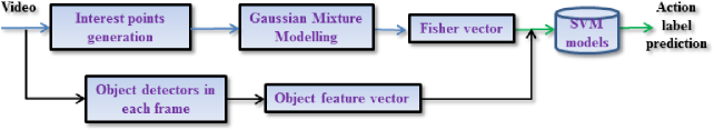
Figure 1: Overall Framework

III-A Spatio-Temporal Interest Points

In their seminal work, Laptev et al. [9] proposed the usage of Harris 3D corners as an extension of traditional (2D) Harris corner points for spatio-temporal analysis and action recognition. These interest points are local maxima of a function of space-time gradients. They compute a spatio-temporal second-moment matrix at each video point in different spatio-temporal scales. This matrix essentially captures space-time gradients. The interest points are obtained as local maxima of a function of this second-moment matrix. We use the original implementation with standard parameter settings. These points are extracted at multiple scales based on a regular sampling of spatial and temporal scale values. They are defined in 5 dimensions $(x,y,t,\sigma,\tau)$, where $x$, $y$ and $t$ are spatial and temporal axes, resp., while $\sigma$ and $\tau$ are the spatial and temporal scales, respectively. Local descriptors histograms of oriented gradients (HOG) and histograms of optic flow (HOF) are computed around the detected interest points.

III-B Dense Trajectories

Wang et al. [10] proposed dense trajectories to model human actions. Interest points were sampled at uniform intervals in space and time, and tracked based on displacement information from a dense optical flow field. Improved dense trajectories (iDT) [11] are an improved version of the dense trajectories obtained by estimating the camera motion. Wang and Schmid [11] use a human body detector to separate motion stemming from humans movements from camera motion. The estimate is also used to cancel out possible camera motion from the optical flow. For trajectories of moving objects, we compute these improved dense trajectories. In our experiments, we only use the online version [11] of camera motion compensated improved trajectories, without any human body detector. The local descriptors computed on these trajectories are HOG, HOF, motion boundary histograms (MBH) and trajectory shape.

III-C Multi-Skip Feature Stacking

Generally, action feature extractors such as STIP, iDT, involve differential operators, which act as high-pass filters and tend to attenuate low frequency action information. This attenuation introduces bias to the resulting features and generates ill-conditioned feature matrices. To overcome this limitation, Lan et al. [12] proposed Multi-Skip Feature Stacking (MIFS), which stacks features extracted using a family of differential filters parameterized with multiple time skips ($L$) and encodes shift-invariance into the frequency space. MIFS compensates for information lost from using differential operators by recapturing information at coarse scales. This recaptured information matches actions at different speeds and ranges of motion.

MIFS on improved dense trajectories are used in the current experiments. On the choice of $L$, Lan et al. report that having one or two more scales than the original scale is enough to recover most of lost information due to the differential operations. However, higher scale features become less reliable due to the increasing difficulty in optical flow estimation and tracking. Hence, $L=3$ is finalized.

III-D Object Detectors

We utilize existing deep learning framework for computing object detection scores from each video frame. The open source MatConvNet [13] implementation based on the deep convolutional neural network architecture by Simonyan and Zisserman [14] is used in all our experiments. We take the ImageNet model, Imagenet-vgg-verydeep-16 , trained on previous ILSVRC image classification tasks to compute 1000 object detection responses from each frame. We set the network input to the raw RGB values of the frames, resized to $224\times 224$ pixels, and the values are forward propagated through 5 convolutional layers (i.e., pooling and ReLU non-linearities) and 3 fully-connected layers (i.e., to determine its final neuron activities). The architecture is shown in Figure 2.

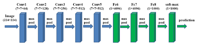
Figure 2: Architecture of vgg16

In Imagenet CNNs, different layers of deep networks can express different information. The fully-connected layer (softmax probabilities) usually denotes high-level concepts. Deeper convolutional layers (Fc6, Fc7) contain global expressions such as object and scene, while shallower convolutional layers contain local characteristics of the image like lines, edges. Jain et al. [5] use fully-connected layers for action recognition; other layers like pooling layer [8], convolutional layers [15] are also extracted and utilized. All these three levels of information are investigated thoroughly in this study and discussed below

1. Objects1K: This is based on final layer (softmax probabilities). A probability score in the range 0-1 is assigned to each of the 1000 object categories, and totalling to 1. The $N(=1000)$ dimensional vector of object attribute scores $(S(i);i=1...N)$ is computed for each frame. These vectors are then simply averaged across the frame to yield

   $$\textbf{Objects1K}=\dfrac{1}{F}\sum S_{xf}$$ (1)

   where $F$ is the number of frames in video $x$, $S_{xf}$ is the object vector representation per frame. Jain et al. [5] used the same strategy – computing scores for 15K objects.

2. Fc6, Fc7 layers: The activations of the neurons in the intermediate hidden layers – Fc6, Fc7 – can be used as strong features because they contain much richer and more complex representations. Each one of them is of the $4096D$ dimensions. The response from each frame are average pooled [6], VLAD and Fisher encoded [8]. Details of VLAD and FV encoding are presented in Section III-E. As the dimensions of descriptors is very high, PCA is applied to reduce to 256D before applying VLAD/Fisher encoding.

3. Latent Concept Descriptors (LSD): Compared to the fully-connected layers, pool5 contains spatial information. The feature dimension of pool5 is $a\times a\times M$, where $a$ is the size of filtered images of the last pooling layer and $M$ is the number of convolutional filters in the last convolutional layer (in our case based on the VGG Imagenet model [14], $a=7$ and $M=512$). Flattening pool5 into a vector will yield to very high dimensional features, which will induce heavy computational cost and instability problems [16]. However, the convolutional filters can be regarded as generalized linear classifiers on the underlying data patches, and each convolutional filter corresponds to a latent concept. Xu et al. [8] formulate the general features from pool5 as the vectors of latent concept descriptors, in which each dimension of the latent concept descriptors represents the response of the specific latent concept. Each filter in the last convolutional layer is independent from other filters. The response of the filter is the prediction of the linear classifier on the convolutional location for the corresponding latent concept. In that way, pool5 layer of size $a\times a\times M$ is converted into $a^{2}$ latent concept descriptors with $M$ dimensions. Each latent concept descriptor represents the responses from the $M$ filters for a specific pooling location. In this case, each frame contains $a^{2}$ descriptors instead of one descriptor for the frame. After the latent concept descriptors for all the frames in a video are obtained, PCA is applied to reduce the descriptor dimensions to half (i.e. 256). Then an encoding method – VLAD and FV – is applied to generate the feature vector.

III-E Feature Encoding

After the descriptors are obtained, either from low-level features or from CNNs, they have to be encoded to yield the feature vector for each video. Two types of encoding popular in practise in this domain – Vector of Locally Aggregated Descriptors (VLAD) and Fisher Vector (FV) – are reviewed and applied in this study. These techniques are based on a measure determining how much a descriptor belongs to a particular (assigned) visual word.

• Vector of Locally Aggregated Descriptors (VLAD)

  In this type of encoding, the difference between the descriptors and the closest visual word is collected as residual vectors. K coarse centers ${mu_{1},mu_{2},...mu_{K}}$ are generated by K-means clustering from a randomnly selected (100,000) descriptors. For each coarse center dimension $d$ (dimension of the local feature descriptor, $x_{i}$), a sub-vector $v^{i}$ is obtained by accumulating the residual vectors as

  $$v^{i}=\sideset{}{}{\sum}_{x:q(x)=\mu_{i}}x-\mu$$ (2)

  The obtained sub-vectors are concatenated to yield a $D$-dimensional vector, where $D=k\times d$. Then intra-normalization [17] is applied. Further, a two-stage normalisation is applied. Firstly, the ‘power-law normalisation’ [18] is applied. It is a component-wise non-linear operation. Each component $v_{j},j=1$ to $D$ is modified as

  $$v_{j}={|v_{j}|}^{\alpha}\times sign(v_{j}),$$ (3)

  where $\alpha$ is a parameter such that $\alpha\leq 1$. In all experiments, $k=256$ and $\alpha=0.2$. Secondly, the vector is $L_{2}$-normalised as $v=\frac{v}{||v||}$ to yield the VLAD vector.

• Fisher Vector Encoding

  In this technique, a Gaussian Mixture Model (GMM) is fitted to a randomly selected (250,000) descriptors from the training set. Let the parameters obtained from the GMM fitting be defined as $\theta=(\mu_{k},\sum_{k},\pi_{k};k=1,2,...,K)$ where $\mu_{k},\sum_{k}$ and $\pi_{k}$ are the mean, covariance and prior probability of each distribution, respectively. The GMM associates each descriptor $X_{i}$ to a mode $k$ in the mixture with a strength given by the posterior probability

  $$q_{ik}=\dfrac{exp[-\dfrac{1}{2}(X_{i}-\mu_{k})^{T}\sum_{k}^{-1}(X_{i}-\mu_{k})]}{\sum_{t=1}^{K}exp[-\dfrac{1}{2}(X_{i}-\mu_{t})^{T}\sum_{k}^{-1}(X_{i}-\mu_{t})]}$$ (4)

  The mean ($u_{jk}$) and deviation vectors ($v_{jk}$) for each mode k are computed as

  $$u_{jk}=\dfrac{1}{N\sqrt{\pi_{k}}}\sum_{i=1}^{N}q_{ik}\frac{x_{ji}-\mu_{jk}}{\sigma_{jk}}$$ (5)

  $$v_{jk}=\dfrac{1}{N\sqrt{2\pi_{k}}}\sum_{i=1}^{N}q_{ik}[(\frac{x_{ji}-\mu_{jk}}{\sigma_{jk}})^{2}-1]$$ (6)

  where $j=1,2,...,D$ spans the local descriptor vector dimensions. The FV is then obtained by concatenating the vectors ($u_{jk}$) and ($v_{jk}$) for each of the K modes in the Gaussian mixtures. Similar to VLAD encoding, the FV is also finally normalized by the ‘power-law normalisation’ and $L_{2}$-normalisation. We concatenate all the Fisher Vectors (of different descriptors) to yield the final feature vector for a given video.

For classification we use the final feature vectors and linear SVM [19]. We apply the one-versus-all approach in all the cases and select the class with the highest score.

III-F Datasets

We applied our proposed technique on three benchmark datasets: HMDB51 [1] and UCF101 [2]. HMDB51 contains 51 actions categories. Digitised movies, public databases such as the Prelinger archive, videos from YouTube and Google videos were used to create this dataset. For evaluation purposes, three distinct training and testing splits were specified in the dataset. These splits were built to ensure that clips from the same video were not used for both training and testing. For each action category in a split, 70 training and 30 testing clips indices were fixed so that they fulfil the 70/30 balance for each meta tag. UCF101 data set consists of 101 action categories, collected from realistic action videos, e.g. from YouTube. Three train-test splits were provided for consistency in reporting performance.

TABLE II: Performance of Objects

Index	Feature type/technique	Dimesnions	HMDB51	UCF101
i	Objects1K	1000	26.0%	58.3%
ii	Fc6 Average pooling	4096	35.1%	70.5%
	Fc7 Average pooling	4096	32.8%	65.1%
	Fc6 + Fc7 Average pooling	8192	35.8%	71.7%
iii	Fc6 Fisher vector	130K	24.4%	58.9%
	Fc7 Fisher vector	130K	23.9%	58.9%
	Fc6 + Fc7 Fisher vector	130K	24.6%	59.1%
iv	Fc6 VLAD	65K	22.7%	53.5%
	Fc7 VLAD	65K	28.0%	53.8%
	Fc6 + Fc7 VLAD	65K	22.0%	53.8%
v	LSD Fisher vector	130K	37.8%	71.9%
	LSD VLAD	65K	41.9%	78.2%
vi	15000 objects scores aggregated [5]	15K	38.9%	65.6%
vii	1000 objects Fc6 average pooling [6]	4096	33.05%	65.88%

IV Results and Discussions

We now present the results obtained by applying the techniques discussed earlier. In each Table, the highest recognition rates observed are highlighted.

IV-A What is the influence of objects in human action recognition ?

The results obtained by applying CNN models as object detectors are shown in Table II. Information from different layers of the Deep net models are encoded using different techniques. It is observed that (pool5 layer outputs with VLAD encoding technique performed best.

TABLE III: Performance of Objects in combination with other feature representations

Index	Feature type/technique	HMDB51	UCF101
i	Fisher vector (FV) from STIP [20]	37.9%	69.4%
ii	STIP + Objects1K	43.1%	75.6%
iii	STIP + (Fc6+Fc7) average pooling	42.7%	80.6%
iv	STIP + LSD Fisher	47.5%	81.1%
v	STIP + LSD VLAD	50.5%	84.5%
vi	FV from Improved dense trajectories (iDT)	55.9% [11]	84.8%[21]
vii	iDT + Objects1K	59.5%	87.0%
viii	iDT + (Fc6+Fc7) average pooling	60.3%	89.4%
ix	iDT + LSD Fisher	60.0%	89.0%
x	iDT + LSD VLAD	61.7%	90.8%
xi	Multi-Skip ($L=3$) [12]	65.1%	89.1%
xii	Multi-Skip + Objects1K	66.5%	89.3%
xiii	Multi-Skip + (Fc6+Fc7) average pooling	66.6%	91.0%
xiv	Multi-Skip + LSD Fisher	66.4%	90.6%
xv	Multi-Skip + LSD VLAD	68.0%	91.9%

IV-B Generalization capabilities of the constructed object feature vectors

The three best performing features observed in Table II were found to be LSD VLAD, LSD Fisher and (Fc6+Fc7) average pooling. The influence of these features on three different state-of-the-art feature representations are presented in Table III. The constructed object feature vectors are complimentary with all the three different kinds of feature representations. This shows that Deep net features are not over-fitted to some databases; yet have generalization capacity. An improvement of 12-14.9% (absolute), 5.8% (absolute) and 2.9%(absolute) has been observed in STIP (Table III v), iDT (Table III x) and Multi-Skip (iDT) feature representations (Table III xv) respectively.

TABLE IV: Comparison with other techniques

Approach	Brief description	HMDB51	UCF101
Improved dense trajectories (iDT)	Fisher vector (FV)	55.9% [11]	84.8%[21]
Best of Proposed technique	Multi-Skip (iDT) + LSD VLAD	68.0%	91.9%
Jain et al. 2015 [5]	15K Objects prob scores + iDT	61.4%	88.5%
Cai et al. 2015 [6]	Objects Fc6 + iDT + semantic concepts	62.9%	89.6%
Wang et al. 2015 [22]	Trajectory pooled Descriptors + iDT	65.9%	91.5%
Miao et al. 2015 [23]	Temporal variance analysis on iDT	66.4%	90.2%
Lan 2015 [24]	MIFS(iDT) + ConvISA + MIR	67.0%	90.2%

IV-C Comparison with state-of-the-art

We compare our results with recent works from 2015 only (as their performances are already better than most of the earlier works). The closest works on Deep net based objects influence are by Jain et al. [5] and Cai et al. [6]. However, they did not extensively focus on tapping the information from the Deep net models. Jain et al. used only final output layer (softmax probability scores) of the Deep net models. pool5 layer from Deep net models of 15,000 object detectors might significantly improve the performance. Cai et al. used only Fc6 information with average pooling. However, pool5 layer in conjunction with their Semantic web concepts detectors might also yield improved results. We would like to investigate them in future.

Other latest works, but not focused exclusively on objects are as follows. Wang et al. [22] learn discriminative convolutional feature maps and conduct trajectory-constrained pooling to aggregate these convolutional features into effective descriptors called as trajectory-pooled deep convolutional descriptor (TDD). Fisher vectors are then constructed from these TDDs. Miao et al. [23] proposed temporal variance analysis (TVA) as a generalization to better utilize temporal information. TVA learns a linear transformation matrix that projects multidimensional temporal data to temporal components with temporal variance. By mimicking the function of visual cortex (V1) cells, appearance and motion information are obtained by slow and fast features from gray videos using slow and fast filters, respectively. Additional motion features are extracted from optical flows. In this way, slow features encode velocity information, and fast features encode acceleration information. By using parts of fast filters as slow filters and vice versa, the hybrid slim filter is proposed to improve both slow and fast feature extraction. Finally, they separately encode extracted local features with different temporal variances and concatenate all the encoded features as final features. Lan [24] used four complementary methods to improve the performance of action recognition by unsupervised learning from iDT features. Initially, MIFS enhanced iDT features are used to learn motion descriptors using Stacked Convolutional Independent Subspace Analysis (ConvISA) [25]. Then, spatio-temporal information is incorporated into the learned descriptors by augmenting with normalized spatio-temporal location information. Finally, the relationship among action classes is captured by a Multi-class Iterative Re-ranking (MIR) method [26] that exploits the relationship among classes. The best Deep net based object information investigated in this paper may also be turn out to be complimentary with these latest methods. This will be investigated in the future work.

V Conclusions

In this study, the influence of objects using Deep net models was investigated thoroughly. Information from different layers of the the Deep net models was extensively investigated in conjunction with different feature encoding techniques. Information from pool5 with VLAD encoding technique was found to be very rich and complementary to different types of low-level feature representations; supporting its generalization capacity. Competitive state-of-the-art performances are achieved on two benchmark datasets.

References

- [1] H. Kuehne, H. Jhuang, E. Garrote, T. Poggio, and T. Serre, “HMDB: A large video database for human motion recognition,” in International Conference on Computer Vision (ICCV), 2011.
- [2] K. Soomro, A. R. Zamir, and M. Shah, “UCF101: A Dataset of 101 Human Action Classes from Videos in the Wild,” in CRCV-TR-12-01, November 2012.
- [3] J. Deng, W. Dong, R. Socher, L.-J. Li, K. Li, and L. Fei-Fei, “Imagenet: A large-scale hierarchical image database,” in IEEE Conference on Computer Vision and Pattern Recognition (CVPR), pp. 248–255, June 2009.
- [4] A. Krizhevsky, I. Sutskever, and G. E. Hinton, “Imagenet classification with deep convolutional neural networks,” in Advances in Neural Information Processing Systems (NIPS) 25 (F. Pereira, C. Burges, L. Bottou, and K. Weinberger, eds.), pp. 1097–1105, 2012.
- [5] M. Jain, J. van Gemert, and C. Snoek, “What do 15,000 object categories tell us about classifying and localizing actions?,” in IEEE Conference on Computer Vision and Pattern Recognition (CVPR), pp. 46–55, June 2015.
- [6] J. Cai, M. Merler, S. Pankanti, and Q. Tian, “Heterogeneous semantic level features fusion for action recognition,” in Proceedings of the 5th ACM International Conference on Multimedia Retrieval (ICMR), pp. 307–314, 2015.
- [7] M. Merler, B. Huang, L. Xie, G. Hua, and A. Natsev, “Semantic model vectors for complex video event recognition,” IEEE Transactions on Multimedia, vol. 14, pp. 88–101, Feb 2012.
- [8] Z. Xu, Y. Yang, and A. G. Hauptmann, “A discriminative cnn video representation for event detection,” in IEEE Conference on Computer Vision and Pattern Recognition (CVPR), pp. 1798–1807, 2015.
- [9] I. Laptev and T. Lindeberg, “Space-Time Interest Points,” in International Conference on Computer Vision (ICCV), pp. 432–439, Oct 2003.
- [10] H. Wang, A. Kläser, C. Schmid, and C.-L. Liu, “Action recognition by dense trajectories,” in IEEE Conference on Computer Vision and Pattern Recognition (CVPR), 2011.
- [11] H. Wang and C. Schmid, “Action Recognition with Improved Trajectories,” in Intenational Conference on Computer Vision (ICCV), 2013.
- [12] Z.-Z. Lan, M. Lin, X. Li, A. G. Hauptmann, and B. Raj, “Beyond gaussian pyramid: Multi-skip feature stacking for action recognition.,” in IEEE Conference on Computer Vision and Pattern Recognition (CVPR), pp. 204–212, 2015.
- [13] A. Vedaldi and K. Lenc, “Matconvnet – convolutional neural networks for matlab,”
- [14] K. Simonyan and A. Zisserman, “Very deep convolutional networks for large-scale image recognition,” CoRR, vol. abs/1409.1556, 2014.
- [15] L. Liu, C. Shen, and A. van den Hengel, “The treasure beneath convolutional layers: cross convolutional layer pooling for image classification,” in IEEE Conference on Computer Vision and Pattern Recognition (CVPR), 2015.
- [16] M. Douze, J. Revaud, C. Schmid, and H. Jegou, “Stable hyper-pooling and query expansion for event detection,” in IEEE International Conference on Computer Vision (ICCV), pp. 1825–1832, Dec 2013.
- [17] R. Arandjelović and A. Zisserman, “All about VLAD,” in IEEE Conference on Computer Vision and Pattern Recognition (CVPR), 2013.
- [18] F. Perronnin, J. Sánchez, and T. Mensink, “Improving the Fisher kernel for large-scale image classification,” in European Conference on Computer Vision (ECCV), 2010.
- [19] R.-E. Fan, K.-W. Chang, C.-J. Hsieh, X.-R. Wang, and C.-J. Lin, “LIBLINEAR: A library for large linear classification,” Journal of Machine Learning Research, vol. 9, pp. 1871–1874, 2008.
- [20] O. V. R. Murthy and R. Goecke, “The Influence of Temporal Information on Human Action Recognition with Large Number of Classes,” in International Conference on Digital Image Computing: Techniques and Applications (DICTA), 2014.
- [21] H. Wang and C. Schmid, “LEAR-INRIA submission for the THUMOS workshop,” in THUMOS:ICCV Challenge on Action Recognition with a Large Number of Classes, Winner, 2013.
- [22] L. Wang, Y. Qiao, and X. Tang, “Action recognition with trajectory-pooled deep-convolutional descriptors.,” in IEEE Conference on Computer Vision and Pattern Recognition (CVPR), pp. 4305–4314, 2015.
- [23] J. Miao, X. Xu, S. Qiu, C. Qing, and D. Tao, “Temporal variance analysis for action recognition,” IEEE Transactions on Image Processing, vol. 24, pp. 5904–5915, Dec 2015.
- [24] Z. Lan, “Learn to recognize actions through neural networks,” in Proceedings of the 23rd ACM International Conference on Multimedia, pp. 657–660, 2015.
- [25] Q. Le, W. Zou, S. Yeung, and A. Ng, “Learning hierarchical invariant spatio-temporal features for action recognition with independent subspace analysis,” in IEEE Conference on Computer Vision and Pattern Recognition (CVPR),, pp. 3361–3368, June 2011.
- [26] M. Hoai and A. Zisserman, “Improving human action recognition using score distribution and ranking,” in Asian Conference on Computer Vision (ACCV), pp. 3–20, 2014.