Graphene Electrodynamics in the presence of the Extrinsic Spin Hall Effect

Abstract

We extend the electrodynamics of two dimensional electron gases to account for the extrinsic spin Hall effect (SHE). The theory is applied to doped graphene decorated with a random distribution of absorbates that induce spin-orbit coupling (SOC) by proximity. The formalism extends previous semiclassical treatments of the SHE to the non-local dynamical regime. Within a particle-number conserving approximation, we compute the conductivity, dielectric function, and spin Hall angle in the small frequency and wave vector limit. The spin Hall angle is found to decrease with frequency and wave number, but it remains comparable to its zero-frequency value around the frequency corresponding to the Drude peak. The plasmon dispersion and linewidth are also obtained. The extrinsic SHE affects the plasmon dispersion in the long wavelength limit, but not at large values of the wave number. This result suggests an explanation for the rather similar plasmonic response measured in exfoliated graphene, which does not exhibit the SHE, and graphene grown by chemical vapor deposition, for which a large SHE has been recently reported. Our theory also lays the foundation for future experimental searches of SOC effects in the electrodynamic response of two-dimensional electron gases with SOC disorder.

I Introduction

A number of ground-breaking experiments have recently explored the physics of plasmons in doped Dirac materials like graphene and topological insulators.Stauber (2014); Ju et al. (2011); Di Pietro et al. (2013); Grigorenko et al. (2012); Chen et al. (2012) One major difference between these two kinds of Dirac materials is the strength of the spin-orbit coupling (SOC) in their band structure. Whilst SOC is substantial in the band structure of topological insulators, it has been rightly dismissed in graphene as negligible due to the lightness of carbon. Huertas-Hernando et al. (2006); Min et al. (2006)

Nevertheless, despite of the negligible SOC in its band structure, it has been recently observed that the spin Hall effect (SHE) can occur in graphene decorated with absorbates such as hydrogen, Balakrishnan et al. (2013) and in graphene devices prepared by chemical vapor deposition (CVD), Balakrishnan et al. (2014) which contain residual metallic clusters. From the theoretical point of view, the existence of a (proximity-induced) SOC in graphene is also expected from first-principles and tight-binding calculations. Weeks et al. (2011); Brey ; Jiang et al. (2012) However, the experimental situation remains rather controversial, Wang et al. (2015); Kaverzin and van Wees (2015) and in this context, deeper theoretical studies of decorated graphene are, in our opinion, more than necessary.

A direct experimental consequence of the SOC disorder is the SHE by which an applied electric field induces a transverse spin current. Sinova et al. (2015); Dyakonov and Perel (1971); Hirsch (1999); Zhang (2000); Vignale (2010) The figure of merit of the SHE is the spin Hall angle, $\Theta_{\mathrm{SH}}$ which measures the fraction of the (longitudinal) charge current that is converted into a (transverse) spin current. In Ref. Balakrishnan et al., 2014, a large value of $\Theta_{\mathrm{SH}}\sim 0.1$ was reported, which makes CVD graphene a material comparable to platinum, a reference material in the field of metallic spintronics. Sinova et al. (2015) In this field, over the last decade, the SHE has attracted increasing theoretical Schliemann (2006); Castro Neto and Guinea (2009); Ferreira et al. (2014) and experimental Kato et al. (2004); Wunderlich et al. (2005); Seki et al. (2008); Balakrishnan et al. (2014, 2013) attention, and the most recent experimental discoveries may point the way toward a new class of graphene-based spintronic devices.Liu et al. (2011, 2012)

This paper examines corrections to electrodynamics arising from extrinsic SHE. The latter is known to occur in materials through essentially two kinds of microscopic mechanisms, namely side-jump and skew scattering.Nagaosa et al. (2010) In the doped regime, the large SHE observed in adatom decorated and CVD graphene Balakrishnan et al. (2014, 2013); Jiang et al. (2012); Gmitra et al. (2013); Irmer et al. (2015) can be attributed mainly to skew-scattering, since the total adatom coverage is typically very dilute and the side-jump contribution to the SHE is subleading in this regime. Balakrishnan et al. (2014); Sinova and MacDonald (2008); Sinova et al. (2015) The skew-scattering is strongly enhanced by the occurrence, in the neighborhood of the Dirac point, of scattering resonances caused by adatoms and other impurities. Ferreira et al. (2014); Balakrishnan et al. (2014)

In earlier work that analyzed the electrodynamic response of doped graphene by focusing on the effects of disorder, skew-scattering effects have been neglected, to the best of our knowledge. For instance, the recent analysis by Principi et al. examined the effects of disorder on graphene plasmons, Principi et al. (2013) but did not take into account the losses and other effects that may arise from SOC disorder. From a theoretical point of view, it can argued that a description neglecting the extrinsic SHE is substantially incomplete. This is because a sizable fraction of the oscillatory electric current generated by the plasmon is converted into a spin current by the SHE. Such a scenario is plausible because, in the long wavelength limit, the plasmon frequency in a two dimensional electron gas reaches arbitrarily low frequencies (i.e. the plasmon dispersion is $\omega_{p}(q)\sim\sqrt{q}$, where $q$ is the wave number). Therefore, we can approximately rely on the DC value of the spin Hall angle to estimate the charge to spin current conversion. On the other hand, it can be also argued that spin currents are charge neutral and, as a consequence, they should not modify the electrodynamic response of the system. Below we shall see that, although the latter expectation is sensible, the physics is more subtle and electrodynamics is indeed modified by the SHE.

In addition, beyond the low frequency regime, where the stationary (DC) theory of the SHE may be approximately valid, a theory capable of accounting for the full frequency dependence of the spin Hall angle needs to be formulated. Previous theoretical treaments of extrinsic SHE in graphene Ferreira et al. (2014); Balakrishnan et al. (2014); Yang et al. have focused on DC transport properties. However, the AC regime remains unexplored. Such a task is undertaken in this work, focusing on the case of doped graphene. With minor modifications, our theory can also be applied to other types of two-dimensional electron or hole gases with SOC disorder. Therefore, studies like the present one, may one day allow for spin-current generation in decorated graphene by means of plasmon excitation, a possibility which has been recently considered in the spintronics literature. Uchida et al. (2015)

Similar to Refs. Ferreira et al., 2014; Yang et al., , we consider a single layer of doped graphene decorated with (clusters of) absorbates which induce SOC by proximity. Our analysis relies on the semi-classical Boltzmann transport equation (BTE) in the dilute-impurity limit. Using a general form of the single-impurity $T$-matrix, Ferreira et al. (2014); Yang et al. we solve the time-dependent linearized BTE within a particle-conserving approximation. Mermin (1970) We find that in the presence of SOC disorder, the collision integral of the BTE contains two different contributions: (i) a conventional momentum (Drude) relaxation term, and (ii) an effective Lorentz force arising from the skew scattering with SOC disorder. From the solution of the BTE, we derive a generalized Ohm’s law in the AC regime, as well as the dynamic nonlocal charge conductivity, dielectric function, and the AC spin Hall angle.

Our theory applies to the THz regime, which corresponds to the typical plasma frequency for (moderately) doped graphene.Ju et al. (2011) The excitations in this frequency regime are dominated by the contribution of the $\pi$-band electrons, which are strongly hybridized with the outer shell electrons of the absorbates. As a result of this hybridization, the SOC disorder is induced. Therefore, our present theory does not apply to visible or higher frequencies for which electronic excitations localized in the absorbates that decorate graphene can be important. Furthermore, our theory does not apply to devices in which metallic nano-particles are deposited on top of graphene covered by a dielectric layer. In such devices, the coupling between the nanoparticles and graphene is essentially capacitive (as the insulating layer strongly or completely suppresses the hybridization of the nanoparticles with the graphene $\pi$-band), and therefore there is no proximity-induced SOC.

In order to obtain the plasmon dispersion and linewidth, we numerically find the zeros of the dielectric function in the complex frequency plane. Generally speaking, disorder has two major known effects on the plasmon properties. First, it contributes to the linewidth (i.e. imaginary part of the plasmon frequency), making the plasmon lossier. Principi et al. (2013) Second, it “softens” the plasmon dispersion by reducing the plasma frequency $\omega_{p}(q)$ relative to the clean system for each value of $q$. Thus, in the presence of disorder, the plasmon frequency vanishes at a cutoff wave number $q_{c}$. Similar softening has been previously predicted in disordered two-dimensional (2D) electron gasesGiuliani and Quinn (1984) and spin-polarized graphene. Agarwal et al. (2014) We find that SOC disorder reduces the plasmon linewidth and it modifies the plasmon softening by reducing the softening at low wave numbers and increasing it at large wave numbers, relative to the case of purely scalar disorder. These effects are relatively modest; the shifts in plasmon frequency, for instance, are of order 1% at experimentally realistic frequencies and SOC disorder strengths. We believe that this may explain why exfoliated Fei et al. (2012) and CVD graphene Chen et al. (2012) have been experimentally found to exhibit a similar plasmonic response, despite the rather large SHE effect recently observed in CVD graphene. Balakrishnan et al. (2014)

The rest of the article is organized as follows. In Sec. II, we summarize the most important results of the article, namely the AC generalization of the Ohm’s law in the presence of SOC disorder. The effect of SOC disorder on the plasmon dispersion and lifetime is also discussed in Sec. II, together with the long wavelength limit of the conductivity, dielectric function, and spin Hall angle. In Sec. III, we provide the details of the derivation of the results described in Sec. II. We close the article with a summary and an outlook in Sec. IV. The most technical parts of these derivations have been relegated to the Appendices. Throughout, we work in units where $\hbar=1$.

II Results

In this section, we summarize the main results of this work and discuss some of their experimental consequences. The derivations for the equations presented here are given in the following sections, whist the most technical details have been relegated to the Appendices. We begin by introducing a generalized Ohm’s law which relates the charge and spin currents. Hence, the form of AC charge conductivity, dielectric function, and spin Hall angle follow. The modified plasmon dispersion and linewidth, as well as the conductivity in the optical limit are also discussed in this section.

II.1 Generalized Ohm’s law

In graphene with extrinsic SOC, we find the following generalized AC Ohm’s law:

$$\bm{J}_{c}(q,\omega) =\sigma_{m}(q,\omega)\left[\bm{E}(q,\omega)-\rho_{ss}\bm{J}_{s}(q,\omega)\times\bm{\hat{z}}\right],$$ (1)

$$\bm{J}_{s}(q,\omega) =\Theta_{\mathrm{SH}}(q,\omega)\>\bm{J}_{c}(q,\omega)\times\bm{\hat{z}}.$$ (2)

Here $\bm{E}(q,\omega)$ is the electric field, $\bm{J}_{c}(q,\omega)$ is the charge current density, $\bm{J}_{s}(q,\omega)$ is the transverse spin current density, and $q$ and $\omega$ are the wave-number and frequency respectively; $\sigma_{m}(q,\omega)$ is the contribution to the charge conductivity from scalar disorder, $\Theta_{\mathrm{SH}}(q,\omega)$ is a dynamic spin Hall angle, and $\rho_{ss}$ is the skew-scattering resistivity, which is a constant. Explicit expressions for $\sigma_{m}$, $\Theta_{\mathrm{SH}}$, and $\rho_{ss}$ are given in Sec. III. For the moment, we simply note that they depend parametrically on the elastic mean free (Drude) time, $\tau_{\parallel}$ , and the zero temperature DC spin Hall angle:

$$\gamma=\frac{\tau_{\parallel}}{\tau_{\perp}}=\Theta_{\mathrm{SH}}(q=0,\omega=0),$$ (3)

where $\tau_{\perp}$ is the skew-scattering time; the relationship of $\tau_{\parallel}$ and $\tau_{\perp}$ to the properties of the disorder is explained in Appendix B. The parameter $\gamma$ increases with the strength of the SOC disorder. In the limit $\gamma\to 0$, both $\rho_{ss}$ and $\Theta_{\mathrm{SH}}(q,\omega)$ vanish, and $\sigma_{m}(q,\omega)$ becomes the charge conductivity $\sigma_{c}(q,\omega)$.

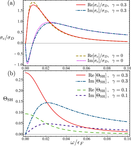
Figure 1: (a) Frequency dependence of the dynamic charge conductivity $\sigma_{c}$, normalized to the Drude conductivity $\sigma_{D}$. (b) Frequency dependence of the dynamic spin Hall angle $\Theta_{\mathrm{SH}}$. Note that for frequencies larger than those corresponding to the Drude peak in the conductivity, the real part of $\Theta_{\mathrm{SH}}$ decays much faster than the imaginary part. In this plot $q=0.01\>k_{F}$ and the elastic collision rate $\tau_{\parallel}=5\>\epsilon_{F}^{-1}$, where $\epsilon_{F}$ ($k_{F}$) is the Fermi energy (momentum). The sign change of the imaginary part of the conductivity for $q\approx 0.01\>k_{F}$ is due to the crossover from the collisionless to the hydrodynamic regime.

We can substitute Eq. (2) into (1) to eliminate the spin current $\bm{J}_{s}$. This gives $\bm{J}_{c}(q,\omega)=\sigma_{c}(q,\omega)\bm{E}(q,\omega)$, where

$$\sigma_{c}(q,\omega)=\frac{\sigma_{m}(q,\omega)}{1+\rho_{ss}\Theta_{\mathrm{SH}}(q,\omega)\sigma_{m}(q,\omega)}$$ (4)

is the dynamic charge conductivity. The dielectric function can be obtained using the continuity equation, $-i\omega\rho_{c}(q,\omega)+i\bm{q}\cdot\bm{J_{c}}(q\omega)=0$, where $\rho_{c}(q,\omega)$ is the charge density. This yields:

$$\epsilon(q,\omega)=1-\frac{\omega_{p}^{2}(q)}{v_{F}^{2}q^{2}}\left(\frac{\chi_{m}(q,\omega)/N(\epsilon_{F})}{1+\rho_{ss}\sigma_{m}(q,\omega)\Theta_{\mathrm{SH}}(q,\omega)}\right),$$ (5)

where $\omega_{p}(q)=\sqrt{4\alpha_{gr}k_{F}v_{F}^{2}q}$ is the plasma frequency of pristine graphene; $\alpha_{gr}=e^{2}/v_{F}$, $N(\epsilon_{F})=2\epsilon_{F}/\pi v_{F}^{2}$ is the density of states at the Fermi energy, and $\chi_{m}(q,\omega)=q^{2}\sigma_{m}(q,\omega)/ie^{2}\omega$ is the Lindhard function including the correction from the particle-number conserving relaxation-time approximation Mermin (1970) (see Sec. III.3). Note that for $\gamma=0$, equations (4) and (5) reduce to the known results for a 2D electron gas with scalar disorder (see e.g. Ref. Giuliani and Vignale, 2005).

A typical plot of $\sigma_{c}(q,\omega)$ as a function of $\omega$, for finite $q$, is shown in Fig. 1(a). The real part of the conductivity exhibits a Drude peak around the plasma frequency and the imaginary part of the conductivity changes sign around the Drude peak. At low frequencies, the system is in the hydrodynamic regime and the imaginary part of the conductivity is negative. However, at high frequencies, the system is in the collisionless regime and the imaginary part of the conductivity is positive. Thus, the sign change in the imaginary part of the conductivity around the Drude peak corresponds to the crossover from the diffusive to collisionless regime. The plot also shows that the corrections to the conductivity due to the extrinsic SHE are small, and most pronounced around the Drude peak frequency.

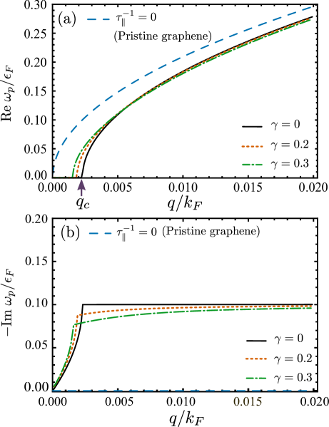
Figure 2: Plasmon dispersion relation (a) and linewidth (b) in doped graphene with SOC disorder leading to an extrinsic SHE, for three different values of $\gamma=\tau_{\parallel}/\tau_{\perp}$, which measures ratio of charge current converted into spin current in the DC limit at zero temperature. The results are plotted for a value of elastic mean free time $\tau_{\parallel}=5\>\epsilon^{-1}_{F}$. As shown in the top panel, increasing $\gamma$ does not have a dramatic effect on the plasmon dispersion and linewidth except near the cutoff wave number $q_{c}$. The black curve is the plasmon dispersion for pristine graphene.

Returning to Eq. (1) and Eq. (2), they can be rearranged as follows:

$$\frac{\bm{J}_{c}(q,\omega)}{\sigma_{m}(q,\omega)}+\rho_{ss}\bm{J}_{s}(q,\omega)\times\bm{\hat{z}}=\bm{E}(q,\omega),$$ (6)

which makes it manifest that the response to AC electric field involves, not only a longitudinal AC charge current, but also a transverse AC spin current, as a result of skew scattering. This is the generalization of the SHE to the AC regime. In particular, notice that the conversion efficiency is determined by the dynamic spin Hall angle $\Theta_{\mathrm{SH}}(q,\omega)$, plotted in Fig. 1(b). It can be seen that the dynamic spin Hall angle diminishes with increasing $\omega$, but remains comparable in magnitude to its DC value around the frequency of the Drude peak. In the DC SHE, the spin current generated by the SHE accumulates at the edge of the sample, and in two dimensional electron gases it has been detected by measurements of Kerr rotation Choi and Cahill (2014) or non-local conductance.Balakrishnan et al. (2014) The AC effect is more challenging to detect, since an oscillating spin current does not produce spin accumulation, but an oscillating magnetization instead. One possible experimental signature, which we discuss below, may be the modification of the plasmon dispersion relation due to the extrinsic SHE.

II.2 Plasmon Frequency and linewidth

We can numerically calculate the plasmon frequency and linewidth from the complex zeros of the dielectric function, Eq. (5). The results are displayed in Fig. 2. The effects of both scalar and SOC disorder on plasmon dispersion are to add a negative imaginary part to $\omega$ (accounting for a damping mechanism), and to “soften” (i.e. red shift) the plasmon frequency at a given wave number $q$ relative to its value in the clean system (cf. Fig. 2).

In the absence of SHE (i.e. $\gamma=0$), our numerical results agree with the formula: Giuliani and Quinn (1984)

$$\omega_{p}(q)=\frac{1+\tilde{q}}{2+\tilde{q}}\left(\sqrt{4\alpha_{gr}\tilde{q}(2+\tilde{q})-\frac{1}{\tau_{\parallel}^{2}}}-\frac{i}{\tau_{\parallel}}\right).$$ (7)

Here $\tilde{q}=q/4\alpha_{gr}k_{F}$ is the dimensionless ratio of the plasmon wave number, $q$, to the the Thomas-Fermi screening wave number, $\alpha_{gr}=e^{2}/v_{F}$ ($v_{F}$ being the Fermi velocity in graphene), and $\tau_{\parallel}$ is the elastic mean free time. Eq. (7) was first obtained by Quinn and Giuliani Giuliani and Quinn (1984) for a 2D electron gas with scalar disorder. More recently, a similar plasmon softening has been found for spin-polarized graphene in Ref. Agarwal et al., 2014.

As shown in Fig. 2, the real part of the plasmon frequency, $\mathrm{Re}\>\omega_{p}\rightarrow 0$ vanishes at a finite (cutoff) wave-number $q_{c}$. Below $q_{c}$, the zero of the dielectric function associated with the plasmon becomes purely imaginary, i.e. the plasmon becomes completely overdamped. For this reason, the cutoff wave number $q_{c}$ is not easily observable since the plasmon becomes a rather ill-defined collective excitation (i.e. $\mathrm{Im}\,\omega_{p}\gg\mathrm{Re}\,\omega_{p}$) before it reaches this wave number.

However, when comparing the $\gamma=0$ and $\gamma\neq 0$ cases, we notice that the overall effects of skew scattering on the plasmon dispersion and lifetime are strongest in the long wave-length limit (cf. Fig. 2). We find that skew scattering causes the softening of the plasmon to occur at smaller wave vector than in the absence of any SOC disorder. It is also interesting to observe in Fig. 2(b) that, as the wave number $q$ increases and consequently the plasmon frequency becomes larger, the shift in the plasmon dispersion relative to the $\gamma=0$ case changes sign for $q\simeq 0.006\>k_{F}$. This happens (roughly) for the value where the plasmon frequency $\omega_{p}(q)\tau_{\parallel}\approx 1$, which corresponds to the crossover from the hydrodynamic to collisionless regime. Skew scattering also modifies the the plasmon linewidth as it can be seen in Fig. 2(b), by decreasing the value of the losses relative to the case with scalar disorder only (i.e. $\gamma=0$).

In order to better discern the effects of SOC disorder from those of scalar disorder, in Fig. 3 we have plotted the relative shift in the plasmon frequency, $\mathrm{Re}\>[\omega_{p}-\omega_{p}(\gamma=0)]/\mathrm{Re}\>\omega_{p}(\gamma=0)$ as a function of $\gamma=\tau_{\parallel}/\tau_{\perp}$. The effect of SOC disorder on the plasmon frequency is more pronounced in the hydrodynamic regime (i.e. for $v_{F}q\tau_{\parallel}\ll 1$ and $\omega\tau_{\parallel}\ll 1$). However, for $\gamma\approx 0.2$, which is comparable to the largest values reported in Ref. Balakrishnan et al., 2014 for CVD graphene, the change in the plasmon frequency at $q=0.01\>k_{F}$ is $\approx 1\>\%$. This small correction may account for the rather similar plasmonic response exhibited CVD and exfoliated graphene. We recall that for the latter, no appreciable SHE has been observed to date (see, e.g. Ref. Balakrishnan et al., 2014). Note as well that the corrections for $q=0.004\>k_{F}$ and $q=0.01\>k_{F}$ have different signs, reflecting the crossover from the hydrodynamic to the collisionless regime taking place for $q\approx 0.006\>k_{F}$, as discussed above.

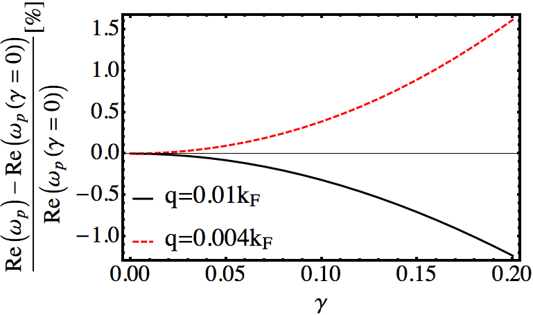
Figure 3: Shift in the plasmon frequency relative to its value for $\gamma=0$ (i.e. in the absence of SOC disorder) for $q=0.1k_{F}$ and $q=0.01k_{F}$. The effect of SOC disorder on the plasmon frequency is more pronounced in the hydrodynamic regime (where $\omega,v_{F}q\ll\tau^{-1}_{\parallel}$). The elastic mean free time is set to $\tau_{\parallel}=5\>\epsilon^{-1}_{F}$.

II.3 Response in long wavelength limit ($q\to 0$)

The plasmon properties discussed in Sec. II.2 are derived for an infinite graphene sheet in a spatially-uniform dielectric environment. However, in practical applications, other geometries, such as semi-infinite plane, discs, et cetera, can be of interest. In such cases, the focus is on the effects of geometry and confinement on the plasmon energy. Such studies rely on solutions of the Maxwell equations whose main input is the conductivity or dielectric function of the material in the long wave-length limit, i.e. for $q\to 0$. Our theory can be incorporated into such numerical schemes, which require the local conductivity as their input.

To leading order in $q\ll k_{F}$, we find (expressions for these functions holding at larger values of $q$ can be found in Appendix D):

$$\sigma_{c}(q,\omega) \simeq\frac{\sigma_{D}}{1-i\omega\tau_{\parallel}}\left[1+\frac{2\gamma^{2}}{(1-i\omega\tau_{\parallel})^{2}}\right],$$ (8)

$$\epsilon(q,\omega)-1 \simeq\frac{-\omega_{p}^{2}(q)}{\omega(\omega+\frac{i}{\tau_{\parallel}})}\left[1+\frac{2\gamma^{2}}{(1-i\omega\tau_{\parallel})^{2}}\right].$$ (9)

In the last expression, $\omega_{p}(q)=\sqrt{4\alpha_{gr}k_{F}v_{F}^{2}q}$ and $\sigma_{D}=\frac{\rho_{0}e^{2}\tau_{\parallel}}{k_{F}/v_{F}}$ are the plasmon frequency and Drude weight, $\rho_{0}$ is the carrier density, and $k_{F}$ ($v_{F}$) is the Fermi momentum (velocity). Note that the corrections to the conductivity and dielectric function due to skew scattering are second order in $\gamma=\tau_{\parallel}/\tau_{\perp}$. This is because the SHE induces a spin current in the transverse direction with magnitude proportional to $\gamma$. However, through the inverse SHE, the spin current produces a charge current in the longitudinal direction, counteracting the original charge current, which introduces another factor of $\gamma$. Thus, even for the large SHE like the one observed in Ref. Balakrishnan et al., 2014 for which $\gamma\sim 0.1$, the correction to the response functions can be small (i.e. few percent). This is also the reason why the effect of SOC disorder on the plasmon properties are rather weak.

Finally, let us point out that, in the long wavelength limit ($q\to 0$), the frequency dependence of the spin Hall angle is given by

$$\Theta_{\mathrm{SH}}(q,\omega)\simeq\frac{\gamma}{1-i\omega\tau_{\parallel}},$$ (10)

which reduces to $\Theta_{\mathrm{SH}}=\gamma$ in the DC limit. It is interesting that the DC spin Hall angle is independent of the order in which the $q\to 0$ and $\omega\to 0$ limits is taken. This is quite different from the behavior exhibited by the conductivity and the dielectric function, whose non-analyticity yields a different result depending on whether $q\to 0$ is taken before or after $\omega\to 0$. The origin of this non-analyticity is the existence of particle-hole excitations in the spectrum of the metal, which is a consequence of the Fermi statistics. On the other hand, the analytical behavior exhibited by the spin Hall angle $\Theta_{\mathrm{SH}}(q,\omega)$ is akin to the behavior of the Hall angle in the Drude theory of the classical Hall effect, which for $q\to 0$ takes a similar form to Eq. (10) with $\gamma$ replaced by $\omega_{c}\tau_{\parallel}$, $\omega_{c}$ being the cyclotron frequency. The analogy implies that the the behavior of the spin Hall angle is unaffected by Fermi statistics, that is, it emerges entirely from skew scattering, which is a single-particle effect.

III Boltzmann transport equation

This section describes the semi-classical Boltzmann Transport Equation (BTE) used to derive the results presented in Sec. II. We consider a graphene sheet decorated with a dilute ensemble of randomly distributed impurities that induce SOC by proximity, such as adatom clusters. Balakrishnan et al. (2014, 2013) In other words, the graphene electrons are subjected to a random SOC potential.

We assume the graphene is electron-doped (hole-doped graphene will exhibit similar physics, due to the particle-hole symmetry of the Hamiltonian of pristine graphene). The transport properties can be calculated using the semi-classical BTE,

$$\partial_{t}n_{\bm{p}\sigma}(\bm{r},t) +\bm{v}_{\bm{p}}\cdot\bm{\nabla}_{\bm{r}}n_{\bm{p}\sigma}(\bm{r},t)$$

$$+e\bm{E}(\bm{r},t)\cdot\bm{\nabla}_{\bm{p}}n_{\bm{p}\sigma}(\bm{r},t)=I[n_{\bm{p}\sigma}(\bm{r},t)],$$ (11)

where $n_{\bm{p}\sigma}(\bm{r},t)$ is the electron distribution function for momentum $\bm{p}$ and spin $\sigma$. The spin quantization axis is perpendicular to the graphene plane, which we take to be the $z$ axis, and $\sigma=\pm 1$ stands for spin pointing in the $\pm\bm{\hat{z}}$ direction. Henceforth, we use the short-hand notation $\bar{\sigma}=-\sigma$, $\bm{v}_{\bm{p}}=v_{F}\bm{\hat{p}}$ ($\bm{\hat{p}}=\bm{p}/|\bm{p}|$) is the group velocity, $v_{F}$ is the Fermi velocity, and $e<0$ is the electron electric charge; $\bm{E}(r,t)$ is the total electric field:

$$\bm{E}(\bm{r},t)=\bm{E}_{ext}(\bm{r},t)-\bm{\nabla}_{\bm{r}}\int d^{2}\bm{r}^{\prime}\frac{\rho(\bm{r}^{\prime},t)}{|\bm{r}-\mathbf{r^{\prime}}|}.$$ (12)

Here, $\bm{E}_{ext}(\bm{r},t)=E_{ext}(\bm{q},\omega)e^{i(\bm{q}\cdot\bm{r}-\omega t)}\,\bm{\hat{x}}$ is the external applied electric field, taken to point in the $\bm{\hat{x}}$ direction, and $\rho(\bm{r},t)=e\sum_{\bm{p},\sigma}n_{\bm{p},\sigma}(\bm{r},t)$ is the charge density.

The BTE applies to the long wavelength limit where $q\ll k_{F}$ and $\omega\ll\epsilon_{F}$, $k_{F}$ ($\epsilon_{F}$) being the Fermi momentum (energy) of doped graphene. The electric field $\bm{E}(\bm{r},t)$ in Eq. (12) must be determined self-consistently, akin to the quantum mechanical treatment of the density-density response function within the random phase approximation (RPA). We have neglected corrections to the BTE arising from the interactions beyond the (time-dependent) Hartree potential since we are interested in the long wave-length properties only, for which the RPA is most accurate.

Next, we assume that the dominant momentum relaxation mechanism arises from scattering with impurities, which is a good approximation at temperatures $T\ll\epsilon_{F}/k_{B}$. In the dilute impurity limit, the collision integral $I[n_{\bm{p}\sigma}]$ takes the following form: Luttinger and Kohn (1958)

$$I[n_{\bm{p}\sigma}]=\sum_{\sigma}\int\frac{d^{2}k}{(2\pi)^{2}}\left(n_{\bm{k}\sigma}-n_{\bm{p}\sigma}\right)W_{\sigma}(\bm{k}\rightarrow\bm{p}),$$ (13)

where

$$W_{\sigma}(\bm{k}\rightarrow\bm{p})=2\pi n_{i}\delta(\epsilon_{p}-\epsilon_{k})\left|T_{\sigma}(\bm{k}\rightarrow\bm{p})\right|^{2}$$ (14)

is the total rate of scattering by the impurities, $n_{i}$ is the mean impurity (areal) density, and $T_{\sigma}(\bm{k}\rightarrow\bm{p})$ is the single-impurity $T$-matrix projected onto the band of the carriers at the Fermi level. For the sake of simplicity and to ascertain the effects of skew-scattering only, in this study we consider SOC disorder that conserves the spin projection along the $z$-axis (which is taken perpendicular to the graphene plane). This requires $[T,s_{z}]=0$, where $s_{z}$ is spin $z$-component. In other words, the proximity-induced SOC disorder must be of the intrinsic (Kane-Mele) type, Ferreira et al. (2014) which is sufficient to explain the data for the DC charge and spin-Hall conductivity from the experiment of Ref. Balakrishnan et al., 2014 (see Appendix A for details).

III.1 Spin-dependent drift velocity ansatz

We solve the BTE by using the following ansatz:

$$n_{\bm{p}\sigma}(\bm{r},t)=\frac{1}{\exp(\beta(\epsilon_{p}-\mu-\bm{v}_{\sigma}(\bm{r},t)\cdot\bm{p}))+1}.$$ (15)

Here, $\beta=1/k_{B}T$ is the inverse absolute temperature ($k_{B}$ is Boltzmann’s constant), $\bm{v}_{\sigma}(\bm{r},t)$ is an undetermined drift velocity which depends on the spin $\sigma$ (we assume that $v_{\sigma}(\bm{r},t)\propto E$); $\mu$ is the global chemical potential of the system, and $\epsilon_{p}=v_{F}p$ is the energy of the graphene electron. To linear order in $\bm{v}_{\sigma}(\bm{r},t)$, the distribution function can be expanded as

$$n_{\bm{p}\sigma}(\bm{r},t) =n^{0}(\epsilon_{p})+\delta n_{\bm{p}\sigma}(\bm{r},t),$$ (16)

$$\delta n_{\bm{p}\sigma}(\bm{r},t) \equiv\left(-\frac{\partial n^{0}(\epsilon_{p})}{\partial\epsilon}\right)\bm{v}_{\sigma}(\bm{r},t)\cdot\bm{p}.$$ (17)

Here, $n^{0}(\epsilon_{p})$ is the equilibrium Fermi-Dirac distribution:

$$n^{0}(\epsilon_{p})=\frac{1}{e^{\beta(\epsilon_{p}-\mu)}+1}.$$ (18)

The charge current $\bm{J}_{c}=eg_{v}\sum_{\bm{p}\sigma}\bm{v}_{p}n_{\bm{p}\sigma}$, and the spin current $\bm{J}_{s}=eg_{v}\sum_{\bm{p}\sigma}\sigma\bm{v}_{p}n_{\bm{p}\sigma}$, are given by

$$\bm{J}_{c}(\bm{r},t) =\frac{e\rho_{0}}{2}\left(\bm{v}_{+}(\bm{r},t)+\bm{v}_{-}(\bm{r},t)\right),$$ (19)

$$\bm{J}_{s}(\bm{r},t) =\frac{e\rho_{0}}{2}\left(\bm{v}_{+}(\bm{r},t)-\bm{v}_{-}(\bm{r},t)\right),$$ (20)

where $\rho_{0}=\sum_{\bm{p}}n^{0}(\epsilon_{p})=g_{v}g_{s}k_{F}^{2}/4\pi$ is the total electron density and $g_{s}=g_{v}=2$ are the spin and valley degeneracies. Note that the spin current is measured in the same units as the charge current, which means that it does not contain the extra factor of $\frac{1}{2}$ (in $\hbar=1$ units) arising from the electron spin angular momentum.

Using the above ansatz and the general form of single-impurity $T$-matrix, the explicit form of the collision integral is obtained (the details are given in Appendix B):

$$I[\delta n_{\bf{p},\sigma}] =-\frac{1}{\tau_{\parallel}(\mu)}\delta n_{\bm{p}\sigma}(\bm{r},t)+\left(\frac{\partial n^{0}}{\partial\bm{p}}\right)\cdot\bm{F}_{\sigma}(\bm{r},t),$$ (21)

$$\bm{F}_{\sigma}(\bm{r},t) \equiv\frac{\epsilon_{F}}{\tau_{\perp}(\mu)v_{F}^{2}}(\bm{v}_{\sigma}(\bm{r},t)\times\bm{\hat{z}})\sigma.$$ (22)

Expressions for the elastic mean free time, $\tau_{\parallel}(\mu)$, and the skew scattering time, $\tau_{\perp}(\mu)$, in terms of the $T$-matrix elements are given in Appendix B. They depend on the chemical potential $\mu$. However, in order to lighten the notation, we will suppress the dependence on $\mu$ in what follows. In Eq. (22), $\bm{F}_{\sigma}(\bm{r},t)$ is an effective Lorentz force which arises from the skew scattering of the SOC disorder-potential. Similar to how the Lorentz force drives a transverse charge current in the Hall effect, this effective “spin-Lorentz force” $\bm{F}_{\sigma}$ drives a transverse spin current. Thus, in the absence of SOC disorder where $\tau^{-1}_{\perp}\rightarrow 0$, $\bm{F}_{\sigma}$ vanishes. The magnitude of the spin-Lorentz force depends on the Fermi energy and $\tau_{\perp}$. For spin up (down) electrons, $\bm{F}_{\sigma}$ points perpendicular to the spin drift velocity of the electron and the positive (negative) spin quantization axis $\bm{\hat{z}}$.

III.2 Particle-number conserving approximation

The conservation of electric charge (i.e. the continuity equation) follows by summing the BTE, Eq. (III), over momentum $\bm{p}$ and spin $\sigma$. L.P. Pitaevskii (1981) This places a constraint on the collision integral: $\sum_{\bm{p},\sigma}I[\delta n_{\bm{p},\sigma}]=0$. However, an ansatz for $\delta n_{\bm{p},\sigma}$ may fail to fulfill the particle-number conservation constraint (see Ref. Kragler and Thomas, 1980 and references therein). Following Mermin’s prescriptionMermin (1970) to satisfy the conservation law, the collision integral must be modified to ensure that the distribution function relaxes to the local (rather than the global, $n^{0}(\epsilon_{p})$) equilibrium distribution function, Kragler and Thomas (1980)

$$g_{p}(\bm{r},t) =\frac{1}{e^{\beta(\epsilon_{p}-\mu-\delta\mu(\bm{r},t))}+1}$$

$$\approx n^{0}(\epsilon_{p})-\frac{\partial n^{0}(\epsilon_{p})}{\partial\epsilon_{p}}\delta\mu(\bm{r},t),$$ (23)

where $\delta\mu(\bm{r},t)$ is the local chemical potential. Thus, the modified collision integral reads

$$\tilde{I}[n_{\bf{p},\sigma}]=-\frac{1}{\tau_{\parallel}}\left[n_{\bm{p}\sigma}(\bm{r},t)-g_{p}(\bm{r},t)\right]\\ +\left(\frac{\partial n^{0}(\epsilon_{p})}{\partial\bm{p}}\right)\cdot\bm{F}_{\sigma}(\bm{r},t).$$ (24)

The local chemical potential, $\delta\mu(\bm{r},t)$, is determined from the constraint $\sum_{p}I[n_{\bm{p}\sigma}]=0$, which yields:

$$\delta\mu(\bm{r},t)=\frac{1}{\sum_{\bm{p}}\frac{\partial n^{0}}{\partial\epsilon}}\sum_{\bm{p}}\delta n_{\bm{p},\sigma}(\bm{r},t).$$ (25)

The modified collision integral, Eq. (24) leads to response functions that interpolate between the collisionless ($\omega\tau_{\parallel}\gg 1$) and the hydrodynamic regimes ($\omega\tau_{\parallel}\ll 1$). Giuliani and Vignale (2005) In this regard, in Appendix C, we show that, as the system enters the hydrodynamic regime, the results of the present particle-number conserving approach to the results of a harmonic mode ansatz, which is appropriate in the hydrodynamic regime.

III.3 Generalized Ohm’s law

We are now ready to solve the linearized BTE and derive the generalized Ohm’s law in the presence of SOC. Recall that the self-consistent electric field has the form

$$\bm{E}(\bm{r},t)=E(\bm{q},\omega)e^{i(\bm{q}\cdot\bm{r}-\omega t)}\,\bm{\hat{x}}.$$ (26)

Without loss of generality, we focus on the relevant Fourier component of $n_{\bm{p}\sigma}(\bm{r},t)=n_{\bm{p}\sigma}(\bm{q},\omega)e^{i(\bm{q}\cdot\bm{r}-\omega t)}$. For notational simplicity, we henceforth suppress the $\bm{q}$ and $\omega$ dependence on $\delta n_{\bm{p},\sigma}$, $v_{\sigma}$, and $E$. Expanding Eq. (III) to linear order in $E$ now gives

$$i(\bm{v}_{\bm{p}}\cdot\bm{q}-\omega)\delta n_{\bm{p}\sigma}+\frac{dn^{0}(\epsilon_{p})}{d\epsilon}\bm{v}_{\bm{p}}\cdot e\bm{E}=\tilde{I}[\delta n_{\bm{p}\sigma}],$$ (27)

with the local particle conserving collision integral Mermin (1970); Kragler and Thomas (1980); Giuliani and Vignale (2005)

$$\tilde{I}[\delta n_{\bf{p},\sigma}]=-\frac{1}{\tau_{\parallel}}\left(\delta n_{\bm{p}\sigma}-\frac{1}{N(\epsilon_{F})}\sum_{p}\delta n_{\bm{p},\sigma}\right)\\ +\left(\frac{\partial n^{0}(\epsilon_{p})}{\partial\bm{p}}\right)\cdot\bm{F}_{\sigma}$$ (28)

Substituting the ansatz (17) into Eq. (27) leads to equations (1) and (2). These equations are the generalized Ohm’s law whose consequences have been discussed in Sec. II. The “skew scattering resistivity” $\rho_{ss}=\frac{k_{F}/v_{F}}{\tau_{\perp}e^{2}v_{F}\rho_{0}}$ has the same form as the Drude resistivity in graphene but with the elastic mean free time $\tau_{\parallel}$ replaced by the skew scattering time $\tau_{\perp}$, and $\rho_{0}=g_{v}k_{F}^{2}/(2\pi)$ is the density of electrons in graphene. Multiplying the skew-scattering resistivity $\rho_{ss}$ by the Drude conductivity yields the spin-dependent electric field, which drives the transverse spin current.

In Eq. (1), $\sigma_{m}(q,\omega)$ represents the local particle conserving charge conductivity, given by

$$\sigma_{m}\left(q,\omega\right) =\frac{\sigma_{0}\left(q,\omega\right)}{M\left(q,\omega\right)},$$ (29)

$$M\left(q,\omega\right) =\frac{1}{N(\mu)}\sum_{\bm{p}}\left(-\frac{\partial n^{0}}{\partial\epsilon}\right)\frac{\omega-\bm{v_{p}}\cdot\bm{q}}{\omega-\bm{v_{p}}\cdot\bm{q}+\frac{i}{\tau_{\parallel}}},$$ (30)

$$\sigma_{0}\left(q,\omega\right) =\frac{4ie^{2}\omega}{q^{2}}\sum_{\bm{p}}\left(-\frac{\partial n^{0}}{\partial\epsilon}\right)\frac{\bm{v_{p}}\cdot\bm{q}}{\omega-\bm{v_{p}}\cdot\bm{q}+\frac{i}{\tau_{\parallel}}}.$$ (31)

Here $M(q,\omega)$ is the dimensionless correction arising from the particle-number conserving collision integral introduced in Sec. III.2. It corrects $\sigma_{0}(q,\omega)$, which does not conserve local particle number, so as to produce a conductivity that is accurate both in hydrodynamic and collisionless regimes. Using the charge continuity equation, we can also define the corrected Lindhard function:

$$\chi_{m}\left(q,\omega\right)=\frac{q^{2}}{ie^{2}\omega}\sigma_{m}\left(q,\omega\right).$$ (32)

Note that $\chi_{m}\left(q,\omega\right)$ corresponds to the semi-classical limit of the Lindhard function in the presence of scalar impurities, and can be derived from Mermin’s result Mermin (1970) (obtained using the quantum Boltzmann equation) in the limit where $q\ll k_{F}$ and $\omega\ll\epsilon_{F}$.

Finally, the spin Hall angle $\Theta_{\mathrm{SH}}$ is defined as the ratio of the spin current to charge current:

$$\Theta_{\mathrm{SH}}(q,\omega)=\left(\frac{i\epsilon_{F}}{\tau_{\perp}\rho_{0}v_{F}^{2}}\right)\sum_{\bm{p}}\left(-\frac{\partial n^{0}}{\partial\epsilon}\right)\frac{\left(\bm{E}/E\cdot(\bm{v}_{p}\times\bm{\hat{z}})\right)^{2}}{\omega-\bm{v_{p}}\cdot\bm{q}+\frac{i}{\tau_{\parallel}}}.$$ (33)

The spin Hall angle stems from the spin Lorentz force introduced in Eq. (22). Thus, we can interpret the charge current in Eq. (1) as being driven by the combination of electric field and a field produced by the spin current.

The expressions for the response functions derived in this section from the solution of the BTE are explicitly evaluated in Appendix D.

IV Summary and Outlook

In this article, we have theoretically investigated the impact of spin-orbit coupling (SOC) disorder on the electrodynamics of two dimensional electron (hole) gases, focusing on doped graphene. This has been achieved by developing a formalism that generalizes previous treatments of the semiclassical transport equations to account for the response of the system to non-uniform time-dependent electric fields. The formalism has allowed us to obtain the explicit forms of the non-local frequency dependent conductivity, dielectric function, and spin Hall angle in the presence of skew scattering. The latter mechanism is responsible for the extrinsic spin Hall effect (SHE), by which a longitudinal charge current is converted into a transverse spin current.

In addition, we have applied our formalism to analyze the effects of SOC disorder on the plasmon dispersion. We have thus found that SOC disorder also decreases the plasmon lifetime and leads to a softening (i.e. red shift relative to the clean system plasma frequency) of the plasmon dispersion. The softening caused by skew scattering is different from the one found for scalar disorder. Giuliani and Quinn (1984) However, as the wave number of the plasmon increases, the corrections to the dispersion arising from skew scattering become smaller to the extent that the it may be hard to discern their effect in a real experiment. This finding suggests that the plasmon softening and linewidth are largely unaffected the SOC disorder that causes the extrinsic SHE. The reason is that, even if a faction $\gamma$ of the longitudinal electric current associated with the plasmon is converted into a transverse spin current by the SHE, the electromagnetic effect of the latter is proportional to $\gamma^{2}$, i.e. the square of the DC spin Hall angle.

It is interesting to discuss the main differences of the electrodynamics developed here with electrodynamics on the surface of 3D topological insulators. Our theory obtains an oscillating transverse spin current is generated when graphene decorated with adatoms is subjected to an AC electric field. This is quite unlike the AC spin currents observed on the surface of 3D topological insulators Di Pietro et al. (2013), which are longitudinal due to the spin-momentum locking taking place at the surface of those materials. In graphenne, this is because the spin current is induced by the SOC disorder via the skew scattering mechanism, which leads to an effective spin-dependent Lorentz force as discussed in Sec. III.

Future extensions of this work (currently underway Huang et al. ) include accounting for spin-flip mechanism by the SOC disorder, and extending the present formalism beyond the semiclassical regime to include, e.g. the effects of inter-band transitions. Concerning the former, preliminary resultsHuang et al. indicate that the picture put forward here is not substantially modified by the presence of other forms of SOC that induce spin-flip scattering.

Finally, we hope that this work will spur the experimental interest to search for SOC-related effects in plasmonics. In the case of graphene, we believe this may be possible through an accurate measurement and comparison of the electrodynamic response of CVD and exfoliated graphene. Unfortunately, the results of our study seem to indicate that from the plasmon properties alone, such effects will be hard to infer. However, other probes may be devised to experimentally detect the alternating spin currents created by the AC SHE. We believe such studies will shed additional light on the mechanisms driving the existence of non-local DC currents.

Appendix A Microscopic model of SOC disorder

In this appendix, we provide the details of the single-impurity $T$-matrix used in the calculation of the collision integral. The form of $T$ is constrained by the symmetries of the total Hamiltonian $H=H_{0}+w(\bm{r})$ where $H_{0}$ is the Hamiltonian of pristine graphene and $w(\bm{r})$ is the (single) impurity potential created by one absorbate (e.g. a cluster of adatoms). In the continuum limit, we model pristine graphene using the $\bm{k}\cdot\bm{p}$ Hamiltonian:

$$H_{0}=v_{F}\left(\tau_{z}\sigma_{x}p_{x}+\sigma_{y}p_{y}\right),$$ (34)

where $v_{F}$ is the Fermi velocity, and $\sigma_{\alpha}$, $\tau_{\alpha}$, $s_{\alpha}$ ($\alpha=x,y,z$) are the Pauli matrices in the Hilbert spaces of the sublattice, valley and electron spins, respectively. Thus, in the continuum limit, the $T$-matrix would be in general a linear combination of 16 matrices $s_{\alpha}\tau_{\beta}$ ($\alpha,\beta=0$ corresponds to the unit matrix).

However, for clusters of adatoms with characteristic size $R\gg a$, where $a=2.46\,$Å  is the interatomic distance in graphene, inter-valley scattering is suppressed. Ferreira et al. (2014); Ochoa et al. (2012) Neglecting inter-valley scattering, the $T$-matrix contains terms proportional to $\tau_{0}$ and $\tau_{z}$. Further assuming that the impurity potential is time-reversal invariant and rotationally invariant, the fully symmetry-constrained form of the the $T$-matrix is obtained: Ferreira et al. (2014)

$$\langle\bm{p}|T|\bm{k}\rangle=a\;s_{0}\tau_{0}+(b\;s_{z}+c\;(\bm{p}-\bm{k})\cdot\bm{s})(\bm{\hat{k}}\wedge\bm{\hat{p}})$$ (35)

where $\hat{\bm{k}}=\bm{k}/k$, $\hat{\bm{p}}=\bm{p}/p$, and $\bm{\hat{k}}\wedge\bm{\hat{p}}=\sin\theta$, $\theta$ being the scattering angle, and $\bm{s}=(s_{x},s_{y})$. Here, $a,b,c$ are functions of $\bm{\hat{k}}\cdot\bm{\hat{p}}=\cos\theta$ which depend on the microscopic details of the scatterer potential. Note that $c$ corresponds to the probability amplitude for spin-flip scattering, which we shall neglect because our study only focuses on the effects of the skew scattering that is described by the term proportional to $b$. This type of models was also a minimal model able to reproduce the experimental data for the DC spin Hall angle and the charge conductivity in Ref. Balakrishnan et al., 2014.

As an example, in order to illustrate a particular form of the $T$-matrix resulting from a concrete microscopic model, let us consider the following Dirac-delta potential:

$$w(\bm{r})=(\lambda_{0}+\lambda_{i}\sigma_{z}\tau_{z}s_{z})\delta(\bm{r}).$$ (36)

The first term in Eq. (36) corresponds to a scalar (spin-independent) potential and the second term corresponds to SOC of the intrinsic (or Kane-Mele Kane and Mele (2005)) type. Notice that both terms in $w(\bm{r})$ potentials commute with $s_{z}$. Thus, within this model, there is no spin flip scattering. Here $\lambda_{0}$ and $\lambda_{i}$ parametrize the scalar and SOC disorder potential strength. Following Ref Yang et al., , the $T$-matrix of this model is computed as,

$$\langle\bm{p}|T|\bm{k}\rangle=\gamma_{0}\cos\left({\frac{\theta}{2}}\right)s_{0}+i\gamma_{i}\sin\left({\frac{\theta}{2}}\right)s_{z}.$$ (37)

$\bm{\hat{k}}\cdot\bm{\hat{p}}=\cos\theta$ is the scattering angle between the incident momentum $\bm{p}$ and scattered electron $\bm{k}$. Note that the spin of the incident and scattered electron is not specified, so the $T$-matrix is a matrix in spin space. The couplings in the above equation are given by:

$$\gamma_{0}=\frac{\lambda_{0}+G_{0}(k)(\lambda_{0}^{2}-\lambda_{i}^{2})}{(G_{0}(k)\lambda_{0}-1)^{2}-(G_{0}(k)\lambda_{I})^{2}},$$ (38)

$$\gamma_{i}=\frac{\lambda_{i}}{(G_{0}(k)\lambda_{0}-1)^{2}-(G_{0}(k)\lambda_{i})^{2}},$$ (39)

where

$$G_{0}(k)=\frac{k}{2\pi v_{F}}\log|kR|-i\frac{k}{4v_{F}},$$ (40)

is the Green function at the origin. Note a short distance cut-off of the order of the inverse of the scatterer radius, $\approx R^{-1}$, has been used to regulate the otherwise divergent integral over $k$. We refer the interested reader to Ref. Yang et al., for details about the derivation of the above results.

Appendix B Collision integral and scattering rates

In this appendix, the elastic mean free time and skew-scattering time are derived from the spin-conserving $T$-matrix (37), by making use of the ansatz introduced in Sec. III. The matrix elements of the $T$-matrix are give by

$$\langle\bm{p}\sigma|T|\bm{k}\sigma^{\prime}\rangle=\left(\gamma_{0}\cos\theta/2+i\gamma_{i}\sigma\sin\theta/2\right)\delta_{\sigma,\sigma^{\prime}}.$$ (41)

By substituting this and Eq. (17) into Eq. (13), we can derive the scattering rates. For example, the spin Lorentz force is derived as follows (recall that $\bm{\hat{k}}\cdot\bm{\hat{p}}=\cos\theta$):

$$I_{2}\equiv 2\pi n_{i}\Big{[}\int \frac{d^{2}k}{(2\pi)^{2}}\text{Im}(\gamma_{0}\gamma_{i})\>\sin\theta\>\delta(\epsilon_{k}-\epsilon_{p})\sigma$$

$$\left(\bm{\hat{k}}-\bm{\hat{p}}\right)\cdot\bm{v}_{\sigma}(\bm{r},t)\left(-\frac{\partial n^{0}}{\partial\epsilon}\right)k_{F}\Big{]}.$$ (42)

Since energy is conserved in collision, we can set $k=|\bm{k}|=|\bm{p}|$ ($\bm{\hat{k}}=\bm{k}/k$, $\bm{\hat{p}}=\bm{p}/k$). Upon expanding $\bm{\hat{k}}=\cos\theta\bm{\hat{p}}+\sin\theta(\bm{\hat{z}}\times\bm{\hat{p}})$, we find that only the term proportional to $\sin\theta$ is non-vanishing upon integration. This leaves

$$I_{2}=2\pi n_{i}\Big{(}\int \frac{d^{2}k}{(2\pi)^{2}}\text{Im(}\gamma_{0}\gamma_{i})\sin^{2}\theta\delta(\epsilon_{k}-\epsilon_{p})\Big{)}$$

$$\sigma\left(\bm{\hat{z}}\times\bm{\hat{p}}\right)\bm{v}_{\sigma}(\bm{r},t)\left(-\frac{\partial n^{0}}{\partial\epsilon}\right)k_{F}.$$ (43)

After some algebra, we arrive at the scattering rate for the (effective) Lorentz spin Hall force:

$$\tau^{-1}_{\perp}=-2\pi n_{i}\int\frac{d^{2}k}{(2\pi)^{2}}\text{Im(}\gamma_{0}\gamma_{i})\sin^{2}\theta\>\delta(\epsilon_{k}-\epsilon_{p}).$$ (44)

As mentioned in Appendix A, the $T$-matrix couplings $\gamma_{0}$ and $\gamma_{i}$ depend on the incoming (electron) energy $\epsilon_{k}=v_{F}k$ and the strength of the scalar and SOC potential $\lambda_{0}$, and $\lambda_{i}$. The sign of the skew scattering rate can be either positive or negative. However, the inverse of the elastic mean free time is always positive and given by

$$\tau^{-1}_{\parallel}=2\pi n_{i}\int\frac{d^{2}k}{(2\pi)^{2}} \left(|\gamma_{0}|^{2}\cos^{2}(\theta/2)+|\gamma_{i}|^{2}\sin^{2}(\theta/2)\right)$$

$$(1-\cos\theta)\delta(\epsilon_{p}-\epsilon_{k}).$$ (45)

Appendix C Comparison between Mermin’s approach and Harmonic Mode Ansatz

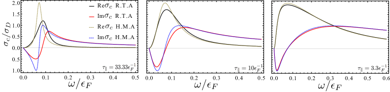
Figure 4: Charge conductivity calculated within the particle-number conserving relaxation time approximation (RTA) and a harmonic mode ansatz (HMA) which is exact in the hydrodynamic regime is plotted against frequency. In order to display the differences as the system is tuned into the hydrodynamic regime, we have fixed $q=0.1\>k_{F}$ and varied the mean free time $\tau_{\parallel}$. In the hydrodynamic limit where $\tau^{-1}_{\parallel}\gg v_{F}q$ and $\tau^{-1}_{\parallel}\gg\omega$ the results of RTA approach very closely the results of HMA. In the opposite limit, i.e. the collisionless limit, the conductivity obtained from the RTA exhibit a broader peak because of the diffusion pole in the conductivity. Giuliani and Vignale (2005)

In this appendix, we compare the response functions obtained using the Boltzmann transport equation (BTE) formulated within Mermin’s particle-number conserving relaxation time approximation (RTA) and a harmonic mode ansatz (HMA) that describes in the hydrodynamic regime where $v_{F}q,\omega\ll\tau^{-1}_{\parallel}$. In the latter regime, equilibration takes place very fast and we can use the following form of the BTE,

$$i(\bm{v}_{\bm{p}}\cdot\bm{q}-\omega)\delta n_{\bm{p}\sigma}+\frac{dn^{0}(\epsilon_{p})}{d\epsilon}\bm{v}_{\bm{p}}\cdot e\bm{E}=I[\delta n_{\bm{p}\sigma}],$$ (46)

where the collision integral, $I[\delta n_{\bm{p}\sigma}]$, is given by Eq. (21). In addition, we can make the following ansatz:

$$\delta n_{\bm{p}\sigma}\approx-\frac{dn_{F}(\epsilon_{p})}{d\epsilon_{p}}\left(C_{\sigma}+A_{\sigma}\cos\theta_{p}+B_{\sigma}\sin\theta_{p}\right).$$ (47)

This is justified since higher angular momentum deformations relax very fast in the hydrodynamic regime. Note that this ansatz is the simplest generalization of the one previously used to account for the DC SHE, Ferreira et al. (2014); Yang et al. which allows for a change in volume of the Fermi surface (a breathing mode). In the above expression, $\cos\theta_{p}=\bm{\hat{p}}\cdot\bm{\hat{x}}$ denotes the cosine of the angle subtended by $\bm{p}$ with the electric field direction, $\bm{\hat{x}}$. The $A_{\sigma}$ and $B_{\sigma}$ terms describe the longitudinal and transverse response, respectively, and $C_{\sigma}$ describes the breathing mode, which is necessary to describe the plasmon mode. In terms of this ansatz, the longitudinal charge conductivity and spin conductivity are given by

$$J_{\parallel}^{c} =eg_{v}\sum_{\bm{p}\sigma}\delta n_{\bm{p}\sigma}\bm{v_{p}}\cdot\bm{\hat{x}}=ev_{F}N(\epsilon_{F})A_{c}/2,$$ (48)

$$J_{\perp}^{s} =eg_{v}\sum_{p\sigma}\sigma\delta n_{p\sigma}\bm{v_{p}}\cdot\bm{\hat{y}}=ev_{f}N(\epsilon_{F})B_{s}/2.$$ (49)

Here, $N(\epsilon_{F})=g_{v}\epsilon_{F}/\pi v_{F}^{2}$ is the density of states at the Fermi energy and $g_{v}=2$ is the valley degeneracy.

Next, we substitute Eq. (47) into Eq. (46). Carrying out the angular average, we derive six equations for the six unknowns $\{A_{\sigma},B_{\sigma},C_{\sigma}\}$, which can be written as:

$$\begin{bmatrix}\omega+\frac{i}{\tau_{\parallel}}&-v_{F}q&\frac{i}{\tau_{\perp}}\\ -v_{F}q&2\omega&0\\ -\frac{i}{\tau_{\perp}}&0&\omega+\frac{i}{\tau_{\parallel}}\end{bmatrix}\begin{bmatrix}A_{s}\\ C_{s}\\ B_{c}\end{bmatrix}=0,$$ (50)

$$\begin{bmatrix}\omega+\frac{i}{\tau_{\parallel}}&-v_{F}q&\frac{i}{\tau_{\perp}}\\ -v_{F}q&2\omega&0\\ -\frac{i}{\tau_{\perp}}&0&\omega+\frac{i}{\tau_{\parallel}}\end{bmatrix}\begin{bmatrix}A_{c}\\ C_{c}\\ B_{s}\end{bmatrix}=\begin{bmatrix}2iev_{F}E\\ 0\\ 0\end{bmatrix}.$$ (51)

Here, we have re-organized the ansatz parameters into spin and charge sectors by defining $A_{s}=A_{\uparrow}-A_{\downarrow}$ and $A_{c}=A_{\uparrow}+A_{\downarrow}$, and similarly definitions for $B_{c},B_{s}$ and $C_{c},C_{s}$. In addition, the scattering rates $\tau^{-1}_{\parallel}=\Gamma_{\sigma}^{S}$ and $\tau^{-1}_{\perp}=\Gamma_{\sigma}^{0}-\Gamma_{\sigma}^{C}$. The three scattering rates $\Gamma_{\sigma}^{0}$, $\Gamma_{\sigma}^{S}$ and $\Gamma_{\sigma}^{C}$ are defined as follows:

$$\frac{\Gamma_{\sigma}^{S}}{N(\mu)} =\int\frac{d\theta_{p}d\theta_{k}}{(2\pi)^{2}}W_{\sigma}(\bm{k}\rightarrow\bm{p})\sin(\theta_{p}-\theta_{k}),$$ (52)

$$\frac{\Gamma_{\sigma}^{C}}{N(\mu)} =\int\frac{d\theta_{p}d\theta_{k}}{(2\pi)^{2}}W_{\sigma}(\bm{k}\rightarrow\bm{p})\cos(\theta_{p}-\theta_{k}),$$ (53)

$$\frac{\Gamma_{\sigma}^{0}}{N(\mu)} =\int\frac{d\theta_{p}d\theta_{k}}{(2\pi)^{2}}W_{\sigma}(\bm{k}\rightarrow\bm{p}).$$ (54)

The scattering rate $W_{\sigma}(\bm{k}\rightarrow\bm{p})$ is defined in Eq. (14). The ratio $\gamma=\tau_{\parallel}/\tau_{\perp}$ is the (zero temperature) spin Hall angle Ferreira et al. (2014), which measures the relative magnitude of transverse spin current over longitudinal charge current. Eq. (50) states that the applied AC electric field does not couple to the longitudinal spin response ($A_{s}$), the net spin response ($C_{s}$), or the transverse charge response ($B_{c}$), as might be expected on physical grounds. We hence ignore these three quantities. The terms which do couple to the electric field, collected in Eq. (51), are the longitudinal charge response ($A_{c}$) and net charge response ($C_{c}$), as well as the transverse spin response ($B_{s}$). The solution is

$$A_{c} =\frac{2iev_{F}E}{\omega+i/\tau_{\parallel}-\frac{1}{\tau_{\perp}^{2}}\frac{1}{\omega+i/\tau_{\parallel}}-\frac{(v_{F}q)^{2}}{2\omega}}$$ (55)

$$B_{s} =\frac{i/\tau_{\perp}}{\omega+i/\tau_{\parallel}}\,A_{c}$$ (56)

$$C_{c} =\frac{v_{F}q}{2\omega}\,A_{c}.$$ (57)

Substituting these solutions into Eq. (48) and Eq. (49) gives us the charge and spin response in the hydrodynamic limit. Thus, as an example, in Fig. 4 we show that the agreement of charge conductivity computed within Mermin’s RTA and the hydrodynamic ansatz employed in this appendix agrees as the hydrodynamic regime (where $\tau^{-1}_{\parallel}\gg\omega$ and $\tau^{-1}_{\parallel}\gg v_{F}q$) is approached. On the other hand, in the collisionless regime, the results from the harmonic-mode ansatz are inaccurate since the ansatz of Eq. 47 neglects large angular momentum deformations of the Fermi surface.

Appendix D Evaluation of response functions

In this appendix, the explicit formula of the dielectric function (cf. Eq. 5) and charge conductivity (cf. Eq. 4) are provided. The expressions are most simply written in terms of the dimensionless ratios $\nu=\omega/(v_{F}q)$ and $\eta=1/(\tau_{\parallel}v_{F}q)$. In what follows, we shall use the following formula (see e.g. Ref. Giuliani and Vignale, 2005 for details):

$$I_{1}=\int\frac{d\theta}{2\pi}\frac{1}{\nu+i\eta-\cos\theta}=\frac{1}{\sqrt{(\nu+i\eta)^{2}-1}},$$ (58)

Hence, the standard Lindhard function (normalized to density of states at the Fermi energy) can be evaluted as follows:

$$\frac{\chi_{0}(q,\omega)}{N(\epsilon_{F})}= \frac{1}{N(\epsilon_{F})}\sum_{\bm{p}}\left(-\frac{\partial n^{0}}{\partial\epsilon}\right)\frac{\bm{v_{p}}\cdot\bm{q}}{\omega-\bm{v_{p}}\cdot\bm{q}+\frac{i}{\tau_{\parallel}}}$$

$$= \int^{2\pi}_{0}\frac{d\theta}{2\pi}\frac{v_{F}q\cos\theta}{\omega+\frac{i}{\tau_{\parallel}}-v_{F}q\cos\theta}$$

$$= (\nu+i\eta)I_{1}-1.$$ (59)

Likewise, the ”Mermin factor” (cf. Eq. 30) that modified the Lindhard function in order to conserve the particle number is similarly evaluated as follows:

$$M\left(q,\omega\right) =\frac{1}{N(\mu)}\sum_{\bm{p}}\left(-\frac{\partial n^{0}}{\partial\epsilon}\right)\frac{\omega-\bm{v_{p}}\cdot\bm{q}}{\omega-\bm{v_{p}}\cdot\bm{q}+\frac{i}{\tau_{\parallel}}}$$

$$=1-i\eta\>I_{1}.$$ (60)

Collecting these results, we obtain the Lindhard function within Mermin’s particle-number conserving approximation,

$$\frac{\chi_{m}(q,\omega)}{N(\epsilon_{F})} =\frac{(\nu+i\eta)I_{1}-1}{1-i\eta I_{1}}$$ (61)

$$=\left(\frac{\nu}{\sqrt{(\nu+i\eta)^{2}-1}-i\eta}-1\right).$$ (62)

From this expresion, the conductivity can be easily obtained using Eq. (32). Similarly, the dynamic spin Hall angle $\Theta_{\mathrm{SH}}(q,\omega)$ defined in Eq.(33) is evaluated as follow

$$\Theta_{\mathrm{SH}}(q,\omega)= \frac{2i}{v_{F}\tau_{\perp}q}\int^{2\pi}_{0}\frac{d\theta}{2\pi}\frac{\sin^{2}\theta}{\nu+i\gamma-\cos\theta}$$

$$= \frac{2i}{v_{F}\tau_{\perp}q}\Bigg{[}\frac{2}{z_{+}-z_{-}}$$

$$+\frac{1}{2}\left(\frac{z_{-}^{4}+2z_{-}^{2}+1}{z_{-}^{2}(z_{-}-z_{+})}+\frac{1}{z_{-}}+\frac{1}{z_{+}}\right)\Bigg{]},$$ (63)

where $z_{\pm}=\nu+i\eta\pm\sqrt{(\nu+i\eta)^{2}-1}$. Using the explicit form of $\Theta_{\mathrm{SH}}(q,\omega)$ and $\sigma_{m}(q,\omega)$ the charge conductivity in Eq.(4) and the dielectric function in Eq.(5) can be obtained. Since they are lengthier than the above expressions and not particularly illuminating, we shall not reproduce them here explicitly.

References

- Stauber (2014) T. Stauber, Journal of Physics: Condensed Matter 26, 123201 (2014).
- Ju et al. (2011) L. Ju, B. Geng, J. Horng, C. Girit, M. Martin, Z. Hao, H. A. Bechtel, X. Liang, A. Zettl, Y. R. Shen, et al., Nature nanotechnology 6, 630 (2011).
- Di Pietro et al. (2013) P. Di Pietro, M. Ortolani, O. Limaj, A. Di Gaspare, V. Giliberti, F. Giorgianni, M. Brahlek, N. Bansal, N. Koirala, S. Oh, et al., Nature nanotechnology 8, 556 (2013).
- Grigorenko et al. (2012) A. Grigorenko, M. Polini, and K. Novoselov, Nature photonics 6, 749 (2012).
- Chen et al. (2012) J. Chen, M. Badioli, P. Alonso-González, S. Thongrattanasiri, F. Huth, J. Osmond, M. Spasenović, A. Centeno, A. Pesquera, P. Godignon, et al., Nature 487, 77 (2012).
- Huertas-Hernando et al. (2006) D. Huertas-Hernando, F. Guinea, and A. Brataas, Physical Review B 74, 155426 (2006).
- Min et al. (2006) H. Min, J. Hill, N. A. Sinitsyn, B. Sahu, L. Kleinman, and A. H. MacDonald, Physical Review B 74, 165310 (2006).
- Balakrishnan et al. (2013) J. Balakrishnan, G. K. W. Koon, M. Jaiswal, A. C. Neto, and B. Özyilmaz, Nature Physics 9, 284 (2013).
- Balakrishnan et al. (2014) J. Balakrishnan, G. K. W. Koon, A. Avsar, Y. Ho, J. H. Lee, M. Jaiswal, Baeck, et al., Nature communications 5, 4748 (2014).
- Weeks et al. (2011) C. Weeks, J. Hu, J. Alicea, M. Franz, and R. Wu, Phys. Rev. X 1, 021001 (2011).
- (11) L. Brey, arXiv:1509.04024 .
- Jiang et al. (2012) H. Jiang, Z. Qiao, H. Liu, J. Shi, and Q. Niu, Phys. Rev. Lett. 109, 116803 (2012).
- Wang et al. (2015) Y. Wang, X. Cai, J. Reutt-Robey, and M. S. Fuhrer, Phys. Rev. B 92, 161411 (2015).
- Kaverzin and van Wees (2015) A. A. Kaverzin and B. J. van Wees, Phys. Rev. B 91, 165412 (2015).
- Sinova et al. (2015) J. Sinova, S. O. Valenzuela, J. Wunderlich, C. H. Back, and T. Jungwirth, Rev. Mod. Phys. 87, 1213 (2015).
- Dyakonov and Perel (1971) M. Dyakonov and V. Perel, Physics Letters A 35, 459 (1971).
- Hirsch (1999) J. Hirsch, Phys. Rev. Lett 83, 1834 (1999).
- Zhang (2000) S. Zhang, Phys. Rev. Lett. 85, 393 (2000).
- Vignale (2010) G. Vignale, Journal of superconductivity and novel magnetism 23, 3 (2010).
- Schliemann (2006) J. Schliemann, International Journal of Modern Physics B 20, 1015 (2006).
- Castro Neto and Guinea (2009) A. H. Castro Neto and F. Guinea, Phys. Rev. Lett. 103, 026804 (2009).
- Ferreira et al. (2014) A. Ferreira, T. G. Rappoport, M. A. Cazalilla, and A. H. Castro Neto, Phys. Rev. Lett. 112 (2014).
- Kato et al. (2004) Y. Kato, R. Myers, A. Gossard, and D. Awschalom, Science 306, 1910 (2004).
- Wunderlich et al. (2005) J. Wunderlich, B. Kaestner, J. Sinova, and T. Jungwirth, Physical review letters 94, 047204 (2005).
- Seki et al. (2008) T. Seki, Y. Hasegawa, S. Mitani, S. Takahashi, H. Imamura, S. Maekawa, J. Nitta, and K. Takanashi, Nature Materials 7, 125 (2008).
- Liu et al. (2011) L. Liu, T. Moriyama, D. Ralph, and R. Buhrman, Phys. Rev. Lett 106, 036601 (2011).
- Liu et al. (2012) L. Liu, C.-F. Pai, Y. Li, H. Tseng, D. Ralph, and R. Buhrman, Science 336, 555 (2012).
- Nagaosa et al. (2010) N. Nagaosa, J. Sinova, S. Onoda, A. H. MacDonald, and N. P. Ong, Rev. Mod. Phys. 82, 1539 (2010).
- Gmitra et al. (2013) M. Gmitra, D. Kochan, and J. Fabian, Phys. Rev. Lett. 110, 246602 (2013).
- Irmer et al. (2015) S. Irmer, T. Frank, S. Putz, M. Gmitra, D. Kochan, and J. Fabian, Phys. Rev. B 91, 115141 (2015).
- Sinova and MacDonald (2008) J. Sinova and A. H. MacDonald, Theory of Spin-Orbit Effects in Semiconductors (Academic Press, 2008).
- Principi et al. (2013) A. Principi, G. Vignale, M. Carrega, and M. Polini, Phys. Rev. B 88, 121405 (2013).
- (33) H. Yang, C. Huang, H. Ochoa, and M. A. Cazalilla, arXiv:1510.07771v1 .
- Uchida et al. (2015) K. Uchida, H. Adachi, D. Kikuchi, S. Ito, Z. Qiu, S. Maekawa, and E. Saitoh, Nature communications 6 (2015).
- Mermin (1970) N. D. Mermin, Phys. Rev. B 1, 2362 (1970).
- Giuliani and Quinn (1984) G. F. Giuliani and J. J. Quinn, Phys. Rev. B 29, 2321 (1984).
- Agarwal et al. (2014) A. Agarwal, M. Polini, G. Vignale, and M. E. Flatté, Phys. Rev. B 90, 155409 (2014).
- Fei et al. (2012) Z. Fei, A. Rodin, G. Andreev, W. Bao, A. McLeod, M. Wagner, L. Zhang, Z. Zhao, M. Thiemens, G. Dominguez, et al., Nature 487, 82 (2012).
- Giuliani and Vignale (2005) G. Giuliani and G. Vignale, Quantum Theory of the Electron Liquid (Cambridge University Press, 2005).
- Choi and Cahill (2014) G.-M. Choi and D. G. Cahill, Phys. Rev. B 90, 214432 (2014).
- Luttinger and Kohn (1958) J. M. Luttinger and W. Kohn, Phys. Rev. 109, 1892 (1958).
- L.P. Pitaevskii (1981) E. L.P. Pitaevskii, Physical Kinetics: Volume 10 (Course of Theoretical Physics) (Pergamon Press plc, 1981).
- Kragler and Thomas (1980) R. Kragler and H. Thomas, Zeitschrift für Physik B Condensed Matter 39, 99 (1980).
- (44) C. Huang, Y. Chong, G. Vignale, and M. A. Cazalilla, In preparation.
- Ochoa et al. (2012) H. Ochoa, A. H. Castro Neto, V. I. Fal’ko, and F. Guinea, Phys. Rev. B 86, 245411 (2012).
- Kane and Mele (2005) C. L. Kane and E. J. Mele, Phys. Rev. Lett 95, 226801 (2005).