Information Flows?
A Critique of Transfer Entropies

Information Flows?
A Critique of Transfer Entropies

Abstract

A central task in analyzing complex dynamics is to determine the loci of information storage and the communication topology of information flows within a system. Over the last decade and a half, diagnostics for the latter have come to be dominated by the transfer entropy. Via straightforward examples, we show that it and a derivative quantity, the causation entropy, do not, in fact, quantify the flow of information. At one and the same time they can overestimate flow or underestimate influence. We isolate why this is the case and propose several avenues to alternate measures for information flow. We also address an auxiliary consequence: The proliferation of networks as a now-common theoretical model for large-scale systems, in concert with the use of transfer-like entropies, has shoehorned dyadic relationships into our structural interpretation of the organization and behavior of complex systems. This interpretation thus fails to include the effects of polyadic dependencies. The net result is that much of the sophisticated organization of complex systems may go undetected.

Keywords: stochastic process, transfer entropy, causation entropy, partial information decomposition, network science

An important task in understanding a complex system is determining its information dynamics and information architecture—what mechanisms generate information, where is that information stored, and how is it transmitted within a system? While this pursuit goes back perhaps as far as Shannon’s foundational work on communication [1], in many ways it was Kolmogorov [2, 3, 4] who highlighted the transmission of information from the micro- to the macroscales as central to the behavior of complex systems. Later, Lin showed that “information flow” is key to understanding network controllability [5] and Shaw speculated that such flows between information sources and sinks is a necessary descriptive framework for spatially extended chaotic systems—an alternative to narratives based on tracking energy flows [6, Sec. 14].

A common thread in these works is quantifying the flow of information. To facilitate our discussion, let’s first consider an intuitive definition: Information flow from process $X$ to process $Y$ is the existence of information that is currently in $Y$, the “cause” of which can be solely attributed to $X$’s past. If information can be solely attributed in such a manner, we refer to it as localized. This notion of localized flow mirrors the intuitive general definitions of “causal” flow proposed by Granger [7] and, before that, Wiener [8].

Ostensibly to measure information flow—and notably much later than the above efforts—Schreiber introduced the transfer entropy [9] as the information shared between $X$’s past and the present $Y_{t}$, conditioning on information from $Y$’s past. Perhaps not surprisingly, given the broad and pressing need to probe the organization of modern life’s increasingly complex systems, the transfer entropy’s use has been substantial—over the last decade and a half, its introduction alone garnered an average of $100$ citations per year.

The primary goal of the following is to show that the transfer entropy does not, in fact, measure information flow, specifically in that it attributes an information source to influences that are not localizable and so not flows. We draw out the interpretational errors, some quite subtle, that result—including overestimating flow, underestimating influence, and more generally misidentifying structure when modeling complex systems as networks with edges given by transfer entropies.

Identifying shortcomings in the transfer entropy is not new. Smirnov [10] pointed out three: Two relate to how it responds to using undersampled empirical distributions and are therefore not conceptual issues with the measure. The third, however, was its inability to differentiate indirect influences from direct influences. This weakness motivated Sun and Bollt to propose the causation entropy [11]. While their measure does allow differentiating between direct and indirect effects via the addition of a third hidden variable, it too ascribes an information source to unlocalizable influences.

Our exposition reviews the notation and information theory needed and then considers two rather similar examples—one involving influences between two processes and the other, influences among three. They make operational what we mean by “localized”, “flow”, and “influence”, leading to the conclusion that the transfer entropy fails to capture information flow. We close by discussing a distinctive philosophy underlying our critique and then turn to possible resolutions and to concerns about modeling practice in network science.

Background

Following standard notation [12], we denote random variables with capital letters and their associated outcomes using lower case. For example, the observation of a coin flip might be denoted $X$, while the coin actually landing Heads or Tails would be $x$. Emphasizing temporal processes, we subscript a random variable with a time index; e.g., the random variable representing a coin flip at time $t$ is denoted $X_{t}$. We denote a temporally contiguous block of random variables (a time series) using a Python-slice-like notation $X_{i:j}=X_{i}X_{i+1}\ldots X_{j-1}$, where the final index is exclusive. When $X_{t}$ is distributed according to $\Pr(X_{t})$, we denote this as $X_{t}\sim\Pr(X_{t})$. We assume familiarity with basic information measures, specifically the Shannon entropy $\operatorname{H}\left[X\right]$, mutual information $\operatorname{I}\left[X:Y\right]$, and their conditional forms $\operatorname{H}\left[X~{}\middle|~{}Z\right]$ and $\operatorname{I}\left[X:Y~{}\middle|~{}Z\right]$ [12].

The transfer entropy $\operatorname{T}_{X\rightarrow Y}$ from time series $X$ to time series $Y$ is the information shared between $X$’s past and $Y$’s present, given knowledge of $Y$’s past [9]:

$$\operatorname{T}_{X\rightarrow Y} =\operatorname{I}\left[Y_{t}:X_{0:t}~{}\middle|~{}Y_{0:t}\right]~{}.$$ (1)

Intuitively, this quantifies how much better one predicts $Y_{t}$ using both $X_{0:t}$ and $Y_{0:t}$ over using $Y_{0:t}$ alone. A nonzero value of the transfer entropy certainly implies a kind of influence of $X$ on $Y$. Our questions are: Is this influence necessarily via information flow? Is it necessarily direct?

Addressing the last question, the causation entropy $\operatorname{\mathcal{C}}_{X\rightarrow Y|\left(Y,Z\right)}$ is similar to the transfer entropy, but conditions on the past of a third (or more) time series [11]:

$$\operatorname{\mathcal{C}}_{X\rightarrow Y|\left(Y,Z\right)} =\operatorname{I}\left[Y_{t}:X_{0:t}~{}\middle|~{}Y_{0:t},Z_{0:t}\right]~{}.$$ (2)

(It is also known as the conditional transfer entropy.) The primary improvement over $\operatorname{T}_{X\rightarrow Y}$ is the causation entropy’s ability to determine if a dependency is indirect (i.e., mediated by the third process $Z$) or not. Consider, for example, the following system $X\to Z\to Y$: variable $X$ influences $Z$ and $Z$ in turn influences $Y$. Here, any influence that $X$ has on $Y$ must pass through $Z$. In this case, the transfer entropy $\operatorname{T}_{X\rightarrow Y}>$0\text{\,}\mathrm{bit}$$ even though $X$ does not directly influence $Y$. The causation entropy $\operatorname{\mathcal{C}}_{X\rightarrow Y|\left(Y,Z\right)}=$0\text{\,}\mathrm{bit}$$, however, due to conditioning on $Z$.

Many concerns and pitfalls in applying information measures comes not in their definition, estimation, or derivation of associated properties. Rather, many arise in interpreting results. Properly interpreting the meaning of a measure can be the most subtle and important task we face when using measures to analyze a system’s structure, as we will now demonstrate. Furthermore, while these examples may seem pathological, they were chosen for their transparency and simplicity; similar failures arise in Gaussian systems [13] signifying that the issue at hand is widespread.

Example: Two Time Series

Consider two time series, say $X$ and $Y$, given by the probability laws:

$$X_{t} \thicksim\begin{cases}0&\textrm{with probability }\nicefrac{{1}}{{2}}\\ 1&\textrm{with probability }\nicefrac{{1}}{{2}}\end{cases}~{},$$

$$Y_{0} \thicksim\begin{cases}0&\textrm{with probability }\nicefrac{{1}}{{2}}\\ 1&\textrm{with probability }\nicefrac{{1}}{{2}}\end{cases}~{},~{}\text{and}$$

$$Y_{t} =X_{t-1}\oplus Y_{t-1}~{};$$

that is, $X_{t}$ and $Y_{0}$ are independent and take values 0 and 1 with equal probability, and $y_{t}$ is the Exclusive OR of the prior values $x_{t-1}$ and $y_{t-1}$. By a straightforward calculation we find that $\operatorname{T}_{X\rightarrow Y}=$1\text{\,}\mathrm{bit}$$. Does this mean that one bit of information is being transferred from $X$ to $Y$ at each time step? Let’s take a closer look.

We first observe that the amount of information in $Y_{t}$ is $\operatorname{H}\left[Y_{t}\right]=$1\text{\,}\mathrm{bit}$$. Therefore, the uncertainty in $Y_{t}$ can be reduced by at most $1\text{\,}\mathrm{bit}$. Furthermore, the information shared by $Y_{t}$ and the prior behavior of the two time series is $\operatorname{I}\left[Y_{t}:\left(X_{0:t},Y_{0:t}\right)\right]=$1\text{\,}\mathrm{bit}$$. And so, the $1\text{\,}\mathrm{bit}$ of $Y_{t}$’s uncertainty in fact can be removed by the prior observations of both time series.

How much does $Y_{0:t}$ alone help us predict $Y_{t}$? We quantify this using mutual information. Since $\operatorname{I}\left[Y_{t}:Y_{0:t}\right]=$0\text{\,}\mathrm{bit}$$, the variables are independent: $Y_{0:t}$ alone does not help in predicting $Y_{t}$. However, knowing $Y_{0:t}$, how much does $X_{0:t}$ help in predicting $Y_{t}$? The conditional mutual information $\operatorname{I}\left[Y_{t}:X_{0:t}~{}\middle|~{}Y_{0:t}\right]=$1\text{\,}\mathrm{bit}$$—the transfer entropy we just computed—quantifies this. This situation is graphically analyzed via the information diagram (I-diagram) [14] in Fig. 1a.

To obtain a more complete picture of the information dynamics under consideration, let’s reverse the order in which the time series are queried. The mutual information $\operatorname{I}\left[Y_{t}:X_{0:t}\right]=$0\text{\,}\mathrm{bit}$$ tells us that the $X$ time series alone does not help predict $Y_{t}$. However, the conditional mutual information $\operatorname{I}\left[Y_{t}:Y_{0:t}~{}\middle|~{}X_{0:t}\right]=$1\text{\,}\mathrm{bit}$$. And so, from this point of view it is $Y$’s past that helps predict $Y_{t}$, contradicting the preceding analysis. This complementary situation is presented diagrammatically in Fig. 1b.

How can we rectify the seemingly inconsistent conclusions drawn by these two lines of reasoning? The answer is quite straightforward: the $1\text{\,}\mathrm{bit}$ of information about $Y_{t}$ does not come from either time series individually, but rather from both of them simultaneously. (In fact, the I-Diagrams are naturally consistent, once one recognizes that the co-information [15], the inner-most information atom, is $\operatorname{I}\left[Y_{t}:X_{0:t}:Y_{0:t}\right]=$-1\text{\,}\mathrm{bit}$$.)

In short, the $1\text{\,}\mathrm{bit}$ of reduction in uncertainty $\operatorname{H}\left[Y_{t}\right]$ should not be localized to either time series. The transfer entropy, however, erroneously localizes this information to $X_{0:t}$. In light of this, the transfer entropy overestimates information flow.

This example shows that the transfer entropy can be positive due not to information flow, but rather to nonlocalizable influence—in this case, a conditional dependence between variables. This suggests that, though inappropriate for measuring information flow, the transfer entropy may be a viable measure of such influence. Our next example illustrates that this too is incorrect.

(a) $Y_{0:t}$ alone does not predict $Y_{t}$. (The -shaped region $\operatorname{I}\left[Y_{0:t}:Y_{t}\right]=$0\text{\,}\mathrm{bit}$$.) However, when used in conjunction with $X_{0:t}$, they completely predict its value. (The -shaped region $\operatorname{I}\left[X_{0:t}:Y_{t}~{}\middle|~{}Y_{0:t}\right]=$1\text{\,}\mathrm{bit}$$.)

(b) $X$’s past $X_{0:t}$ alone does not aid in predicting $Y_{t}$. (The -shaped region $\operatorname{I}\left[X_{0:t}:Y_{t}\right]=$0\text{\,}\mathrm{bit}$$.) However, given knowledge of $X_{0:t}$, then $Y_{0:t}$ can predict $Y_{t}$. (The -shaped region $\operatorname{I}\left[Y_{0:t}:Y_{t}~{}\middle|~{}X_{0:t}\right]=$1\text{\,}\mathrm{bit}$$.)

Figure 1: Two complementary ways to view the information shared between $X_{0:t},Y_{0:t}$, and $Y_{t}$. In each I-Diagram, a circle represents a random variable whose area measures the random variable’s entropy. Overlapping regions are information that is shared. The transfer entropy is a conditional mutual information; a region where two random variables overlap, but that falls outside the random variable being conditioned on.

Example: Three Time Series

Our second example parallels the first. Before, we considered the case where one of two time series is determined by the past of both, we now consider the case where two time series determine a third, again via an Exclusive OR operation. Their probability laws are:

$$X_{t} \thicksim\begin{cases}0&\textrm{with probability }\nicefrac{{1}}{{2}}\\ 1&\textrm{with probability }\nicefrac{{1}}{{2}}\end{cases}~{},$$

$$Y_{t} \thicksim\begin{cases}0&\textrm{with probability }\nicefrac{{1}}{{2}}\\ 1&\textrm{with probability }\nicefrac{{1}}{{2}}\end{cases}~{},~{}\text{and}$$

$$Z_{t} =X_{t-1}\oplus Y_{t-1}~{},$$

in which $z_{0}$’s value is irrelevant. Unlike the prior example, the transfer entropy from either $X$ or $Y$ to $Z$ is zero: $\operatorname{T}_{X\rightarrow Z}=\operatorname{T}_{Y\rightarrow Z}=$0\text{\,}\mathrm{bit}$$, and it therefore underestimates influence that is present. Furthermore, the relevant pairwise mutual informations all vanish: $\operatorname{I}\left[Z_{t}:X_{0:t}\right]=\operatorname{I}\left[Z_{t}:Y_{0:t}\right]=\operatorname{I}\left[Z_{t}:Z_{0:t}\right]=$0\text{\,}\mathrm{bit}$$. The time series are pairwise independent.

Given that we are probing the influences between three time series, it is natural now to consider the behavior of the causation entropy. In this case, we have $\operatorname{\mathcal{C}}_{X\rightarrow Z|\left(Y,Z\right)}=\operatorname{\mathcal{C}}_{Y\rightarrow Z|\left(X,Z\right)}=$1\text{\,}\mathrm{bit}$$, indicating that given the past behavior of $Z$ and $X$ (or $Y$), the past of $Y$ (or $X$) can be used to predict the behavior of $Z_{t}$. Like before, this $1\text{\,}\mathrm{bit}$ of information cannot be localized to either $X$ or $Y$ and so it is inaccurate to ascribe the $1\text{\,}\mathrm{bit}$ of information in $Z_{t}$ to either $X$ or $Y$ alone. In this way, the causation entropy also erroneously localizes the $1\text{\,}\mathrm{bit}$ of joint influence. While the causation entropy succeeds here as a measure of nonlocalizable influence, as a measure of information flow, it overestimates. (This is known to Sun and Bollt, but here we stress that the failure is a general issue with interpreting its value, not merely a limitation regarding network inference.) These information quantities are displayed in the I-Diagram in Fig. 2.

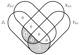
Figure 2: Information diagram depicting both transfer entropies and causation entropies for three times series $X$, $Y$, and $Z$. $\operatorname{T}_{X\rightarrow Z}=$0\text{\,}\mathrm{bit}$$ corresponds to the two regions shaded with south-east sloping lines and $\operatorname{T}_{Y\rightarrow Z}=$0\text{\,}\mathrm{bit}$$, the two regions shaded with north-east sloping lines. $\operatorname{\mathcal{C}}_{X\rightarrow Z|\left(Y,Z\right)}=$1\text{\,}\mathrm{bit}$$ is the region containing only south-east sloping lines and, similarly, $\operatorname{\mathcal{C}}_{Y\rightarrow Z|\left(X,Z\right)}=$1\text{\,}\mathrm{bit}$$ is the region containing only north-east sloping lines.

Discussion

We see that transfer-like entropies can both overestimate information flow (first example) and underestimate influence (second example). The primary misunderstanding of these quantities stems from a mischaracterization of the conditional mutual information. Most basically, probabilistic conditioning is not a “subtractive” operation: $\operatorname{I}\left[X:Y~{}\middle|~{}Z\right]$ is not the information shared by $X$ and $Y$ once the influences of $Z$ have been removed. Rather, it is the information shared by $X$ and $Y$ taking into account $Z$. This is not a game of mere semantics: Conditioning can increase the information shared between two processes: $\operatorname{I}\left[X:Y\right]<\operatorname{I}\left[X:Y~{}\middle|~{}Z\right]$. This cannot happen if conditioning merely removed influence: conditional dependence includes additional dependence that occurs in the presence of a third variable [16]. Measuring information flow—as we have defined it—requires a method of localizing information. Since simple conditioning can fail to localize information, the transfer entropy, causation entropy, and other measures utilizing the conditional mutual information can fail as measures of information flow.

Another way to understand conditional dependence is through the partial information decomposition [17]. Within this framework, the mutual information between two random variables $X_{1}$ and $X_{2}$ (call them inputs) and a third random variable $Y$ (the output) is decomposed into four mutually exclusive components: $\operatorname{I}\left[(X_{1},X_{2}):Y\right]=R+U_{1}+U_{2}+S$. $R$ quantifies how the inputs $X_{1}$ and $X_{2}$ redundantly inform the output $Y$, $U_{1}$ and $U_{2}$ quantify how each provides unique information to $Y$, and finally $S$ quantifies how the inputs together synergistically inform the output. In this decomposition, the mutual information between one input and the output is equal to what uniquely comes from that input plus what is redundantly provided by both inputs; $\operatorname{I}\left[X_{1}:Y\right]=R+U_{1}$, for example. However, the mutual information between that input and the output conditioned on the other input is equal to what uniquely comes from that one input, plus what is synergistically provided by both inputs: $\operatorname{I}\left[X_{1}:Y~{}\middle|~{}X_{2}\right]=U_{1}+S$. In other words, conditioning removes the redundant information, but adds the synergistic information. Here, conditional dependencies manifest themselves as synergy.

Treating $X_{0:t}$ and $Y_{0:t}$ as inputs and $Y_{t}$ as output, the partial information decomposition identifies the transfer entropy $\operatorname{T}_{X\rightarrow Y}$ as the sum of the unique information from $X_{0:t}$ plus the synergistic information from both $X_{0:t}$ and $Y_{0:t}$ together. It seems natural, and has been previously proposed [18, 13], to associate only this unique information with information flow. The transfer entropy, however, conflates unique information and synergistic information leading to inconsistencies, such as analyzed in the examples. Similar conclusions follow for the causation entropy; however, due to the additional variable, the analysis is more involved.

Though there is as yet no broadly accepted quantification of unique information [19], if one were able to accurately measure it, it may prove to be a viable measure of information flow. It is notable that Stramaglia et al., building on Ref. [20], considered how total synergy and redundancy of a collection of variables influence each other [21].

Other quantifications of information flow between time series have been proposed. The directed information [22] is essentially a sum of transfer entropies and so inherits the same flaws. Furthermore, both the transfer entropy and directed information have been shown to be generalizations of Granger causality [7, 23, 24, 25], itself purportedly a measure of “predictive causality” [26]. Ay and Polani proposed a measure of information flow based on active intervention in which an outside agent modifies the system in question by removing components [27]. We conjecture that all these measures suffer for the same reasons—conflation of dyadic and polyadic relationships.

Conclusions and Consequences

Although the examples were intentionally straightforward, the consequences appear far-reaching. Let’s consider network science [28] which, over the same decade and a half period since the introduction of the transfer entropy, has developed into a vast and vibrant field, with significant successes in many application areas. Standard (graph-based) networks are composed of nodes, representing system observables, and edges, representing relationships between them. As commonly practiced, such networks represent dyadic (binary) relationships between nodes [29]—article co-authorship, power transmission between substations, and the like. It would seem, then, that much of the popularity of using the transfer entropy to analyze large-scale complex systems is that it is an information measure specifically adapted to quantifying dyadic relationships. Such a tool goes hand-in-hand with standard network modeling.

As the examples emphasized, though, observables may be related by polyadic relationships that cannot be naturally represented on a standard network as commonly practiced. For example, all three variables in our second example are pairwise independent. A standard network representing dependence between them therefore consists of three disconnected nodes, thus failing to capture the dependence between variables that is, in fact, present. As a start to repair this deficit, it would be more appropriate to represent such a complex system as a hypergraph [30, 31].

Continuing this line of thought, if one believes that a standard network is an accurate model of a complex system, then one implicitly assumes that polyadic relationships are either not important or do not exist. Said this way, it is clear that when modeling a complex system, one must test for this lack of polyadic relationship first. With this assumption generally unspoken, though, it is not surprising that a nonzero value of the transfer entropy leads analysts to interpret it as information flow. Within that narrow view, indeed, how else could one time series influence another if all interactions are dyadic? Restated, when a system is modeled as a standard network, all relationships are assumed to be dyadic. One is therefore naturally inclined to explain all observed dependencies as being dyadic. The cost, of course, is either a greatly impoverished or a spuriously embellished view of organization in the world. As such, modeling a complex system by way of a graph with edges determined by transfer or causation entropies is intrinsically flawed.

Many of the preceding issues are difficult to analyze since at present notions of “influence” are not sufficiently precise and, even when they are as with the use of information diagrams and measures and the partial information decomposition, there is a combinatorial explosion in possible types of dependence relationships. Said differently, what one needs is a more explicit, even more elementary, structural view of how one process can be transformed to another. Paralleling the canonical $\epsilon$-machine minimal sufficient statistic representation of stationary processes, two of us (NB and JPC) recently introduced a minimal optimal transformation of one process into another, the $\epsilon$-transducer [32]. This provides a structural representation for the minimal optimal predictor of one process about another. The corresponding transducer analysis, paralleling that above in Figs. 1 and 2, identifies new informational atoms beyond those of the transfer entropies [33].

In short, the transfer entropy can both overestimate information flow (first example) and underestimate influence (second example). These effects are compounded when viewing complex systems as standard networks since the latter further misconstrue polyadic relationships. While we do not object to the transfer entropy as a measure of the reduction in uncertainty about one time series given another, we do find its mechanistic interpretation as information flow or transfer to be incorrect. In fact, this is true for any related measures—such as the causation entropy—that are based on conditional mutual information between observed variables. In light of these interpretational concerns, it seems that several recent works that rely heavily on transfer-like entropies—ranging from cellular automata [34] and information thermodynamics [35] to cell regulatory networks [36] and consciousness [37]—will benefit from a close reexamination.

We thank A. Boyd, K. Burke, J. Emenheiser, B. Johnson, J. Mahoney, A. Mullokandov, P.-A. Noël, P. Riechers, N. Timme, D. P. Varn, and G. Wimsatt for helpful feedback. This material is based upon work supported by, or in part by, the U. S. Army Research Laboratory and the U. S. Army Research Office under contracts W911NF-13-1-0390 and W911NF-13-1-0340.

References

- [1] C. E. Shannon. Bell Sys. Tech. J., 27:379–423, 623–656, 1948.
- [2] A. N. Kolmogorov. IRE Trans. Info. Th., 2(4):102–108, 1956. Math. Rev. vol. 21, nos. 2035a, 2035b.
- [3] Ja. G. Sinai. Dokl. Akad. Nauk. SSSR, 124:768, 1959.
- [4] D. S. Ornstein. Science, 243:182, 1989.
- [5] C. T. Lin. IEEE Trans. Auto. Control, 19(3):201–208, 1974.
- [6] R. Shaw. Z. Naturforsh., 36a:80, 1981.
- [7] C. W. J. Granger. Econometrica, 37(3):424–438, 1969.
- [8] N. Wiener. In E. Beckenbach, editor, Modern Mathematics for the Engineer. McGraw-Hill, New York, 1956.
- [9] T. Schreiber. Phys. Rev. Lett., 85(2):461, 2000.
- [10] D. A. Smirnov. Phys. Rev. E, 87(4):042917, 2013.
- [11] J. Sun and E. M. Bollt. Physica D, 267:49–57, 2014.
- [12] T. M. Cover and J. A. Thomas. Elements of Information Theory. John Wiley & Sons, New York, 2012.
- [13] A. B. Barrett. Phys. Rev. E, 91(5):052802, 2015.
- [14] R. W. Yeung. IEEE Trans. Info. Th., 37(3):466–474, 1991.
- [15] A. J. Bell. In S. Makino S. Amari, A. Cichocki and N. Murata, editors, Proc. Fifth Intl. Workshop on Independent Component Analysis and Blind Signal Separation, volume ICA 2003, pages 921–926, New York, 2003. Springer.
- [16] I. Nemenman. q-bio/0406015.
- [17] P. L. Williams and R. D. Beer. arXiv:1004.2515.
- [18] P. L. Williams and R. D. Beer. arXiv:1102.1507.
- [19] N. Bertschinger, J. Rauh, E. Olbrich, J. Jost, and N. Ay. Entropy, 16(4):2161–2183, 2014.
- [20] L. M. A. Bettencourt, V. Gintautas, and M. I. Ham. Phys. Rev. Let., 100(23):238701, 2008.
- [21] S. Stramaglia, G.-R. Wu, M. Pellicoro, and D. Marinazzo. Phys. Rev. E, 86(6):066211, 2012.
- [22] J. Massey. In Proc. Intl. Symp. Info. Theory Applic., volume ISITA-90, pages 303–305, Yokohama National University, Yokohama, Japan, 1990.
- [23] L. Barnett, A. B. Barrett, and A. K. Seth. Phys. Rev. Let., 103(23):238701, 2009.
- [24] P.-O. Amblard and O. J. J. Michel. J. Comp. Neurosci., 30(1):7–16, 2011.
- [25] Granger causality can refer to either Granger’s general intuitive definition of predictive causality or the specific (linear) statistical methods that he proposed. We refer to the latter, more commonly used meaning.
- [26] F. X. Diebold. Elements of Forecasting. Thomson/South-Western, Mason, OH, 2007.
- [27] N. Ay and D. Polani. Adv. Complex Sys., 11(01):17–41, 2008.
- [28] M. E. J. Newman. SIAM Review, 45(2):167–256, 2003.
- [29] Higher-order dependencies can be represented with standard networks using additional, so-called latent variables. For example, one can represent polyadic relationships by building a new bipartite network consisting of the original nodes (type A) plus additional nodes representing polyadic relationships (type B). Here, an edge exists between a node of type A and a node of type B if that node is involved in that polyadic relationship. In any case, directly measuring and interpreting information flow between nodes becomes a much more subtle issue in such augmented, hidden-variable networks.
- [30] R. Ramanathan, A. Bar-Noy, P. Basu, M. Johnson, W. Ren, A. Swami, and Q. Zhao. In IEEE Conf. Computer Commun., pages 870–875, 2011.
- [31] E. Estrada and J. A. Rodriguez-Velazquez. Systems Research.
- [32] N. Barnett and J. P. Crutchfield. J. Stat. Phys., 161(2):404–451, 2015.
- [33] N. Barnett and J. P. Crutchfield. In preparation.
- [34] J. T. Lizier, M. Prokopenko, and A. Y. Zomaya. Phys. Rev. E, 77(2):026110, 2008.
- [35] J. M. R. Parrondo, J. M. Horowitz, and T. Sagawa. Nature Physics, 11(2):131–139, 2015.
- [36] S. I. Walker, H. Kim, and P. C. W. Davies. arXiv:1507.03877.
- [37] U. Lee, S. Blain-Moraes, and G. A. Mashour. Phil. Trans. Roy. Soc. Lond. A, 373(2034):20140117, 2015.