Qubit transient dynamics at tunneling Fermi-edge singularity.

Abstract

We consider tunneling of spinless electrons from a single-channel emitter into an empty collector through an interacting resonant level of the quantum dot. When all Coulomb screening of sudden charge variations of the dot during the tunneling is realized by the emitter channel, the system is described with an exactly solvable model of a dissipative qubit. We derive the corresponding Bloch equation for its quantum evolution. We further use it to specify the qubit transient dynamics towards its stationary quantum state after a sudden change of the level position. We demonstrate that the time-dependent tunneling current characterizing this dynamics exhibits an oscillating behavior for a wide range of the model parameters.

The generic response of conduction electrons in a metal to the sudden appearance of a local perturbation results in the Fermi-edge singularity (FES) initially predicted in 1 ; 2 and also recently studied in the non-equilibrium systems AL . It was observed experimentally as a power-law singularity in X-ray absorption spectra3 ; 4 . Later, a possible occurrence of the FES in transport of spinless electrons through a quantum dot (QD) was considered 5 in the regime when a localized QD level is below the Fermi level of the emitter in its proximity and the collector is effectively empty (or in equivalent formulation through the particle-hole symmetry). The Coulomb interaction with the charge of the local level acts as a one-body scattering potential for the electrons in the emitter. Then, in the perturbative approach assuming a sufficiently small tunneling rate of the emitter, the separate electron tunnelings from the emitter change the level occupation and generate sudden changes of the scattering potential leading to the FES in the I-V curves at the voltage threshold corresponding to the resonance. Direct observation of these perturbative results in experiments, however, is difficult because of the finite life time of electrons in the localized state of the QD, and in many experiments 6 ; 7 ; 8 ; 9 the FES’s have been identified simply by appearance of the threshold peaks in the I-V dependence. According to the FES theory 1 ; 2 such peak could occur when the exchange effect of the Coulomb interaction in the tunneling channel exceeds the Anderson orthogonality catastrophe effects in the screening channels and therefore signals formation of an exciton electron-hole pair in the tunneling channel at the QD. This pair can be considered as a two-level system or qubit which undergoes dissipative dynamics. In the absence of the collector tunneling and, if the Ohmic dissipation produced by the emitter is weak enough, its dynamics are characterized L ; Sch by the oscillating behavior of the level occupation, which is beyond the perturbative description.

Therefore, in this work we study the qubit transient dynamics and its manifestation in the collector tunneling current in a simplified, but still realistic system described by a model permitting an exact solution. It can be realized, in particular, if the emitter is represented by a single edge-state in the integer quantum Hall effect. In this system the Ohmic dissipation produced by the emitter is absent and the qubit coherent oscillations are only destroyed by the collector tunneling. Our solution to this model will demonstrate when the observation of an oscillatory behavior of the transient tunneling current is possible and useful for further identification of FES in tunneling experiments. We also find the stationary states of the qubit to which the transient dynamics converge. We describe the dependence of their Bloch vector on the experimentally adjustable parameters of the setup and express their entanglement entropy through the tunneling current. Being controlled by the tunneling into the empty collector, the stationary states in this model remain independent of temperature.

Model - In the system we consider below, the tunneling occurs from a single-channel emitter into an empty collector through a single interacting resonant level of the QD located between them. It is described with the Hamiltonian $\mathcal{H}=\mathcal{H}_{res}+\mathcal{H}_{C}$ consisting of the one-particle Hamiltonian of resonant tunneling of spinless electrons and the Coulomb interaction between instant charge variations of the dot and electrons in the emitter. The resonant tunneling Hamiltonian takes the following form

$$\mathcal{H}_{res}=\epsilon_{d}d^{+}d+\sum_{a=e,c}\mathcal{H}_{0}[\psi_{a}]+w_{a}(d^{+}\psi_{a}(0)+h.c.)\ ,$$ (1)

where the first term represents the resonant level of the dot, whose energy is $\epsilon_{d}$. Electrons in the emitter (collector) are described with the chiral Fermi fields $\psi_{a}(x),a=e(c)$, whose dynamics is governed by the Hamiltonian $\mathcal{H}_{0}[\psi]=-i\!\!\int\!dx\psi^{+}(x)\partial_{x}\psi(x)\ (\hbar=1)$ with the Fermi level equal to zero or drawn to $-\infty$, respectively, and $w_{a}$ are the corresponding tunneling amplitudes. The Coulomb interaction in the Hamiltonian $\mathcal{H}$ is introduced as

$$\mathcal{H}_{C}=U_{C}\psi_{e}^{+}(0)\psi_{e}(0)(d^{+}d-1/2)\ .$$ (2)

Its strength parameter $U_{C}$ defines the scattering phase variation $\delta$ for the emitter electrons passing by the dot and therefore the screening charge in the emitter produced by a sudden electron tunneling into the dot is equal to $\Delta n=\delta/\pi\ \ (e=1)$ according to Friedel’s sum rule. Below we assume that the dot charge variations are completely screened by the emitter tunneling channel and $\delta=-\pi$.

Next we implement bosonization and represent the emitter Fermi field as $\psi_{e}(x)=\sqrt{\frac{D}{2\pi}}\eta e^{i\phi(x)}$, where $\eta$ denotes an auxiliary Majorana fermion and $D$ is the large Fermi energy of the emitter. The chiral Bose field $\phi(x)$ satisfies $[\partial_{x}\phi(x),\phi(y)]=i2\pi\delta(x-y)$ and permits us to express

$$\mathcal{H}_{0}[\psi_{e}]=\int\frac{dx}{4\pi}(\partial_{x}\phi)^{2},\ \ \psi_{e}^{+}(0)\psi_{e}(0)=\frac{1}{2\pi}\partial_{x}\phi(0)\ .$$ (3)

Substituting these expressions into Eqs. (1,2) we find the alternative form for the Hamiltonian $\mathcal{H}$. By applying the unitary transformation $\mathcal{U}=\exp[i\phi(0)(d^{+}d-1/2)]$ to this form we come to the Hamiltonian of the dissipative two-level system or qubit:

$$\mathcal{H}_{Q}=\epsilon_{d}d^{+}d+\mathcal{H}_{0}+w_{c}(\psi^{+}_{c}(0)e^{i\phi(0)}d+h.c.)$$

$$+\Delta\eta(d-d^{+})+(\frac{U_{C}}{2\pi}-1)\partial_{x}\phi(0)(d^{+}d-\frac{1}{2})\ ,$$ (4)

$$\mathcal{H}_{0}=\mathcal{H}_{0}[\phi]+\mathcal{H}_{0}[\psi_{c}]\ ,$$

where $\Delta=\sqrt{\frac{D}{2\pi}}w_{e}$. This Hamiltonian is further simplified. Since in bosonization technique the relation schotte between the scattering phase and the Coulomb strength parameter is linear $\delta=-U_{C}/2$, the last term of the Hamiltonian on the right-hand side of Eq. (4) vanishes and also the bosonic exponents in the third term can be removed because the time dependent correlator of the collector electrons is $<\psi_{c}(t)\psi^{+}_{c}(0)>=\delta(t)$.

Bloch equations for the qubit evolution - We use this Hamiltonian to describe the dissipative evolution of the qubit density matrix $\rho_{a,b}(t)$, where $a,b=0,1$ denote the empty and filled levels, respectively. In the absence of the tunneling into the collector at $w_{c}=0$, $\mathcal{H}_{Q}$ in Eq. (4) transforms through the substitutions of $\eta(d-d^{+})=\sigma_{1}$ and $d^{+}d=(\sigma_{3}+1)/2$ ( $\sigma_{1,3}$ are the corresponding Pauli matrices) into the Hamiltonian $\mathcal{H}_{S}$ of a spin $1/2$ rotating in the magnetic field $\mathbf{h}=(2\Delta,0,\epsilon_{d})^{T}$ with the frequency $\omega_{0}=\sqrt{4\Delta^{2}+\epsilon_{d}^{2}}$ . Then the evolution equation follows from

$$\partial_{t}\rho(t)=-i[\rho(t),\mathcal{H}_{S}]\ .$$ (5)

To incorporate in it the dissipation effect due to tunneling into the empty collector we apply the diagrammatic perturbative expansion of the S-matrix defined by the Hamiltonian (4) in the tunneling amplitudes $w_{e,c}$ in the Keldysh technique. This permits us to integrate out the collector Fermi field in the following way. At an arbitrary time $t$ each diagram ascribes indexes $a(t_{+})$ and $b(t_{-})$ of the qubit states to the upper and lower branches of the time-loop Keldysh contour. This corresponds to the qubit state characterized by the $\rho_{a,b}(t)$ element of the density matrix. The expansion in $w_{e}$ produces two-leg vertices in each line, which change the line index into the opposite one. Their effect on the density matrix evolution has been already included in Eq. (5). In addition, each line with index $1$ acquires two-leg diagonal vertices produced by the electronic correlators $<\psi_{c}(t_{\alpha})\psi_{c}^{+}(t_{\alpha}^{\prime})>,\ \alpha=\pm$. They result in the additional contribution to the density matrix variation: $\Delta\partial_{t}\rho_{10}(t)=-\Gamma\rho_{10}(t),\ \Delta\partial_{t}\rho_{01}(t)=-\Gamma\rho_{01}(t),\ \Delta\partial_{t}\rho_{11}(t)=-2\Gamma\rho_{11}(t),\ \Gamma=w_{c}^{2}/2$. Then there are also vertical fermion lines from the upper branch to the lower one due to the non-vanishing correlator $<\psi_{c}(t_{-})\psi_{c}^{+}(t_{+}^{\prime})>$, which lead to the variation $\Delta\partial_{t}\rho_{00}(t)=2\Gamma\rho_{11}(t)$. Incorporating these additional terms into Eq. (5) and making use of the density matrix representation $\rho(t)=[1+\sum_{l}a_{l}(t)\sigma_{l}]/2$, we find the evolution equation for the Bloch vector $\mathbf{a}(t)$ as

$$\partial_{t}\mathbf{a}(t)=M\cdot\mathbf{a}(t)+\mathbf{b}\ ,\ \mathbf{b}=[0,0,2\Gamma]^{T}\ ,$$ (6)

where $M$ stands for the matrix:

$$M=\left(\begin{array}[]{lll}-\Gamma&-\epsilon_{d}&0\\ \epsilon_{d}&-\Gamma&-2\Delta\\ 0&2\Delta&-2\Gamma\end{array}\right)\ .$$ (7)

Starting the evolution of the Bloch vector from its value $\mathbf{a}(0)$ at zero time, we apply a Laplace transformation to Eq. (6). Its inverse gives us this vector $\mathbf{a}(t)$ at positive time as following

$$\mathbf{a}(t)=\int_{C}\frac{dze^{zt}}{2\pi i}\left[z-M\right]^{-1}(\mathbf{a}(0)+M^{-1}\mathbf{b})-M^{-1}\mathbf{b}\ ,$$ (8)

where the integration contour $C$ coincides with the imaginary axis shifting to the right far enough to have all poles of the integral on its left side. These poles are defined by inversion of the matrix $[z-M]$ and are equal to three roots of its determinant $\det\left[z-M\right]\equiv P(z)$, which is

$$P(z)=x^{3}+\Gamma x^{2}+(4\Delta^{2}+\epsilon_{d}^{2})x+\Gamma\epsilon_{d}^{2}\ ,\ x=z+\Gamma\ .$$ (9)

Its roots $z_{l},\ l=\left\{0,1,2\right\}$ have their real parts negative. Therefore, the stationary state of the qubit is characterized by the Bloch vector:

$$\mathbf{a}(\infty)=-M^{-1}\mathbf{b}=\frac{[2\epsilon_{d}\Delta,-2\Delta\Gamma,(\epsilon_{d}^{2}+\Gamma^{2})]^{T}}{\left(\epsilon_{d}^{2}+\Gamma^{2}+2\Delta^{2}\right)}\ .$$ (10)

In general, an instant tunneling current $I(t)$ into the empty collector directly measures the diagonal matrix element of the qubit density matrix us through their relation

$$I(t)=2\Gamma\rho_{11}(t)=\Gamma[1-a_{3}(t)]$$ (11)

It gives us the stationary tunneling current as $I_{0}=2\Gamma\Delta^{2}/(2\Delta^{2}+\Gamma^{2}+\epsilon_{d}^{2})$. At $\Gamma\gg\Delta$ this expression coincides with the perturbative results of 5 ; lar . Another important characteristic is the qubit entanglement entropy $S_{e}=-\mbox{tr}\{\rho\ln\rho\}$, which is just a function of the Bloch vector length. The length of the stationary Bloch vector in Eq. (10) is $|\mathbf{a}(\infty)|=\sqrt{1-(I_{0}/\Gamma)^{2}}$. Therefore, measurement of the tunneling current gives us also the entropy of the stationary state of the qubit. This entropy changes from zero for the qubit pure state of empty QD far from the resonance to its entanglement maximum approaching $\ln 2$ at the resonance with an infinitely small $\Gamma$.

The explicit form of the Laplace image $\widetilde{a_{3}}(z)$ in Eq. (8) is

$$\widetilde{a_{3}}(z)=\frac{a_{3}(\infty)}{z}+F(z),$$ (12)

where

$$F(z)=\frac{1}{P(z)}\left((\mathbf{f}(z)\cdot\mathbf{a}(0))+f_{0}(z)\right)\ .$$ (13)

The components of the vector $\mathbf{f}(z)$ are $\ f_{1}(z)=2\epsilon_{d}\Delta,$ $f_{2}(z)=2x\Delta$ , $f_{3}(z)=x^{2}+\epsilon_{d}^{2}$ and $f_{0}(z)=-(\mathbf{f}(z)\cdot\mathbf{a}(\infty))$ is equal to

$$\ f_{0}(z)=-\frac{\epsilon_{d}^{4}+\left(x^{2}+\Gamma^{2}+4\Delta^{2}\right)\epsilon_{d}^{2}+x\Gamma\left(x\Gamma-4\Delta^{2}\right)}{\left(\Gamma^{2}+2\Delta^{2}+\epsilon_{d}^{2}\right)}\ .$$ (14)

The inverse Laplace transform (8) results in

$$a_{3}(t)=a_{3}(\infty)+\sum\limits_{l=0}^{2}r_{l}\cdot\exp[z_{l}t]$$ (15)

where $z_{l}$ are the poles of $F(z)$ and $r_{l}$ are their corresponding residues. In order to find these poles we bring the cubic equation (9) to its standard form Jacobson :

$$y^{3}+3Qy-2R=0\$$ (16)

by applying the following notations $z=(y-4\Gamma)/3$ and

$$Q=12\Delta^{2}-\Gamma^{2}+3\epsilon_{d}^{2},\ \ \ R=\left(18\Delta^{2}-9\epsilon_{d}^{2}-\Gamma^{2}\right)\Gamma\ .$$ (17)

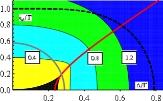
Figure 1: Contour plot of the positive imaginary part of the dimensionless root Im$[y_{1}]/\Gamma=\frac{\sqrt{3}}{2\Gamma}(S-T)$. The black area corresponds to the region where all three roots are real. The red line corresponds to $R=0$ and the gray line to $Q=0$. The black dashed curve shows $Im[z_{1}]=-Re[z_{1}]$.

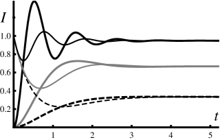
Figure 2: Plot of the current $I(t)$ in Eq. 23 when $\Gamma=1$ and $\epsilon_{d}=0$. The black line corresponds to the parameter $\Delta=3$, the gray line to $\Delta=1$, and the black dashed line to $\Delta=0.5$. Thick lines correspond to the initially empty QD, thin lines to the evolution starting from the zero Bloch vector.

The three roots are

$$y_{l}=e^{2/3\pi il}S+e^{-2/3\pi il}T\ ,$$ (18)

where $l=0,~{}1,~{}2$ and

$$S=\left(R+\sqrt{Q^{3}+R^{2}}\right)^{1/3}\text{ and }T=-\frac{Q}{S}\ .$$ (19)

Here the function $\ Z^{1/3}$ of the complex variable $Z$ is determined in the conventional way with the cut $Z\in\{-\infty,0\}$. If the discriminant is positive: $Q^{3}+R^{2}>0$, $S$ and $T$ are real positive and negative, respectively. Therefore, the root $y_{0}$ is real and the two others $y_{1,2}$ are complex conjugates of each other. In the case of $Q^{3}+R^{2}<0$, $S$ and $T$ are also complex conjugate. Hence, all three roots are real. In this case the oscillatory behavior does not occur. This parametric area of triangular form is depicted as black in Fig. 1. Its three vertices have coordinates (0,0), (1/4,0) and ($\sqrt{2/27},\sqrt{1/27}$).

Oscillatory transient current - With $Q^{3}+R^{2}>0$ we find from Eqs. (11) and (15) that

$$I(t) =I_{0}-\Gamma\left\{r_{0}\cdot e^{-G_{0}t}+2\text{Re}\left[r_{1}\cdot e^{-(G_{1}-i\omega)t}\right]\right\},$$

$$G_{0} =\frac{4}{3}\Gamma-\gamma_{1}\,,\,G_{1}=\frac{4}{3}\Gamma+\frac{\gamma_{1}}{2}.$$ (20)

Here $\gamma_{1}=\frac{1}{3}(S+T)$ and the second term in Eq. (20 ) describes decaying current oscillations of the frequency $\omega=\frac{\sqrt{3}}{6}(S-T)$. Note that the signs of $\gamma_{1}$ and $R$ coincide. Therefore, above the line $R=0$ in Fig.1 $\gamma_{1}$ is negative and the first term of the current in Eq. (20) vanishes more quickly than the amplitude of the second-term oscillations. Below this line $\gamma_{1}$ is positive and the amplitude of the oscillations vanishes more quickly than the first term. By differentiating Eq. (20) we find the condition for the extrema of the current vs. time as

$$-\frac{r_{0}e^{\frac{3}{2}\gamma_{1}t}}{2|r_{1}|}=\frac{\sqrt{G_{1}^{2}+\omega^{2}}}{G_{0}}\sin(\omega t+\varphi_{r}+\chi),$$ (21)

where $\varphi_{r}$ is the phase of $r_{1}$ and $\chi=\arctan(G_{1}/\omega)$. In the parametric area of $R<0$ this equation shows that the current is an infinitely oscillating function of time, while for $R>0$ the current will have a finite number of oscillations only if $r_{0}/(2|r_{1}|)\exp(3\pi\gamma_{1}/(2\omega))$ is less than the coefficient in front of the sine function on the right-hand side of Eq. (21). This condition is not very restrictive and can be circumvented in general. Indeed, contrary to the frequencies and the amplitude decay rates, the residues $r_{0,1}$ of the function $F(z)$ in Eq. (13) depend on the choice of the initial condition $\mathbf{a}(0)$ for the Bloch vector. We can choose the initial condition by varying $\epsilon_{d}$ and $\Gamma$ to bring the qubit into any desirable stationary state within the time of $\sim 1/\Gamma$ and further use this state as an initial condition to the new transient evolution after abrupt change of these parameters. In particular, by tuning $(\mathbf{f}(z_{0})\cdot\mathbf{a}(0))=(\mathbf{f}(z_{0})\cdot\mathbf{a}(\infty))$ we make $r_{0}$ vanish. Then, as follows from Eq. (21) the transient current is always oscillating outside of the black area in Fig. 1, but the direct visibility of these oscillations imposes a stronger condition that $\omega>G_{1}$ as illustrated below. The border of this area is marked by the black dashed line in Fig. 1.

At the resonance $(\epsilon_{d}=0)$ the root $z_{0}$ of $P(z)$ in Eq. (9) comes as $z_{0}=-\Gamma$. The vector $\mathbf{f}(z_{0})$ is zero and so is $r_{0}$ for any initial condition. The current is infinitely oscillating with the frequency $\omega_{r}=\sqrt{4\Delta^{2}-\Gamma^{2}/4}$ if $\Delta>1/16$ and the decay rate of the oscillations amplitude is $G_{1}=(3/2)\Gamma$. The general expression for the residue $r_{1}$ dependence on the initial conditions in Eq. (20) can be found as

$$r_{1} =\left(1+i\frac{\Gamma}{2\omega_{r}}\right)a_{3}(0)-i\frac{2\Delta}{\omega_{r}}a_{2}(0)$$

$$-\Gamma\frac{2\omega_{r}\Gamma+i(\Gamma^{2}+8\Delta^{2})}{4\omega_{r}(\Gamma^{2}+2\Delta^{2})}\,.$$ (22)

We consider first the experimentally feasible case of the qubit evolution from the initial state corresponding to the empty QD.

The empty QD may be prepared by application of the bias voltage to the emitter to make $\epsilon_{d}\gg\Delta,\Gamma.$ Then the state of the qubit, as follows from Eq. (10), is defined by $a_{1}(0)=a_{2}(0)=0$ and $a_{3}(0)=1$ and corresponds to the zero tunneling current. In the resonance case the substitution of Eq. (22) with these initial conditions into Eq. (20) produces a simple formula for the current oscillations

$$I(t)=I_{0}\left(1-\text{Re}\left[\frac{\omega_{r}-3i\Gamma/2}{\omega_{r}}\cdot\exp[-\frac{3}{2}\Gamma t+i\omega_{r}t]\right]\right).$$ (23)

This current dependence on time is depicted in Fig. 2 by thick lines for three different values of $\Delta$, which correspond to $\omega_{r}=0.8667$ in the case of the dashed line and $\omega_{r}=1.94$ and $\omega_{r}=5.98$ for the gray and black solid lines, respectively. From Eq. (21) we find the extrema of the current in Eq. (23 ) to be exactly at $t_{n}=n\pi/\omega_{r}$. Although the current is always an oscillating function these oscillations become visible first for the gray line in accordance with our criterion $\omega_{r}\geq G_{1}$.

In Fig.2 we also draw three thin lines of the current dependence on time for the same three values of the rate $\Delta$ in the case of the qubit evolution with the initial condition of the zero Bloch vector $\mathbf{a}(0)=0$. The current starts from the finite value $I(0)=\Gamma$. This makes the oscillations of all three lines more visible as their first extremes are located at approximately twice smaller times. This initial state of the qubit can be prepared, in particular, by making the collector tunneling rate $\Gamma$ infinitely small at the resonance. It also could be reached through thermodynamical equilibration of the qubit with the high temperature emitter in the absence of tunneling between QD and the collector due to by some slow dissipation processes unaccounted for in our model. We have performed our calculations in dimensionless units with $\hbar=1$ and $e=1$. In the experiment lar ; lar1 the collector tunneling rate is $\Gamma\approx 0.1meV$ and the parameter $\Delta\approx 0.016meV$. This corresponds to the stationary current $I_{0}\approx 1.2nA$. To observe the regime of oscillations as shown in Fig. 2 (gray line) one can take a heterostructure with $\Gamma=\Delta$. For example, with $\Gamma=\Delta=0.01meV$ the stationary current is $I_{0}=1.62nA$. The unit of time $t$ in Fig. 2 for this value of $\Gamma$ is equal to $65.8ps$.

In conclusion, the spinless electrons tunneling through an interacting resonant level of a QD into an empty collector has been studied in the especially simple, but realistic system, in which all sudden variations in charge of the QD are effectively screened by a single tunneling channel of the emitter. Making use of the exact solution to this model, we have demonstrated that the FES in the tunneling current dependence on voltage should be accompanied by oscillations of the time-dependent transient tunneling current in a wide range of the model parameters. In particular, they occur if the emitter tunneling coupling $\Delta$ or the absolute value of the resonant level energy $|\epsilon_{d}|$ are large enough in comparison to the collector tunneling rate $\Gamma$ and either $\Delta>\Gamma/4$ or $\epsilon_{d}^{2}>\Gamma^{2}/27$ holds. These oscillations result from the emergence of the qubit composed of electron-hole pair at the QD and its coherent dynamics. The qubit can be manipulated by changing voltage and the tunneling rates in the system.

Acknowledgment - The work was supported by the Foundation for Science and Technology of Portugal and by the European Union Seventh Framework Programme (FP7/2007-2013) under grant agreement n^o PCOFUND-GA-2009- 246542 and Research Fellowship SFRH/BI/52154/2013. .

References

- (1) G. D. Mahan, Phys. Rev. 163, 612 (1967).
- (2) P. Nozieres and C. T. de Dominicis, Phys. Rev. 178, 1097 (1969).
- (3) D. A. Abanin and L. S. Levitov, Phys. Rev. Lett. 94, 186803(2005).
- (4) P. H. Citrin, Phys. Rev. B 8, 5545 (1973).
- (5) P. H. Citrin, G. K. Wertheim, and Y. Baer, Phys. Rev. B 16, 4256 (1977).
- (6) K. A. Matveev and A. I. Larkin, Phys. Rev. B 46, 15337 (1992).
- (7) I. Hapke-Wurst, U. Zeitler, H. Frahm, A. G. M. Jansen, R. J. Haug, and K. Pierz, Phys. Rev. B 62, 12621 (2000).
- (8) H. Frahm, C. von Zobeltitz, N. Maire, and R. J. Haug, Phys. Rev. B 74, 035329 (2006).
- (9) N. Maire, F. Hohls, T. Lüdtke, K. Pierz, and R. J. Haug, Phys. Rev. B 75, 233304 (2007).
- (10) M. Ruth, T. Slobodskyy, C. Gould, G. Schmidt, and L. W. Molenkamp, Applied Physics Letters 93, 182104 (2008).
- (11) A. J. Leggett et al., Rev. Mod. Phys. 59, 1 (1987).
- (12) O. Katsuba and H. Schoeller, Phys. Rev. B 87, 201402(R) (2013).
- (13) K. Schotte and U. Schotte, Phys. Rev. 182, 479 (1969).
- (14) H.T. Imam, V.V. Ponomarenko, and D.V. Averin, Phys. Rev. 50, 18288 (1994).
- (15) I.A. Larkin, E.E. Vdovin, Yu.N. Khanin, S. Ujevic and M. Henini, Phys. Scripta, 82, 038106, (2010).
- (16) N. Jacobson, Basic algebra 1 (2nd ed.), Dover, (2009), ISBN 978-0-486-47189-1
- (17) I.A. Larkin, Yu.N. Khanin, E.E. Vdovin, S. Ujevic and M. Henini, J. Phys.: Conf. Ser. 456, 012024, ( 2013).