A high-order spectral deferred correction strategy for low Mach number flow with complex chemistry

Abstract.

We present a fourth-order finite-volume algorithm in space and time for low Mach number reacting flow with detailed kinetics and transport. Our temporal integration scheme is based on a multi-implicit spectral deferred correction (MISDC) strategy that iteratively couples advection, diffusion, and reactions evolving subject to a constraint. Our new approach overcomes a stability limitation of our previous second-order method encountered when trying to incorporate higher-order polynomial representations of the solution in time to increase accuracy. We have developed a new iterative scheme that naturally fits within our MISDC framework that allows us to simultaneously conserve mass and energy while satisfying on the equation of state. We analyse the conditions for which the iterative schemes are guaranteed to converge to the fixed point solution. We present numerical examples illustrating the performance of the new method on premixed hydrogen, methane, and dimethyl ether flames.

Keywords: low Mach number combustion, spectral deferred corrections, fourth-order spatiotemporal discretisations, flame simulations, detailed chemistry and kinetics

1. Introduction

A broad range of problems in fluid mechanics are characterized by dynamics with low Mach number. In such systems, acoustic propagation typically has negligible impact on the system state. Low Mach number models exploit this separation between flow and acoustic dynamics by analytically removing sound waves from the system entirely. In the approximation, pressure formally becomes an elliptic field with global coupling, and the set of conservation laws take the form of a coupled differential-algebraic system. Numerically, the low Mach number model can be time-advanced on the scales of (slow) advection processes. However, such schemes can be quite complex to implement for multidimensional, time-dependent flows. Moreover, there are many low Mach number systems where the chemical and diffusive dynamics can operate on time scales that can be much faster than the advection; practically, the realizable time step becomes limited by the extent to which these processes are properly coupled during time-advance. In this paper, we develop a highly efficient low Mach number integration strategy that is fourth-order in space and time, while simultaneously respecting the nonlinear coupling of all the processes. We compare this new algorithm to earlier versions that are both low order and less efficiently coupled in order to demonstrate the significant improvements afforded by the new scheme.

For smooth test problems, characterizing the convergence behavior of a numerical integration algorithm is straighforward; with increasing resolution higher-order spatial and temporal discretization methods will eventually provide more accurate solutions than lower-order methods. For more complex problems, however, we cannot a priori assume that the minimum resolution falls within the asymptotic range of the methods, and therefore that higher-order methods are always more efficient. In simple inert flow applications, we can appeal to Reynolds numbers and Kolmogorov scales to develop absolute accuracy requirements. As an example of this approach, it was demonstrated in Reference [1] that for low-speed turbulent flows high-order temporal and spatial discretisations outperformed comparable second-order schemes, reducing by a factor of two in each dimension the size of the computational mesh needed to resolve turbulent flows at a given Reynolds number. For reacting low Mach number flows, resolution requirements are additionally determined by the need to accurately resolve the chemical dynamics, and to capture the coupling between chemistry and the transport processes in the fluid.

In [2] a second-order method for reacting low Mach number flow with detailed kinetics and transport is introduced. The low Mach number model is a set of differential algebraic equations representing coupled advection, diffusion, and reaction processes that evolve subject to a constraint. One approach to solving such a system is to recast the equation of state as a constraint on the velocity divergence that determines the evolution of the thermodynamic state. The numerical method in [2] uses a finite-volume discretisation in space and a time-stepping method based on a variant of Spectral Deferred Corrections (SDC) [3]. SDC is an iterative method for ordinary differential equations that has the appealing feature that variants of arbitrarily high order can be constructed from relatively simple lower-order methods. In [4], a semi-implicit variant method (SISDC) is introduced for ODEs with both stiff and non-stiff processes, such as advection-diffusion systems. The correction equations for the non-stiff terms are discretised explicitly, whereas the stiff corrections are treated implicitly. Bourlioux, Layton, and Minion [5, 6] introduce a multi-implicit SDC approach (MISDC) for PDEs with advection, diffusion, and reaction processes. The advection correction equation is treated explicitly, while the diffusion and reaction corrections are treated implicitly and independently.

In [2], a modified MISDC method is employed where the reaction correction equation is solved with a separate ODE solver in a manner similar to the classic defect correction schemes [7]. This allows the advection, diffusion, and reaction terms to be decoupled in the time step while retaining second-order accuracy in time. In addition, the tighter coupling of the terms in the deferred corrections as compared to classical Strang splitting results in a reduction of computational effort in the reaction solves because of smaller artificially stiff transients caused by operator splitting. In this paper, we extend the results in [2] to construct a method which is fourth-order in space and time for realistic test problems in one dimension. The algorithm is closer in spirit to the original MISDC [5, 6] approach, and we present an analysis demonstrating why the approach in [2] is ill-suited for extension to higher-order in time.

In this paper we also develop a new technique where we evolve mass and energy using conservation equations while satisfying the equation of state. Our approach is based on previous ‘volume discrepancy’ approaches [8, 9, 2] where the divergence constraint is modified to drive the state variables toward equilibrium with the ambient pressure, but now leverages the iterative nature of our SDC algorithm to essentially eliminate thermodynamic drift.

The rest of this paper is organised as follows. In Section 2 we review the low Mach number equation set. In Section 3 we review the MISDC methodology, present detailed convergence analysis of a fourth-order variant, and discuss the implementation of this method for a model problem. In Section 4 we present our new volume discrepancy approach, and describe the spatial and temporal discretisation for the full low Mach number reacting flow equations. In Section 5 we present results for our model problem as well as several laminar flames with detailed kinetics and transport. We summarise and conclude in Section 6.

2. Low Mach Number Equation Set

In the low Mach number regime, the characteristic fluid velocity is small compared to the sound speed (typically the Mach number is $M=U/c\sim\mathcal{O}(0.1)$ or smaller), and the effect of acoustic wave propagation is unimportant to the overall dynamics of the system. In a low Mach number numerical method, acoustic wave propagation is mathematically removed from the equations of motion, allowing for a time step based on an advective CFL condition,

(1) $$\max_{\bf i}\frac{|U_{i}|\Delta t}{\Delta x}\leq\sigma;\quad 0\leq\sigma\leq 1,$$

where $\sigma$ is the advective CFL number, the maximum is taken over all grid cells, $\Delta x$ is the grid spacing, and $U_{i}$ is the fluid velocity in cell $i$. Thus, this approach leads to a $\sim 1/M$ increase in the allowable time step over an explicit compressible approach. Note that a low Mach number method does not enforce that the Mach number remain small, but rather is suitable for flows in this regime.

In this paper, we use the low Mach number equation set from [9, 2], which is based on the model for low Mach number combustion introduced by Rehm and Baum [10] and rigorously derived from an asymptotic analysis by Majda and Sethian [11]. We consider a gaseous mixture ignoring Soret and Dufour effects, and assume a mixture model for species diffusion [12, 13]. The resulting equations are a set of partial differential equations representing coupled advection, diffusion, and reaction processes that are closed by an equation of state. The equation of state takes the form of a divergence constraint on the velocity, which is derived by differentiating the equation of state in the Lagrangian frame of the moving fluid and enforcing that the thermodynamic pressure remains constant. Physically this manifests itself as instantaneous acoustic equilibration to the constant thermodynamic pressure $p_{0}$ (we only consider open containers in non-gravitationally stratified environments). In the model, sound waves are analytically eliminated from our system while retaining local compressibility effects due to reactions, mass diffusion, and thermal diffusion.

Using the notation in [9, 2], the evolution equations for the thermodynamic variables, $(\rho,{\bf Y},h)$, are instantiations of mass and energy conservation:

(2) $$\frac{\partial(\rho Y_{j})}{\partial t} = -\nabla\cdot(U\rho Y_{j})+\nabla\cdot\rho\mathcal{D}_{j}\nabla Y_{j}+\dot{\omega}_{j},$$

(3) $$\frac{\partial(\rho h)}{\partial t} = -\nabla\cdot(U\rho h)+\nabla\cdot\frac{\lambda}{c_{p}}\nabla h+\sum_{j}\nabla\cdot h_{j}\left(\rho\mathcal{D}_{j}-\frac{\lambda}{c_{p}}\right)\nabla Y_{j},$$

where $\rho$ is the density, ${\bf Y}=(Y_{1},\ldots,Y_{N})$ are the species mass fractions, $\mathcal{D}_{j}({\bf Y},T)$ are the species mixture-averaged diffusion coefficients, $T$ is the temperature, $\dot{\omega}_{j}({\bf Y},T)$ is the production rate for $\rho Y_{j}$ due to chemical reactions, $h=\sum_{j}Y_{j}h_{j}$ is the enthalpy with $h_{j}=h_{j}(T)$ the enthalpy of species $j$, $\lambda({\bf Y},T)$ is the thermal conductivity, and $c_{p}=\sum_{j}Y_{j}dh_{j}/dT$ is the specific heat at constant pressure. Our definition of enthalpy includes the standard enthalpy of formation, so there is no net change to $h$ due to reactions. These evolution equations are closed by an equation of state, which states that the thermodynamic pressure remain constant,

(4) $$p_{0}=\rho\mathcal{R}T\sum_{j}\frac{Y_{j}}{W_{j}},$$

where $\mathcal{R}$ is the universal gas constant and $W_{j}$ is the molecular weight of species $j$. A property of multicomponent diffusive transport is that the species diffusion fluxes must sum to zero in order to conserve total mass. For mixture models such as the one considered here, $\Gamma_{j}\equiv\rho\mathcal{D}_{j}\nabla Y_{j}$, and that property is not satisfied in general. Our approach is to identify a dominant species, in this case N₂, and define $\Gamma_{{\rm N}_{2}}=-\sum_{j\neq{\rm N}_{2}}\Gamma_{j}$. Summing the species equations and noting that $\sum_{j}Y_{j}=1$ and $\sum_{j}\dot{\omega}_{j}=0$, we see that (2) implies the continuity equation,

(5) $$\frac{\partial\rho}{\partial t}=-\nabla\cdot(U\rho).$$

Equations (2), (3), and (4) form the system that we would like to solve. Rather than directly attacking this system of constrained differential algebraic equations, we use a standard approach of recasting the equation of state as a divergence constraint on the velocity field. The constraint is derived by taking the Lagrangian derivative of equation (4), enforcing that $p_{0}$ remain constant, and substituting in the evolution equations for $\rho,{\bf Y}$, and $T$ as described in [8, 9]. This leads to the constraint,

(6) $$\nabla\cdot U = \frac{1}{\rho c_{p}T}\left(\nabla\cdot\lambda\nabla T+\sum_{j}\Gamma_{j}\cdot\nabla h_{j}\right)$$

$$+\frac{1}{\rho}\sum_{j}\frac{W}{W_{j}}\nabla\cdot\Gamma_{j}+\frac{1}{\rho}\sum_{j}\left(\frac{W}{W_{j}}-\frac{h_{j}}{c_{p}T}\right)\dot{\omega}_{j}\equiv S,$$

where $W=(\sum_{j}Y_{j}/W_{j})^{-1}$ is the mixture-averaged molecular weight. This constraint is a linearised approximation to the velocity field required to hold the thermodynamic pressure equal to $p_{0}$ subject to local compressibility effects due to reaction heating, compositional changes, and thermal diffusion.

In two and three dimensions there is an evolution equation for velocity. In second-order schemes for incompressible and low Mach number flow, the velocity field is evolved subject to this evolution equation, and later projected onto the vector space that satisfies the divergence constraint. In one dimension, the velocity field is uniquely specified by (6) and the inflow boundary condition, and therefore no projection is necessary. We are currently exploring ways to extend the higher-order methodologies in this paper to multiple dimensions subject to the divergence constraint.

3. Multi-Implicit SDC

Here we review the SDC and MISDC methodology. SDC methods for ODEs are introduced in Dutt et al. [3]. The basic idea of SDC is to write the solution of an ODE

(7) $$\phi_{t}(t) = F(t,\phi(t)),\qquad t\in[t^{n},t^{n}+\Delta t];$$

(8) $$\phi(t^{n}) = \phi^{n},$$

as the associated integral equation,

(9) $$\phi(t)=\phi^{n}+\int_{t^{n}}^{t}F(\tau,\phi(\tau))~{}d\tau.$$

We will suppress explicit dependence of $F$ and $\phi$ on $\tau$ for notational simplicity. Given an approximation $\phi^{(k)}(t)$ to $\phi(t)$, we use an update equation to iteratively improve the solution,

(10) $$\phi^{(k+1)}(t)=\phi^{n}+\int_{t^{n}}^{t}\left[F(\phi^{(k+1)})-F(\phi^{(k)})\right]d\tau+\int_{t^{n}}^{t}F(\phi^{(k)})~{}d\tau,$$

where a low-order discretisation (e.g., forward or backward Euler) is used to approximate the first integral and a higher-order quadrature is used to approximate the second integral. By doing so, each iteration in $k$ improves the overall order of accuracy of the approximation by one, up to the order of accuracy of the underlying quadrature rule used to evaluate the second integral.

For a given timestep, we subdivide the interval $[t^{n},t^{n}+\Delta t]$ into $M$ subintervals, with $M+1$ temporal nodes given by

$$t^{n}=t^{n,0}<t^{n,1}<\ldots<t^{n,M}=t^{n}+\Delta t\equiv t^{n+1}.$$

For notational simplicity we will write $t^{m}=t^{n,m}$. We choose the temporal nodes $t^{m}$ to be the appropriate Gauss-Lobatto quadrature points, though other choices are available [14]. We also denote the substep time interval by $\Delta t^{m}=t^{m+1}-t^{m}$. We let $\phi^{m,(k)}$ represent the $k^{\rm th}$ iterate of the solution at the $m^{\rm th}$ temporal node.

Bourlioux et al. [5] and Layton and Minion [6] introduce a variant of SDC, referred to as MISDC, in which $F$ is decomposed into distinct processes with each treated sequentially with an appropriate explicit or implicit temporal discretisation. An important difference between MISDC methods and operator splitting methods such as Strang splitting is that MISDC methods iteratively couple all physical processes together by including the effects of each process during the integration of any particular process. This is in contrast to Strang splitting, where each process is discretised in isolation, ignoring the effects of other processes. Here, we write

(11) $$\phi_{t}=F_{A}(\phi)+F_{D}(\phi)+F_{R}(\phi)\equiv F(\phi),$$

where $F_{A}$, $F_{D}$, and $F_{R}$ represent the advection, diffusion, and reaction processes respectively. In our problems of interest, diffusion and reactions operate on fast time scales compared to advection. Thus, we seek an explicit treatment of advection and an implicit treatment of reactions and diffusion.

We begin by initialising the solution at all temporal nodes to the solution at $t^{n}$, i.e., $\phi^{m,(0)}=\phi^{n},$ for all $m\in[0,M]$. We seek to compute the next iterate of the solution, $\phi^{m,(k+1)}$ for all $m$ given that we know $\phi^{m,(k)}$ for all $m$. We do this by noting that $\phi^{0,(k)}=\phi^{n}$ for all $k\in[0,K]$, and then solving for each $\phi^{m+1,(k+1)}$ from $m=0$ to $M-1$ using the following sequence:

(12) $$\phi_{\rm A}^{m+1,(k+1)}=\phi^{m,(k+1)}+\int_{t^{m}}^{t^{m+1}}\left[F_{A}(\phi_{\rm A}^{(k+1)})-F_{A}(\phi^{(k)})\right]dt+\int_{t^{m}}^{t^{m+1}}F(\phi^{(k)})dt,$$

(13) $$\phi_{\rm AD}^{m+1,(k+1)}=\phi^{m,(k+1)} + \int_{t^{m}}^{t^{m+1}}\left[F_{A}(\phi_{\rm A}^{(k+1)})-F_{A}(\phi^{(k)})+F_{D}(\phi_{\rm AD}^{(k+1)})-F_{D}(\phi^{(k)})\right]dt$$

$$+ \int_{t^{m}}^{t^{m+1}}F(\phi^{(k)})dt,$$

$$\phi^{m+1,(k+1)}=\phi^{m,(k+1)} + \int_{t^{m}}^{t^{m+1}}\left[F_{A}(\phi_{\rm A}^{(k+1)})-F_{A}(\phi^{(k)})+F_{D}(\phi_{\rm AD}^{(k+1)})-F_{D}(\phi^{(k)})\right.$$

$$\hskip 36.135pt\left.+F_{R}(\phi^{(k+1)})-F_{R}(\phi^{(k)})\right]dt+\int_{t^{m}}^{t^{m+1}}F(\phi^{(k)})dt.$$

Once $\phi^{(k+1)}$ is known at all temporal nodes $m$, the entire process can be repeated to compute the solution at all temporal nodes for the next iteration in $k$. By using first-order discretisations in time for the first integrals in (12), (13), and (LABEL:eq:MISDC_ADR), and using higher-order quadrature to evaluate the second integrals, the overall accuracy of the solution for each $k$ iterate is increased by 1, up to the order of the quadrature rule used to evaluate the second integral over the entire time step.

In this case, if we use forward Euler to discretise advection, and backward Euler to discretise diffusion and reactions, we note that $\phi_{\rm A}^{m+1,(k+1)}$ does not need to be computed and the update consists of the following two sequential discretisations of equations (13) and (LABEL:eq:MISDC_ADR):

(15) $$\begin{aligned} \phi^{m+1,(k+1)}_{\rm AD}=\phi^{m,(k+1)}+\Delta t^{m}\Big{[}&F_{A}(\phi^{m,(k+1)})-F_{A}(\phi^{m,(k)})\\ +&F_{D}(\phi_{\rm AD}^{m+1,(k+1)})-F_{D}(\phi^{m+1,(k)})\Big{]}+I_{m}^{m+1}\left[F(\phi^{(k)})\right],\end{aligned}$$

(16) $$\begin{aligned} \phi^{m+1,(k+1)}=\phi^{m,(k+1)}+\Delta t^{m}\Big{[}&F_{A}(\phi^{m,(k+1)})-F_{A}(\phi^{m,(k)})\\ +&F_{D}(\phi_{\rm AD}^{m+1,(k+1)})-F_{D}(\phi^{m+1,(k)})\\ +&\left.F_{R}(\phi^{m+1,(k+1)})-F_{R}(\phi^{m+1,(k)})\right]+I_{m}^{m+1}\left[F(\phi^{(k)})\right].\end{aligned}$$

The second integrals in (13) and (LABEL:eq:MISDC_ADR) have been replaced with numerical quadrature integrals over the substep, denoted $I_{m}^{m+1}$. We note that in [5] it was demonstrated that integration errors can be reduced by further subdividing the $M$ subintervals into additional nested subintervals to treat fast-scale processes, such as diffusion and/or reactions. Here, we choose to not further subdivide beyond the original $M$ subintervals, so that we stay faithful to the iterative scheme described by (15) and (16). Our results demonstrate we can simulate complex flames using an advective CFL of $\sigma\sim 0.25$ without substepping diffusion or reactions. Also, we note that for an evolution equation containing only advection (such as density), it is sufficient to use only (12) to iteratively correct the solution, with associated discretisation,

(17) $$\phi^{m+1,(k+1)}=\phi^{m,(k+1)}+\Delta t^{m}\left[F_{A}(\phi^{m,(k+1)})-F_{A}(\phi^{m,(k)})\right]+I_{m}^{m+1}\left[F(\phi^{(k)})\right].$$

In [2], we developed a hybrid MISDC/classical deferred correction scheme to solve the low Mach number equations. The departure from the MISDC formulation as originally proposed in [5] occurred when taking the time-derivative of the reaction correction equation, given by (LABEL:eq:MISDC_ADR) in this paper and equation (24) in [2], assuming that the iteratively-lagged reaction terms cancelled, and opting to solve the ODE in equation (25) in [2] instead of equation (16) in this paper. We then posited that higher-order temporal integration could be achieved by using higher-order polynomial representations of advection and diffusion during the reaction ODE step. In practice, we observed instability whenever polynomials of degree greater than zero were used, so we used a piecewise constant, time-centred representation of advection and diffusion. In Appendix A we present an analysis of the convergence of the numerical method in [2], and demonstrate that the generalisation to higher-order polynomial representations of advection and diffusion results in highly unfavourable stability properties. In light of this, the MISDC approach in this paper stays true to the MISDC approach in [5]. In the next Section we analyse the new method, demonstrating convergence in the fourth-order case.

3.1. Convergence Analysis of Fourth-Order MISDC

The weakly coupled set of equations (12), (13), and (LABEL:eq:MISDC_ADR) are chosen such that successive iterations are intended to converge to a fixed-point solution by sending the splitting error to zero. In order for the iterations to converge, we must clearly have

(18) $$\left|\phi^{m,(k+1)}-\phi^{m,(k)}\right|\to 0\quad\text{as $k\to\infty$}.$$

In order to study this convergence condition, we consider the linear ODE

(19) $$\phi_{t}=a\phi+d\phi+r\phi\equiv F(\phi).$$

The scalar quantities $a$, $d$, and $r$ will be proxies for our treatment of advection, diffusion, and reaction in the full low Mach number code. We can solve this differential equation with fourth-order accuracy, according to the prescription described above. We choose three Gauss-Lobatto nodes,

(20) $$t^{n,0}=t^{n},\qquad t^{n,1}=t^{n}+\Delta t/2,\qquad t^{n,2}=t^{n+1}=t^{n}+\Delta t.$$

As before, we denote $t^{n,m}=t^{m}$. The quadrature $I_{m}^{m+1}$ can then be computed by means of integrating the interpolating quadratic, obtaining the following formulas.

(21) $$I_{0}^{1}(F) =\frac{\Delta t}{24}\left(5F\left(t^{0}\right)+8F\left(t^{1}\right)-F\left(t^{2}\right)\right),$$

(22) $$I_{1}^{2}(F) =\frac{\Delta t}{24}\left(-F\left(t^{0}\right)+8F\left(t^{1}\right)+5F\left(t^{2}\right)\right).$$

Given the solution at the beginning of a time step, $\phi^{n}$, we compute the approximate solution at $t=t^{n}+\Delta t$ as follows. Initialising $\phi^{m,(0)}=\phi^{n}$ for all $m$ and $\phi^{0,(k)}=\phi^{n}$ for all $k$, we compute each successive iterate using equations (15) and (16):

(23) $$\phi^{m+1,(k+1)}_{\rm AD}=\phi^{m,(k+1)} + \Delta t^{m}\left[a\phi^{m,(k+1)}-a\phi^{m,(k)}+d\phi_{\rm AD}^{m+1,(k+1)}-d\phi^{m+1,(k)}\right]$$

$$+I_{m}^{m+1}\left[F(\phi^{(k)})\right],$$

(24) $$\phi^{m+1,(k+1)}=\phi^{m,(k+1)} + \Delta t^{m}\left[a\phi^{m,(k+1)}-a\phi^{m,(k)}\right.+d\phi_{\rm AD}^{m+1,(k+1)}-d\phi^{m+1,(k)}$$

$$+\left.r\phi^{m+1,(k+1)}-r\phi^{m+1,(k)}\right]+I_{m}^{m+1}\left[F(\phi^{(k)})\right],$$

at each temporal node $t^{m}$. Expanding these expressions, we can write

(25) $$\phi^{2,(k+1)}-\phi^{2,(k)} =c_{1}\left(\phi^{1,(k)}-\phi^{1,(k-1)}\right)+c_{2}\left(\phi^{2,(k)}-\phi^{2,(k-1)}\right),$$

where

(26) $$c_{1} =\tfrac{8\Delta t(\Delta t(a^{2}-d^{2}+dr-r^{2})+a+d+r)}{3(d\Delta t-2)^{2}(r\Delta t-2)^{2}},$$

(27) $$c_{2} =\tfrac{\Delta t(-16(d+r)-a^{2}\Delta t+a(8-6(d+r)\Delta t+3dr\Delta t^{2})+\Delta t(7r^{2}+dr(26-9r\Delta t)+d^{2}(7+3r\Delta t(r\Delta t-3)))}{3(d-2)^{2}(r-2)^{2}}.$$

Similar expressions can be derived for the difference $\phi^{1,(k+1)}-\phi^{1,(k)}$. We can therefore conclude that

$$\left|\phi^{1,(k+1)}-\phi^{1,(k)}\right| \leq\alpha\left|\phi^{1,(k)}-\phi^{1,(k-1)}\right|+\beta\left|\phi^{2,(k)}-\phi^{2,(k-1)}\right|,$$

$$\left|\phi^{2,(k+1)}-\phi^{2,(k)}\right| \leq\gamma\left|\phi^{1,(k)}-\phi^{1,(k-1)}\right|+\delta\left|\phi^{2,(k)}-\phi^{2,(k-1)}\right|,$$

where $\alpha,\beta,\gamma,$ and $\delta$ are algebraic expressions in terms of $a,d,r,$ and $\Delta t$. We see that a sufficient condition for successive iterations to converge is the condition $\alpha,\beta,\gamma,\delta<1$. In other words, we define

$$\theta(a,d,r,\Delta t)=\max\{\alpha,\beta,\gamma,\delta\},$$

and require $\theta<1$.

It is possible to compare the sets of parameters $a$, $d$, $r$, and $\Delta t$ that result in $\theta<1$. For the sake of comparison, we set $a=0$, and plot the regions $(d\Delta t,r\Delta t)\in\mathbb{R}^{2}$ such that $\theta<1$ in Figure 1. Comparing the current method to that proposed in [2] and analysed in Appendix A, we observe that the region of convergence of the current method encompasses a much larger range of parameters.

(a) New MISDC method

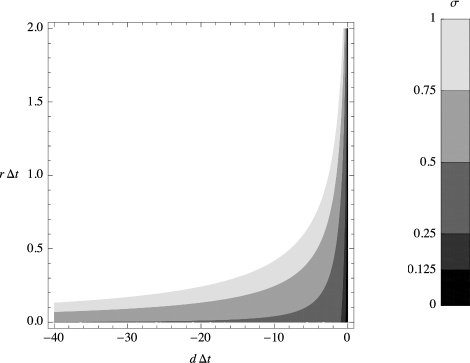
(b) Previous proposed method

Figure 1. Convergence regions $(d\Delta t,r\Delta t)\in\mathbb{R}^{2}$

The parameters $a$, $d$ are chosen to represent the eigenvalues of the advection and diffusion operators, respectively. Therefore, $a$ can be considered to scale like $1/\Delta x$, and $d$ to scale like $1/\Delta x^{2}$. We also make the ansatz of a linear CFL, i.e. $\Delta t=\lambda\Delta x$ for some $\lambda$. The reaction parameter, $r$, is independent of $\Delta x$.

We therefore write $a=\tilde{a}/\Delta x$, and $d=\tilde{d}/\Delta x^{2}$, where $\tilde{a}$ and $\tilde{d}$ are given parameters. A sufficient condition for the iterative scheme to converge as we send $\Delta x$ to zero is

$$\lim_{\Delta x\to 0}\theta(\tilde{a}/\Delta x,\tilde{d}/\Delta x^{2},r,\lambda\Delta x)<1.$$

Calculating the limits explicitly, we see that

$$\lim_{\Delta x\to 0}\alpha =\frac{1}{12}, \lim_{\Delta x\to 0}\beta =\frac{1}{3},$$

$$\lim_{\Delta x\to 0}\gamma =\frac{2}{3}, \lim_{\Delta x\to 0}\delta =\frac{7}{12},$$

and therefore $\lim_{\Delta x\to 0}\theta=2/3$. We can conclude that the fourth-order MISDC method described above is convergent in the limit as $\Delta x$ tends to zero. This is in contrast to the method described in [2], for which the convergence analysis is performed in Appendix A. We verify fourth-order accuracy for this approach using a test problem described in Section 5.1.

4. Numerical Methodology

For the full low Mach number system we consider a one-dimensional finite volume formulation with constant grid spacing $\Delta x$. We describe the fourth-order MISDC temporal integration strategy in detail in Section 4.2. We describe the fourth-order spatial discretisation in detail in Section 4.3.

4.1. A New Approach for Constrained Evolution

A major hurdle in the development of low Mach number methodologies for complex flows is the issue that the mass and energy fields updated with conservation equations will, in general, fail to satisfy the equation of state. We define $p_{\rm EOS}$ as the thermodynamic pressure, computed directly with the equation of state using variables updated from the conservation equations (i.e., the right-hand-side of equation (4)), and $p_{0}$ as the (constant) ambient pressure. Our approach of recasting the equation of state as a divergence constraint on the velocity field is designed to constrain the evolution of the thermodynamic state such that $p_{\rm EOS}$ remains approximately $p_{0}$. However, our formulation represents a linearisation, or tangent-plane approximation, to the dynamics of the system. Since the equation of state is nonlinear, a small drift between $p_{\rm EOS}$ and $p_{0}$ will be observed, and indeed will grow over time.

One standard approach to resolve this issue [15, 16] is to evolve all the thermodynamic variables but one (typically the energy or total density field) with conservation equations, and then use the equation of state to compute the remaining variable so that $p_{\rm EOS}=p_{0}$ identically. A serious disadvantage of this approach is that it fails to conserve mass, energy, or both. In previous works [8, 9, 2] we introduced an alternative ’volume discrepancy’ approach that drives $p_{\rm EOS}$ toward $p_{0}$ in a way that is conservative while maintaining the drift below a few percent. In this paper, we exploit the iterative nature of the MISDC advance in order to develop an improved volume discrepancy correction.

Similar to our previous volume discrepancy approach, the constraint equation is modified to allow additional expansion of the fluid, accounting for the thermodynamic drift. However, here the increment is adjusted at each MISDC iteration, allowing us to iteratively adjust the driving terms so that drift effectively becomes zero at the end of each time step. In order to construct this iteration, we return to the derivation of the velocity constraint. First, the equation of state, $p=p(\rho,T,{\bf Y})$, is differentiated in the Lagrangian frame of the moving fluid,

(28) $$\frac{Dp}{Dt}=p_{\rho}\frac{D\rho}{Dt}+p_{T}\frac{DT}{Dt}+\sum_{j}p_{Y_{j}}\frac{DY_{j}}{Dt},$$

where the following partial derivatives are defined:

(29) $$p_{\rho}=\left.\frac{\partial p}{\partial\rho}\right|_{T,{\bf Y}},\quad p_{T}=\left.\frac{\partial p}{\partial T}\right|_{\rho,{\bf Y}},\quad p_{Y_{j}}=\left.\frac{\partial p}{\partial Y_{j}}\right|_{\rho,T,Y_{k,k\neq j}}.$$

Using continuity, $D\rho/Dt=-\rho\nabla\cdot U$, we rewrite (28) as

(30) $$\nabla\cdot U=\frac{1}{\rho p_{\rho}}\left(-\frac{Dp}{Dt}+p_{T}\frac{DT}{Dt}+\sum_{j}p_{Y_{j}}\frac{DY_{j}}{Dt}\right)$$

Note that equation (30) is analytically equivalent to equation (6) if $Dp/Dt=\delta\chi=0$. Next, rather than setting $Dp/Dt=0$, we approximate at each cell the time derivative, $\delta\chi$, necessary to drive the drift to zero over $\Delta t$, based on current estimates of the advanced state:

(31) $$\delta\chi=\frac{1}{\rho p_{\rho}}\frac{Dp}{Dt}=\frac{1}{p_{0}}\left(\frac{p_{0}-p_{\rm EOS}}{\Delta t}\right).$$

This field is initialised to zero on the first MISDC iteration. After each iteration, equation (31) is used to estimate a new correction (increment to $\delta\chi$) required to drive the drift computed at that iteration to zero, and this is then used in subsequent evaluations of equation (30) for $Dp/Dt$.

The net effect of this iteration is to adjust the advection velocities such that the conservative updates for mass and energy are both rigorously conservative and consistent with the equation of state. For sufficiently resolved flows, this adjustment is small and the overall algorithm exhibits fourth-order accuracy, as demonstrated in the examples that follow.

4.2. Temporal Discretisation

In our fourth-order approach, we use $M=2$ substeps (3 Gauss-Lobatto temporal nodes) and $K\geq 4$ MISDC iterations, but the steps below have been generalised for any number of temporal nodes and MISDC iterations. The steps required to advance the solution from $t^{n}$ to $t^{n+1}$ are as follows:

Set $(\rho h,\rho{\bf Y})^{0,(k)}=(\rho h,\rho{\bf Y})^{n}$ for all $k\in[0,K]$, i.e., the solution at temporal node $m=0$ is a copy of the solution at $t^{n}$ for all MISDC iterations.

Set $(\rho h,\rho{\bf Y})^{m,(0)}=(\rho h,\rho{\bf Y})^{n}$ for all $m\in[1,M]$, i.e., the solution for MISDC iteration $k=0$ is a copy of the solution at $t^{n}$ for all temporal nodes.

We use a sequence of $\delta\chi$ correction terms, one associated with each subinterval denoted $\delta\chi^{m-1:m,(k)}$. Each of these terms modifies the divergence constraint at temporal node $m$ to drive the variables to thermodynamic equilibrium in the next MISDC iteration. We initialise $\delta\chi^{m-1:m,(0)}=0$ for all $m\in[1,M]$.

We compute face-averaged velocities at $t^{n}$ by integrating the constraint

(32) $$\nabla\cdot U^{n}=S^{n}$$

We set $U^{0,(k)}=U^{n}$ for all $k\in[0,K]$.

Next, we explicitly evaluate the right-hand-sides of the species equations (2) and enthalpy equation (3) from the $k=0$ state for all $m\in[0,M]$, noting that these states are all identical at the beginning of the time step. These terms are used to evaluate $I_{m}^{m+1}[F(\phi^{(k)})]$ in the steps below during the first MISDC iteration.

Now we loop over MISDC iterations (in $k$) over each temporal node (in $m$):

for $k=0\text{ \bf to }K-1$ do

     for $m=0\text{ \bf to }M-1$ do

          If $m>0$, correct to the divergence constraint to account for the fact that the $p_{\rm EOS}$ does not match $p_{0}$ in the most recent solution,

(33) $$\delta\chi^{m-1:m,(k+1)}=\delta\chi^{m-1:m,(k)}+\frac{2}{p_{0}}\left(\frac{p_{\rm EOS}^{m,(k+1)}-p_{0}}{\Delta t^{m-1}}\right),$$

          where, again, $p_{\rm EOS}$ is a function of $\rho,{\bf Y},T$ given by the right-hand-side of equation (4). Note, the factor of 2 in (33) reflects that our correction is applied piecewise linearly over the time interval from $t^{m}$ to $t^{m+1}$, with zero increment of $\delta\chi$ at $t^{m}$. We then compute face-averaged velocities, $U^{m,(k+1)}$, by integrating the constraint,

(34) $$\nabla\cdot U^{m,(k+1)}=S^{m,(k+1)}+\delta\chi^{m-1:m,(k+1)}.$$

          (For all $m$) Compute $\rho^{m+1,(k+1)}$ by discretising the continuity equation (5) with the MISDC correction equation for PDEs containing only advection terms (17),

(35) $$\rho^{m+1,(k+1)}=\rho^{m,(k+1)} + \Delta t^{m}\left[-\nabla\cdot(U\rho)^{m,(k+1)}+\nabla\cdot(U\rho)^{m,(k)}\right]$$

$$+ I_{m}^{m+1}\left[-\nabla\cdot(U\rho)^{(k)}\right].$$

          Compute updated mass fractions, $Y_{j,{\rm AD}}^{m+1,(k+1)}$, by discretising the species equations (2) with the MISDC advection-diffusion correction equation (15). This amounts to solving the implicit system,

$$\rho^{m+1,(k+1)}Y_{j,{\rm AD}}^{m+1,(k+1)} =\mathmakebox[2em][l]{(\rho Y_{j})^{m,(k+1)}}$$

$$+\Delta t^{m}\Big{[} -\nabla\cdot(U\rho Y_{j})^{m,(k+1)}+\nabla\cdot(U\rho Y_{j})^{m,(k)}$$

$$+\nabla\cdot\rho^{m+1,(k)}\mathcal{D}_{j}^{m+1,(k)}\nabla Y_{j,{\rm AD}}^{m+1,(k+1)}-\nabla\cdot\Gamma_{j}^{m+1,(k)}\Big{]}$$

(36) $$\mathmakebox[2em][l]{+I_{m}^{m+1}\left[-\nabla\cdot(U\rho Y_{j})+\nabla\cdot\Gamma_{j}+\dot{\omega}\right]^{(k)}.}$$

         Define $\Gamma_{j,{\rm AD}}^{m+1,(k+1)}=\rho^{m+1,(k)}\mathcal{D}_{j}^{m+1,(k)}\nabla Y_{j,{\rm AD}}^{m+1,(k+1)}$.

          Compute updated enthalpy, $h_{\rm AD}^{m+1,(k+1)}$, by discretising the enthalpy equation (3) with the MISDC advection-diffusion correction equation (15). We remark that the differential diffusion terms are treated explicitly in order to avoid a more complicated linear system. This amounts to solving the implicit system,

$$\mathmakebox[2em][l]{\rho^{m+1,(k+1)}h_{\rm AD}^{m+1,(k+1)}=(\rho h)^{m,(k+1)}}$$

$$+\Delta t^{m}\Bigg{[} -\nabla\cdot(U\rho h)^{m,(k+1)}+\nabla\cdot(U\rho h)^{m,(k)}$$

$$+\nabla\cdot\frac{\lambda^{m+1,(k)}}{c_{p}^{m+1,(k)}}\nabla h_{\rm AD}^{m+1,(k+1)}-\nabla\cdot\frac{\lambda^{m+1,(k)}}{c_{p}^{m+1,(k)}}\nabla h^{m+1,(k)}$$

$$+\sum_{j}\nabla\cdot h_{j}^{m,(k+1)}\left(\Gamma_{j}^{m,(k+1)}-\frac{\lambda^{m,(k+1)}}{c_{p}^{m,(k+1)}}\nabla Y_{j}^{m,(k+1)}\right)$$

$$-\sum_{j}\nabla\cdot h_{j}^{m,(k)}\left(\Gamma_{j}^{m,(k)}-\frac{\lambda^{m,(k)}}{c_{p}^{m,(k)}}\nabla Y_{j}^{m,(k)}\right)\Bigg{]}$$

(37) $$\mathmakebox[2em][l]{+I_{m}^{m+1}\left[-\nabla\cdot(U\rho h)+\nabla\cdot\frac{\lambda}{c_{p}}\nabla h+\sum_{j}\nabla\cdot h_{j}\left(\Gamma_{j}-\frac{\lambda}{c_{p}}\nabla Y_{j}\right)\right]^{(k)}.}$$

         

          Note that since there is no contribution due to reactions in the enthalpy update, we can say

(38) $$(\rho h)^{m+1,(k+1)}=\rho^{m+1,(k+1)}h_{\rm AD}^{m+1,(k+1)}.$$

          Next, we solve the reaction correction equation for $(\rho Y_{j})^{m+1,(k+1)}$ using the MISDC advection-diffusion-reaction correction equation (16),

(39) $$(\rho Y_{j})^{m+1,(k+1)} = \mathmakebox[2em][l]{(\rho Y_{j})^{m,(k+1)}}$$

$$+\Delta t^{m}\Big{[}-\nabla\cdot(U\rho Y_{j})^{m,(k+1)}-\nabla\cdot(U\rho Y_{j})^{m,(k)}$$

$$\hskip 36.135pt+\nabla\cdot\Gamma_{j,{\rm AD}}^{m+1,(k+1)}-\nabla\cdot\Gamma_{j}^{m+1,(k)}$$

$$\hskip 36.135pt+\dot{\omega}^{m+1,(k+1)}-\dot{\omega}^{m+1,(k)}\Big{]}$$

$$\mathmakebox[2em][l]{+I_{m}^{m+1}\left[-\nabla\cdot(U\rho Y_{j})+\nabla\cdot\Gamma_{j}+\dot{\omega}\right]^{(k)}.}$$

          See Section 4.2.1 for our solution technique for these nonlinear implicit equations.

         

         

     end for (end loop over temporal nodes $m$)

      Since in general, $p_{\rm EOS}$ at the final temporal node (the “$M,(k+1)$" state) is not in thermodynamic equilibrium with $p_{0}$, we correct the divergence constraint. We do this by incrementing $\delta\chi^{M-1:M,(k+1)}$ using

(40) $$\delta\chi^{M-1:M,(k+1)}=\delta\chi^{M-1:M,(k)}+\frac{2}{p_{0}}\left(\frac{p_{\rm EOS}^{M,(k+1)}-p_{0}}{\Delta t^{M-1}}\right).$$

      Compute $U^{M,(k+1)}$ by integrating the constraint, (41) $$\nabla\cdot U^{M,(k+1)}=S^{M,(k+1)}+\delta\chi^{M-1:M,(k+1)},$$ and evaluate the right-hand-sides of the species equations (2) and enthalpy equation (3) from the ’$M,(k+1)$’ state.

end for (end loop over MISDC iterates $k$)

Advance the solution by setting $(\rho h,\rho{\bf Y})^{n+1}=(\rho h,\rho{\bf Y})^{M,(K)}$.

4.2.1. Solving the Reaction Correction Equations

To solve the reaction correction equations (39) for $(\rho Y_{m})^{m+1,(k+1)}$, we use Newton’s method for this implicit system. Note that since there is no reaction contribution to the enthalpy equation, $(\rho h)^{m+1,(k+1)}$ is already known from (38). Likewise, the density $\rho^{m+1,(k+1)}$ is known from equation (35). The production rates are a function of ${\bf Y}$ and $h$. Writing out the mass fractions ${\bf Y}\equiv(Y_{1},\ldots,Y_{N})$, and the production rates $\dot{\bm{\omega}}\equiv(\dot{\omega}_{1},\ldots,\dot{\omega}_{N})$, equation (39) takes the form of a nonlinear backward Euler-type equation for ${\bf Y}$:

(42) $$\rho^{m+1,(k+1)}{\bf Y}-\Delta t^{m}\dot{\bm{\omega}}({\bf Y})={\bf b}.$$

We use an analytic Jacobian [17] and using the solution from the previous MISDC iterate as an initial guess. The Newton solve has been observed to converge to within tolerance within only a few iterations for all $k$, and in subsequent MISDC iterations, the initial guess improves with each iteration and even fewer Newton iterations are needed. We iterate until the max norm of the residual is less than $10^{-14}$. In our testing, using an even tighter tolerance of $10^{-16}$ did not affect the convergence rates in the significant figures we report below.

4.3. Spatial Discretisation

We use a finite volume discretisation with $n$ cells, indexed from $i=(0,\ldots,n-1)$. We distinguish between three types of quantities. A cell-averaged quantity is denoted by angle brackets,

$$\langle\phi\rangle_{i}\equiv\frac{1}{\Delta x}\int_{x_{i-\frac{1}{2}}}^{x_{i+\frac{1}{2}}}\phi(x)~{}dx.$$

A cell-centred quantity is denoted by a hat, $\widehat{\phi}_{i}\equiv\phi(x_{i})$, and a face-averaged quantity is denoted by a tilde, $\widetilde{\phi}_{i+\frac{1}{2}}\equiv\phi(x_{i+\frac{1}{2}})$. Note that in one dimension, face-averages are simply point values at the endpoints of a cell.

To convert between these values, as well as compute fourth-order gradients, products, and quotients, we rely on standard operations found in the finite volume literature [1, 18, 19, 20]. The fourth-order formulas to convert from cell-averaged to cell-centred, and vice versa, are,

(43) $$\widehat{\phi}_{i} = \langle\phi\rangle_{i}-\frac{1}{24}(\langle\phi\rangle_{i-1}-2\langle\phi\rangle_{i}+\langle\phi\rangle_{i+1}),$$

(44) $$\langle\phi\rangle_{i} = \widehat{\phi}_{i}+\frac{1}{24}(\widehat{\phi}_{i-1}-2\widehat{\phi}_{i}+\widehat{\phi}_{i+1}).$$

We can compute a fourth-order approximation of a quantity at cell faces given either cell-centred values or cell-averaged values using the following stencils:

(45) $$\widetilde{\phi}_{i+\frac{1}{2}} =\frac{-\langle\phi\rangle_{i-1}+7\langle\phi\rangle_{i}+7\langle\phi\rangle_{i+1}-\langle\phi\rangle_{i+2}}{12},$$

(46) $$\widetilde{\phi}_{i+\frac{1}{2}} =\frac{-\widehat{\phi}_{i-1}+9\widehat{\phi}_{i}+9\widehat{\phi}_{i+1}-\widehat{\phi}_{i+2}}{16}.$$

The fourth-order approximation to the gradient at a cell face is

(47) $$\widetilde{\nabla\phi}_{i+\frac{1}{2}}=\frac{\langle\phi\rangle_{i-1}-15\langle\phi\rangle_{i}+15\langle\phi\rangle_{i+1}-\langle\phi\rangle_{i+2}}{12\Delta x}.$$

Given cell-averaged quantities $\langle\phi\rangle_{i}$ and $\langle\psi\rangle_{i}$, we can compute a fourth-order approximation to the cell-average of the product by

(48) $$\langle\phi\psi\rangle_{i}=\langle\phi\rangle_{i}\langle\psi\rangle_{i}+\frac{\Delta x^{2}}{12}\phi^{\rm G}_{i}\psi^{\rm G}_{i}+\mathcal{O}(\Delta x^{4}),$$

where $\phi^{\rm G}_{i}$ and $\psi^{\rm G}_{i}$ are given by the gradient formula, e.g.,

(49) $$\phi^{\rm G}_{i}=\frac{5\langle\phi\rangle_{i-2}-34\langle\phi\rangle_{i-1}+34\langle\phi\rangle_{i+1}-5\langle\phi\rangle_{i+2}}{48\Delta x}.$$

Similarly, we can compute a fourth-order approximation to the cell-average of a quotient by

(50) $$\left\langle\frac{\phi}{\psi}\right\rangle_{i}=\frac{\langle\phi\rangle_{i}}{\langle\psi\rangle_{i}}+\frac{\Delta x^{2}}{12}\left(\frac{\langle\phi\rangle_{i}\left(\psi^{\rm G}_{i}\right)^{2}}{\langle\psi\rangle_{i}^{3}}-\frac{\phi^{\rm G}_{i}\psi^{\rm G}_{i}}{\langle\psi\rangle_{j}^{2}}\right)+\mathcal{O}(\Delta x^{4}).$$

At inflow and outflow, the strategy is to use the boundary condition and four interior data values to extrapolate two ghost cells values to fourth-order accuracy, allowing us to use these same stencils. At inflow, we have the Dirichlet value at the face, $\phi_{b}$. Given cell-averaged data, the ghost cell-averaged values are

(51) $$\langle\phi\rangle_{-1}=\frac{60\phi_{b}-77\langle\phi\rangle_{0}+43\langle\phi\rangle_{1}-17\langle\phi\rangle_{2}+3\langle\phi\rangle_{3}}{12}$$

(52) $$\langle\phi\rangle_{-2}=\frac{300\phi_{b}-505\langle\phi\rangle_{0}+335\langle\phi\rangle_{1}-145\langle\phi\rangle_{2}+27\langle\phi\rangle_{3}}{12}$$

Given cell-centred data, the ghost cell-centred values are

(53) $$\widehat{\phi}_{-1}=\frac{128\phi_{b}-140\widehat{\phi}_{0}+70\widehat{\phi}_{1}-28\widehat{\phi}_{2}+5\widehat{\phi}_{3}}{35}$$

(54) $$\widehat{\phi}_{-2}=\frac{128\phi_{b}-210\widehat{\phi}_{0}+140\widehat{\phi}_{1}-63\widehat{\phi}_{2}+12\widehat{\phi}_{3}}{7}$$

At outflow, we have a homogeneous Neumann condition. Given cell-averaged data, the ghost cell-averaged values are

(55) $$\langle\phi\rangle_{n}=\frac{5\langle\phi\rangle_{n-1}+9\langle\phi\rangle_{n-2}-5\langle\phi\rangle_{n-3}+\langle\phi\rangle_{n-4}}{10}$$

(56) $$\langle\phi\rangle_{n+1}=\frac{-15\langle\phi\rangle_{n-1}+29\langle\phi\rangle_{n-2}-15\langle\phi\rangle_{n-3}+3\langle\phi\rangle_{n-4}}{2}$$

Given cell-centred data, the ghost cell-centred values are

(57) $$\widehat{\phi}_{n}=\frac{17\widehat{\phi}_{n-1}+9\widehat{\phi}_{n-2}-5\widehat{\phi}_{n-3}+\widehat{\phi}_{n-4}}{22}$$

(58) $$\widehat{\phi}_{n+1}=\frac{-135\widehat{\phi}_{n-1}+265\widehat{\phi}_{n-2}-135\widehat{\phi}_{n-3}+27\widehat{\phi}_{n-4}}{22}$$

To compute the advection terms, we use the divergence theorem,

(59) $$\langle\nabla\cdot(U\phi)\rangle_{i}=\frac{\widetilde{U}_{i+\frac{1}{2}}\widetilde{\phi}_{i+\frac{1}{2}}-\widetilde{U}_{i-\frac{1}{2}}\widetilde{\phi}_{i-\frac{1}{2}}}{\Delta x},$$

where $\widetilde{\phi}$ on faces is computed using formula (45). We use the inflow boundary condition and integrate the divergence constraint to obtain the velocity,

(60) $$\widetilde{U}_{i+\frac{1}{2}}-\widetilde{U}_{i-\frac{1}{2}}=\langle S+\delta\chi\rangle_{i}\Delta x.$$

Note that the terms comprising $S+\delta\chi$ are initially computed at cell centres, and then converted to a cell-average using formula (43).

The diffusion operators from equations (2) and (3) are $\nabla\cdot\rho\mathcal{D}_{j}\nabla Y_{j}$ and $\nabla\cdot(\lambda/c_{p})\nabla h$. The implicit linear solve for these operators takes the general form

$$\rho\phi-\nabla\cdot D\nabla\phi=b,$$

where $D$ represents the diffusion coefficient. The finite volume discretisation of this solve can be written

(61) $$\langle\rho\phi\rangle-\left\langle\nabla\cdot D\nabla\phi\right\rangle=\langle b\rangle.$$

Equation (61) can be framed as a linear solve for the cell-average $\langle\phi\rangle$ as follows. The first term on the left-hand side is the cell-average of the product of $\rho$ and $\phi$, which we compute using the product rule (48). The second term is computed as

(62) $$\left\langle\nabla\cdot D\nabla\phi\right\rangle=\frac{\widetilde{D}_{i+\frac{1}{2}}\widetilde{\nabla\phi}_{i+\frac{1}{2}}-\widetilde{D}_{i-\frac{1}{2}}\widetilde{\nabla\phi}_{i-\frac{1}{2}}}{\Delta x}.$$

The gradient of $\phi$ on faces is computed using formula (47). The diffusion coefficient $D$ must be computed at faces. We use cell-centred $\widehat{\rho}$, $\widehat{\rho h}$, and $\widehat{\rho Y_{j}}$, in order to compute cell-centred diffusion coefficients $\widehat{\mathcal{D}_{j}}$, $\widehat{\lambda}$, and $\widehat{c_{p}}$. These cell-centred values are then averaged to faces using (46). Near the boundary, the entries of the matrix must be modified to take into account the ghost cells, whose values are defined by equations (51)-(52) and (55)-(56). At the inflow boundary, since the inflow value is inhomogeneous, the right-hand-side, $\langle b\rangle$ must also be modified to respect the Dirichlet condition. The resulting matrix is banded, and is pentadiagonal, except in the first and last rows, which include an additional term. After solving the banded linear system for $\langle\phi\rangle$, we use the product rule to compute the solution $\langle\rho\phi\rangle.$

Concerning the the backward-Euler equation for reactions (39), we convert the right-hand-side to cell-centred values using equation (43). We then perform the nonlinear backward Euler solve detailed in Section 4.2.1. From this solution, we can then obtain the cell-centred production rates, $\widehat{\dot{\omega}_{j}}$. The production rates are then converted to cell-averaged values, $\langle\dot{\omega}_{j}\rangle$ using equation (44). This term is then substituted into equation (39) in order to update $\langle\rho Y_{j}\rangle$ using a cell-averaged right-hand-side.

5. Results

In this section, we present results both for a test problem using the algorithm in Section 3.1 and for the one-dimensional low Mach number combustion algorithm, simulating three types of premixed laminar flames with detailed kinetics and transport (hydrogen, methane, and dimethyl ether). We verify fourth-order accuracy in all of these cases.

In the following tests, we perform the simulations at various resolutions, decreasing $\Delta x$ by a factor of two, while holding the advective CFL number constant. We estimate the error by comparing the solution at resolution $\Delta x$ with the solution at resolution $\Delta x/2$. For a simulation at a coarse resolution with $n_{c}$ cells, we compute the $L^{1}$ error using

(63) $$L^{1}_{n_{c}}=\frac{1}{n_{c}}\sum_{i=1}^{n_{c}}\left|\phi_{i}^{c}-\phi_{i}^{f\rightarrow c}\right|,$$

where $\phi^{c}$ is the coarse solution, $\phi^{f\rightarrow c}$ is a coarsened version of the solution with twice the resolution ($n_{f}=2n_{c}$ cells). For the finite-difference test PDE, the coarsening is done by direct injection, and for our finite volume flame simulations, we average the fine solution to the coarser grid. We can then define the convergence rate by

(64) $$r^{n_{c}/n_{f}}=\log_{2}\left(\frac{L^{1}_{n_{c}}}{L^{1}_{n_{f}}}\right).$$

5.1. Test PDE

As a test bed for the MISDC method described in Section 3.1, we consider the initial boundary value problem

(65) $$\left\{\begin{aligned} \phi_{t}(x,t)&=a\phi_{x}+d\phi_{xx}+r\phi(\phi-1)(\phi-\mathchoice{\kern 0.0pt\raise 2.15277pt\hbox{\sevenrm1}\kern-1.49994pt/\kern-1.49994pt\lower 1.07639pt\hbox{\sevenrm2}}{\kern 0.0pt\raise 2.15277pt\hbox{\sevenrm1}\kern-1.49994pt/\kern-1.49994pt\lower 1.07639pt\hbox{\sevenrm2}}{\kern 0.0pt\raise 2.15277pt\hbox{\fiverm1}\kern-1.99997pt/\kern-1.49994pt\lower 1.07639pt\hbox{\fiverm2}}{1\!/2})\qquad\text{for }(x,t)\in[0,20]\times[0,T],\\ \phi(0,t)&=1,\\ \phi(20,t)&=0,\\ \phi(x,0)&=\phi^{0}(x),\end{aligned}\right.$$

We choose the initial condition to be given by

(66) $$\phi^{0}(x)=\frac{\tanh(10-2x)+1}{2}.$$

We can then solve this equation using the the method of lines. The advection term $a\phi_{x}$ is approximated by a fourth-order finite difference operator $A(\phi)$. The diffusion term $d\phi_{xx}$ is approximated by a fourth-order Laplacian operator, denoted $D(\phi)$. Both operators are chosen to respect the Dirichlet boundary conditions. We denote $R(\phi)=r\phi(\phi-1)(\phi-\mathchoice{\kern 0.0pt\raise 2.15277pt\hbox{\sevenrm1}\kern-1.49994pt/\kern-1.49994pt\lower 1.07639pt\hbox{\sevenrm2}}{\kern 0.0pt\raise 2.15277pt\hbox{\sevenrm1}\kern-1.49994pt/\kern-1.49994pt\lower 1.07639pt\hbox{\sevenrm2}}{\kern 0.0pt\raise 2.15277pt\hbox{\fiverm1}\kern-1.99997pt/\kern-1.49994pt\lower 1.07639pt\hbox{\fiverm2}}{1\!/2})$. Thus, our PDE has the form,

(67) $$\phi_{t}=A(\phi)+D(\phi)+R(\phi),$$

which is solved using the MISDC method described in Section 3.1

We begin by setting the solution for the $k=0$ iterate at all temporal nodes to the solution at $t^{n}$, i.e., $\phi^{m,(0)}=\phi^{n}$ for all $m\in[0,M]$. We treat the advective process explicitly, and the diffusion and reaction processes implicitly. As noted in [5], since advection is treated explicit, we do not need to compute a provisional solution for advection, $\phi_{A}^{m,(k+1)}$. At each temporal node $t^{m}$, we compute a provisional solution $\phi^{m,(k+1)}_{AD}$ by performing a sparse, banded linear solve. This provisional solution is then used in the correction equation for the updated solution, $\phi^{m,(k+1)}$. In order to solve the reaction correction equation, we use Newton’s method. The solution from the previous iterate is chosen to be the initial guess for the Newton solver.

Using the methods from Section 3.1, we obtain the expected order of accuracy, given by $\min\{K,Q\}$, where $K$ is the number of MISDC iterations, and $Q$ is the order of quadrature. Using three Gauss-Lobatto nodes, the quadrature is fourth-order accurate. Therefore, the overall order of accuracy is equal to the number of MISDC iterations, up to a maximum of four. We set the parameters $a=-0.1$, $d=1$, and $r=-10$. We start with an initial discretisation of $n=200$ gridpoints, and set $\Delta t=\Delta x/2$. Simultaneously refining in space and time we obtain the results for $L^{1}$ error shown in Figure 2. Each numerical test gives the expected order of accuracy, up to fourth-order

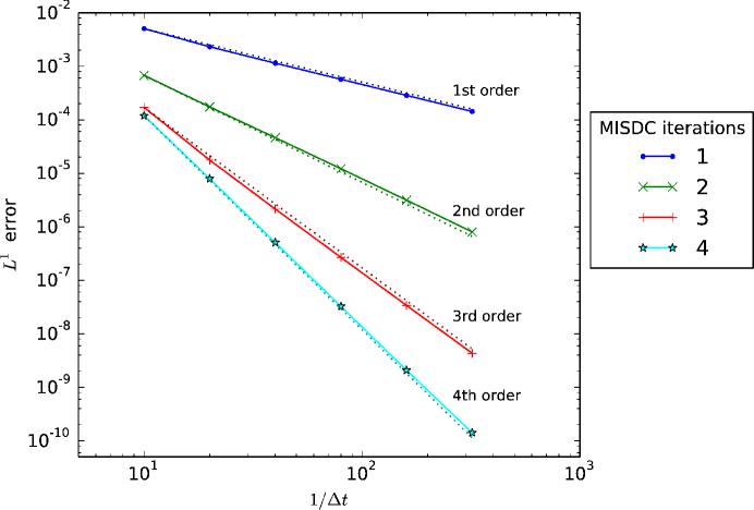
Figure 2. Log-log plot of $L^{1}$ error versus $1/\Delta t$ for the test PDE (65) using three Gauss-Lobatto nodes. Solid lines are the numerical results, and dotted lines indicate the expected convergence results.

5.2. Flame Simulations

We now analyse the convergence behaviour of our scheme on a set of more complex problems: premixed laminar flames burning hydrogen, methane, and dimethyl ether fuels that propagate through the domain. In all cases here, the diffusive and reactive processes are well-known to be numerically ’stiff’ on the advection time scales used to set our numerical time step. Because of this, we find that eight MISDC iterations are required per time step for robust integration, and we demonstrate in the following section that our strategy with this setting results in the expected convergence properties.

5.2.1. Hydrogen Flame

We study the performance of the MISDC algorithm to propagate a one-dimensional premixed hydrogen flame. The simulations are based on the GRIMech-3.0 [21] model and associated databases for thermodynamic relationships and mixture-averaged transport properties, as given in the CHEMKIN-III library [22] format. Note that we manually stripped the carbon-containing species and associated reactions from the model, since they are irrelevant for the hydrogen-air case. The resulting model for hydrogen-air mixtures consists of 9 species and 27 reactions.

The detailed structure of these flames feature the prominent role of molecular and atomic hydrogen, both of which diffuse considerably faster than the other species in the system. This differential diffusion between species has significant impact on steady 1D profiles; H and H₂ profiles tend to be considerably broader than the others, and this plays a key role in the flame stabilisation.

In this configuration, an unstrained one-dimensional flame propagates into a homogeneous hydrogen-air mixture. A steady solution consists of thermal and species profiles co-moving in a frame with the flame propagation. In the frame of the unburned fuel, the steady solution propagates toward the inlet at the unstrained laminar burning speed, $s_{L}$, which is a function of the inlet state. At the chosen conditions, $Y({\rm H}_{2}:{\rm O}_{2}:{\rm N}_{2})=(0.0107:0.2304:0.7589)$, $p$=1 atm, and $T$=298 K, $s_{L}=14.9$ cm s^-1. For each of our fourth-order flame simulations, we arbitrarily set the inlet velocity to 5 cm/s. Thus, the hydrogen flame propagates toward the inlet at 9.9 cm s^-1.

Initial flame profiles are generated for this study in two auxiliary steps. First, a steady one-dimensional solution is computed using the PREMIX code [23]. PREMIX incorporates a first-order difference scheme on nonuniform grid in one dimension. The PREMIX solution is translated into the frame of the unburned fuel, and interpolated onto a uniform grid with 8192 cells across a 1.2 cm domain. While this solution exhibits the essential features of the flame, it is not C2-continuous; higher-order discontinuities will pollute subsequent convergence analysis. To resolve this issue, we use the second-order low Mach number code from our previous work [2], to evolve the PREMIX solution for an additional $160~{}\mu$s using a time step of $\Delta t=0.8~{}\mu$s. Finally, the initial data to test our fourth-order algorithm is generated by averaging this solution to a set of uniform meshes, using $n=$ 128, 256, 512, and 1024 cells.

The initial data at each resolution are evolved for 1.6 ms so that the flame propagates approximately 16 $\mu$m across the mesh at a $\Delta t$ corresponding to an advective CFL of $\sigma\approx$ 0.28. The resulting profiles are compared to a reference solution as discussed above. The error and convergence results are presented in Table 1. Fourth-order convergence is observed in all variables. Note that HO₂ and H₂O₂ have the narrowest profiles of all species, and are therefore the most demanding to converge.

Table 1. Error and convergence rates for a premixed hydrogen flame using the fourth-order MISDC method with an advective CFL of $\sigma\approx 0.28$.

Variable	$L^{1}_{128}$	$r^{128/256}$	$L^{1}_{256}$	$r^{256/512}$	$L^{1}_{512}$
$Y({\rm H}_{2})$	5.91E-08	4.01	3.67E-09	3.98	2.33E-10
$Y({\rm O}_{2})$	1.10E-06	4.00	6.83E-08	4.05	4.14E-09
$Y({\rm H}_{2}{\rm O})$	1.01E-06	4.01	6.25E-08	4.05	3.76E-09
$Y({\rm H})$	1.17E-09	3.70	9.00E-11	3.91	5.97E-12
$Y({\rm O})$	2.70E-08	3.93	1.77E-09	4.01	1.10E-10
$Y({\rm OH})$	3.17E-08	4.01	1.97E-09	4.06	1.18E-10
$Y({\rm HO}_{2})$	3.56E-08	3.71	2.72E-09	3.88	1.86E-10
$Y({\rm H}_{2}{\rm O}_{2})$	1.41E-08	3.70	1.09E-09	3.84	7.58E-11
$Y({\rm N}_{2})$	1.77E-07	3.95	1.15E-08	4.07	6.85E-10
$\rho$	5.00E-09	4.01	3.10E-10	4.09	1.82E-11
$T$	1.21E-02	4.02	7.44E-04	4.05	4.48E-05
$\rho h$	6.77E+00	3.99	4.26E-01	4.07	2.54E-02

We now compare the accuracy of our new code to our previous second-order algorithm [2] and the previous Strang splitting algorithm [9]. In Figure 3, we plot the $L^{1}$ error for the intermediate species ${\rm HO}_{2}$ using each algorithm. We use the problem setup described in Section 5.2 of [2], which is the same as described above except that the time step is 20% larger than described above at each resolution. Note that not only is our new algorithm fourth-order, but at coarse resolution ($n=128$ with a domain length of 1.2 cm) the error in our fourth-order code is already a factor of 5 smaller than it was with our previous second-order code. In these simulations, the Strang split algorithm is not in the asymptotic convergence regime, and exhibits only first-order behaviour, as noted in [2].

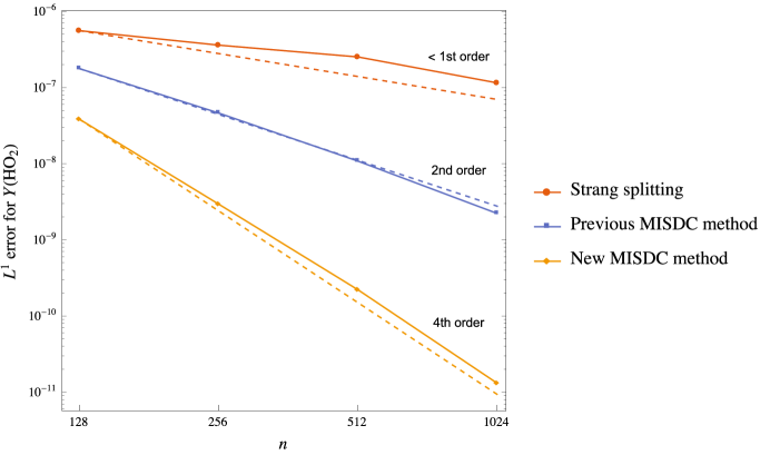
Figure 3. Log-log plot of $L^{1}$ error as a function of resolution ($n$ is the number of cells) for the intermediate species ${\rm HO}_{2}$ in a hydrogen flame using the Strang splitting code [9], second-order MISDC algorithm [2], and the fourth-order MISDC algorithm presented in this paper. Solid lines are the numerical results, and dotted lines give first, second, and fourth-order reference slopes.

We note that performing fewer than eight MISDC iterations in the fourth-order algorithm causes an observed order-reduction in our simulations unless we decrease the time step size as well. For the cases analysed when using four MISDC iterations, fourth-order is realised only when the time step is reduced by an order of magnitude or more. This is not particularly surprising given the disparity in time scales between the physical processes. In these cases, we found it more efficient computationally to increase the time step size, even though more MISDC iterations are required per step.

Next, we examine the effectiveness of the volume discrepancy algorithm in reducing the thermodynamic drift. We performed the exact same set of simulations described above, but disabled the $\delta\chi$ volume discrepancy correction term. In Figure 4, we plot the thermodynamic pressure, $p_{\rm EOS}$, as a function of space for the $n=128$ simulation with and without the $\delta\chi$ correction terms. The correction causes the pressure to stay on the equation of state to within $\sim 3$ g/(cm-s²), whereas without the correction, the pressure drifts by $\sim 40,000$ g/(cm-s²). The blue temperature plot is included for reference, indicating the location and shape of the flame. Next, in Figure 5 we show a plot of the thermodynamic drift, $p_{\rm EOS}-p_{0}$, as a function of space for the $n=128,256,512,$ and $1024$ simulations with the $\delta\chi$ correction term. The $\delta\chi$ correction term clearly drives the pressure drift to zero as spatial resolution increases, as the magnitude of the drift decreases by roughly a factor of 8 as we increase resolution by a factor of 2. For the $n=1024$ simulation, the maximum value of $|p_{\rm EOS}-p_{0}|$ is less than 0.01 g/(cm-s²).

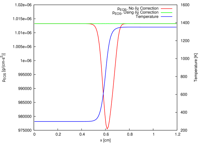
Figure 4. A plot of the thermodynamic pressure, $p_{\rm EOS}$, as a function of space for the $n=128$ simulation at the final time with and without the $\delta\chi$ volume discrepancy correction. The blue temperature plot is included for reference, indicating the location and shape of the flame.

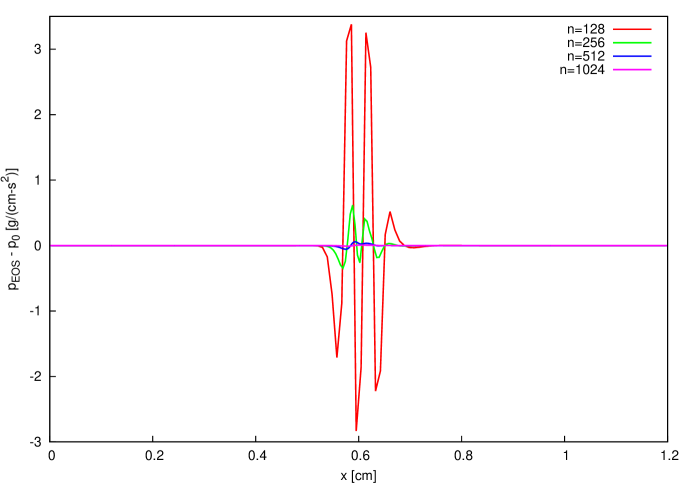
Figure 5. A plot of the thermodynamic drift, $p_{\rm EOS}-p_{0}$, as a function of space for the $n=128,256,512,$ and $1024$ simulations with the $\delta\chi$ correction term.

5.2.2. Methane Flame

We next study the performance of the MISDC algorithm using a one-dimensional premixed methane flame. The simulations are based on the GRIMech-3.0 [21] model and associated database, as given in the CHEMKIN-III library [22] format. The GRIMech-3.0 model consists of 53 species with a 325-step chemical reaction network for premixed methane combustion. This example is particularly challenging because of the extremely broad range of chemical time scales, which range from $10^{-4}$ to $10^{-10}$ seconds.

Similar to the hydrogen flame, the initial conditions are obtained by interpolating from a frame-shifted, refined steady, one-dimensional solution computed using the PREMIX code. For this case, the inlet stream at $T$=298 K and $p$=1 atm has composition, $Y({\rm O}_{2}:{\rm CH}_{4}:{\rm N}_{2})=(0.2238:0.0392:0.7370)$ so that the unstrained laminar burning speed is $s_{L}=18.9$ cm s^-1. The PREMIX solution is interpolated onto a 1.2 cm domain with 8192 uniform cells, and evolved with the second-order code from [2] for $80~{}\mu$s with $\Delta t=0.4~{}\mu$s. The resulting solution is averaged down to coarse uniform meshes of $n=$ 128, 256, 512, and 1024 cells to provide the initial conditions for testing the fourth-order algorithm. We evolve the system for $800~{}\mu$s to allow the solution to propagate $\sim$111 $\mu$m across the mesh with $\sigma$$\approx$ 0.21. The error and convergence results for the primary reactants, products, and key intermediate species, as well as the remaining thermodynamic variables are presented in Table 2. We see fourth-order convergence in all variables, noting that for $Y({\rm CH}_{3})$, the profile is extremely thin so that higher resolution is required to reach the asymptotic regime.

Table 2. Error and convergence rates for a premixed methane flame using the fourth-order MISDC method with an advective CFL of $\sigma\approx 0.21$.

Variable	$L^{1}_{128}$	$r^{128/256}$	$L^{1}_{256}$	$r^{256/512}$	$L^{1}_{512}$
$Y({\rm CH}_{4})$	1.11E-06	4.00	6.97E-08	3.98	4.42E-09
$Y({\rm O}_{2})$	3.77E-06	3.96	2.42E-07	4.07	1.44E-08
$Y({\rm H}_{2}{\rm O})$	2.30E-06	4.02	1.42E-07	4.05	8.53E-09
$Y({\rm CO}_{2})$	1.87E-06	4.02	1.15E-07	4.07	6.87E-09
$Y({\rm CH}_{3})$	3.11E-08	2.48	5.59E-09	3.75	4.16E-10
$Y({\rm CH}_{2}{\rm(S)})$	8.01E-11	4.14	4.54E-12	3.85	3.15E-13
$Y({\rm O})$	1.05E-07	4.08	6.20E-09	3.90	4.16E-10
$Y({\rm H})$	3.48E-09	3.83	2.45E-10	3.81	1.75E-11
$Y({\rm N}_{2})$	3.58E-07	3.74	2.68E-08	4.00	1.67E-09
$\rho$	1.25E-08	4.03	7.64E-10	4.05	4.61E-11
$T$	3.52E-02	4.01	2.18E-03	4.06	1.31E-04
$\rho h$	4.09E+01	3.97	2.60E+00	4.00	1.62E-01

5.2.3. Dimethyl Ether Flame

Finally, we present a one-dimensional simulation of a premixed flame using a 39-species, 175-reaction dimethyl ether (DME) chemistry mechanism [24]. The DME mechanism used in this test is extremely stiff. It is quite challenging to capture the nonlinear coupling between diffusion and reaction chemistry, while evolving the system on the much slower advection scales. The inlet stream at $T$=298 K has composition, $Y({\rm CH}_{3}{\rm OCH}_{3}:{\rm O}_{2}:{\rm N}_{2})=(0.0726:0.2160:0.7114)$, and $p$=1 atm; the unstrained laminar burning speed is $s_{L}=24.9$ cm s^-1. The initial PREMIX-computed profiles are interpolated onto a 0.6 cm domain with 8192 uniform cells and evolved for $16~{}\mu$s using the second-order algorithm from [2] at $\Delta t=0.08~{}\mu$s. The resulting solution is averaged onto uniform grids of $n=$ 128, 256, 512, and 1024 cells to provide initial data for testing our fourth-order algorithm. We evolve the system for 320 $\mu$s to allow the solution to propagate 64 $\mu$m across the domain at $\sigma\approx$ 0.25. The error and convergence results for the primary reactants, products, and key intermediate species [24], as well as the remaining thermodynamic variables are presented in Table 3. We see fourth-order convergence in all variables.

Table 3. Error and convergence rates for a dimethyl ether flame using the fourth-order MISDC method with an advective CFL of $\sigma\approx 0.25$.

Variable	$L^{1}_{128}$	$r^{128/256}$	$L^{1}_{256}$	$r^{256/512}$	$L^{1}_{512}$
$Y({\rm CH}_{3}{\rm OCH}_{3})$	2.29E-06	3.83	1.62E-07	3.93	1.06E-08
$Y({\rm O}_{2})$	2.99E-06	3.63	2.42E-07	4.02	1.49E-08
$Y({\rm CO}_{2})$	2.51E-06	3.83	1.76E-07	4.04	1.07E-08
$Y({\rm H}_{2}{\rm O})$	1.62E-06	3.51	1.42E-07	4.01	8.85E-09
$Y({\rm CH}_{3}{\rm OCH}_{2}{\rm O}_{2})$	1.55E-10	4.51	6.76E-12	3.88	4.61E-13
$Y({\rm OH})$	3.24E-07	3.80	2.32E-08	4.02	1.43E-09
$Y({\rm HO}_{2})$	1.46E-07	3.80	1.05E-08	3.95	6.77E-10
$Y({\rm O})$	1.70E-07	3.55	1.46E-08	3.92	9.66E-10
$Y({\rm H})$	8.35E-09	3.68	6.52E-10	3.96	4.20E-11
$Y({\rm N}_{2})$	1.09E-06	3.76	8.01E-08	3.93	5.25E-09
$\rho$	9.44E-09	3.67	7.42E-10	4.02	4.58E-11
$T$	2.54E-02	3.59	2.11E-03	4.01	1.31E-04
$\rho h$	5.89E+01	3.83	4.15E+00	4.02	2.56E-01

6. Conclusions and Future Work

We have developed a fourth-order finite-volume algorithm for low Mach number reacting flow with detailed kinetics and transport. The approach iteratively couples advection, diffusion, and reaction processes using efficient numerical methods for each step. The method exhibits much greater accuracy, even at coarse resolution, than our previous second-order deferred correction strategy [2] and Strang splitting algorithms [9]. We have incorporated a volume discrepancy scheme that allows us to simultaneously conserve mass and enthalpy while satisfying the equation of state to a high degree of accuracy. The volume discrepancy scheme is iterative, and naturally fits within our MISDC framework with negligible computational cost. We have discussed an instability with our previous development path that did not allow the method to extend to higher-order and demonstrated that our approach is stable and convergent for a much broader range of parameters.

As discussed in the Results section, a key parameter in our new scheme is the number of SDC iterations taken on each time step. Formally, the algorithm requires four iterations to couple together all processes and achieve fourth-order convergence behavior. However, because our difficult demonstration problems feature cases with relatively stiff diffusion and reaction processes, the inter-process coupling at the advection time scale was not sufficiently accurate to achieve the design rates. There were at least two remedies to improve the coupling: reduce the time step or increase the number of iterations per step – both of which make the algorithm more costly in different ways. By trial and error, we found that 8 iterations per step was sufficient to achieve fourth-order accuracy for all cases presented. It is likely that an adaptive procedure can be developed to optimize this choice for the general case.

The long-term goal of this effort is to extend the method described here to multidimensional, adaptive mesh refinement (AMR) simulations. One issue concerning this goal is extending the projection method formulation to multiple dimensions, where the velocity field is no longer uniquely specified by the boundary conditions and the thermodynamic state. Previous high-order SDC algorithms for incompressible flows (e.g. [18, 1]) have been based on a gauge variable formulation which does not immediately extend to more general low Mach number models. One possible path forward is to utilise finite volume Stokes solvers to allow us to solve the coupled viscous/projection step to arbitrary spatial accuracy, and incorporate this into a method of lines approach to allow for higher-order temporal integration. Some work has already been done in efficient projection-preconditioned finite volume Stokes solvers [25], which fit well in our SDC based algorithms. We would also like to implement an SDC based AMR algorithm that subcycles in time as in multilevel SDC methods [26]. Finally, including stratification in our low Mach number reacting flow models will allow them to be used in atmospheric [27] and astrophysical [28] simulations.

Appendix A Convergence analysis of the previous method

Here we examine the convergence properties of MISDC iterations of the method described in [2]. As in Section 3.1, we consider the linear ODE

(68) $$\phi_{t}=a\phi+d\phi+r\phi\equiv F(\phi),$$

For simplicity we will consider only two temporal nodes, $t^{n,0}=t^{n}$ and $t^{n,1}=t^{n+1}=t^{n}+\Delta t$. The corresponding Gauss-Lobatto quadrature rule in this case is the trapezoidal rule. We compute a provisional solution using the diffusion correction equation using the implicit formula

(69) $$\phi^{1,(k+1)}_{\rm AD}=\phi^{n}+\Delta t^{m}\left[d\phi_{\rm AD}^{1,(k+1)}-d\phi^{1,(k)}\right]+I\left[(a+d)\phi^{(k)}\right]+I_{R}^{(k)}.$$

The term $I_{R}^{(k)}$ is equal to the integral of the reaction term. The reaction correction equation is differentiated to obtain the ODE

(70) $$\phi^{(k+1)}_{t}(t)=r\phi^{(k+1)}(t)+d\phi_{\rm AD}^{1,(k+1)}-d\phi^{1,(k)}+A(\phi^{(k)},t)+D(\phi^{(k)},t).$$

Here $A$ and $D$ are polynomials representing the advection and diffusion contributions. We require that the integrals of $A$ and $D$ are equal to the numerical quadrature. In [2], $A$ and $D$ are chosen to be the averages at times $t^{n}$ and $t^{n}+\Delta t$. In order for this method to generalise to higher order, we would need to represent $A$ and $D$ by higher degree polynomials. For instance, we can take $A$ and $D$ to be the linear interpolants given by

(71) $$A(\phi^{(k)},t) =(1-t/\Delta t)a\phi^{0,(k)}+(t/\Delta t)a\phi^{1,(k)},$$

(72) $$D(\phi^{(k)},t) =(1-t/\Delta t)d\phi^{0,(k)}+(t/\Delta t)d\phi^{1,(k)},$$

so that their integrals are equal to the quadrature computed using the trapezoid rule. The reaction integral can then be computed by integrating both sides of (70), and rearranging:

$$I_{R}^{(k+1)} \equiv \int_{t^{n}}^{t^{n}+\Delta t}r\phi^{(k+1)}(\tau)\ d\tau$$

$$= \phi^{1,(k+1)}-\phi^{0,(k+1)}+\Delta t\left[\frac{a\phi^{0,(k)}+a\phi^{1,(k)}}{2}+\frac{d\phi^{0,(k)}-d\phi^{1,(k)}}{2}+d\phi_{\rm AD}^{1,(k+1)}\right].$$

We notice that equation (70) is an ODE of the form

$$y_{t}(t) =ry+c_{1}t+c_{0},$$

$$y(0) =0,$$

to which the exact solution is given by

(74) $$y(t)=-\frac{1}{r^{2}}\left(c_{1}rt-c_{1}e^{rt}+c_{0}r-c_{0}e^{rt}+c1\right).$$

Expanding expressions (69) and (70), using the solution given by (74), we see that the difference between successive iterates is given by

$$\phi^{1,(k+1)}-\phi^{1,(k)}=\alpha\left[\phi^{1,(k)}-\phi^{1,(k-1)}\right]+\beta\left[I_{R}^{(k)}-I_{R}^{(k-1)}\right],$$

where, in the case of the linear ODE (68), $\alpha$ and $\beta$ are given by

$$\alpha =-\tfrac{a\left(2d\Delta t+\Delta tr(d\Delta t-2)+e^{\Delta tr}(d\Delta t(\Delta tr-2)+2)-2\right)+d\left(e^{\Delta tr}\left(d\Delta t^{2}r-2\Delta t(d+r)+2\right)+d\Delta t(\Delta tr+2)-2\right)}{2\Delta tr^{2}(d\Delta t-1)}$$

$$\beta =\tfrac{d(e^{r\Delta t}-1)}{r(d\Delta t-1)}.$$

We note that a sufficient condition for the iterative scheme to converge is $|\alpha|,|\beta|<1$. For fixed $a$, we observe that the set of parameters $(d,r)$ that satisfy this condition (Figure 1) is exceedingly small.

Furthermore, making the ansatz that $a=\tilde{a}/\Delta x$, $d=\tilde{d}/\Delta x^{2}$, and $\Delta t=\lambda\Delta x$, we can compute the limits of $\alpha$ and $\beta$ as $\Delta x$ tends to zero. We see

$$\lim_{\Delta x\to 0}\alpha=\frac{6-\tilde{d}\tilde{r}\lambda^{2}}{12},\qquad\lim_{\Delta x\to 0}\beta=1.$$

We therefore conclude that the sufficient condition for the iterative scheme to converge is met only for a limited choice of coefficients $\tilde{a}$, $\tilde{d}$ and $\lambda$. This is in contrast to the present method, for which convergence is guaranteed as $\Delta x$ tends to zero, for any choice of coefficients, as demonstrated in Section 3.1. Indeed, numerical experiments indicate that this method suffers from extremely restrictive time-step conditions in order to obtain convergence.

References

- [1] A.S. Almgren, A.J. Aspden, J.B. Bell, and M. Minion, On the use of higher-order projection methods for incompressible turbulent flow, SIAM J. Sci. Comput. 53 (2013).
- [2] A. Nonaka, J.B. Bell, M.S. Day, C. Gilet, A.S. Almgren, and M.L. Minion, A deferred correction coupling strategy for low Mach number flow with complex chemistry, Combust. Theory Modelling (2012) available at http://www.tandfonline.com/doi/full/10.1080/13647830.2012.701019.
- [3] A. Dutt, L. Greengard, and V. Rokhlin, Spectral Deferred Correction Methods for Ordinary Differential Equations, BIT 40 (2000), pp. 241–266.
- [4] M.L. Minion, Semi-Implicit Spectral Deferred Correction Methods for Ordinary Differential Equations, Comm. Math. Sci. 1 (2003), pp. 471–500.
- [5] A. Bourlioux, A.T. Layton, and M.L. Minion, High-Order Multi-Implicit Spectral Deferred Correction Methods for Problems of Reactive Flow, Journal of Computational Physics 189 (2003), pp. 651–675.
- [6] A.T. Layton and M.L. Minion, Conservative Multi-Implicit Spectral Deferred Correction Methods for Reacting Gas Dynamics, Journal of Computational Physics 194 (2004), pp. 697–715.
- [7] P. Zadunaisky, A method for the estimation of errors propagated in the numerical solution of a system of ordinary differential equations, in The Theory of Orbits in the Solar System and in Stellar Systems. Proceedings of International Astronomical Union, Symposium 25G. Contopoulos ed., , Thessaloniki, 1964, pp. 281–287.
- [8] R.B. Pember, L.H. Howell, J.B. Bell, P. Colella, W.Y. Crutchfield, W.A. Fiveland, and J.P. Jessee, An Adaptive Projection Method for Unsteady Low-Mach Number Combustion, Comb. Sci. Tech. 140 (1998), pp. 123–168.
- [9] M.S. Day and J.B. Bell, Numerical simulation of laminar reacting flows with complex chemistry, Combust. Theory Modelling 4 (2000), pp. 535–556.
- [10] R.G. Rehm and H.R. Baum, The equations of motion for thermally driven buoyant flows, Journal of Research of the National Bureau of Standards 83 (1978), pp. 297–308.
- [11] A. Majda and J.A. Sethian, Derivation and Numerical Solution of the Equations of Low Mach Number Combustion, Comb. Sci. Tech. 42 (1985), pp. 185–205.
- [12] R.J. Kee, J. Warnatz, and J. Miller, Fortran computer-code package for the evaluation of gas-phase viscosities, conductivities, and diffusion coefficients., NTIS, SPRINGFIELD, VA(USA), 1983, 37 (1983).
- [13] J. Warnatz, Influence of transport models and boundary conditions on flame structure, , in Numerical methods in laminar flame propagation Springer, 1982, pp. 87–111.
- [14] A.T. Layton and M.L. Minion, Implications of the Choice of Quadrature Nodes for Picard Integral Deferred Corrections Methods for Ordinary Differential Equations, BIT 45 (2005), pp. 341–373.
- [15] H.N. Najm, P.S. Wyckoff, and O.M. Knio, A semi-implicit numerical scheme for reacting flow. I. Stiff chemistry, J. Comp. Phys. 143 (1998), pp. 381–402.
- [16] O.M. Knio, H.N. Najm, and P.S. Wyckoff, A semi-implicit numerical scheme for reacting flow. I. Stiff, operator-split formulation, J. Comp. Phys. 154 (1999), pp. 428–467.
- [17] F. Perini, E. Galligani, and R.D. Reitz, An Analytical Jacobian Approach to Sparse Reaction Kinetics for Computationally Efficient Combustion Modeling with Large Reaction Mechanisms, Energy & Fuels 26 (2012), pp. 4804–4822.
- [18] S.Y. Kadioglu, R. Klein, and M.L. Minion, A Fourth-Order Auxiliary Variable Projection Method for Zero-Mach number gas dynamics, Journal of Computational Physics 227 (2008), pp. 2012–2043.
- [19] P. McCorquodale and P. Colella, A high-order finite-volume method for conservation laws on locally refined grids, Communications in Applied Mathematics and Computational Science 6 (2011), pp. 1–25.
- [20] Q. Zhang, H. Johansen, and P. Colella, A fourth-order accurate finite-volume method with structured adaptive mesh refinement for solving the advection-diffusion equation, SIAM Journal on Scientific Computing 34 (2012), pp. B179–B201.
- [21] M. Frenklach, H. Wang, M. Goldenberg, G.P. Smith, D.M. Golden, C.T. Bowman, R.K. Hanson, W.C. Gardiner, and V. Lissianski, GRI-Mech—An Optimized Detailed Chemical Reaction Mechanism for Methane Combustion, GRI-95/0058, Gas Research Institute, 1995 http://www.me.berkeley.edu/gri_mech/.
- [22] R.J. Kee, R.M. Ruply, E. Meeks, and J.A. Miller, CHEMKIN-III: A FORTRAN Chemical Kinetics Package for the Analysis of Gas-phase Chemical and Plasma Kinetics, Technical Report SAND96-8216, Sandia National Laboratories, Livermore, 1996.
- [23] R.J. Kee, J.F. Grcar, M.D. Smooke, and J.A. Miller, PREMIX: A Fortran Program for Modeling Steady, Laminar, One-Dimensional Premixed Flames, Technical Report SAND85-8240, Sandia National Laboratories, Livermore, 1983.
- [24] G. Bansal, A. Mascarenhas, and J.H. Chen, Direct numerical simulations of autoignition in stratified dimethyl-ether (DME)/air turbulent mixtures, Combustion and Flame 162 (2015), pp. 688 – 702.
- [25] M. Cai, A. Nonaka, J.B. Bell, B.E. Griffith, and A. Donev, Efficient Variable-Coefficient Finite-Volume Stokes Solvers, Commun. Comput. Phys. 16 (2014), pp. 1263–1297.
- [26] R. Speck, D. Ruprecht, M. Emmett, M. Minion, M. Bolten, and R. Krause, A multi-level spectral deferred correction method, BIT Numerical Mathematics 55 (2015), pp. 843–867.
- [27] M. Duarte, A.S. Almgren, and J.B. Bell, A low Mach number model for moist atmospheric flows, J. Atmos. Sci. 72 (2014), pp. 1605–1647.
- [28] A. Nonaka, A. Almgren, J. Bell, M. Lijewski, C. Malone, and M. Zingale, MAESTRO: An adaptive low Mach number hydrodynamics algorithm for stellar flows, The Astrophysical Journal Supplement Series 188 (2010), p. 358.