Semi-Holography for Heavy Ion Collisions: Self-Consistency and First Numerical Tests

Abstract

We present an extended version of a recently proposed semi-holographic model for heavy-ion collisions, which includes self-consistent couplings between the Yang-Mills fields of the Color Glass Condensate framework and an infrared AdS/CFT sector, such as to guarantee the existence of a conserved energy-momentum tensor for the combined system that is local in space and time, which we also construct explicitly. Moreover, we include a coupling of the topological charge density in the glasma to the same of the holographic infrared CFT. The semi-holographic approach makes it possible to combine CGC initial conditions and weak-coupling glasma field equations with a simultaneous evolution of a strongly coupled infrared sector describing the soft gluons radiated by hard partons. As a first numerical test of the semi-holographic model we study the dynamics of fluctuating homogeneous color-spin-locked Yang-Mills fields when coupled to a homogeneous and isotropic energy-momentum tensor of the holographic IR-CFT, and we find rapid convergence of the iterative numerical procedure suggested earlier.

1 Introduction

Describing the full time evolution and equilibration process of the fireball created in ultrarelativistic heavy-ion collisions is an extremely difficult task due to the interplay of perturbative and non-perturbative phenomena. Tracing the full evolution appears to require a patchwork of different effective theories, each designed to describe a certain stage of the evolution and only applicable to specific physical observables.

According to the color glass condensate (CGC) framework Gelis:2010nm , at very early times $\tau\sim 1/Q_{s}$ the system is dominated by gluons with typical momenta of the order of the semi-hard saturation scale $Q_{s}$, which are relatively weakly coupled (when $Q_{s}$ is large), $\alpha_{s}(Q_{s})\ll 1$, but which have high occupation numbers $\sim 1/\alpha_{s}$. This admits a description in terms of semiclassical Yang-Mills fields, also called the glasma Lappi:2006fp , which has been studied by numerical solutions of classical Yang-Mills equations Romatschke:2006nk ; Gelis:2013rba ; Berges:2013fga . As the system undergoes rapid longitudinal expansion and the occupation number of the semi-hard gluons drops, soft gluons are emitted abundantly, whose dynamics is characterised by a significantly larger coupling $\alpha_{s}(\mu<Q_{s})$. This growing soft sector is presumed to play a crucial role in the evolution of the whole system.

While the rapid thermalization suggested by experimental data might be captured by an effective kinetic theory description extrapolated to strong coupling Kurkela:2015qoa , insight into isotropization and thermalization of a strongly coupled quantum field theory can be comparatively directly gained by gauge/gravity duality. The latter maps the thermalization process to black hole formation in asymptotically anti-de Sitter space DeWolfe:2013cua ; Chesler:2013lia . By comparing results from hydrodynamic simulations with the full holographic evolution it was found that the system is accurately described by hydrodynamics although large viscous corrections are still present. Later the system isotropizes and reaches local thermal equilibrium Chesler:2010bi ; Heller:2011ju . (For an extensive list of references see the recent review Chesler:2015lsa .)

The mechanism how the initial state makes a transition to a state that is amenable to a hydrodynamic description is however different for weak and strong coupling (although quantitatively there might exist a smooth interpolation Keegan:2015avk ). At asymptotically high energies and parametrically small coupling the thermalization pattern is of the bottom-up type Baier:2000sb ; Kurkela:2011ub , where first the soft gluons form a thermal bath which then draws energy from the hard modes. On the other hand, at infinite coupling the thermalization process as obtained via the gauge/gravity correspondence is top-down, meaning that highly energetic modes reach their thermal distribution first Balasubramanian:2011ur . By considering corrections to the infinite-coupling limit it was shown in Steineder:2012si ; Stricker:2013lma that there indeed exists a transition between the two behaviors at intermediate coupling.

A description of the whole evolution from within a single framework and from first principles is elusive at this point. So far most studies have either utilized solely a weakly coupled approach or a strongly coupled one, but in order to understand the evolution of the colliding matter better, one needs to combine the different effective descriptions for the different stages as well as weak and strong coupling phenomena. In recent years various attempts in this direction have been made. For example, in vanderSchee:2013pia different effective descriptions were patched together. The far-from-equilibrium initial stage was simulated by colliding shock waves using numerical AdS/CFT, whose results were used as an input for the hydrodynamic evolution, which subsequently served as an input for the kinetic theory describing the low density hadronic stage.

However, the initial conditions set up for AdS/CFT calculations, even in state-of-the-art shock-wave collisions, have no clear connection to those derived directly from (weak-coupling) QCD in the (nonperturbative) CGC framework. It would seem highly desirable to be able to connect the two approaches and follow the combined evolution of weakly coupled semi-hard gluons and a strongly interacting soft sector.

The first semi-holographic proposals for describing interactions between a weakly coupled and a strongly coupled sector, where the strongly coupled sector is described by a holographic dual, were made in the context of non-Fermi liquids Faulkner:2010tq ; Mukhopadhyay:2013dqa . In the context of heavy-ion collisions one attempt to combine weak and strong coupling was made in a so-called hybrid approach to describe the energy loss of jets moving through a strongly coupled medium Casalderrey-Solana:2014bpa , where the soft in-medium effects were modeled by using insights from gauge/gravity duality. However, in this case no back reaction of the soft medium to the hard partons was taken into account.

A different route was recently taken in Iancu:2014ava where a semi-holographic model for thermalization in heavy-ion collisions was presented. This model is able to incorporate the interaction between weakly coupled hard and strongly coupled soft modes but so far lacks verification by carrying out a concrete calculation. The goal of this work is to refine and test the proposal of Iancu:2014ava with regard to its internal self-consistency and numerical practicability (while not yet attempting to shed new light on thermalization in heavy-ion collisions).

The outline of this paper is as follows. In Sec. 2 we review and also extend the semi-holographic model of Iancu:2014ava . Specifically, we present a reformulation of the model which permits the definition of a locally conserved energy-momentum tensor of the combined system of hard and soft degrees of freedom. In Sec. 3 we present a simple test case for semi-holographic glasma evolution. We truncate the couplings of the model developed in Sec. 2, such that only gravitational degrees of freedom are excited in the holographic sector and moreover impose homogeneity and isotropy in both the hard and the soft sector. As a consequence the (time-dependent) gravity dual of this test case can be treated analytically, but due to the Birkhoff theorem does not allow for dynamical black-hole formation or perturbation. Thus, the soft degrees of freedom captured by the dual strongly coupled field theory cannot equilibrate with the hard degrees of freedom, i.e., this simple test case is too restricted for permitting to study thermalization. It however allows us to carry out a first proof-of-principle calculation, where we can verify the convergence of an iterative numerical solution of the semi-holographic set-up. Section 4 contains our conclusions and an outlook.

2 Action and energy-momentum tensor of the semi-holographic set-up

Following Iancu:2014ava , in this section we construct an action where the description of a semi-hard gluon (UV) sector and that of a strongly-interacting soft gluon (IR) sector can be coupled self-consistently. In this paper, we will treat the semi-holographic model phenomenologically including minimalistic hard-soft couplings only, without attempting a derivation from first principles; a rigorous framework for a possible derivation has been recently proposed in Behr:2015aat .

The assumptions that provide the basis of the semi-holographic model for heavy-ion collisions in Iancu:2014ava are as follows:

1. the over-occupied semi-hard (UV) gluons allow for a description in terms of a classical Yang–Mills theory as in the glasma model Gelis:2010nm ; Lappi:2006fp ,

2. the infrared sector is described by a conformal field theory (IR-CFT) which is approximated by the strong-coupling large-$N$ limit such that a classical dual holographic description is possible,

3. the IR-CFT is marginally deformed such that its marginal couplings become functionals of the color fields of the glasma, while the marginal operators of the infrared conformal field theory (IR-CFT) appear as self-consistent fields which modify the classical Yang-Mills dynamics of the color fields of the glasma, and

4. the hard-soft couplings describing the mutual feedback between the IR-CFT and the color fields of the glasma involve local gauge-invariant operators of both sectors, and the coupling constants are given by a dimensionless number times $Q_{s}^{-4}$, with $Q_{s}$ being the saturation scale of the colliding nuclei.

In addition to the proposal in Iancu:2014ava we demand a well defined action principle that allows for the construction of a conserved energy-momentum tensor for the combined system living in flat space.

For the action describing the interactions between the hard and soft modes, which satisfies all the criteria mentioned above, we propose

$$S=S_{\mathrm{YM}}+W_{\mathrm{CFT}}[g^{({\rm b})}_{\mu\nu},\phi^{({\rm b})},\chi^{({\rm b})}]\,,$$ (1)

which we will discuss now in detail.

We start with the Yang-Mills part of the action and for the time being, consider a classical Yang-Mills theory living on an arbitrary non-dynamical background metric $g^{\mathrm{YM}}_{\mu\nu}$, which in the end will be set to the flat Minkowski metric. This is for technical purposes only because it is convenient for identifying the tensorial properties of the variables to be defined below. The Yang-Mills action $S_{\mathrm{YM}}$ in this background is given by

$$S_{\mathrm{YM}}=-\int\mathrm{d}^{4}x\,\sqrt{-g^{\mathrm{YM}}}\;h,\;\qquad h:=\frac{1}{4N_{c}}\mathrm{Tr}\left(F_{\mu\nu}F^{\mu\nu}\right).$$ (2)

We use the normalisation $\mathrm{Tr}(T^{a}T^{b})=N_{c}\delta^{ab}$ for the generators of the $SU(N_{c})$ gauge group together with the standard convention for the covariant derivative $D_{\mu}=\nabla_{\mu}-igA_{\mu}^{a}T^{a}$, where $\nabla_{\mu}$ is the Levi-Civita connection with respect to $g^{\mathrm{YM}}_{\mu\nu}$.

The gauge invariant operators of the UV sector used to deform the IR-CFT are $h$, the energy-momentum tensor of the Yang-Mills fields, $t_{\mu\nu}$, which takes the standard form

$$t_{\mu\nu}=\frac{1}{N_{c}}\mathrm{Tr}\left(F_{\mu\alpha}F_{\nu}^{~{}\alpha}-\frac{1}{4}g^{\mathrm{YM}}_{\mu\nu}F_{\alpha\beta}F^{\alpha\beta}\right)\,,$$ (3)

and the Yang-Mills Pontryagin density

$$a:=\frac{1}{4\sqrt{-g^{\mathrm{YM}}}N_{c}}\mathrm{Tr}\left(F_{\mu\nu}\tilde{F}^{\mu\nu}\right).$$ (4)

Notice that $a$, $h$ as well as $t_{\mu\nu}$ are functionals of the background metric $g^{\mathrm{YM}}_{\mu\nu}$.

The second part of the action (1), $W_{\mathrm{CFT}}$, is the generating functional of the IR-CFT, provided by the on-shell gravitational action of its gravity dual. The gravitational dynamics will be described by Einstein’s gravity with asymptotically AdS boundary conditions minimally coupled to matter. However, at this point we can be completely agnostic about the IR-CFT generating functional $W_{\rm CFT}$, meaning that we do not need to know its explicit form in terms of the elementary fields. We only need that $W_{\rm CFT}$ describes a marginally deformed CFT in presence of three background sources, namely $g^{\rm(b)}_{\mu\nu}$, $\phi^{\rm(b)}$ and $\chi^{\rm(b)}$, which couple to the three marginal operators of dimension $4$, namely $\mathcal{T}_{\mu\nu}$ (the energy-momentum tensor of the CFT), $\mathcal{H}$ (the glueball/Lagrangian density operator of the CFT) and $\mathcal{A}$ (the topological charge density operator of the CFT), respectively. The bulk fields dual to these operators are the metric $G_{MN}$, the dilaton $\phi$, and the axion $\chi$. For example, the IR-CFT energy-momentum tensor can be obtained from the asymptotic expansion of the bulk metric $G_{MN}$ in Fefferman-Graham gauge, which takes the form

$$G_{\rho\rho} = \frac{l^{2}}{\rho^{2}},\quad\quad G_{\rho\mu}=0,$$

$$G_{\mu\nu} = \frac{l^{2}}{\rho^{2}}\left(g^{({\rm b})}_{\mu\nu}+\cdot\cdot\cdot+\rho^{4}\left(\frac{4\pi G_{5}}{l^{3}}\mathcal{T}_{\mu\nu}+X_{\mu\nu}\right)+\mathcal{O}\left(\rho^{6}\right)\right),$$ (5)

where $\rho$ denotes the holographic radial coordinate, with $\rho=0$ being the location of the conformal boundary of the bulk spacetime. The tensor $X_{\mu\nu}$ above is also a local functional of the boundary metric $g^{({\rm b})}_{\mu\nu}$, is non-trivial when the latter is curved, and is explicitly known (see deHaro:2000xn ). Likewise the boundary values of the axion and dilaton are $\phi^{\rm(b)}$ and $\chi^{\rm(b)}$, respectively.

We also have to specify how $g^{\rm(b)}_{\mu\nu}$, $\phi^{\rm(b)}$ and $\chi^{\rm(b)}$ are determined by the Yang-Mills color fields as appropriate gauge-invariant tensors. At leading order in $Q_{s}^{-4}$, the most general forms of these sources are:

$$g^{({\rm b})}_{\mu\nu} = g^{\mathrm{YM}}_{\mu\nu}+\frac{\gamma}{Q_{s}^{4}}t_{\mu\nu},$$ (6a)

$$\phi^{({\rm b})} = \frac{\beta}{Q_{s}^{4}}h\;,\qquad\chi^{({\rm b})}=\frac{\alpha}{Q_{s}^{4}}a,$$ (6b)

where $\gamma$, $\beta$ and $\alpha$ are dimensionless free parameters. The IR-CFT $\mathcal{T}_{\mu\nu}$ is thus determined by the color fields, after assuming appropriate initial conditions and requiring absence of naked singularities in the bulk spacetime. Similarly, all other IR-CFT operators are also determined by the color fields of the glasma via holographic dynamics.

Heuristically, the above form of the bulk fields at the boundary can be understood in terms of renormalisation group (RG) flow, where the scale of the flow is related to the radial direction of the dual gravity theory. Going along the radial coordinate both the sources (including the background metric) and the single trace operators of the CFT evolve in the dual geometries. It was shown in Behr:2015yna ; Behr:2015aat that it can be recast in a precise form of RG flow in which the Ward identities of single trace operators giving local conservation laws preserve their form along the scale evolution, so that the sources become functionals of the ultraviolet degrees of freedom. Although this RG flow occurs in a fixed background metric, the sources emerge as scale-dependent effective dynamical objects whose evolution is described by a dual diffeomorphism-invariant classical gravity theory in one higher dimension in the large $N$ limit. In order to include weakly coupled UV degrees of freedom which cannot be described by a dual classical gravity theory, it is natural to stop the geometric description of dynamics at a certain scale, in our case the saturation scale $Q_{s}$ and assume that the effective sources and background metric at that scale are functionals of the operators of the weakly coupled UV fields instead of the UV modes of the strongly coupled holographic CFT. Therefore the boundary metric (6a) should be rather viewed as an effective metric that accounts for the marginal deformation of the IR-CFT due to the coupling between the soft and hard modes at the scale $Q_{s}$. In fact, as we will show below, the full energy-momentum tensor that follows from our model lives in the background metric $g^{\mathrm{YM}}_{\mu\nu}$, which is set to $\eta_{\mu\nu}$ eventually.

The appropriate initial conditions in gravity, in the context of heavy-ion collisions, is that the bulk geometry is pure $AdS_{5}$ with vanishing dilaton and axion fields Iancu:2014ava , reflecting the fact that the initial dynamics is primarily in the hard sector. Thus imposing the boundary values (6) on all the bulk fields and demanding regularity at the future horizon, we obtain a unique gravity solution which gives a well-defined $W_{\rm CFT}$ that is equal to the dual gravitational on-shell action. It has been observed in Iancu:2014ava that the hard-soft couplings do not modify the glasma initial conditions Kovner:1995ja ; Kovner:1995ts and this remains true in the extended construction here as well.

By varying the above action (1) with respect to the Yang-Mills fields $A_{\mu}$ according to

$$\frac{\delta S}{\delta A_{\mu}(x)}=\frac{\delta S_{\mathrm{YM}}}{\delta A_{\mu}(x)}+\int\mathrm{d}^{4}y\left(\frac{\delta W_{\mathrm{CFT}}}{\delta g^{\rm(b)}_{\alpha\beta}(y)}\frac{\delta g^{\rm(b)}_{\alpha\beta}(y)}{\delta A_{\mu}(x)}+\frac{\delta W_{\mathrm{CFT}}}{\delta\phi^{\rm(b)}(y)}\frac{\delta\phi^{\rm(b)}(y)}{\delta A_{\mu}(x)}+\frac{\delta W_{\mathrm{CFT}}}{\delta\chi^{\rm(b)}(y)}\frac{\delta\chi^{\rm(b)}(y)}{\delta A_{\mu}(x)}\right)$$ (7)

we obtain the equations of motion for the Yang-Mills color fields modified by the marginal operators of the IR-CFT

$$\mathcal{T}^{\alpha\beta}=\frac{2}{\sqrt{-g^{\rm(b)}}}\frac{\delta W_{\mathrm{CFT}}}{\delta g^{\rm(b)}_{\alpha\beta}},\quad\mathcal{H}=\frac{1}{\sqrt{-g^{\rm(b)}}}\frac{\delta W_{\mathrm{CFT}}}{\delta\phi^{\rm(b)}},\quad\mathcal{A}=\frac{1}{\sqrt{-g^{\rm(b)}}}\frac{\delta W_{\mathrm{CFT}}}{\delta\chi^{\rm(b)}}.$$ (8)

In order to make clear that all terms in the equations of motion indeed have the same tensor structure, it is useful to define the following new tensorial objects

$$\hat{\mathcal{T}}^{\alpha\beta}=\frac{\sqrt{-g^{(b)}}}{\sqrt{-g^{\mathrm{YM}}}}\;\mathcal{T}^{\alpha\beta},\quad\hat{\mathcal{H}}=\frac{\sqrt{-g^{(b)}}}{\sqrt{-g^{\mathrm{YM}}}}\;\mathcal{H},\quad\hat{\mathcal{A}}=\frac{\sqrt{-g^{(b)}}}{\sqrt{-g^{\mathrm{YM}}}}\;\mathcal{A}\;,$$ (9)

such that the modified Yang-Mills equations read

$$D_{\mu}F^{\mu\nu}=\frac{\beta}{Q_{s}^{4}}D_{\mu}\left(\hat{\mathcal{H}}F^{\mu\nu}\right)+\frac{\alpha}{Q_{s}^{4}}\left(\partial_{\mu}\hat{\mathcal{A}}\right)\,\tilde{F}^{\mu\nu}+\frac{\gamma}{Q_{s}^{4}}D_{\mu}\left(\hat{\mathcal{T}}^{\mu\alpha}F_{\alpha}^{\ \nu}-\hat{\mathcal{T}}^{\nu\alpha}F_{\alpha}^{\ \mu}-\frac{1}{2}\hat{\mathcal{T}}^{\alpha\beta}g^{\rm YM}_{\alpha\beta}F^{\mu\nu}\right).$$ (10)

It is to be noted that $\hat{\mathcal{T}}^{\alpha\beta}$, $\hat{\mathcal{H}}$ and $\hat{\mathcal{A}}$ are tensors living in the background metric $g^{\mathrm{YM}}_{\mu\nu}$, because $g^{\rm(b)}_{\mu\nu}$ is itself such a tensor and the factor $\sqrt{-g^{\rm(b)}}/\sqrt{-g^{\mathrm{YM}}}$ is an invariant scalar under diffeomorphisms. In the above equations indices are still lowered and raised with the metric $g_{\mu\nu}^{\mathrm{YM}}$ and its inverse respectively, while $\mathcal{T}^{\alpha\beta}$ is related to $\mathcal{T}_{\mu\nu}$ in (2) via $\mathcal{T}^{\alpha\beta}=g^{{\rm(b)}\alpha\mu}\mathcal{T}_{\mu\nu}g^{{\rm(b)}\nu\beta}$.

The full energy-momentum tensor $T^{\mu\nu}$ of the coupled UV-IR model is obtained by varying the action (1) with respect to the metric according to

$$T^{\mu\nu} = \frac{2}{\sqrt{-g^{\mathrm{YM}}}}\Bigg{[}\frac{\delta S_{\mathrm{YM}}}{\delta g^{\mathrm{YM}}_{\mu\nu}(x)}$$ (11)

$$+\int\mathrm{d}^{4}y\left(\frac{\delta W_{\mathrm{CFT}}}{\delta g^{(b)}_{\alpha\beta}(y)}\frac{\delta g^{(b)}_{\alpha\beta}(y)}{\delta g^{\mathrm{YM}}_{\mu\nu}(x)}+\frac{\delta W_{\mathrm{CFT}}}{\delta\phi^{(b)}(y)}\frac{\delta\phi^{(b)}(y)}{\delta g^{\mathrm{YM}}_{\mu\nu}(x)}+\frac{\delta W_{\mathrm{CFT}}}{\delta\chi^{(b)}(y)}\frac{\delta\chi^{(b)}(y)}{\delta g^{\mathrm{YM}}_{\mu\nu}(x)}\right)\Bigg{]}.\quad$$

When the Yang-Mills metric is finally set to the Minkowski metric $g^{\mathrm{YM}}_{\mu\nu}=\eta_{\mu\nu}$, this gives

$$T^{\mu\nu} = t^{\mu\nu}$$ (12)

$$+\hat{\mathcal{T}}^{\mu\nu}-\frac{\gamma}{Q_{s}^{4}N_{c}}\hat{\mathcal{T}}^{\alpha\beta}\left[\mathrm{Tr}(F_{\alpha}^{\ \mu}F_{\beta}^{\ \nu})-\frac{1}{2}\eta_{\alpha\beta}\mathrm{Tr}(F^{\mu\rho}F^{\nu}_{\ \rho})+\frac{1}{4}\delta_{(\alpha}^{\mu}\delta_{\beta)}^{\nu}\mathrm{Tr}(F^{2})\right]$$

$$-\frac{\beta}{Q_{s}^{4}N_{c}}\hat{\mathcal{H}}\,\mathrm{Tr}(F^{\mu\alpha}F^{\nu}_{\ \alpha})-\frac{\alpha}{Q_{s}^{4}}\eta^{\mu\nu}\hat{\mathcal{A}}\,a.$$

In the following we will refer to $t^{\mu\nu}$ as the energy-momentum tensor describing the hard sector, while the remainder of $T^{\mu\nu}$, which is obtained from $W_{\mathrm{CFT}}$, will be ascribed to the soft sector. These latter contributions include the effects of interactions between the hard and the soft sector as apparent from the terms involving products of $\hat{\mathcal{T}}^{\alpha\beta}$ and expressions bilinear in $F_{\mu\nu}$. However, there is no unambiguous separation between purely soft and soft-hard contributions. Instead of $\hat{\mathcal{T}}^{\mu\nu}$ one could equally well separate off e.g. $\mathcal{T}^{\mu\nu}$ or $\mathcal{T}_{\mu\nu}=g^{\rm(b)}_{\mu\alpha}\mathcal{T}^{\alpha\beta}g^{\rm(b)}_{\beta\nu}$ as putative purely soft part, which would all give slightly different decompositions into a soft energy-momentum tensor and mixed terms involving also the Yang-Mills field (except when $\gamma=0$, where the different soft energy-momentum tensors coincide). In Appendix A we explicitly show that the full energy-momentum tensor is conserved on shell, i.e., if we impose the equations of motion (10) together with the Ward identity for local conservation of energy and momentum of the IR-CFT in the self-consistent background $g^{\rm(b)}_{\mu\nu}$.

The existence of a full energy-momentum tensor which is locally conserved in the actual background metric for the Yang-Mills dynamics, i.e. $\partial_{\mu}T^{\mu\nu}=0$, is the primary improvement on the original semi-holographic construction of Ref. Iancu:2014ava that has been achieved here. In order to compare with Iancu:2014ava , it is useful to define new variables:

$$\overline{\mathcal{T}}^{\alpha\beta} = \sqrt{-g^{\mathrm{YM}}}\;\hat{\mathcal{T}}^{\alpha\beta}\,=\,\sqrt{-g^{\mathrm{(b)}}}\;\mathcal{T}^{\alpha\beta}\,=\,2\frac{\delta W_{\mathrm{CFT}}}{\delta g^{\rm(b)}_{\alpha\beta}},$$

$$\overline{\mathcal{H}} = \sqrt{-g^{\mathrm{YM}}}\;\hat{\mathcal{H}}\,=\,\sqrt{-g^{\mathrm{(b)}}}\;\mathcal{H}\,=\,\frac{\delta W_{\mathrm{CFT}}}{\delta\phi^{\rm(b)}},$$

$$\overline{\mathcal{A}} = \sqrt{-g^{\mathrm{YM}}}\;\hat{\mathcal{A}}\,=\,\sqrt{-g^{\mathrm{(b)}}}\;\mathcal{A}\,=\,\frac{\delta W_{\mathrm{CFT}}}{\delta\chi^{\rm(b)}},$$ (13)

which transform as tensorial densities. Using these variables, we can replace the effective action (1) by

$$S_{\mathrm{glasma}} = -\frac{1}{4N_{c}}\int\mathrm{d}^{4}x\,\sqrt{-g^{\rm YM}}\,\mathrm{Tr}(F_{\alpha\beta}F^{\alpha\beta})+\int\mathrm{d}^{4}x\,\overline{\mathcal{H}}\,\phi^{\rm(b)}$$ (14)

$$+\int\mathrm{d}^{4}x\,\overline{\mathcal{A}}\,\chi^{\rm(b)}+\frac{1}{2}\int\mathrm{d}^{4}x\,\overline{\mathcal{T}}^{\mu\nu}g^{\rm(b)}_{\mu\nu},$$

which is invariant under diffeomorphisms. Treating $\overline{\mathcal{T}}^{\mu\nu}$, $\overline{\mathcal{A}}$, and $\overline{\mathcal{H}}$ as independent IR-CFT variables, we can vary the above action with respect to the Yang-Mills gauge fields to obtain the equations of motion (10), while variation with respect to $g_{\mu\nu}^{\rm YM}$ yields the full energy-momentum tensor (12), eventually setting $g_{\mu\nu}^{\rm YM}$ to the flat Minkowski space metric.

To linear order in the coupling constants (without $\alpha$), to which Iancu:2014ava had restricted itself, the modified glasma field equations of Iancu:2014ava are reproduced by (10) apart from a factor of $-\frac{1}{2}$ in the term proportional to $\mathcal{T}^{\mu\nu}$ and a factor of $-1$ in the term proportional to $\mathcal{H}$. Beyond linear order in $\gamma$, the crucial difference is the presence of $\sqrt{-g^{\mathrm{(b)}}}$ in the densities (2). While the entire system is residing in flat Minkowski space, the IR-CFT is effectively living in a nontrivial background $g^{\rm(b)}_{\mu\nu}-\eta_{\mu\nu}\propto\gamma$. Keeping all orders in $\gamma$ is necessary to have an exactly conserved energy-momentum tensor.

As suggested in Iancu:2014ava , the equations of motion may be solved self-consistently by an iterative process. First the classical YM equations with vanishing expectation values for the soft sector operators $\hat{\mathcal{T}}^{\alpha\beta},~{}\hat{\mathcal{H}}$ and $\hat{\mathcal{A}}$ are solved. With this solution the sources for the gravitational problem are evaluated and its field equations are solved in a second step. With the gravity solution at hand the IR operators are extracted and plugged back into (10), and the next round of the iteration process can be performed. This is done until convergence for both sectors is reached. At each step in the iteration procedure, the initial conditions in the Yang-Mills and gravity sectors mentioned earlier are held fixed. An important feature of this approach is that the usual ad-hoc initial conditions used for gravity calculations to model thermalization can now entirely be determined by the associated color-glass condensate description as discussed above.

Since the initial glasma field configurations of a heavy-ion collisions involve strong longitudinal chromo electric and magnetic fields and thus significant Pontryagin density, it will also be of interest to study its coupling to the gravitational axion of the dual IR-CFT provided by the term involving $\overline{\mathcal{A}}$ in (14). Indeed, a nontrivial axion field has been introduced previously in static models of strongly coupled anisotropic super-Yang-Mills plasma Mateos:2011ix with interesting consequences such as a violation of the usual bound on the shear viscosity Rebhan:2011vd . The presence of a nonvanishing Pontryagin density is moreover of central interest to anomalous transport phenomena such as the chiral magnetic effect Kharzeev:2015znc .

3 A simple test case

In this section, we present the first numerical test of the above semi-holographic setup in a very simple test case of coupling classical Yang-Mills simulations to a holographic description of a strongly coupled soft sector. In this test case the energy-momentum tensor is homogeneous and isotropic, but both the UV and IR degrees of freedom have nontrivial (0+1-dimensional) dynamics. This allows us to check for convergence of the proposed iterative scheme for solving both the UV and IR dynamics. Furthermore, we also check that, when the iterative procedure converges, the full energy-momentum tensor (12) of the combined system is indeed conserved.

For simplicity, we also switch off the hard-soft couplings $\alpha$ and $\beta$ so that the dilaton and the axion are not excited, while retaining $\gamma$. The full solution in our test case shows periodic transfers of energy from hard to soft sector and vice versa without any thermalization due to the fact that the symmetries in the gravitational sector of the test case exclude any propagating degrees of freedom and thus do not allow for dynamical black hole formation or perturbation. Thus no energy is deposited irreversibly in the thermal part of the soft sector. As shown below the hard sector only changes the way of how a pre-existing black hole is perceived at the boundary. Nevertheless, this amounts to a nontrivial back-reaction on the hard sector.

Moreover, since the simple situation presented below lies at the basis of the more complicated scenarios we want to address in the future, it is essential to study and to fully understand the dynamics of our test case.

3.1 UV sector: Classical dynamics of homogeneous Yang-Mills fields

The simplest configurations of the glasma, described by classical Yang-Mills equations, are produced by homogeneous color gauge fields. For simplicity, we shall consider SU(2) Yang-Mills theory. Using temporal gauge $A_{0}^{a}=0$, with $a=1,2,3$, the Yang-Mills equations of spatially homogeneous fields $A_{i}^{a}(t)$ are a set of 9 coupled nonlinear ODE’s. Setting $g=1$, they are given by

$$\ddot{A}_{j}^{a}{}-A_{i}^{a}A_{i}^{b}A_{j}^{b}+A_{j}^{a}A_{i}^{b}A_{i}^{b}=0,$$ (15)

which immediately follows from $D^{\mu}F_{\mu\nu}=0$, $F_{\mu\nu}^{a}=\partial_{\mu}A_{\nu}^{a}-\partial_{\nu}A_{\mu}^{a}+\epsilon^{abc}A_{\mu}^{b}A_{\nu}^{c}$, and $\epsilon^{abc}\epsilon^{cde}=\delta^{ad}\delta^{be}-\delta^{ae}\delta^{bd}$.

In temporal gauge, Gauss’ law, $D^{\mu}F_{\mu 0}^{d}=0$, has to be imposed as a constraint. In the homogeneous case it reduces to

$$\epsilon^{dea}A^{ei}\dot{A}^{a}_{i}=0,$$ (16)

which is easy to satisfy by initial conditions where either $A$ or $\dot{A}$ is set to zero.

The resulting dynamics of the 9 degrees of freedom is in general completely chaotic. The resulting energy-momentum tensor $t_{\mu\nu}$ contains a conserved positive energy density, vanishing Poynting vector $t_{0i}$, but the spatial stress tensor components (diagonal and nondiagonal) fluctuate with the only constraint of 4-dimensional tracelessness.

The energy-momentum tensor can be made diagonal by locking color and spatial indices, i.e. assuming $A^{a}_{i}(t)\propto\delta^{a}_{i}$, which reduces the number of degrees of freedom from 9 to 3. Switching on the semi-holographic coupling $\gamma$ in (14) still allows us to restrict to a diagonal tensor $\hat{\mathcal{T}}^{\mu\nu}$, which gives extra source terms to the equations of motion (15) that can be obtained explicitly from (10), but as can be explicitly checked the Gauss-law constraint (16) also remains unchanged.

The simplest nontrivial case is obtained by additionally requiring isotropy of the stress tensor. Homogeneity and spherical symmetry with the same pressure in all three directions from fields with nontrivial time dependence can be obtained by setting $A_{1}^{1}(t)=A_{2}^{2}(t)=A_{3}^{3}(t)=f(t)$. Then the color electric fields are

$$E^{a}_{i}=\delta^{a}_{i}f^{\prime},\quad B^{a}_{i}=\delta^{a}_{i}f^{2},$$ (17)

forming a single anharmonic oscillator with

$$f^{\prime\prime}(t)+2f(t)^{3}=0.$$ (18)

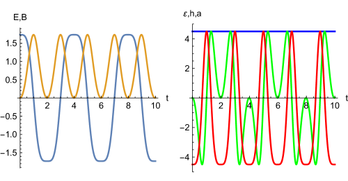
Figure 1: Yang-Mills fields in our homogeneous and isotropic test case before its coupling to an IR-CFT. Left: The electric (blue) and magnetic (orange) fields with $C=3^{1/4}$ and $t_{0}=0$ in (20). Right: The conserved energy density $\varepsilon$ (blue) and the oscillating quantities $h=-\mathcal{L}_{\rm YM}$ (red) and $a=-\mathbf{E}^{a}\cdot\mathbf{B}^{a}$ (green).

The expressions for the preserved energy and pressure read

$$\mathcal{\varepsilon}=3p=\frac{1}{2}\left(\mathbf{E}^{a2}+\mathbf{B}^{a2}\right)=\frac{3}{2}\left(f^{\prime}(t)^{2}+f(t)^{4}\right).$$ (19)

The equation of the anharmonic oscillator (18) has a closed-form solution in terms of the Jacobi elliptic function

$$f(t)=C\,\mathrm{sn}(C(t-t_{0})|-1)$$ (20)

which is a double periodic function in the complex plane. Along the real axis one has sinusoidal oscillations with the peculiarity that around a zero there is a linear term but no cubic term because the potential is flat at the origin, $\mathrm{sn}(t|-1)=t-t^{5}/10+O(t^{9})$.

In the left panel of Fig. 1 the color-electric and color-magnetic fields are shown for initial conditions corresponding to $C=3^{1/4}$ and $t_{0}=0$ in (20). ($C$ is chosen such as to match the numerical solutions of Fig. 3 in units where $Q_{s}=1$ and in the limit that the entire energy is in the Yang-Mills fields.) The right panel shows the conserved energy density $\varepsilon$ and the oscillating quantities $h=-\frac{1}{2}(\mathbf{E}^{a}\cdot\mathbf{E}^{a}-\mathbf{B}^{a}\cdot\mathbf{B}^{a})$ and $a=-\mathbf{E}^{a}\cdot\mathbf{B}^{a}$. The negative action density $h$ is seen to oscillate between $-\varepsilon$ and $+\varepsilon$ without having a mean value of zero; the topological charge density $a$ has the same extremal values with a more complicated but symmetric oscillation pattern.

When coupled to the IR-CFT, the energy-momentum tensor of the Yang-Mills theory is no longer conserved separately. In order to use the above ansatz in a semi-holographic setup in the simplest way, we want to find an appropriate exact gravity solution that allows for a time dependent boundary metric of the form (6a).

3.2 IR-CFT sector: Analytic gravity solution

The simplest IR-CFT configuration that we can couple self-consistently to the classical Yang-Mills system considered above is one that retains the same symmetries, namely homogeneity and isotropy. A remarkable simplification happens when we consider the case in which $\alpha$ and $\beta$ in (6) vanish. The only non-trivial marginal deformation of the IR-CFT in this case is via the background metric (that is identified with the boundary metric of the dual gravity solution), which takes the form:

$$g^{\rm(b)}_{\mu\nu}=\eta_{\mu\nu}+\frac{\gamma}{Q_{s}^{4}}t_{\mu\nu}=\mathrm{diag}\left(-1+\frac{3\gamma}{Q_{s}^{4}}p(t),1+\frac{\gamma}{Q_{s}^{4}}p(t),1+\frac{\gamma}{Q_{s}^{4}}p(t),1+\frac{\gamma}{Q_{s}^{4}}p(t)\right).$$ (21)

Note that in order to preserve the signature and regularity of the background metric the coupling $\gamma$ must lie in the interval:

$$-\frac{Q_{s}^{4}}{p(t)}<\gamma<\frac{Q_{s}^{4}}{3p(t)}.$$ (22)

A crucial simplification for the following calculation is that the metric (21) is conformally flat.

As mentioned above, we impose homogeneity and isotropy on the IR-CFT energy-momentum tensor $\mathcal{T}^{\mu\nu}$. When the IR-CFT is holographic, it follows that the dual geometry should also have homogeneity and isotropy, since both the data, namely the boundary metric and $\mathcal{T}^{\mu\nu}$, which determine the solution, have these properties. Furthermore, as the hard-soft couplings $\alpha$ and $\beta$ are switched off, the bulk dilaton and axion fields vanish. This allows us to apply Birkhoff’s theorem, according to which the bulk metric should be locally diffeomorphic to the standard AdS-Schwarzschild black brane solution:

$$\mathrm{d}s^{2}=-\left(r^{2}-\frac{c}{r^{2}}\right)\mathrm{d}v^{2}+\left(r^{2}-\frac{c}{r^{2}}\right)^{-1}\mathrm{d}r^{2}+r^{2}\left(\mathrm{d}x^{2}+\mathrm{d}y^{2}+\mathrm{d}z^{2}\right),$$ (23)

where $c$ is related to the mass of the black brane. In our case, $c$ will be a free parameter related to the IR-CFT initial conditions (particularly the initial energy in this sector).

The IR-CFT state dual to the AdS-Schwarzschild black brane (23) is the thermal state (with the temperature $T$ determined by the mass parameter $c$) living in flat Minkowski space, which is the boundary metric of this gravity solution. Since we are interested in a homogeneous and isotropic IR-CFT state that lives in the metric (21), we should apply a bulk diffeomorphism which is non-trivial at the boundary and is such that the boundary metric transforms from $\eta_{\mu\nu}$ to (21). At the boundary, this bulk diffeomorphism should reduce to a precise combination of a Weyl transformation and a diffeomorphism of the time coordinate, since (21) is conformally flat. Indeed, such a bulk diffeomorphism is unique (once we also choose the final gauge), and is explicitly given in Appendix B. In Appendix B we also calculate the canonical charge of the bulk space time showing that up to anomalous effects the total gravitational energy is constant and equals that of the AdS-Schwarzschild black hole with a flat boundary. Applying this bulk diffeomorphism, we obtain our desired gravity solution from which we can obtain $\hat{\mathcal{T}}^{\mu\nu}$ defined in (9) in the dual IR-CFT state, through the standard holographic dictionary that states:

$$\mathcal{T}^{\mu\nu}=\frac{2}{\sqrt{-g^{\rm{(b)}}}}\frac{\delta S_{\mathrm{EH}}^{\mathrm{on-shell}}}{\delta g^{\rm{(b)}}_{\mu\nu}},$$ (24)

where $S_{\mathrm{EH}}^{\mathrm{on-shell}}$ denotes the holographically renormalized on-shell five-dimensional Einstein-Hilbert action. Since $g^{\rm{(b)}}_{\mu\nu}$ in (21) is conformally flat, the energy-momentum tensor $\mathcal{T}^{\mu\nu}$ is not renormalization-scheme dependent.

At this stage, it is interesting to note that we can also derive the form of the required homogeneous and isotropic $\mathcal{T}^{\mu\nu}$ in the IR-CFT via a general alternative method, which works also when the IR-CFT is not holographic. We still need to assume that, except for a non-trivial background metric, all other background sources vanish, which requires us to put the couplings $\alpha$ and $\beta$ to zero. The only additional assumption that we need to put in is that the IR-CFT state is the (time-dependent) conformal (plus a coordinate) transformation of the thermal state (with an arbitrary temperature), where the transformation brings $\eta_{\mu\nu}$ to the desired background metric (21) determined by the classical Yang-Mills fields. Since we cannot take the benefit of Birkhoff’s theorem that applies on the gravity side in the large $N$ limit in holographic CFTs, we cannot say that this should be the unique homogeneous and isotropic IR-CFT living in this background metric. Nevertheless,

we can self-consistently assume that the IR-CFT state is the conformally transformed thermal state.

Under conformal transformation, $\mathcal{T}^{\mu\nu}$ transforms as a contravariant tensor of rank two and with Weyl weight two in a CFT, up to a state-independent and renormalization-scheme independent anomalous term. In a 4D CFT, this anomalous term in a conformally flat background metric is given by (see for example PhysRevD.16.1712 ; Herzog:2013ed ):

$$\mathcal{T}^{{\rm(an)}\mu\nu}=-\frac{a_{4}}{(4\pi)^{2}}\left(g^{\mu\nu}\left(\frac{R^{2}}{2}-R_{\alpha\beta}R^{\alpha\beta}\right)+2R^{\mu\lambda}R^{\nu}_{\phantom{\mu}\lambda}-\frac{4}{3}RR^{\mu\nu}\right),$$ (25)

where $a_{4}$ is the central charge associated with the Euler density. Thus, we need to add the above anomalous piece (evaluated in the metric (21) to the covariant piece obtained after conformal transformation to compute the desired IR-CFT $\mathcal{T}^{\mu\nu}$. In a holographic CFT, as expected on general grounds, we get the same result in this method as obtained via the direct application of the holographic dictionary on the dual gravity solution as mentioned before, by using

$$a_{4}=\frac{N_{c}^{2}}{4}.$$ (26)

The above is a universal result for a strongly coupled large $N$ holographic CFT.

Either by using the standard holographic dictionary (for details see Appendix B) or via the simplified procedure mentioned above, we obtain the (diagonal) components of $\hat{\mathcal{T}}^{\mu\nu}$ as follows:

$$\hat{\mathcal{E}} := \hat{\mathcal{T}}^{tt}=\frac{N_{c}^{2}}{2\pi^{2}}\left(\frac{3c}{4r_{\textrm{\tiny$\rm(0)$}}(t)^{2}v_{\textrm{\tiny$\rm(0)$}}^{\prime}(t)}+\frac{3r_{\textrm{\tiny$\rm(0)$}}^{\prime}(t)^{4}}{16r_{\textrm{\tiny$\rm(0)$}}(t)^{6}v_{\textrm{\tiny$\rm(0)$}}^{\prime}(t)^{5}}\right),$$

$$\hat{\mathcal{P}} := \hat{\mathcal{T}}^{xx}=\hat{\mathcal{T}}^{yy}=\hat{\mathcal{T}}^{zz}=$$

$$= \frac{N_{c}^{2}}{2\pi^{2}}\left\{\frac{cv_{\textrm{\tiny$\rm(0)$}}^{\prime}(t)}{4r_{\textrm{\tiny$\rm(0)$}}(t)^{2}}+\frac{r_{\textrm{\tiny$\rm(0)$}}^{\prime}(t)^{2}\left[4r_{\textrm{\tiny$\rm(0)$}}(t)r_{\textrm{\tiny$\rm(0)$}}^{\prime}(t)v_{\textrm{\tiny$\rm(0)$}}^{\prime\prime}(t)+r_{\textrm{\tiny$\rm(0)$}}(t)\left(5r_{\textrm{\tiny$\rm(0)$}}^{\prime}(t)^{2}-4r_{\textrm{\tiny$\rm(0)$}}(t)r_{\textrm{\tiny$\rm(0)$}}^{\prime\prime}(t)\right)\right]}{16r_{\textrm{\tiny$\rm(0)$}}(t)^{6}v_{\textrm{\tiny$\rm(0)$}}^{\prime}(t)^{4}}\right\},$$

with

$$r_{\textrm{\tiny$\rm(0)$}}(t)=\sqrt{1+(\gamma/Q_{s}^{4})p(t)}~{},$$

$$v_{\textrm{\tiny$\rm(0)$}}^{\prime}(t)=\sqrt{\frac{1-(\gamma/Q_{s}^{4})3p(t)}{1+(\gamma/Q_{s}^{4})p(t)}}~{}.$$ (28)

The terms proportional to $c$ are simply the result of the transformation of the energy-momentum tensor density of the AdS-Schwarzschild space-time with flat boundary conditions and thus only involve the Yang-Mills pressure $p(t)$ without derivatives. This part of the energy-momentum tensor is still traceless and (covariantly) conserved on its own with respect to the metric $g^{\rm(b)}_{\mu\nu}$. Furthermore, it is also the most relevant contribution to the energy-momentum density in a small $\gamma/Q_{s}^{4}$ expansion which reads

$$\hat{\mathcal{E}} = \frac{3cN_{c}^{2}}{8\pi^{2}}\left[1+\frac{\gamma}{Q_{s}^{4}}p(t)+3\left(\frac{\gamma}{Q_{s}^{4}}p(t)\right)^{2}\right]+\mathcal{O}\left[\left(\frac{\gamma}{Q_{s}^{4}}p(t)\right)^{3}\right]~{},$$ (29)

$$\hat{\mathcal{P}} = \frac{cN_{c}^{2}}{8\pi^{2}}\left[1-3\frac{\gamma}{Q_{s}^{4}}p(t)+3\left(\frac{\gamma}{Q_{s}^{4}}p(t)\right)^{2}\right]+\mathcal{O}\left[\left(\frac{\gamma}{Q_{s}^{4}}p(t)\right)^{3}\right].$$ (30)

As we shall see below, only the combination $(\gamma/Q_{s}^{4})(\hat{\mathcal{E}}+\hat{\mathcal{P}})$ contributes in the equations of motion of the semi-holographic model. Therefore the leading-order effect of the back-reaction on the Yang-Mills fields, mediated by the deformation of the IR-CFT due to the Yang-Mills fields which determine $p(t)$, is of order $(\gamma/Q_{s}^{4})^{3}$. To leading order $\gamma/Q_{s}^{4}$, the IR-CFT acts on the Yang-Mills fields through the soft thermal bath that one starts with by choosing $c\neq 0$.

The terms independent of $c$ in Eq. (3.2) are due to the nonvanishing Ricci tensor of $g^{\textrm{\tiny$\rm(b)$}}_{\mu\nu}$ and their trace gives the conformal anomaly, which in our case is determined solely by the Euler-density associated with $g^{\textrm{\tiny$\rm(b)$}}_{\mu\nu}$. These only contribute at non-stationary points of the Yang-Mills pressure, i.e., for $p^{\prime}(t)\neq 0$, and are of order $(\gamma/Q_{s}^{4})^{3}$.

3.3 Coupling the UV with the IR sector

We now have all the ingredients at hand to test our modified semi-holography proposal. The equations of motion (10) for the coupled system with a homogeneous and isotropic ansatz for the UV-Yang-Mills gauge fields (17) coupled to a homogeneous and isotropic IR energy-momentum tensor become

$$f^{\prime\prime}(t)+2\frac{1-\frac{1}{2}\frac{\gamma}{Q_{s}^{4}}(\hat{\mathcal{E}}+\hat{\mathcal{P}})}{1+\frac{1}{2}\frac{\gamma}{Q_{s}^{4}}(\hat{\mathcal{E}}+\hat{\mathcal{P}})}f(t)^{3}+\frac{1}{2}\frac{\gamma}{Q_{s}^{4}}\frac{(\hat{\mathcal{E}}+\hat{\mathcal{P}})^{\prime}}{1+\frac{1}{2}\frac{\gamma}{Q_{s}^{4}}(\hat{\mathcal{E}}+\hat{\mathcal{P}})}f^{\prime}(t)=0,$$ (31)

where $\hat{\mathcal{E}}$ and $\hat{\mathcal{P}}$ are given by (3.2). It is remarkable that only the combination $\hat{\mathcal{E}}+\hat{\mathcal{P}}$ is needed, which is given in closed form by

$$\hat{\mathcal{E}}+\hat{\mathcal{P}} = \frac{N_{c}^{2}}{2\pi^{2}}\frac{c}{\sqrt{1-3\bar{\gamma}p(t)}[1+\bar{\gamma}p(t)]^{3/2}}$$ (32)

$$+\frac{N_{c}^{2}}{2\pi^{2}}\frac{\bar{\gamma}^{3}p^{\prime}(t)^{2}\left(2[1+\bar{\gamma}p(t)][3\bar{\gamma}p(t)-1]p^{\prime\prime}(t)-\bar{\gamma}[1+6\bar{\gamma}p(t)]p^{\prime}(t)^{2}\right)}{64[1-3\bar{\gamma}p(t)]^{5/2}[1+\bar{\gamma}p(t)]^{7/2}}\;,$$

where we introduced the abbreviation $\bar{\gamma}=\gamma/Q_{s}^{4}$.

The full energy density for our test case is obtained by taking the zeroth component of the energy-momentum tensor (12), which can be expressed in the following convenient form:

$$E=\varepsilon+\hat{\mathcal{E}}\left(1-\frac{\gamma}{Q_{s}^{4}}\varepsilon\right)+\frac{3}{2}\frac{\gamma}{Q_{s}^{4}}\left(\hat{\mathcal{E}}+\hat{\mathcal{P}}\right)f^{\prime}(t)^{2}.$$ (33)

In order to solve (31), which is an ordinary fourth-order differential equation when $p(t)$ in $\hat{\mathcal{E}}+\hat{\mathcal{P}}$ is expressed in terms of $f(t)$ through (19), we will use the iterative algorithm proposed in Iancu:2014ava and test its usability. By interpreting $\hat{\mathcal{E}}+\hat{\mathcal{P}}$ as a fixed external source, which is updated after each iteration, this reduces to a second-order differential equation for $f(t)$. While in principle this method should not be necessary for our test case, in practice we have not been able to find regular solutions of the above highly nonlinear fourth-order equation other than by following the iterative procedure. Moreover, one has to keep in mind that for more complicated dynamics, e.g., for an anisotropic situation or for $\alpha,\beta\neq 0$, the expression of $\hat{\mathcal{T}}^{\mu\nu}$ in terms of the Yang-Mills fields (here $f(t)$) will not be explicitly known.

Eq. (31) is reminiscent of an equation of motion for an anharmonic oscillator where the coefficient of the $f(t)^{3}$ term determines the frequency of the oscillations, whereas the last term acts as (anti-)damping term. In order to obtain regular oscillating solutions the frequencies are constrained to take real values.

Before discussing the full numerical result, we describe the first two steps of the algorithm, allowing us to extract analytic behavior which approximates the full solution very well for sufficiently small values of $N_{c}^{2}\gamma c/(2\pi^{2}Q_{s}^{4})$. In the first step we set $\hat{\mathcal{E}}+\hat{\mathcal{P}}=0$ which amounts to the solution for $f(t)$ we have already discussed in section 3.1 and for which $p(t)=p_{\textrm{\tiny$\rm 0$}}:=p(0)$. Inserting the latter into (32), the updated source now reads

$$\hat{\mathcal{E}}_{\textrm{\tiny$\rm 0$}}+\hat{\mathcal{P}}_{\textrm{\tiny$\rm 0$}}=\frac{N_{c}^{2}}{2\pi^{2}}\frac{c}{\sqrt{1-3\frac{\gamma}{Q_{s}^{4}}p_{\textrm{\tiny$\rm 0$}}}[1+\frac{\gamma}{Q_{s}^{4}}p_{\textrm{\tiny$\rm 0$}}]^{3/2}},$$ (34)

which is larger than $N_{c}^{2}/(2\pi^{2})c$ irrespective of the sign of $\gamma$.

For a special choice of initial conditions, either $f^{\prime}(0)=\pm\sqrt{2p_{\textrm{\tiny$\rm 0$}}}$, $f(0)=0$ or $f^{\prime}(0)=0$, $f(0)=\pm(2p_{\textrm{\tiny$\rm 0$}})^{1/4}$, it follows automatically that $\hat{\mathcal{E}}+\hat{\mathcal{P}}$ at the initial time $t=0$ always takes the value given in (34).

In the second step of the iterative process the derivative of $\hat{\mathcal{E}}+\hat{\mathcal{P}}$ still vanishes and we only have to solve the second order differential equation

$$f^{\prime\prime}(t)+2\frac{1-\frac{1}{2}\frac{\gamma}{Q_{s}^{4}}(\hat{\mathcal{E}}_{\textrm{\tiny$\rm 0$}}+\hat{\mathcal{P}}_{\textrm{\tiny$\rm 0$}})}{1+\frac{1}{2}\frac{\gamma}{Q_{s}^{4}}(\hat{\mathcal{E}}_{\textrm{\tiny$\rm 0$}}+\hat{\mathcal{P}}_{\textrm{\tiny$\rm 0$}})}f(t)^{3}=0\;.$$ (35)

Choosing the initial conditions $f(0)=(2p_{\textrm{\tiny$\rm 0$}})^{(1/4)}$ and $f^{\prime}(0)=0$, again an analytic solution in terms of Jacobi elliptic functions can be found,

$$f(t) = (2p_{\textrm{\tiny$\rm 0$}})^{\frac{1}{4}}\mathrm{cd}(\omega t|-1)\;,$$

$$\omega := 4K(-1)\nu=(2p_{\textrm{\tiny$\rm 0$}})^{\frac{1}{4}}\left(\frac{1-\frac{1}{2}\frac{\gamma}{Q_{s}^{4}}(\hat{\mathcal{E}}_{\textrm{\tiny$\rm 0$}}+\hat{\mathcal{P}}_{\textrm{\tiny$\rm 0$}})}{1+\frac{1}{2}\frac{\gamma}{Q_{s}^{4}}(\hat{\mathcal{E}}_{\textrm{\tiny$\rm 0$}}+\hat{\mathcal{P}}_{\textrm{\tiny$\rm 0$}})}\right)^{\frac{1}{2}}\;,$$ (36)

where $K(-1)\approx 1.31$ denotes the complete elliptic integral of the first kind, which is the quarter period of the Jacobi elliptic function, e.g. $\mathrm{sn}(x|-1)=\mathrm{sn}\left(x+4K(-1)|-1\right)$. Accordingly we may call $\nu$ the frequency of the anharmonic oscillations. As already mentioned, demanding a regular solution imposes a reality condition on $\nu$, which in turn puts bounds to the value of $N_{c}^{2}\gamma c/(2\pi^{2}Q_{s}^{4})$ in addition to those put on $\gamma/Q_{s}^{4}p_{\textrm{\tiny$\rm 0$}}$ guaranteeing regularity of $g^{\textrm{\tiny$\rm(b)$}}_{\mu\nu}$. The allowed parameter space is illustrated in Fig. 2. The total initial energy of the full semi-holographic system for this choice of initial conditions is given by

$$E = \varepsilon(0)+\hat{\mathcal{E}}(0)\left(1-\frac{\gamma}{Q_{s}^{4}}\varepsilon(0)\right)=3p_{\textrm{\tiny$\rm 0$}}+\frac{3N_{c}^{2}c}{8\pi^{2}}\sqrt{\frac{1-3\frac{\gamma}{Q_{s}^{4}}p_{\textrm{\tiny$\rm 0$}}}{1+\frac{\gamma}{Q_{s}^{4}}p_{\textrm{\tiny$\rm 0$}}}},$$ (37)

which remains true to all orders of the iterative algorithm.

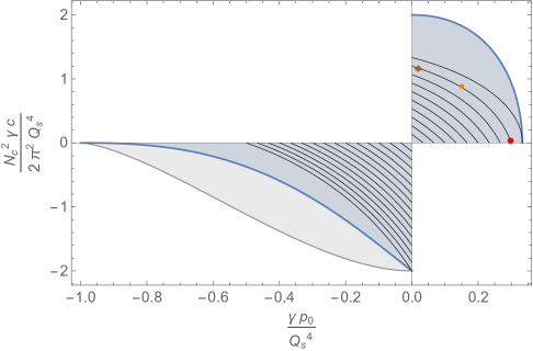
Figure 2: The allowed regions (shaded) for the values of $\frac{N_{c}^{2}\gamma c}{2\pi^{2}Q_{s}^{4}}$ and $\frac{\gamma p_{\textrm{\tiny$\rm 0$}}}{Q_{s}^{4}}$. In the lower left quadrant the lower boundary curve (grey) is obtained from the reality condition for $\omega$ in (36), i.e. after the first iteration. The more restrictive boundary curve (blue) above is obtained from demanding the regularity of the metric after the second iteration step. The thin lines correspond to constant values of the total energy $\frac{\gamma E}{Q_{s}^{4}}=i/10$, with $i=1,\dots 10$ in the first quadrant and $i=-1,\dots-15$ in the third quadrant. The point, the square and the diamond correspond to the values used for the numerical evaluations.

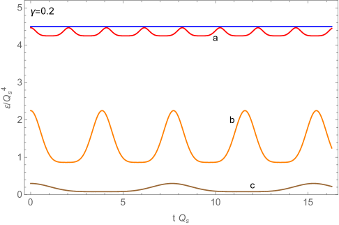
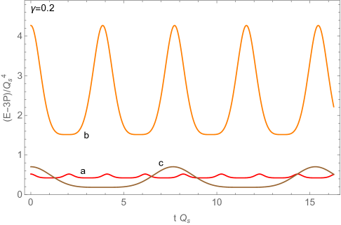
Figure 3: The numerical solution of (31) in terms of the Yang-Mills energy density $\varepsilon$ (upper panel) and the negative trace of the full energy-momentum tensor, $-T^{\mu\nu}\eta_{\mu\nu}=E-3P$, (lower panel) for $p^{\textrm{\tiny$\rm(a)$}}_{\textrm{\tiny$\rm 0$}}/Q_{s}^{4}=1.49$, $p^{\textrm{\tiny$\rm(b)$}}_{\textrm{\tiny$\rm 0$}}/Q_{s}^{4}=0.75$, $p^{\textrm{\tiny$\rm(c)$}}_{\textrm{\tiny$\rm 0$}}/Q_{s}^{4}=0.1$ with $\gamma=0.2$ and total (conserved) energy density $E/Q_{s}^{4}=4.5$, marked by the blue line in the upper panel. The three solutions (a), (b), (c) involve increasing values of $c$, and $\varepsilon$ constitutes a correspondingly smaller fraction of the total energy density $E$ (upper panel). The trace term $E-3P$ in the lower panel can be thought of as an “interaction measure” of the UV and IR sector which in our test case vanishes exactly in the two extreme cases $\varepsilon=E$ and $\varepsilon=0$.

Starting with the third step of the iterative algorithm requires to solve the second order equation for $f(t)$ numerically. Note that for positive $\gamma$ we find $p(t)\leqslant p_{\textrm{\tiny$\rm 0$}}$, while for negative $\gamma$ we find $p(t)\geqslant p_{\textrm{\tiny$\rm 0$}}$, meaning that for negative $\gamma$ the allowed region for the values of $N_{c}^{2}\gamma c/(2\pi^{2}Q_{s}^{4})$ is further restricted in order to ensure regularity of the metric as shown by the blue line in Fig. 2. There we also show lines of constant values of $\gamma E/Q_{s}^{4}$ that completely fit within the restricted regions. For positive $\gamma$ we find $\gamma E/Q_{s}^{4}\leqslant 1$ and for negative $\gamma$ this condition amounts to $\gamma E/Q_{s}^{4}\geqslant-1.5$.

In Fig. 3 we present the numerical solution for three different choices of $p_{\textrm{\tiny$\rm 0$}}/Q_{s}^{4}$ with $\gamma=0.2$ and constant energy $E/Q_{s}^{4}=4.5$: $p^{\textrm{\tiny$\rm(a)$}}_{\textrm{\tiny$\rm 0$}}/Q_{s}^{4}=1.49$, $p^{\textrm{\tiny$\rm(b)$}}_{\textrm{\tiny$\rm 0$}}/Q_{s}^{4}=0.75$, $p^{\textrm{\tiny$\rm(c)$}}_{\textrm{\tiny$\rm 0$}}/Q_{s}^{4}=0.1$. These choices are depicted by the colored markers in Fig. 2.

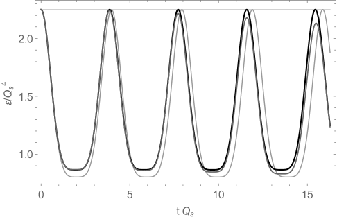
Figure 4: Convergence of the iterative solution to case (b) of Fig. 3, with increasing darkness of the grey lines for increasing order of the iteration. From the fourth iteration onwards the changes are too small to be visible in this plot.

In the upper panel of Fig. 3, the blue horizontal line marks the total energy density, and the three oscillating lines give the Yang-Mills part of it for the three choices of $p_{\textrm{\tiny$\rm 0$}}$. The difference to the total energy density is the oppositely oscillating component contained in the soft modes together with their interaction energy with the hard modes.

Fixing the energy density in (37) and varying $p_{\textrm{\tiny$\rm 0$}}/Q_{s}^{4}$ for the three solutions means that we have to adjust the parameter $c$, which is related to the black holes mass, accordingly. Going from higher to lower values in $p_{\textrm{\tiny$\rm 0$}}$ with fixed $E$ means that $c$ is increased and the black hole made larger. (The case $c=0$ corresponds to the trivial solution where one has exactly $p_{\textrm{\tiny$\rm 0$}}=E/3$.) In a more realistic setup where the gravity solution is dynamical and not just a gauge transformation of the AdS-Schwarzschild black hole, we expect that due to the interaction between the hard and soft sector the growing black hole draws energy from the hard modes as the system thermalizes. The UV energy density thus may shrink and get deposited in the IR-sector. This is mimicked here by choosing different initial conditions. Interestingly, with the choice of positive $\gamma$ in the example shown in Fig. 3, the wavelength of the oscillation increases as the Yang-Mills energy density decreases, which is not the case for negative $\gamma$. Furthermore, for positive $\gamma$ the trace term $E-3P$ depicted in the lower panel of Fig. 3 is always positive, consistent with lattice results of QCD thermodynamics Boyd:1996bx ; Borsanyi:2010cj , where $E-3P$ is often called the “interaction measure”.

We applied two criteria in order to decide whether the algorithm converges. The first is of course to check whether equation (31) evaluated at the solution for $f(t)$ is satisfied sufficiently, which is nontrivial, since the solution for $f(t)$ was obtained for source terms evaluated with the solution of the previous iteration step. The second criterion is that the total energy evaluated at the solution for $f(t)$ is sufficiently close to the value prescribed in Eq. (37) respectively. In the solution presented in Fig. 3 both criteria were satisfied up to order $10^{-7}$ which is smaller than any term appearing in (31) in particular the one involving the fourth order derivative of $f(t)$.

Figure 4 shows the convergence of the iterative solution for the case (b). From the fourth iteration onwards, there is no visible change of the numerical result.

4 Conclusions

In this paper we presented an improved and extended version of the semi-holographic model proposed in Iancu:2014ava . The idea behind semi-holography is to construct a phenomenological model for heavy-ion collisions that is able to incorporate the interaction between the weakly coupled UV and the strongly coupled IR-sector. This is done by assuming that the UV sector is given by over-occupied gluon modes admitting a description in terms of classical Yang-Mills fields, while the strongly coupled IR-sector is described by a conformal field theory with a holographic dual.

We presented a new action where such a mechanism can be implemented, and we constructed the full energy-momentum tensor of the coupled theory which is locally conserved and thus can track the energy transfer between the two sectors. The full energy-momentum tensor consists of the standard Yang-Mills theory expression plus contributions derived from the effective action of the conformal field theory which is deformed by the marginal operators of the Yang-Mills theory. The latter contributions thus comprise both purely soft and soft-hard ones, which however cannot be disentangled unambiguously; only the thermal part of the soft sector has a well-defined meaning in terms of the black hole horizon of the holographic gravity dual.

Moreover, we have presented first numerical tests of the iterative procedure proposed for solving the evolution of the semi-holographic model. By assuming homogeneity and isotropy we were able to construct a simple test case with closed analytic solutions for the two decoupled sectors. Coupling them together via the tensorial coupling only, we numerically solved for the evolution of the fields and observed quick convergence of the algorithm and observed energy exchange between the Yang-Mills part and the conformal field theory with constant total energy. This is already a nontrivial result and is a proof of principle of this semi-holography proposal.

Of course, due to the simplicity and high symmetry of this test case we could not observe thermalization. This was expected because without any propagating degrees of freedom our gravity solution does not incorporate dynamical black hole formation, only time-dependent diffeomorphisms of a pre-existing black hole, i.e., the black hole temperature and the entropy measured by the surface gravity and the horizon area respectively are not altered. In order for the system to relax, more degrees of freedom must be included. This can be done by introducing anisotropy in the space-time along the lines of Chesler:2008hg and also making the Yang-Mills fields anisotropic. It is then expected that the black hole is able to draw energy from the hard modes and that isotropization occurs. Another possibility is to stay isotropic and to turn on one or both of the scalar fields on the gravity side coupled to the Lagrange density and the Pontryagin density on the field theory side, respectively. The latter would be particularly interesting in view of anomalous transport phenomena such as the chiral magnetic effect Kharzeev:2015znc and also with regard to the results of Ref. Rebhan:2011vd on the shear viscosity in strongly coupled anisotropic systems. We plan to tackle these more complicated scenarios in future work.

Depending on the initial conditions and/or the values of $\alpha$, $\beta$ and $\gamma$, various different scenarios of thermalization may appear, e.g., the hard modes may eventually drain their energy almost completely to the black hole, or the hard modes might retain a significant fraction of their energy even at late time, while the full energy-momentum tensor (12) approaches a diagonal form. In the latter case, we would expect that the effective hydrodynamic description which results from the fluid/gravity correspondence Rangamani:2009xk will not suffice to describe the late stage of the evolution prior to hadronization. Since at late times, where the relatively hard gluons are less densely populated, a kinetic theory approach may be more suitable than the classical field theory (glasma) description, it would also be interesting to understand  how to couple kinetic theory to a holographic CFT in our semi-holographic framework. In this context, it may be useful to follow Muller:2015maa ; Yang:2015bva , where a similar attempt has been made in context of constructing a kinetic theory of leptons and photons when the latter are interacting with strongly coupled QCD matter. This could e.g. have an important bearing on the $v_{2}$ photon puzzle Adare:2011zr ; Lohner:2012ct that pertains to the late stage of the evolution.

In the future, we may also hope to determine the (so far free) hard-soft coupling constants $\alpha$, $\beta$, and $\gamma$ in terms of $\alpha_{s}(Q_{s})$ to a certain degree of approximation, by using renormalisation group techniques as discussed in Behr:2015yna ; Behr:2015aat . In this case, the semi-holographic model could eventually lead to sharp predictions.

Appendix A Conservation of the full energy-momentum tensor

In this Appendix we show that the full energy-momentum tensor

$$T^{\mu\nu} = t^{\mu\nu}$$ (38)

$$+\hat{\mathcal{T}}^{\alpha\beta}\left\{\delta_{(\alpha}^{\mu}\delta_{\beta)}^{\nu}-\frac{\gamma}{Q_{s}^{4}N_{c}}\left[\mathrm{Tr}(F_{\alpha}^{\ \mu}F_{\beta}^{\ \nu})-\frac{1}{2}\eta_{\alpha\beta}\mathrm{Tr}(F^{\mu\rho}F^{\nu}_{\ \rho})+\frac{1}{4}\delta_{(\alpha}^{\mu}\delta_{\beta)}^{\nu}\mathrm{Tr}(F^{2})\right]\right\}$$

$$-\frac{\beta}{Q_{s}^{4}N_{c}}\hat{\mathcal{H}}\,\mathrm{Tr}(F^{\mu\alpha}F^{\nu}_{\ \alpha})-\frac{\alpha}{Q_{s}^{4}}\eta^{\mu\nu}\hat{\mathcal{A}}\,a$$

is conserved to all orders in the coupling constants. Let us first revisit the divergence of $t^{\mu\nu}$ for completeness:

$$\partial_{\mu}t^{\mu\nu}=\frac{1}{N_{c}}\mathrm{Tr}[(D_{\mu}F^{\mu\rho})F^{\nu}_{\ \rho}]$$ (39)

where we used

$$\frac{1}{N_{c}}\mathrm{Tr}(F^{\mu\rho}D_{\mu}F^{\nu}_{\ \rho}-\frac{1}{2}F^{\rho\mu}D^{\nu}F_{\rho\mu})=-\frac{1}{2N_{c}}\mathrm{Tr}[F^{\rho\mu}\eta^{\nu\tau}(D_{\tau}F_{\rho\mu}+D_{\rho}F_{\mu\tau}+D_{\mu}F_{\tau\rho})]=0,\qquad$$ (40)

due to the Bianchi identity. In order to show conservation of the full energy-momentum tensor we need to rewrite the individual interaction terms. The first term can be brought in the following form

$$-\frac{\gamma}{Q_{s}^{4}N_{c}}\partial_{\mu}[\hat{\mathcal{T}}^{\alpha\beta}\mathrm{Tr}(F_{\alpha}^{\ \mu}F_{\beta}^{\ \nu})]$$

$$=-\frac{\gamma}{Q_{s}^{4}N_{c}}\mathrm{Tr}[D_{\mu}(F_{\ \alpha}^{\mu}\hat{\mathcal{T}}^{\alpha\beta})F^{\nu}_{\ \beta}]-\frac{\gamma}{Q_{s}^{4}N_{c}}\mathrm{Tr}(\hat{\mathcal{T}}^{\alpha\beta}F_{\alpha}^{\ \mu}D_{\mu}F_{\beta}^{\ \nu}),$$ (41)

where the first term on the right-hand side appears in the equations of motion (10). By using the same trick as for the YM energy-momentum tensor the second term becomes

$$\frac{\gamma}{2Q_{s}^{4}N_{c}}\partial_{\mu}[\hat{\mathcal{T}}^{\alpha\beta}\eta_{\alpha\beta}\mathrm{Tr}(F^{\mu\rho}F^{\nu}_{\ \rho})]$$

$$=\frac{\gamma}{2Q_{s}^{4}N_{c}}\mathrm{Tr}[D_{\mu}(\hat{\mathcal{T}}F^{\mu\beta})F^{\nu}_{\ \beta}]+\frac{\gamma}{8Q_{s}^{4}N_{c}}\hat{\mathcal{T}}\partial^{\nu}\mathrm{Tr}(F^{2}),$$ (42)

where also the first term appears in the equations of motion. The third term is

$$-\frac{\gamma}{4Q_{s}^{4}N_{c}}\partial_{\mu}[\hat{\mathcal{T}}^{\mu\nu}\mathrm{Tr}(F^{2})]=\frac{\gamma}{Q_{s}^{4}}\partial_{\mu}\{\hat{\mathcal{T}}^{\mu\alpha}[t_{\alpha}^{\ \nu}-\frac{1}{N_{c}}\mathrm{Tr}(F_{\alpha}^{\ \beta}F^{\nu}_{\ \beta})]\}\qquad$$

$$=-\frac{\gamma}{Q_{s}^{4}N_{c}}\mathrm{Tr}[D_{\mu}(\hat{\mathcal{T}}^{\mu\alpha}F_{\alpha}^{\ \beta})F^{\nu}_{\ \beta}]+\frac{\gamma}{Q_{s}^{4}}\partial_{\mu}(\hat{\mathcal{T}}^{\mu\alpha}t_{\alpha}^{\ \nu})-\frac{\gamma}{2Q_{s}^{4}}\hat{\mathcal{T}}^{\alpha\beta}\partial^{\nu}t_{\alpha\beta}$$

$$-\frac{\gamma}{8Q_{s}^{4}N_{c}}\hat{\mathcal{T}}\partial^{\nu}\mathrm{Tr}(F^{2})+\frac{\gamma}{Q_{s}^{4}N_{c}}\mathrm{Tr}(\hat{\mathcal{T}}^{\alpha\beta}F_{\alpha}^{\ \mu}D_{\mu}F_{\beta}^{\ \nu}),$$ (43)

where the Bianchi identity was used to obtain the last two terms, which cancel the unwanted terms from (A) and (A). Again, the first term on the right hand side appears in the equations of motion.

The fourth term involves the dilaton field and is

$$-\frac{\beta}{Q_{s}^{4}N_{c}}\mathrm{Tr}[D_{\mu}(F^{\mu\beta}\hat{\mathcal{H}}F^{\nu}_{\ \beta})]=-\frac{\beta}{Q_{s}^{4}N_{c}}\mathrm{Tr}[D_{\mu}(F^{\mu\beta}\hat{\mathcal{H}})F^{\nu}_{\ \beta}]-\frac{\beta}{Q_{s}^{4}}\partial^{\nu}h\hat{\mathcal{H}},$$ (44)

where again the first term appears in the equations of motion. Similarly, the last term reads

$$-\frac{\alpha}{Q_{s}^{4}}\partial^{\nu}\left(a\hat{\mathcal{A}}\right)=-\frac{\alpha}{N_{c}Q_{s}^{4}}\partial_{\mu}\hat{\mathcal{A}}\mathrm{tr}(\tilde{F}^{\mu\beta}F^{\nu}_{\ \beta})-\frac{\alpha}{Q_{s}^{4}}\partial^{\nu}a\hat{\mathcal{A}},$$ (45)

where we used the identity

$$\frac{1}{N_{c}}\mathrm{tr}(\tilde{F}^{\mu\beta}F^{\nu}_{\ \beta})=\frac{1}{4N_{c}}\eta^{\mu\nu}\mathrm{tr}(\tilde{F}^{\alpha\beta}F_{\alpha\beta})=\eta^{\mu\nu}a.$$ (46)

To finally show the conservation of $T^{\mu\nu}$ in flat Minkowski space, we also need the Ward identity

$$\nabla^{(b)}_{\mu}\mathcal{T}^{\mu\nu}=\frac{\beta}{Q_{s}^{4}}\mathcal{H}\nabla^{(b)\nu}h+\frac{\alpha}{Q_{s}^{4}}\mathcal{A}\nabla^{(b)\nu}a$$ (47)

in the following form

$$\partial_{\mu}\hat{\mathcal{T}}^{\mu\nu}=\frac{\beta}{Q_{s}^{4}}\hat{\mathcal{H}}g^{(b)\mu\nu}\partial_{\mu}h+\frac{\alpha}{Q_{s}^{4}}\hat{\mathcal{A}}g^{(b)\mu\nu}\partial_{\mu}a-\Gamma^{\nu}_{\mu\sigma}\hat{\mathcal{T}}^{\mu\sigma},$$ (48)

where the Christoffel symbol is

$$\Gamma^{\nu}_{\mu\sigma}=\frac{\gamma}{Q_{s}^{4}}g^{(b)\nu\tau}\left(\partial_{(\mu}t_{\sigma)\tau}-\frac{1}{2}\partial_{\tau}t_{\mu\sigma}\right).$$ (49)

Putting everything together we finally arrive at

$$\partial_{\mu}T^{\mu\nu} = \frac{1}{N_{c}}\mathrm{Tr}[({EOMs})^{\beta}F^{\nu}_{\ \beta}]-\frac{\beta}{Q_{s}^{4}}\partial^{\nu}h\hat{\mathcal{H}}-\frac{\alpha}{Q_{s}^{4}}\partial^{\nu}a\hat{\mathcal{A}}$$ (50)

$$+\partial_{\mu}\hat{\mathcal{T}}^{\mu\nu}-\frac{\gamma}{2Q_{s}^{4}}\hat{\mathcal{T}}^{\alpha\beta}\partial^{\nu}t_{\alpha\beta}+\frac{\gamma}{Q_{s}^{4}}\partial_{\mu}(\hat{\mathcal{T}}^{\mu\sigma}t_{\sigma}^{\ \nu})$$

$$= \frac{1}{N_{c}}\mathrm{Tr}[({EOMs})^{\beta}F^{\nu}_{\ \beta}]+\left(g^{(b)\mu\nu}-\eta^{\mu\nu}+t^{\nu}_{\alpha}g^{(b)\alpha\mu}\right)\left(\frac{\beta}{Q_{s}^{4}}\partial_{\mu}h\hat{\mathcal{H}}+\frac{\alpha}{Q_{s}^{4}}\partial_{\mu}a\hat{\mathcal{A}}\right)$$

$$-\left[\Gamma^{\nu}_{\mu\sigma}+\frac{\gamma}{Q_{s}^{4}}t^{\nu}_{\alpha}\Gamma^{\alpha}_{\mu\sigma}-\frac{\gamma}{Q_{s}^{4}}\eta^{\nu\tau}\left(\partial_{(\mu}t_{\sigma)\tau}-\frac{1}{2}\partial_{\tau}t_{\mu\sigma}\right)\right]\hat{\mathcal{T}}^{\mu\sigma},$$

where we used the Ward identity in the second equality and where $(\text{\it EOMs})^{\beta}=0$ represents the equations of motion (10). Using matrix notation the inverse metric can be written as ($\eta^{(-1)}=\eta$)

$$g_{(b)}^{(-1)}=\left[\eta(\mathds{1}+\frac{\gamma}{Q_{s}^{4}}t)\right]^{(-1)}=\left[(\mathds{1}+\frac{\gamma}{Q_{s}^{4}}t)\right]^{(-1)}\eta,$$ (51)

and therefore

$$\eta^{\nu\tau}=g^{(b)\nu\tau}+\frac{\gamma}{Q_{s}^{4}}t^{\nu}_{\alpha}g^{(b)\alpha\tau}.$$ (52)

Inserting Eq. (52) in (50) we obtain that on-shell

$$\partial_{\mu}T^{\mu\nu}=0.$$ (53)

Appendix B Computation of the IR-CFT energy-momentum tensor

In this appendix we give some details of the computation of the result (3.2) for the IR-CFT energy-momentum tensor $\hat{\mathcal{T}}^{\mu\nu}$. We will follow the standard procedure to obtain it from the asymptotic expansion in the holographic (radial) coordinate of the metric in Fefferman-Graham gauge deHaro:2000xn . The transformation to the Fefferman-Graham gauge will affect the coordinates $r$ and $v$, $r\rightarrow r(\rho,t)$ and $v\rightarrow v(\rho,t)$, where $\rho$ denotes the holographic radial coordinate with the boundary located at $\rho=0$ and $t$ being the time coordinate of the boundary theory. The asymptotic expansion of the transformation reads

$$r(\rho,t) = \sum_{i=0}r_{\textrm{\tiny$\rm(i)$}}(t)\rho^{i-1},$$

$$v(\rho,t) = \sum_{i=0}v_{\textrm{\tiny$\rm(i)$}}(t)\rho^{i},$$ (54)

which we plug into (23) and solve for the coefficients by demanding that $g_{\rho\rho}=1/\rho^{2}$ and $g_{\rho t}=0$ to all orders in $\rho$. In addition we have to impose the condition that the induced metric on a constant-$\rho$ slice is regular at leading order. At leading order these conditions lead to $v_{\textrm{\tiny$\rm(1)$}}=0$ and to the metric

$$\mathrm{d}s^{2}=\frac{1}{\rho^{2}}\left[\mathrm{d}\rho^{2}+r_{\textrm{\tiny$\rm(0)$}}(t)^{2}\left(-v_{\textrm{\tiny$\rm(0)$}}^{\prime}(t)^{2}\mathrm{d}t^{2}+\mathrm{d}x^{2}+\mathrm{d}y^{2}+\mathrm{d}z^{2}\right)\right]+\mathcal{O}(\rho^{0}).$$ (55)

To obtain this metric we have only employed a coordinate transformation and therefore it also solves Einsteins equation with negative cosmological constant. Put differently, the transformation simply changes the rods and clocks of an asymptotic observer in a time dependent way. Matching this form of the metric to the boundary condition (21) gives

$$r_{\textrm{\tiny$\rm(0)$}}(t)=\sqrt{1+(\gamma/Q_{s}^{4})p(t)}$$

$$v_{\textrm{\tiny$\rm(0)$}}^{\prime}(t)=\sqrt{\frac{1-(\gamma/Q_{s}^{4})3p(t)}{1+(\gamma/Q_{s}^{4})p(t)}}~{}.$$ (56)

This is exactly what we wanted, because now we have a bulk geometry that is solely determined by the pressure of the Yang-Mills theory. To construct the full holographic energy-momentum tensor one also has to solve for the higher-order coefficients in the expansion (B), which can be expressed in terms of $r_{(0)},~{}v_{(0)}$ and derivatives thereof.

The energy-momentum tensor density is obtained from the well known formula deHaro:2000xn

$$\mathcal{T}^{\mu\nu}=\frac{N_{c}^{2}}{2\pi^{2}}\left\{g^{\textrm{\tiny$\rm(4)$}\mu\nu}-\frac{1}{2}g^{\textrm{\tiny$\rm(2)$}\mu\sigma}g^{\textrm{\tiny$\rm(2)$}\nu}_{\ \sigma}+\frac{1}{4}g^{\textrm{\tiny$\rm(2)$}\mu\nu}\mathrm{tr}g^{\textrm{\tiny$\rm(2)$}}-\frac{1}{8}g^{\textrm{\tiny$\rm(b)$}\mu\nu}\left[\left(\mathrm{tr}g^{\textrm{\tiny$\rm(2)$}}\right)^{2}-g^{\textrm{\tiny$\rm(2)$}\sigma\tau}g^{\textrm{\tiny$\rm(2)$}}_{\sigma\tau}\right]\right\},$$ (57)

where $g^{(2)}$ is the $\mathcal{O}(\rho^{0})$-term and $g^{(4)}$ the $\mathcal{O}(\rho^{2})$-term in the Fefferman-Graham expansion (2) of the bulk metric.

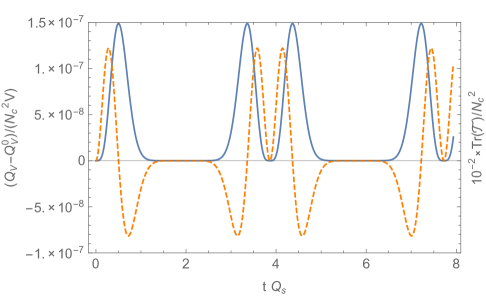
Figure 5: The solid (blue) line shows the time dependent (anomalous) contributions in (59) ($Q_{V}^{0}$ denoting the charge of the AdS-Schwarzschild black hole with flat boundary) for the case (b) of Fig. 3. The dashed (orange) line shows the evolution of $\mathrm{Tr}\,\mathcal{T}$.

From the purely gravitational perspective it is interesting to calculate the canonical charges associated with the boundary condition preserving transformations Henneaux:1985tv ; Castellani:1981us . Since the boundary metric is conformally flat, the asymptotic symmetries are still given by the conformal group $SO(2,4)$. If the boundary were flat, the vector field generating infinitesimal time translations would be $\xi_{\textrm{\tiny$\rm(t)$}}^{\mu}=(1,0,0,0)^{T}$. This in turn can be associated with a canonical charge that is interpreted as the total gravitational energy contained in the bulk of the space-time. In general, given a generator of a boundary condition preserving transformation $\xi_{\textrm{\tiny$\rm(i)$}}^{\mu}\ \in\ SO(2,4)$ the associated canonical charge reads

$$Q_{V}[\xi_{\textrm{\tiny$\rm(i)$}}]=\int_{V}\mathrm{d}^{3}x\overline{\mathcal{T}}^{t}_{\mu}\xi_{\textrm{\tiny$\rm(i)$}}^{\mu},$$ (58)

and is preserved in time up to effects due to the conformal anomaly. In (58) we introduced a regulating spatial coordinate volume $V=\Delta x\Delta y\Delta z$, since the spatial hypersurfaces in the boundary space-time are non-compact. In the case at hand the generator of time translations is promoted to a conformal Killing vector field of the transformed metric $\xi_{\textrm{\tiny$\rm(t)$}}^{\mu}=(1/v_{\textrm{\tiny$\rm(0)$}}^{\prime}(t),0,0,0)^{T}$. The charge associated with this becomes

$$Q_{V}[\xi_{\textrm{\tiny$\rm t$}}]=V\frac{3N_{c}^{2}}{16\pi^{2}}\left(4c+\frac{r_{\textrm{\tiny$\rm(0)$}}^{\prime}(t)^{4}}{r_{\textrm{\tiny$\rm(0)$}}(t)^{4}v_{\textrm{\tiny$\rm(0)$}}^{\prime}(t)^{4}}\right),$$ (59)

where the first contribution is identical to the canonical charge with flat boundary conditions. The second contribution is always positive and vanishes for $p^{\prime}(t)=0$. This behavior is displayed in Fig. 5.

References

- (1) F. Gelis, E. Iancu, J. Jalilian-Marian, and R. Venugopalan, The Color Glass Condensate, Ann. Rev. Nucl. Part. Sci. 60 (2010) 463–489, [arXiv:1002.0333].
- (2) T. Lappi and L. McLerran, Some features of the glasma, Nucl. Phys. A772 (2006) 200–212, [hep-ph/0602189].
- (3) P. Romatschke and R. Venugopalan, The Unstable Glasma, Phys. Rev. D74 (2006) 045011, [hep-ph/0605045].
- (4) T. Epelbaum and F. Gelis, Pressure isotropization in high energy heavy ion collisions, Phys. Rev. Lett. 111 (2013) 232301, [arXiv:1307.2214].
- (5) J. Berges, K. Boguslavski, S. Schlichting, and R. Venugopalan, Universal attractor in a highly occupied non-Abelian plasma, Phys. Rev. D89 (2014) 114007, [arXiv:1311.3005].
- (6) A. Kurkela and Y. Zhu, Isotropization and hydrodynamization in weakly coupled heavy-ion collisions, Phys. Rev. Lett. 115 (2015) 182301, [arXiv:1506.06647].
- (7) O. DeWolfe, S. S. Gubser, C. Rosen, and D. Teaney, Heavy ions and string theory, Prog. Part. Nucl. Phys. 75 (2014) 86–132, [arXiv:1304.7794].
- (8) P. M. Chesler and L. G. Yaffe, Numerical solution of gravitational dynamics in asymptotically anti-de Sitter spacetimes, JHEP 07 (2014) 086, [arXiv:1309.1439].
- (9) P. M. Chesler and L. G. Yaffe, Holography and colliding gravitational shock waves in asymptotically spacetime, Phys. Rev. Lett. 106 (2011) 021601, [arXiv:1011.3562].
- (10) M. P. Heller, R. A. Janik, and P. Witaszczyk, The characteristics of thermalization of boost-invariant plasma from holography, Phys. Rev. Lett. 108 (2012) 201602, [arXiv:1103.3452].
- (11) P. M. Chesler and W. van der Schee, Early thermalization, hydrodynamics and energy loss in AdS/CFT, Int. J. Mod. Phys. E24 (2015) 1530011, [arXiv:1501.04952].
- (12) L. Keegan, A. Kurkela, P. Romatschke, W. van der Schee, and Y. Zhu, Weak and strong coupling equilibration in nonabelian gauge theories, arXiv:1512.05347.
- (13) R. Baier, A. H. Mueller, D. Schiff, and D. T. Son, ’Bottom up’ thermalization in heavy ion collisions, Phys. Lett. B502 (2001) 51–58, [hep-ph/0009237].
- (14) A. Kurkela and G. D. Moore, Bjorken Flow, Plasma Instabilities, and Thermalization, JHEP 11 (2011) 120, [arXiv:1108.4684].
- (15) V. Balasubramanian, A. Bernamonti, J. de Boer, N. Copland, B. Craps, E. Keski-Vakkuri, B. Müller, A. Schäfer, M. Shigemori, and W. Staessens, Holographic Thermalization, Phys. Rev. D84 (2011) 026010, [arXiv:1103.2683].
- (16) D. Steineder, S. A. Stricker, and A. Vuorinen, Holographic Thermalization at Intermediate Coupling, Phys. Rev. Lett. 110 (2013) 101601, [arXiv:1209.0291].
- (17) S. A. Stricker, Holographic thermalization in N=4 Super Yang-Mills theory at finite coupling, Eur. Phys. J. C74 (2014) 2727, [arXiv:1307.2736].
- (18) W. van der Schee, P. Romatschke, and S. Pratt, Fully Dynamical Simulation of Central Nuclear Collisions, Phys. Rev. Lett. 111 (2013) 222302, [arXiv:1307.2539].
- (19) T. Faulkner and J. Polchinski, Semi-Holographic Fermi Liquids, JHEP 06 (2011) 012, [arXiv:1001.5049].
- (20) A. Mukhopadhyay and G. Policastro, Phenomenological Characterization of Semiholographic Non-Fermi Liquids, Phys. Rev. Lett. 111 (2013) 221602, [arXiv:1306.3941].
- (21) J. Casalderrey-Solana, D. C. Gulhan, J. G. Milhano, D. Pablos, and K. Rajagopal, A Hybrid Strong/Weak Coupling Approach to Jet Quenching, JHEP 10 (2014) 19, [arXiv:1405.3864]. [Erratum: JHEP09,175(2015)].
- (22) E. Iancu and A. Mukhopadhyay, A semi-holographic model for heavy-ion collisions, JHEP 06 (2015) 003, [arXiv:1410.6448].
- (23) N. Behr and A. Mukhopadhyay, Holography as a highly efficient RG flow II: An explicit construction, arXiv:1512.09055.
- (24) S. de Haro, S. N. Solodukhin, and K. Skenderis, Holographic reconstruction of space-time and renormalization in the AdS / CFT correspondence, Commun. Math. Phys. 217 (2001) 595–622, [hep-th/0002230].
- (25) N. Behr, S. Kuperstein, and A. Mukhopadhyay, Holography as a highly efficient RG flow : Part 1, arXiv:1502.06619.
- (26) A. Kovner, L. D. McLerran, and H. Weigert, Gluon production from nonAbelian Weizsacker-Williams fields in nucleus-nucleus collisions, Phys. Rev. D52 (1995) 6231–6237, [hep-ph/9502289].
- (27) A. Kovner, L. D. McLerran, and H. Weigert, Gluon production at high transverse momentum in the McLerran-Venugopalan model of nuclear structure functions, Phys. Rev. D52 (1995) 3809–3814, [hep-ph/9505320].
- (28) D. Mateos and D. Trancanelli, The anisotropic N=4 super Yang-Mills plasma and its instabilities, Phys. Rev. Lett. 107 (2011) 101601, [arXiv:1105.3472].
- (29) A. Rebhan and D. Steineder, Violation of the Holographic Viscosity Bound in a Strongly Coupled Anisotropic Plasma, Phys. Rev. Lett. 108 (2012) 021601, [arXiv:1110.6825].
- (30) D. E. Kharzeev, J. Liao, S. A. Voloshin, and G. Wang, Chiral Magnetic Effect in High-Energy Nuclear Collisions — A Status Report, arXiv:1511.04050.
- (31) L. S. Brown and J. P. Cassidy, Stress tensors and their trace anomalies in conformally flat space-time, Phys. Rev. D 16 (1977) 1712–1716.
- (32) C. P. Herzog and K.-W. Huang, Stress Tensors from Trace Anomalies in Conformal Field Theories, Phys. Rev. D87 (2013) 081901, [arXiv:1301.5002].
- (33) G. Boyd, J. Engels, F. Karsch, E. Laermann, C. Legeland, M. Lutgemeier, and B. Petersson, Thermodynamics of SU(3) lattice gauge theory, Nucl. Phys. B469 (1996) 419–444, [hep-lat/9602007].
- (34) S. Borsányi, G. Endrődi, Z. Fodor, A. Jakovác, S. D. Katz, S. Krieg, C. Ratti, and K. K. Szabó, The QCD equation of state with dynamical quarks, JHEP 11 (2010) 077, [arXiv:1007.2580].
- (35) P. M. Chesler and L. G. Yaffe, Horizon formation and far-from-equilibrium isotropization in supersymmetric Yang-Mills plasma, Phys. Rev. Lett. 102 (2009) 211601, [arXiv:0812.2053].
- (36) M. Rangamani, Gravity and Hydrodynamics: Lectures on the fluid-gravity correspondence, Class. Quant. Grav. 26 (2009) 224003, [arXiv:0905.4352].
- (37) B. Müller and D.-L. Yang, Viscous Leptons in the Quark Gluon Plasma, Phys. Rev. D91 (2015), no. 12 125010, [arXiv:1503.06967].
- (38) D.-L. Yang and B. Müller, Collective flow of photons in strongly coupled gauge theories, arXiv:1507.04232.
- (39) PHENIX Collaboration, A. Adare et al., Observation of direct-photon collective flow in GeV Au+Au collisions, Phys. Rev. Lett. 109 (2012) 122302, [arXiv:1105.4126].
- (40) ALICE Collaboration, D. Lohner, Measurement of Direct-Photon Elliptic Flow in Pb-Pb Collisions at TeV, J. Phys. Conf. Ser. 446 (2013) 012028, [arXiv:1212.3995].
- (41) M. Henneaux and C. Teitelboim, Asymptotically anti-De Sitter Spaces, Commun.Math.Phys. 98 (1985) 391–424.
- (42) L. Castellani, Symmetries in Constrained Hamiltonian Systems, Annals Phys. 143 (1982) 357.