Power-Delay Tradeoff with Predictive Scheduling in Integrated Cellular and Wi-Fi Networks

Abstract

The explosive growth of global mobile traffic has lead to a rapid growth in the energy consumption in communication networks. In this paper, we focus on the energy-aware design of the network selection, subchannel, and power allocation in cellular and Wi-Fi networks, while taking into account the traffic delay of mobile users. The problem is particularly challenging due to the two-timescale operations for the network selection (large timescale) and subchannel and power allocation (small timescale). Based on the two-timescale Lyapunov optimization technique, we first design an online Energy-Aware Network Selection and Resource Allocation (ENSRA) algorithm. The ENSRA algorithm yields a power consumption within $O\left({\frac{1}{V}}\right)$ bound of the optimal value, and guarantees an $O\left(V\right)$ traffic delay for any positive control parameter $V$. Motivated by the recent advancement in the accurate estimation and prediction of user mobility, channel conditions, and traffic demands, we further develop a novel predictive Lyapunov optimization technique to utilize the predictive information, and propose a Predictive Energy-Aware Network Selection and Resource Allocation (P-ENSRA) algorithm. We characterize the performance bounds of P-ENSRA in terms of the power-delay tradeoff theoretically. To reduce the computational complexity, we finally propose a Greedy Predictive Energy-Aware Network Selection and Resource Allocation (GP-ENSRA) algorithm, where the operator solves the problem in P-ENSRA approximately and iteratively. Numerical results show that GP-ENSRA significantly improves the power-delay performance over ENSRA in the large delay regime. For a wide range of system parameters, GP-ENSRA reduces the traffic delay over ENSRA by $20\sim 30$% under the same power consumption.

I Introduction

With the explosive growth of global mobile data traffic, the energy consumption in communication networks has increased significantly. According to [2], the information and communications technology industry constituted 2% of global ${\rm CO}_{2}$ emissions. In addition, the high energy consumption in communication networks accounts for a significant proportion of the operational expenditure (OPEX) to the mobile operators [3]. Therefore, mobile operators have the incentives to reduce the energy consumption, through innovations in several areas such as novel hardware design, efficient resource management, and dynamic base station activations [4, 5].

In this paper, we focus on the problem of energy-aware network selection and resource allocation (i.e., subchannel and power allocation). First, since Wi-Fi networks often consume less energy than the macrocell network due to their smaller coverages and shorter communication distances [6], the operator of an integrated cellular and Wi-Fi network can significantly reduce the system energy consumption by offloading part of the cellular traffic to the Wi-Fi networks. Second, within the cellular network, the operator can reduce the transmission power while maintaining the system throughput by allocating the subchannels and power to the cellular users with good channel conditions. Since the reduction of the transmission power leads to the power reduction at the amplifiers and cooling systems, an efficient resource allocation can substantially reduce the macrocell network’s total power consumption [7].

There are three major challenges in our problem. First, we consider a stochastic system where users’ locations, channel conditions, and traffic demands change over time. This requires the operator to design an online algorithm that dynamically selects networks and allocates resources for users based on limited information of the future. Second, the resource allocation (regarding subchannel allocation and power allocation) is often performed much more frequently than the network selection. This requires the operator to determine the network selection and resource allocation in two different timescales, which makes the problem different from the often studied single-timescale control (e.g., [8]). Third, the operator needs to reduce the total power consumption while providing delay guarantees to all users. This requires the operator to keep a good balance between the power consumption and fairness among users.

TABLE I: Summary of Algorithm Design

Algorithm	Randomness Information	Methodology	Complexity	Performance
ENSRA (Sec. IV)	Current frame	Two-timescale Lyapunov opt.	Low	Theoretical
P-ENSRA (Sec. V)	Current & future frames	Two-timescale Lyapunov opt. ​​​​​$+$ predictive Lyapunov opt.	High	Theoretical
GP-ENSRA (Sec. V)	Current & future frames	Two-timescale Lyapunov opt. ​​​​​$+$ predictive Lyapunov opt.	Low (heavy traffic) Medium (non-heavy traffic)	Numerical

In the first part of this paper, we apply the two-timescale Lyapunov optimization technique [9] to design an online Energy-Aware Network Selection and Resource Allocation (ENSRA) algorithm. We show that ENSRA yields a power consumption that can be pushed arbitrarily close to the optimal value, at the expense of an increase in the average traffic delay.

In the second part of this paper, motivated by the recent advancement of accurate estimation of users’ mobilities [10], traffic demands [11], and channel conditions [12], we improve the performance of ENSRA by incorporating the prediction of the system randomness into the algorithm design. The main idea is that if the operator knows that the users will experience good channel conditions or be covered by high-capacity Wi-Fi networks in the next few frames, the operator will not serve the users by the macrocell network in the current frame. This can reduce the time average power consumption and achieve a better power-delay tradeoff. However, designing such a predictive algorithm is challenging, as the state space grows exponentially with the size of the information window. This makes it infeasible to apply the common dynamic programming technique. Instead, we design a Predictive Energy-Aware Network Selection and Resource Allocation (P-ENSRA) algorithm through a novel predictive Lyapunov optimization technique. Different from the previous Lyapunov optimization techniques in [13, 9], we introduce a novel control parameter $\theta$ to optimize the operations within the entire information window. By properly adjusting $\theta$, we can balance the variance of queue length within each information window, and significantly improve the delay performance. We also characterize the performance bounds of P-ENSRA as functions of $\theta$.

To reduce the computational complexity of P-ENSRA, we further propose a Greedy Predictive Energy-Aware Network Selection and Resource Allocation (GP-ENSRA) algorithm, where the operator solves the optimization problem in P-ENSRA approximately and iteratively. Our numerical results show that GP-ENSRA achieves a much better power-delay tradeoff than ENSRA in the large delay regime, and the improvement increases with the prediction window size.

To the best of our knowledge, this is the first work that proposes energy-aware network selection and resource allocation algorithms in the stochastic cellular and Wi-Fi networks. We summarize our algorithms in Table I. The main contributions of this paper are as follows:

• Online two-timescale scheduling: We study the two-timescale online network selection and resource allocation problem for a stochastic multi-user and multi-network system.

• Novel predictive Lyapunov optimization technique: We develop a novel predictive Lyapunov optimization technique, and characterize the power and delay tradeoff theoretically.

• Performance improvement with prediction: Simulation results show that the predictive future information significantly improves the power-delay performance in the large delay regime. For a wide range of system parameters, the predictive algorithm reduces the traffic delay by $20\sim 30$% over the non-predictive algorithm under the same power consumption.

There are many literatures studying either energy-aware network selection or energy-aware resource allocation problems. For example, Venturino et al. in [14] studied energy-efficient resource allocation and base station coordination in a static downlink cellular system. Xiong et al. in [15] investigated energy-efficient resource allocation under quality-of-service constraints, in a static cellular system with both downlink and uplink communications. Meshkati et al. in [16] used a game-theoretic approach to analyze the energy-efficient power and rate control problem. However, none of these literatures studied joint energy-aware network selection and resource allocation in the stochastic cellular and Wi-Fi networks, which is the focus of our work.

There are also some literatures using Lyapunov optimization to design scheduling algorithms for wireless networks considering the power-delay tradeoff. Neely in [17] analyzed the power allocation with the optimal power-delay tradeoff for a multi-user wireless downlink system. Li et al. in [18] and [19] studied the energy-efficient power allocation in interference-free wireless networks based on Lyapunov optimization. Lakshminarayana et al. in [20] investigated the transmit power minimization problem in small cell networks. However, these references focused on the power allocation, without the detailed consideration of the channel allocation and network selection. Moreover, none of them studied the predictive algorithm design with the future information.

The rest of the paper is organized as follows. In Sections II and III, we introduce the system model and formulate the problem. In Sections IV and V, we study the non-predictive and predictive network selection and resource allocation, respectively. We present the numerical results in Section VI, and conclude the paper in Section VII.

II System Model

We consider the downlink transmission in a slotted system, indexed by $t\in\left\{0,1,\ldots\right\}$. We focus on the monopoly case, where the single operator serves users by its own macrocell and Wi-Fi networks. We introduce the following notations:

• ${\cal L}\triangleq\left\{{1,2,\ldots,L}\right\}$: set of the users;

• ${\cal N}\triangleq\left\{{1,2,\ldots,N}\right\}$: set of the Wi-Fi networks;

• ${\cal S}\triangleq\left\{{1,2,\ldots,S}\right\}$: set of the locations.

We assume that the macrocell base station covers all $S$ locations, and we use ${{\cal N}_{s}}\subseteq{\cal N}$ to denote the set of available Wi-Fi networks at location $s\in{\cal S}$. We illustrate the system model through an example in Figure 1.

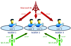
Figure 1: An example of the system model, where user 1, 2, 3, and 4 are moving within the set of locations ${\cal S}=\left\{{1,2,3}\right\}$. The macrocell covers all locations. Each location is covered by a set of Wi-Fi networks, e.g., ${{\cal N}_{1}}=\left\{1\right\}$, ${{\cal N}_{2}}=\left\{1,2\right\}$, ${{\cal N}_{3}}=\left\{2\right\}$.

II-A Two-timescale operations

The operator aims at reducing the total power consumption through the network selection, subchannel allocation, and power allocation. We assume that the network selection is operated in a larger timescale than the subchannel and power allocation. This is because a frequent switch among different networks interrupts the data delivery and incurs a nonnegligible cost (e.g., in the form of energy consumption, quality-of-service degradation, and delays).

We refer every $T$ time slots as a frame, and define the $k$-th frame ($k\in{\mathbb{N}}$) as the time interval that contains a set ${{\cal T}_{k}}\triangleq\left\{{kT,kT+1,\ldots,kT+T-1}\right\}$ of time slots. We assume that:

• the operator determines network selection at the beginning of every frame (large-timescale);

• the operator determines subchannel and power allocation at the beginning of every time slot (small-timescale).

We illustrate such a two-timescale structure in Figure 2.

II-B Frame-based network selection

At time slot $t=kT$, i.e., the beginning of the $k$-th frame, the operator determines the network selection for the $k$-th frame. We denote the network selection by ${\bm{\alpha}}\left(kT\right)=\left(\alpha_{l}\left(kT\right),\forall l\in\mathcal{L}\right)$, where ${\alpha_{l}}\left(kT\right)$ indicates the network that user $l$ is connected to during the $k$-th frame. Let the random variable ${S_{l}}\left(kT\right)\in{\cal S}$ be user $l$’s location during the $k$-th frame, and define ${\bm{S}}\left(kT\right)=\left(S_{l}\left(kT\right),\forall l\in\mathcal{L}\right)$. Since the availabilities of Wi-Fi networks are location-dependent, we have the following constraint for ${\bm{\alpha}}\left(kT\right)$:

$${\alpha_{l}}\left(kT\right)\in{{\cal N}_{{S_{l}}\left(kT\right)}}\cup\left\{0\right\},{\rm{~{}}}\forall l\in\mathcal{L},k=0,1,\ldots,$$ (1)

where selection ${\alpha_{l}}\left(kT\right)=0$ indicates that user $l$ is connected to the macrocell network.

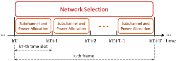
Figure 2: Two-timescale operations: (a) at time $t=kT$, e.g., the beginning of the $k$-th frame, the operator determines the network selection for the $k$-th frame; (b) at time $t\in{\cal T}_{k}$, the operator determines the subchannel and power allocation for time slot $t$.

II-C Macrocell network model

We consider an Orthogonal Frequency Division Multiplexing (OFDM) system for the macrocell network, following the standard model as used in [23, 24].

II-C1 Subchannel allocation

Let ${\cal M}\triangleq\left\{1,2,\ldots,M\right\}$ be the set of subchannels, and denote the subchannel allocation by ${\bm{x}}\left(t\right)=\left(x_{lm}\left(t\right),\forall l\in{\mathcal{L}},m\in{\mathcal{M}}\right)$. Variable $x_{lm}\left(t\right)\in\left\{0,1\right\}$ for all $l$ and $m$: if user $l$ is allocated with subchannel $m$, $x_{lm}\left(t\right)=1$; otherwise, $x_{lm}\left(t\right)=0$. We assume that each subchannel can at most be allocated to one user:

$$\sum\limits_{l=1}^{L}{x_{lm}}\left(t\right)\leq 1,\forall m\in\cal M.\vspace{-0.15cm}$$ (2)

Different from the frame-based network selection ${\bm{\alpha}}\left(kT\right)$, the operator determines the subchannel allocation ${\bm{x}}\left(t\right)$ every time slot. Since the operator can only allocate subchannels to those users who are connected to the cellular network, we have the following constraint for ${\bm{x}}\left(t\right)$:

$${\alpha_{l}\left(t_{T}\right)}{x_{lm}\left(t\right)}=0,\forall l\in{\cal L},m\in{\cal M},t\geq 0.$$ (3)

Here, ${t_{T}}\triangleq{\left\lfloor{\frac{t}{T}}\right\rfloor}T$ is the beginning of the frame that time slot $t$ belongs to, and network selection ${\alpha_{l}\left(t_{T}\right)}$ indicates user $l$’s associated network during the frame.

II-C2 Power allocation

We denote the power allocation by ${\bm{p}}\left(t\right)=\left(p_{lm}\left(t\right),\forall l\in{\mathcal{L}},m\in{\mathcal{M}}\right)$. Variable $p_{lm}\left(t\right)\geq 0$ denotes the power allocated to user $l$ on subchannel $m$. We have the following power budget constraint:

$$\sum\limits_{m=1}^{M}{\sum\limits_{l=1}^{L}{p_{lm}\left(t\right)}}\leq P_{\max}^{C},\forall t\geq 0.$$ (4)

Similar as (3), the operator can only allocate the power to those users who are connected to the cellular network. We have the following constraint for ${\bm{p}}\left(t\right)$:

$${\alpha_{l}\left(t_{T}\right)}{p_{lm}\left(t\right)}=0,\forall l\in{\cal L},m\in{\cal M},t\geq 0.$$ (5)

II-C3 Macrocell transmission rate

We use ${\bm{H}}\left(t\right)=\left(H_{lm}\left(t\right),\forall l\in{\cal L},m\in{\cal M}\right)$ to denote the channel conditions, where $H_{lm}\left(t\right)$ is a random variable that represents the channel condition for user $l$ on subchannel $m$ at time slot $t$. Given the subchannel allocation ${\bm{x}}^{l}\left(t\right)=\left(x_{lm}\left(t\right),\forall m\in{\mathcal{M}}\right)$ and power allocation ${\bm{p}}^{l}\left(t\right)=\left(p_{lm}\left(t\right),\forall m\in{\mathcal{M}}\right)$, the transmission rate of a cellular user $l$ (i.e., ${\alpha_{l}\left(t_{T}\right)}=0$) at time slot $t$ is

$${r_{l}^{C}}\bigl{(}{\bm{x}}^{l}\left(t\right),{\bm{p}}^{l}\left(t\right)\bigr{)}=\!\!\frac{B}{M}\!\sum\limits_{m=1}^{M}{{x_{lm}\left(t\right)}{\log_{2}\left({1\!+\!\frac{{{p_{lm}\left(t\right)}H_{lm}^{2}\left(t\right)}}{{{N_{0}}\frac{B}{M}}{}}}\right)}},$$ (6)

where $B$ is the total bandwidth and $N_{0}$ is the noise power spectral density.

II-C4 Macrocell power consumption

According to [7], the power consumption of the macrocell base station contains two components: the first component is a fixed term that measures the radio frequency (RF) and baseband unit power consumptions; the second component corresponds to the transmission power. Since the first component is fixed, in our model, we focus on minimizing the time average of the second component, which is given by

$$P^{C}\left({{\bm{p}}\left(t\right)}\right)=\kappa\sum\limits_{m=1}^{M}{\sum\limits_{l=1}^{L}{p_{lm}\left(t\right)}}.$$ (7)

Here, parameter $\kappa$ is the scale factor that depends on the power amplifier efficiency and the losses incurred by the antenna feeder, power supply, and cooling [7].

II-D Wi-Fi network model

Let ${\rho_{n}}$ be the number of users associated with Wi-Fi network $n$. We assume that Wi-Fi network $n$’s total transmission rate and power consumption are functions of ${\rho_{n}}$, and we denote them by $R_{n}\left({\rho_{n}}\right)$ and $P_{n}^{W}\left({\rho_{n}}\right)$, respectively. We further assume that $R_{n}\left({\rho_{n}}\right)$ and $P_{n}^{W}\left({\rho_{n}}\right)$ are non-negative bounded functions, i.e., there exist positive constants ${R_{n,\max}}$ and $P_{n,\max}^{W}$ such that

$$0\leq{R_{n}}\left({\rho_{n}}\right)\leq{R_{n,\max}}{\rm~{}and~{}}0\leq P_{n}^{W}\left({\rho_{n}}\right)\leq P_{n,\max}^{W}$$ (8)

for all ${\rho_{n}}=0,1,2,\ldots$.

We allow general functions of $R_{n}\left({\rho_{n}}\right)$ and $P_{n}^{W}\left({\rho_{n}}\right)$ that satisfy (8) in our algorithm design in Sections IV and V. In Section VI, we apply the transmission rate function $R_{n}\left({\rho_{n}}\right)$ defined in [26], and the power consumption function $P_{n}^{W}\left({\rho_{n}}\right)$ defined in [27] for simulation.

II-D1 Wi-Fi transmission rate

Given function $R_{n}\left({\rho_{n}}\right)$ and network selection ${\bm{\alpha}}\left(t_{T}\right)$, we can compute the transmission rate of a Wi-Fi user $l$ (i.e., $\alpha_{l}\left(t_{T}\right)>0$) at time slot $t$ by [28]:

$$r_{l}^{W}\left({{\bm{\alpha}}\left({{t_{T}}}\right)}\right)=\frac{{{R_{\alpha_{l}\left(t_{T}\right)}}\left({\sum\limits_{k=1}^{L}{{{\mathds{1}}_{\left\{{{\alpha_{k}}\left({{t_{T}}}\right)={\alpha_{l}}\left({{t_{T}}}\right)}\right\}}}}}\right)}}{{\sum\limits_{k=1}^{L}{{{\mathds{1}}_{\left\{{\alpha_{k}}\left({{t_{T}}}\right)={\alpha_{l}}\left({{t_{T}}}\right)\right\}}}}}}.$$ (9)

Here, summation ${{\sum\limits_{k=1}^{L}{{{\mathds{1}}_{{\alpha_{k}}\left({{t_{T}}}\right)={\alpha_{l}}\left({{t_{T}}}\right)}}}}}$ returns the number of users in the Wi-Fi network that user $l$ is associated with.

II-D2 Wi-Fi power consumption

Given function $P_{n}^{W}\left({\rho_{n}}\right)$ and network selection ${\bm{\alpha}}\left(t_{T}\right)$, we can compute the power consumption of all Wi-Fi networks as:

$${P^{W}}\left({{\bm{\alpha}}\left({{t_{T}}}\right)}\right)=\sum\limits_{n=1}^{N}{P_{n}^{W}\left({\sum\limits_{l=1}^{L}{{{\mathds{1}}_{\left\{{{\alpha_{l}}\left({{t_{T}}}\right)=n}\right\}}}}}\right)}.$$ (10)

II-E Users’ traffic model

We assume that the users randomly generate traffic, and the traffic generation is not affected by the operator’s operations. We use a random variable $A_{l}\left(t\right)$ to denote the traffic arrival rate of user $l\in{\cal L}$ at time slot $t$, and let ${\bm{A}}\left(t\right)=\left(A_{l}\left(t\right),l\in{\cal L}\right)$. We assume that there exists a positive constant $A_{\max}$ such that

$$0\leq{A_{l}}\left(t\right)\leq{A_{\max}},\forall l\in{\cal L},t\geq 0.$$ (11)

II-F Summary

II-F1 Macrocell $+$ Wi-Fi transmission rate

If a user is associated with the macrocell network, its transmission rate is given by ${{r_{l}^{C}}\left({\bm{x}}^{l}\left(t\right),{\bm{p}}^{l}\left(t\right)\right)}$ in (6); if it is associated with Wi-Fi networks, its transmission rate is given by ${r_{l}^{W}\left({{\bm{\alpha}}\left({{t_{T}}}\right)}\right)}$ in (9). To summarize, user $l$’s transmission rate at time slot $t$ is given by

$${r_{l}}\bigl{(}{{\bm{\alpha}}\left({{t_{T}}}\right)\!,\!{{\bm{x}}^{l}}\left(t\right)\!,\!{{\bm{p}}^{l}}\left(t\right)}\bigr{)}\!=\!\left\{{\begin{array}[]{*{20}{l}}{{r_{l}^{C}}\!\bigl{(}{\bm{x}}^{l}\!\left(t\right)\!,{\bm{p}}^{l}\!\left(t\right)\bigr{)},}&{{\rm if~{}\!}{\alpha_{l}\!\left(t_{T}\!\right)\!=0,}}\\ {r_{l}^{W}\bigl{(}{{\bm{\alpha}}\left({{t_{T}}}\right)}\bigr{)},}&{{\rm otherwise}.}\end{array}}\right.$$ (14)

Because of the power budget constraint (4) in the macrocell network, function ${{r_{l}^{C}}\left({\bm{x}}^{l}\left(t\right),{\bm{p}}^{l}\left(t\right)\right)}$ is upper bounded. Furthermore, since Wi-Fi networks’ total transmission rates are upper bounded as in (8), function $r_{l}^{W}\left({{\bm{\alpha}}\left({{t_{T}}}\right)}\right)$ is also upper bounded. As a result, there exists a positive constant $r_{\max}$ such that

$$0\leq{{r_{l}}\bigl{(}{{\bm{\alpha}}\left({{t_{T}}}\right),{{\bm{x}}^{l}}\left(t\right),{{\bm{p}}^{l}}\left(t\right)}\bigr{)}}\leq{r_{\max}}$$ (15)

for all $l\in{\cal L}$ and ${{\bm{\alpha}}\left({{t_{T}}}\right),{{\bm{x}}^{l}}\left(t\right),{{\bm{p}}^{l}}\left(t\right)}$ satisfying (1), (2), (3), (4), and (5).

II-F2 Macrocell $+$ Wi-Fi power consumption

The operator considers the power consumption in both the macrocell and Wi-Fi networks. The macrocell network’s power consumption is given by $P^{C}\left({{\bm{p}}\left(t\right)}\right)$ in (7), and Wi-Fi networks’ total power consumption is given by $P^{W}\left({\bm{\alpha}}\left(t_{T}\right)\right)$ in (10). Therefore, the operator’s total power consumption at time slot $t$ is given by

$$P\bigl{(}{{\bm{\alpha}}\left(t_{T}\right),{\bm{p}}\left(t\right)}\bigr{)}=P^{C}\left({{\bm{p}}\left(t\right)}\right)+P^{W}\left({\bm{\alpha}}\left(t_{T}\right)\right).$$ (16)

According to the cellular power budget constraint (4) and the bounded Wi-Fi power consumption condition (8), it is easy to find that $P\left({{\bm{\alpha}}\left(t_{T}\right),{\bm{p}}\left(t\right)}\right)$ is bounded:

$$0\leq P\bigl{(}{{\bm{\alpha}}\left(t_{T}\right),{\bm{p}}\left(t\right)}\bigr{)}\leq P_{\max},\forall t\geq 0,$$ (17)

where $P_{\max}\triangleq\kappa P_{\max}^{C}+\sum\limits_{n=1}^{N}{P_{n,\max}^{W}}$.

II-F3 Randomness

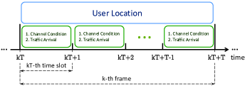
Figure 3: Two-timescale randomness: (a) users’ locations change every frame; (b) channel conditions and users’ traffic arrivals change every time slot.

There are three kinds of randomness in the system:

• Users’ locations ${\bm{S}}\left(kT\right)$, introduced in Section II-B;

• The macrocell network’s channel conditions ${\bm{H}}\left(t\right)$, introduced in Section II-C3;

• Users’ traffic arrivals ${\bm{A}}\left(t\right)$, introduced in Section II-E.

As we assumed in Section II-B, ${\bm{S}}\left(kT\right)$ changes at the beginning of each frame, while ${\bm{H}}\left(t\right)$ and ${\bm{A}}\left(t\right)$ change every time slot. The two-timescale randomnesses is in Figure 3.

III Problem formulation

We assume that each user has a data queue, the length of which denotes the amount of unserved traffic. Let ${\bm{Q}}\left(t\right)=\left(Q_{l}\left(t\right),\forall l\in\cal{L}\right)$ be the queue length vector, where ${Q_{l}}\left(t\right)$ is user $l$’s queue length at time slot $t$. We assume that all queues are initially empty, i.e.,

$${Q_{l}}\left(0\right)=0,{\rm~{}}\forall l\in\cal{L}.\vspace{-0.25cm}$$ (18)

The queue length evolves according to the traffic arrival rate and transmission rate as

$${Q_{l}}\!\left({t\!+\!1}\right)\!\!=\!\!\left[{Q_{l}}\!\left(t\right)\!-\!{{r_{l}}\bigl{(}{{\bm{\alpha}}\!\left({{t_{T}}}\!\right)\!,\!{{\bm{x}}^{l}}\left(t\right)\!,\!{{\bm{p}}^{l}}\!\left(t\right)}\!\bigr{)}}\right]^{+}\!\!+\!{A_{l}}\!\left(t\right),\!\forall l\!\in\!\mathcal{L},t\!\geq\!0.$$ (19)

Here ${\left[x\right]^{+}}=\max\left\{{x,0}\right\}$ is due to the fact that the actual amount of served packets cannot exceed the current queue size.

The objective of the operator is to design an online network selection and resource allocation algorithm that minimizes the expected time average power consumption, while keeping the network stable. This can be formulated as the following optimization problem:

$$\begin{split}&\min{~{}~{}}{\overline{P}}\triangleq\mathop{\limsup}\limits_{K\to\infty}\frac{1}{{KT}}\sum\limits_{t=0}^{KT-1}{{{\mathbb{E}}\left\{{P\left({\bm{\alpha}}\left(t_{T}\right)\right),{\bm{p}}\left(t\right)}\right\}}}\\ &{\rm s.t.~{}~{}}{\overline{Q_{l}}}\triangleq\mathop{\lim\sup}\limits_{K\to\infty}\frac{1}{KT}\sum\limits_{t=0}^{KT-1}{\mathbb{E}{\left\{{Q_{l}}\left(t\right)\right\}}}<\infty{\rm{,~{}}}\forall l\in{\cal L},\\ &{~{}~{}~{}~{}~{}~{}}{\rm constraints~{}~{}(\ref{equ:feasibility}),(\ref{equ:subchannelconstraint}),(\ref{equ:constraintforresource:a}),(\ref{equ:powerbudeget}),(\ref{equ:constraintforresource:b})},\\ &{\rm{var.}}~{}~{}~{}{{\bm{\alpha}}\left(t_{T}\right)},{{\bm{x}}\left(t\right)},{{\bm{p}}\left(t\right)},\forall t\geq 0.\end{split}$$ (20)

Here, ${\overline{Q_{l}}}$ is user $l$’s time average queue length, and constraint ${\overline{Q_{l}}}<\infty$ for all $l\in{\cal L}$ ensures the stability of the network. According to Little’s law, ${\overline{Q_{l}}}$ is proportional to user $l$’s time average traffic delay. We will show that our algorithms guarantee upper bounds for ${\overline{Q_{l}}}$ and thus achieve bounded traffic delay.

IV Network Selection and Resource Allocation Without Prediction

Algorithm 1 Energy-Aware Network Selection and Resource Allocation (ENSRA)

1:  Set $t=0$ and ${\bm{Q}}\left(0\right)={\bm{0}}$;

2:  while $t<t_{end}$ do

3:         if $\mod\left(t,T\right)=0$ $//$ Compute the operations for the frame if $t$ is the beginning time slot of the frame.

4:               Set $k=\frac{t}{T}$ and solve problem (21) to determine ${\bm{\alpha}}\left(kT\right)$, ${\bm{x}}\left(\tau\right)$, ${\bm{p}}\left(\tau\right),\forall\tau\in{\cal T}_{k}$;

5:         end if

6:         Update ${\bm{Q}}\left(t+1\right)$, according to (19);

7:         $t\leftarrow t+1$.

8:  end while

We study the situation where the operator cannot predict the system randomness for the future frames. In Sections IV-A and IV-B, we assume that the operator has the complete information for the channel conditions within the current frame (but not the future frames), and propose ENSRA algorithm to generate a power consumption that can be pushed arbitrarily close to the optimal value of problem (20). In Section IV-C, we analyze the performance of ENSRA. In Section IV-D, we relax the assumption on the complete channel condition information, and discuss the implementation of ENSRA.

IV-A Energy-aware network selection and resource allocation (ENSRA) algorithm

We assume that the operator has the complete information for the channel conditions within the current frame, i.e., at time slot $t=kT$ (the beginning of the $k$-th frame), the operator has the information of ${\bm{H}}\left(\tau\right)$ for all $\tau\in{{{\cal T}_{k}}}$.

$$\begin{split}&\min~{}V\sum\limits_{\tau=kT}^{kT+T-1}{P\bigl{(}{\bm{\alpha}}\left(kT\right),{\bm{p}}\left(\tau\right)\bigr{)}}-\sum\limits_{l=1}^{L}{{Q_{l}}\left({kT}\right)\sum\limits_{\tau=kT}^{kT+T-1}{r_{l}\bigl{(}{{\bm{\alpha}}\left({kT}\right),{{\bm{x}}^{l}}\left(\tau\right),{\bm{p}}^{l}\left(\tau\right)}\bigr{)}}}\\ &{\rm{s.t.}}~{}~{}~{}~{}~{}{\rm constraints~{}~{}(\ref{equ:feasibility}),(\ref{equ:subchannelconstraint}),(\ref{equ:constraintforresource:a}),(\ref{equ:powerbudeget}),(\ref{equ:constraintforresource:b})},\\ &{\rm{var.}}~{}~{}~{}~{}{\bm{\alpha}}\left(kT\right),{\bm{x}}\left(\tau\right),{\bm{p}}\left(\tau\right),\forall\tau\in{\cal T}_{k}.\end{split}$$ (21)

We present ENSRA in Algorithm 1 and illustrate its flowchart in Figure 4. The intuition behind problem (21) in ENSRA can be understood as follows:

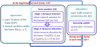
Figure 4: Flowchart of ENSRA algorithm: (a) at the beginning of each frame, the operator determines the network selection and resource allocation for the frame; (b) during each frame, the operator updates users’ traffic queues.

• If user $l$’s queue length $Q_{l}\left(kT\right)$ is small, the operator will focus less on term $-{Q_{l}}\left({kT}\right)\cdot\sum\limits_{\tau=kT}^{kT+T-1}{r_{l}\bigl{(}{{\bm{\alpha}}\left({kT}\right),{{\bm{x}}^{l}}\left(\tau\right),{\bm{p}}^{l}\left(\tau\right)}\bigr{)}}$ and more on term $V\sum\limits_{\tau=kT}^{kT+T-1}{P\bigl{(}{\bm{\alpha}}\left(kT\right),{\bm{p}}\left(\tau\right)\bigr{)}}$ to minimize the objective function in problem (21). This implies that the operator will wait for those good channels or low power cost Wi-Fi networks to serve user $l$. Since $Q_{l}\left(kT\right)$ is small, suspending user $l$’s traffic in several time slots does not heavily increase the average queue length. According to Little’s law, this also does not incur much delay;

• If user $l$’s queue length $Q_{l}\left(kT\right)$ is large, the operator will focus more on term $-{Q_{l}}\left({kT}\right)\cdot\sum\limits_{\tau=kT}^{kT+T-1}{r_{l}\bigl{(}{{\bm{\alpha}}\left({kT}\right),{{\bm{x}}^{l}}\left(\tau\right),{\bm{p}}^{l}\left(\tau\right)}\bigr{)}}$. This implies that there exists a big “pressure” to push the operator to serve user $l$ immediately, even when the user has a poor channel condition or the power needs to serve this user is high. As a result, user $l$’s queue length is reduced and the operator avoids a severe traffic delay.

In summary, by adjusting the control parameter $V>0{}$, the operator can achieve a good tradeoff between the power consumption and the traffic delay under ENSRA.

IV-B Solving problem (21) in ENSRA algorithm

We solve problem (21) in ENSRA in two stages, for the $k$-th frame.

• Stage I (Network Selection): The operator determines the network selection ${\bm{\alpha}}^{*}\left(kT\right)$.

• Stage II (Resource Allocation): Given any network selection ${\bm{\alpha}}\left(kT\right)$, the operator determines the subchannel allocation ${\bm{x}}^{*}\left({\bm{\alpha}}\left(kT\right),\tau\right)$ and power allocation ${\bm{p}}^{*}\left({\bm{\alpha}}\left(kT\right),\tau\right)$ for the macrocell network in each time slot $\tau\in{\cal T}_{k}$.

We solve the two-stage problem by backward induction, and start the analysis from Stage II.

IV-B1 Stage II (Resource Allocation)

Based on the given network selection ${\bm{\alpha}}\left(kT\right)$, we define ${\cal L}_{0}\triangleq\left\{l\in{\cal L}:\alpha_{l}\left(kT\right)=0\right\}$ as the set of users associated with the macrocell network. Due to constraints (3) and (5), we only need to study the subchannel and power allocation for these cellular users. According to (21), we have the following problem in Stage II:

$$\begin{split}&\min~{}V\!\!\!\!\sum\limits_{\tau=kT}^{kT+T-1}{\!\!\!\!P^{C}\!\!\left({\bm{p}}\!\left(\tau\right)\right)}\!-\!\sum\limits_{l\in{\cal L}_{0}}\!{{Q_{l}}\!\left({kT}\right)\!\!\!\!\!\sum\limits_{\tau=kT}^{kT+T-1}\!\!{r_{l}^{C}\!\left({{{\bm{x}}^{l}}\!\left(\tau\right)\!,{\bm{p}}^{l}\!\left(\tau\right)}\right)}}\\ &{\rm{s.t.}}~{}~{}~{}~{}~{}{\rm constraints~{}~{}(\ref{equ:subchannelconstraint}),(\ref{equ:powerbudeget})},\\ &{\rm{var.}}~{}~{}~{}~{}{\bm{x}}^{l}\left(\tau\right),{\bm{p}}^{l}\left(\tau\right),\forall l\in{\cal L}_{0},\tau\in{\cal T}_{k}.\end{split}$$ (22)

It is easy to observe from (22) that the resource allocations for different time slots $\tau\in{\cal T}_{k}$ are fully decoupled. For a particular time slot $\tau\in{\cal T}_{k}$, we expand function ${P^{C}\left({\bm{p}}\left(\tau\right)\right)}$ by (6), function ${r_{l}^{C}\left({{{\bm{x}}^{l}}\left(\tau\right),{\bm{p}}^{l}\left(\tau\right)}\right)}$ by (7), and obtain the following problem:

$$\begin{split}&\max~{}\frac{B}{M}\!\sum\limits_{m=1}^{M}\!{\sum\limits_{l\in{\cal L}_{0}}{{Q_{l}}\!\left(kT\right){x_{lm}}\!\left(\tau\right)\log_{2}\left({1\!+\!\frac{{{p_{lm}}\left(\tau\right)H_{lm}^{2}\left(\tau\right)}}{{{N_{0}}\frac{B}{M}}}}\!\right)}}\\ &{~{}~{}~{}~{}~{}~{}~{}}-V\kappa\sum\limits_{m=1}^{M}{\sum\limits_{l\in{\cal L}_{0}}{{p_{lm}}\left(\tau\right)}}\\ &{\rm{s.t.}}~{}~{}~{}~{}\sum\limits_{m=1}^{M}{\sum\limits_{l\in{\cal L}_{0}}{{p_{lm}}\left(\tau\right)}}\leq{P_{\max}^{C}},\sum\limits_{l\in{\cal L}_{0}}{{x_{lm}}\left(\tau\right)}\leq 1,\forall m,\\ &{\rm{var.}}~{}~{}~{}~{}{x_{lm}}\left(\tau\right)\in\left\{{0,1}\right\},{p_{lm}}\left(\tau\right)\geq 0,\forall l\in{\cal L}_{0},m\in{\cal M}.\end{split}$$ (23)

Problem (23) is similar to the weighted sum throughput maximization problem studied in [23], but with an extra linear power term $-V\kappa\sum\limits_{m=1}^{M}{\sum\limits_{l\in{\cal L}_{0}}{{p_{lm}}\left(\tau\right)}}$ in the objective function. According to [23], the complexity of solving problem (23) is $O\left(LM\right)$. We leave the detailed analysis and solutions to problem (23) in [29].

IV-B2 Stage I (Network Selection)

We use ${\bm{p}}^{*}\bigl{(}{{\bm{\alpha}}\left(kT\right)},\tau\bigr{)}$ and ${\bm{x}}^{*}\bigl{(}{{\bm{\alpha}}\left(kT\right)},\tau\bigr{)}$ to denote the optimal resource allocation at time slot $\tau\in{{\cal T}_{k}}$ under network selection ${{\bm{\alpha}}\left(kT\right)}$. We have obtained ${\bm{p}}^{*}\bigl{(}{{\bm{\alpha}}\left(kT\right)},\tau\bigr{)}$ and ${\bm{x}}^{*}\bigl{(}{{\bm{\alpha}}\left(kT\right)},\tau\bigr{)}$ for all $\tau\in{{\cal T}_{k}}$ in Stage II. Based on (21), the problem in Stage I is formulated as:

$$\begin{split}&\min~{}V\sum\limits_{\tau=kT}^{kT+T-1}{P\Bigl{(}{\bm{\alpha}}\left(kT\right),{\bm{p}}^{*}\big{(}{{\bm{\alpha}}\left(kT\right)},\tau\bigl{)}\Bigr{)}}-\\ &{~{}}\sum\limits_{l=1}^{L}\!{{Q_{l}}\!\left({kT}\right)\!\!\!\!\!\sum\limits_{\tau=kT}^{kT+T-1}\!\!\!\!{r_{l}\Bigl{(}{\!{\bm{\alpha}}\!\left({kT}\right)\!,{{\bm{x}}^{l,*}}\bigr{(}{\bm{\alpha}}\left(kT\right)\!,\!\tau\bigl{)},{\bm{p}}^{l,*}\!\bigr{(}\!{\bm{\alpha}}\!\left(kT\right),\!\tau\!\bigl{)}\!}\Bigr{)}}}\\ &{\rm{s.t.}}~{}~{}~{}{\alpha_{l}}\left(kT\right)\in{{\cal N}_{{S_{l}}\left(kT\right)}}\cup\left\{0\right\},{\rm{~{}}}\forall l\in\mathcal{L}.\end{split}$$ (24)

Problem (24) is a combinatorial optimization problem, and we apply the exhaustive search to pick the optimal network selection ${{\bm{\alpha}}^{*}\left(kT\right)}$.

IV-C Performance analysis of ENSRA

In this section, we prove the performance bounds of ENSRA in terms of the power-delay tradeoff. For ease of exposition, we analyze the performance of ENSRA by assuming that the system randomness is independent and identically distributed (i.i.d.). Notice that with the technique developed in [30], we can obtain similar results under Markovian randomness.

We define the capacity region $\Lambda$ as the closure of the set of arrival vectors that can be stably supported, considering all network selection and resource allocation algorithms. We assume that the mean traffic arrival is strictly interior to $\Lambda$, i.e., there exists an $\eta>0$ such that

$${\mathbb{E}}\left\{{{\bm{A}}\left(t\right)}\right\}+\eta\cdot{\bm{1}}\in\Lambda.$$ (25)

This assumption is commonly used in the network stability literatures [30, 13]. It guarantees that, we can find a network selection and resource allocation algorithm such that each user’s expected transmission rate is greater than its mean traffic arrival rate.

We define the $T$-slot Lyapunov drift ${\Delta}_{T}\left(t\right)$ as

$${\Delta_{T}}\left(t\right)\triangleq{\mathbb{E}}\left\{{\frac{1}{2}\!\sum\limits_{l=1}^{L}{{Q_{l}}{{\left(t+T\right)}^{2}}}\!-\!\frac{1}{2}\sum\limits_{l=1}^{L}{{Q_{l}}{{\left(t\right)}^{2}}}\!\left|{{\bm{Q}}\left(t\right)}\right.}\!\!\right\}.$$ (26)

Intuitively, the $T$-slot Lyapunov drift characterizes the expected change in the quadratic function of the queue length over every $T$ time slots. It will be used to show that ENSRA stabilizes the system and guarantees an upper bound on the time average queue length.

We define the “drift-plus-penalty” term for the $k$-th frame as

$$D_{T}\left(kT\right) \triangleq\Delta_{T}\left(kT\right)+$$

$$V{\mathbb{E}}\left\{\sum\limits_{\tau=kT}^{kT+T-1}{{P\left({\bm{\alpha}}\left(kT\right),{\bm{p}}\left(\tau\right)\right)\left|{{\bm{Q}}\left(kT\right)}\right.}}\right\}.$$ (27)

The “drift-plus-penalty” term captures both the queue variance and the power consumption for the frame. In Lyapunov optimization, we minimize the upper bound of the “drift-plus-penalty” term, which is established in the following lemma (the proofs of all lemmas and theorems can be found in [29]):

Lemma 1

For any values of ${{\bm{Q}}\left(kT\right)}$, ${\bm{\alpha}}\left(kT\right)$, ${\bm{x}}\left(\tau\right)$, and ${\bm{p}}\left(\tau\right)$, $\tau\in{\cal T}_{k}$,

$$D_{T}\left(kT\right)\leq{B_{1}}T+V{\mathbb{E}}\left\{\sum\limits_{\tau=kT}^{kT+T-1}{{P\left({\bm{\alpha}}\left(kT\right),{\bm{p}}\left(\tau\right)\right)\left|{{\bm{Q}}\left(kT\right)}\right.}}\right\}$$

$$+\!{\mathbb{E}}\!\left\{{{\!\sum\limits_{l=1}^{L}{\!\!\sum\limits_{\tau=kT}^{kT+T-1}\!\!\!\!{{{Q_{l}}\!\left(\!\tau\!\right)\!\left(\!{{A_{l}}\!\left(\tau\right)\!-\!{{r_{l}\!\left({{\bm{\alpha}}\!\left({kT}\right)\!,{{\bm{x}}^{l}}\left(\!\tau\right)\!,{\bm{p}}^{l}\left(\!\tau\right)}\!\right)}}}\!\right)}}\!\left|{{\bm{Q}}\!\left(kT\right)}\!\right.}}}\!\right\}\!,$$ (28)

where $B_{1}\triangleq\frac{1}{2}{{L\left({A_{\max}^{2}+r_{\max}^{2}}\right)}}$.

In single-timescale control problems [8], there is no frame structure (i.e., frame size $T=1$), so the upper bound given in Lemma 1 is easy to minimize. However, our work studies two different timescales. Since the queue length ${\bm{Q}}\left(\tau\right)$ correlates users’ transmission rates at time slot $\tau$ with the transmission rates during the time interval $\left[kT,kT+1,\ldots,\tau-1\right]$, it is difficult to directly minimize the upper bound in Lemma 1. Thus, we further relax the upper bound in Lemma 1 in the following lemma.

Lemma 2

For any values of ${{\bm{Q}}\left(kT\right)}$, ${\bm{\alpha}}\left(kT\right)$, ${\bm{x}}\left(\tau\right)$, and ${\bm{p}}\left(\tau\right)$, $\tau\in{\cal T}_{k}$,

$$D_{T}\left(kT\right)\leq{B_{2}}T+V{\mathbb{E}}\left\{\sum\limits_{\tau=kT}^{kT+T-1}{{P\left({\bm{\alpha}}\left(kT\right),{\bm{p}}\left(\tau\right)\right)\left|{{\bm{Q}}\left(kT\right)}\right.}}\right\}$$

$$\!+\!{\mathbb{E}}\!\left\{{{\sum\limits_{l=1}^{L}\!{{Q_{l}}\!\left(kT\right)\!\!\!\!\!\!\sum\limits_{\tau=kT}^{kT+T-1}\!\!\!\!{\!{\left(\!{{A_{l}}\!\left(\tau\right)\!\!-\!\!{{r_{l}\left({\!{\bm{\alpha}}\left({kT}\right)\!,{{\bm{x}}^{l}}\!\left(\!\tau\!\right)\!,{\bm{p}}^{l}\!\left(\tau\right)\!}\right)}}}\right)}}\!\left|{{\bm{Q}}\!\left(kT\right)\!}\right.}}}\!\right\}\!,$$ (29)

where $B_{2}\triangleq\frac{1}{2}{{TL\left({A_{\max}^{2}+r_{\max}^{2}}\right)}}$.

The upper bound in Lemma 2 is independent of ${\bm{Q}}\left(\tau\right)$. As formulated in (21), ENSRA essentially minimizes the right hand side of (29) during every frame. We use $P_{av}^{*}$ to denote the optimal expected time average power consumption of problem (20). The performance of ENSRA is described in the following theorem.

Theorem 1

ENSRA achieves:

$$P_{av}^{\textsf{ENSRA}}\!\triangleq\!\mathop{\limsup}\limits_{K\to\infty}\!\frac{1}{{KT}}\!\!\sum\limits_{t=0}^{KT-1}\!\!{{{\mathbb{E}}\!\left\{\!{P\!\left({\bm{\alpha}}\!\left(t_{T}\right),{\bm{p}}\!\left(t\right)\right)}\!\right\}}}\!\leq\!P_{av}^{*}\!+\!\frac{B_{2}}{V},$$ (30)

$$Q_{av,T}^{\textsf{ENSRA}}\triangleq\mathop{\lim\sup}\limits_{K\to\infty}\frac{1}{K}\sum\limits_{l=1}^{L}{\sum\limits_{k=0}^{K-1}{\mathbb{E}{\left\{{Q_{l}}\left(kT\right)\right\}}}}\leq\frac{{B_{2}+V{P_{\max}}}}{\eta}.$$ (31)

where $B_{2}$ is defined in Lemma 2, $P_{\max}$ is defined in (17), and $\eta$ is defined in (25).

Here, notation $P_{av}^{\textsf{ENSRA}}$ is the expected time average power consumption of ENSRA, and notation $Q_{av,T}^{\textsf{ENSRA}}$ is the expected time average value of user queue length at the beginning of each frame. Based on (31), it is easy to show that the expected time average value of user queue length at each time slot is also upper bounded:

$$Q_{av}^{\textsf{ENSRA}} \triangleq\mathop{\lim\sup}\limits_{K\to\infty}\frac{1}{KT}\sum\limits_{l=1}^{L}{\sum\limits_{t=0}^{KT-1}{\mathbb{E}{\left\{{Q_{l}}\left(t\right)\right\}}}}$$

$$\leq\frac{{B_{2}+V{P_{\max}}}}{\eta}+\!\frac{T-1}{2}LA_{\max}.$$ (32)

Theorem 1 establishes the upper bounds of time average power consumption and queue length (or equivalently, average traffic delay). Theorem 1 implies that, by increasing parameter $V$, the operator can push the power consumption arbitrarily close to the optimal value, i.e., $P_{av}^{*}$, but at the expense of the increase in the average traffic delay.

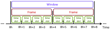
Figure 5: An example of the window structure, where the window size $W=2$, and the frame size $T=4$. The ${h}$-th window contains frames ${\cal T}_{2{h}}=\left\{8{h},8{h}+1,8{h}+2,8{h}+3\right\}$ and ${\cal T}_{2{h}+1}=\left\{8{h}+4,8{h}+5,8{h}+6,8{h}+7\right\}$.

IV-D Implementation of ENSRA: Incomplete Channel Condition Information

In Sections IV-A and IV-B, we assume that the operator has the complete channel condition information for the current frame. In practice, this complete information may not be available, which prevents us from directly solving problem (21) in ENSRA. To implement ENSRA in practice, we revise problem (21) by taking an expectation on the objective function with respect to the channel condition over the $k$-th frame. By minimizing the expected objective function, the operator can determine the network selection for the frame without knowing the channel conditions for the frame. To save space, we provide the detailed algorithm design in [29].

V Network Selection and Resource Allocation With Prediction

We study the situation where the operator can predict the system randomness for the future frames. With the predictive future information, the operator is able to achieve better performance than ENSRA. In Section V-A, we introduce the information prediction model. In Section V-B and V-C, we design and analyze P-ENSRA algorithm. In Section V-D, we design GP-ENSRA algorithm to reduce the computational complexity.

V-A Information prediction model

We consider the structure of the prediction window, where the window size $W$ is the number of frames in a window. Thus, we define the ${h}$-th (${h}\in\left\{{0,1,\ldots}\right\}$) window as the time interval that contains frames ${\cal T}_{{h}W},{\cal T}_{{h}W+1},\ldots,{\cal T}_{{h}W+W-1}$. We use ${\cal W}_{h}\triangleq{{\cal T}_{{h}W}}\cup{{\cal T}_{{h}W+1}}\cup\ldots\cup{{\cal T}_{{h}W+W-1}}$ to define the set of time slots within the ${h}$-th window. Equivalently, we have ${\cal W}_{h}=\left\{{h}WT,{h}WT+1,\ldots,{h}WT+WT-1\right\}$. We illustrate the window structure in Figure 5.

We assume that at time slot $t={h}WT$, i.e., the beginning of the ${h}$-th window, the operator accurately predicts the system randomness for the whole window: (a) ${\bm{S}}\left({h}WT+wT\right),w=0,1,\ldots,W-1$, where ${\bm{S}}\left({h}WT+wT\right)$ denotes users’ locations during frame ${\cal T}_{{h}W+w}$; (b) ${\bm{H}}\left(\tau\right)$, ${\bm{A}}\left(\tau\right),\tau\in{\cal W}_{h}$, where ${\bm{H}}\left(\tau\right)$ and ${\bm{A}}\left(\tau\right)$ denote users’ channel conditions and traffic arrivals at time slot $\tau$, respectively.

At time slot $t={h}WT$, with the predictive information, the operator runs P-ENSRA or GP-ENSRA, and determines the operations for the whole window: (a) ${\bm{\alpha}}\left({h}WT+wT\right),w=0,1,\ldots,W-1$, where ${\bm{\alpha}}\left({h}WT+wT\right)$ denotes the network selection during frame ${\cal T}_{{h}W+w}$; (b) ${\bm{x}}\left(\tau\right),{\bm{p}}\left(\tau\right),\tau\in{\cal W}_{h}$, where ${\bm{x}}\left(\tau\right)$ and ${\bm{p}}\left(\tau\right)$ are the subchannel allocation and power allocation at time slot $\tau$, respectively.

V-B Predictive energy-aware network selection and resource allocation (P-ENSRA) algorithm

$$\begin{split}&\min~{}V\sum\limits_{w=0}^{W-1}{\sum\limits_{\tau=\left({h}W+w\right)T}^{\left({h}W+w+1\right)T-1}{P\bigl{(}{\bm{\alpha}}\left({h}WT+wT\right),{\bm{p}}\left(\tau\right)\bigr{)}}}+\sum\limits_{l=1}^{L}{\sum\limits_{w=0}^{W-1}{{{Q_{l}}\left({{h}WT+wT}\right)}\sum\limits_{\tau=\left({h}W+w\right)T}^{\left({h}W+w+1\right)T-1}{\left(A_{l}\left(\tau\right)+\theta\right)}}}\\ &{~{}~{}~{}~{}~{}~{}}-\sum\limits_{l=1}^{L}{\sum\limits_{w=0}^{W-1}{{{Q_{l}}\left({{h}WT+wT}\right)}\sum\limits_{\tau=\left({h}W+w\right)T}^{\left({h}W+w+1\right)T-1}{r_{l}\bigl{(}{\bm{\alpha}}\left({{h}WT+wT}\right),{{{\bm{x}}^{l}}\left(\tau\right),{\bm{p}}^{l}\left(\tau\right)}\bigr{)}}}}\\ &{\rm{s.t.}}~{}~{}~{}~{}~{}{\rm constraints~{}~{}(\ref{equ:feasibility}),(\ref{equ:subchannelconstraint}),(\ref{equ:constraintforresource:a}),(\ref{equ:powerbudeget}),(\ref{equ:constraintforresource:b})},\\ &{\rm{var.}}~{}~{}~{}~{}{\bm{\alpha}}\left({h}WT+wT\right),w=0,1,\ldots,W-1,{\bm{x}}\left(\tau\right),{\bm{p}}\left(\tau\right),\tau\in{\cal W}_{h}.\end{split}$$ (33)

Algorithm 2 Predictive Energy-Aware Network Selection and Resource Allocation (P-ENSRA)

1:  Set $t=0$ and ${\bm{Q}}\left(0\right)={\bm{0}}$;

2:  while $t<t_{end}$ do

3:         if $\mod\left(t,WT\right)=0$ $//$ Compute the operations for the window if $t$ is the beginning slot of the window.

4:            Set ​${h}\!=\!\frac{t}{WT}$​ and solve problem ​(33)​ to determine ​${\bm{\alpha}}\!\left({h}WT\!+\!wT\right)\!,w\!=\!0,1,\ldots,W\!-\!1,{\bm{x}}\left(\tau\right),{\bm{p}}\left(\tau\right),\!\tau\!\in\!{\cal W}_{h}$;

5:         end if

6:         Update ${\bm{Q}}\left(t+1\right)$, according to (19);

7:         $t\leftarrow t+1$.

8:  end while

We propose P-ENSRA in Algorithm 2. Recall that, the basic idea of ENSRA in Section IV is to minimize the upper bound of the “drift-plus-penalty” term for a frame. As we will see in Section V-C, different from ENSRA, P-ENSRA guarantees a $\theta$-controlled upper bound on the “drift-plus-penalty” term instead of minimizing the “drift-plus-penalty” term for a window. This is because P-ENSRA determines the network selection and resource allocation for several frames (i.e., a window), and it needs to use a novel control parameter $\theta>0$ to balance the queue lengths among different frames. Through introducing $\theta$, we can assign larger weights to the transmission rates of the earlier frames than those of the latter frames within a prediction window. By doing this, we can reduce the time average queue length.

V-C Performance analysis of P-ENSRA

Similar as ENSRA, we characterize the performance of P-ENSRA under the i.i.d. system randomness and assume that the condition (25) is satisfied.

V-C1 Power consumption-delay tradeoff

We define the “drift-plus-penalty” term for the ${h}$-th window as

$$D_{WT}\left({h}WT\right)\triangleq\Delta_{WT}\left({h}WT\right)$$

$$\!\!+\!V\!{\mathbb{E}}\!\left\{\!{{{\sum\limits_{w=0}^{W\!-\!1}{\sum\limits_{\tau=\left({h}W+w\right)T}^{\left({h}W+w+1\right)T\!-\!1}{\!\!\!\!\!P\bigl{(}{\bm{\alpha}}\left({h}WT\!+\!wT\right)\!,{\bm{p}}\left(\tau\right)\bigr{)}}}}\left|{{\bm{Q}}\left({h}WT\right)}\right.}}\!\!\!\right\}.$$ (34)

Next we introduce Lemma 3 and Lemma 4 to show that P-ENSRA guarantees a $\theta$-controlled upper bound on $D_{WT}\left({h}WT\right)$. The introduction of parameter $\theta$ and the $\theta$-controlled upper bound is different from all previous Lyapunov optimization techniques.

Lemma 3

For any values of ${{\bm{Q}}\left({h}WT\right)}$, ${\bm{\alpha}}\left({h}WT+wT\right)$, ${\bm{x}}\left(\tau\right)$, and ${\bm{p}}\left(\tau\right)$, $w=0,1,\ldots,W-1,\tau\in{\cal W}_{h}$, we have (35),

$$D_{WT}\left({h}WT\right)\leq{B_{2}}WT+V{\mathbb{E}}\left\{{{{\sum\limits_{w=0}^{W-1}{\sum\limits_{\tau=\left({h}W+w\right)T}^{\left({h}W+w+1\right)T-1}{P\bigl{(}{\bm{\alpha}}\left({h}WT+wT\right),{\bm{p}}\left(\tau\right)\bigr{)}}}}\left|{{\bm{Q}}\left({h}WT\right)}\right.}}\right\}$$

$$+{\mathbb{E}}\left\{{{\sum\limits_{l=1}^{L}\sum\limits_{w=0}^{W-1}{{Q_{l}}\left({h}WT+wT\right)\sum\limits_{\tau=\left({h}W+w\right)T}^{\left({h}W+w+1\right)T-1}{{\Bigl{(}{{A_{l}}\left(\tau\right)-{{r_{l}\bigl{(}{{\bm{\alpha}}\left({{h}WT+wT}\right),{{\bm{x}}^{l}}\left(\tau\right),{\bm{p}}^{l}\left(\tau\right)}\bigr{)}}}}\Bigr{)}}}\left|{{\bm{Q}}\left({h}WT\right)}\right.}}}\right\},$$ (35)

where $B_{2}$ is the constant defined in Lemma 2.

For any $\theta\in\left({0,\eta}\right]$, we define $P\left(\theta\right)$ as the minimum power consumption required to stabilize the traffic arrival vector ${\mathbb{E}}\left\{{{\bm{A}}\left(t\right)}\right\}+\theta\cdot{\bm{1}}$, considering all network selection and resource allocation algorithms. Naturally, we have the following relation:

$$\mathop{\lim}\limits_{\theta\to 0}{P\left(\theta\right)}=P_{av}^{*}.$$ (36)

Lemma 4

Let ${\bm{\alpha}}^{*}\left({h}WT+wT\right)$, ${\bm{x}}^{*}\left(\tau\right)$, and ${\bm{p}}^{*}\left(\tau\right)$, $w=0,1,\ldots,W-1,\tau\in{\cal W}_{h}$, be the optimal solutions to problem (33). Inequality (37) holds for any $\theta\in\left({0,\eta}\right]$.

$${\mathbb{E}}\!\left\{\!{{\sum\limits_{l=1}^{L}\!\sum\limits_{w=0}^{W-1}{\!{Q_{l}}\!\left({h}WT\!+\!wT\right)\!\!\!\!\!\!\sum\limits_{\tau=\left({h}W+w\right)T}^{\left({h}W+w+1\right)T-1}\!\!\!\!{{\Bigl{(}{\!{A_{l}}\left(\tau\right)\!-\!{{r_{l}\bigl{(}{{{\bm{\alpha}}^{*}}\!\left({{h}WT+wT}\right),{{\bm{x}}^{l,*}}\!\left(\tau\right),{\bm{p}}^{l,*}\!\left(\tau\right)}\bigr{)}}}}\Bigr{)}\!}}\left|{{\bm{Q}}\left({h}WT\right)}\right.}}}\!\!\right\}$$

$$+V{\mathbb{E}}\left\{{{{\sum\limits_{w=0}^{W-1}{\sum\limits_{\tau=\left({h}W+w\right)T}^{\left({h}W+w+1\right)T-1}{P\bigl{(}{\bm{\alpha}}^{*}\left({h}WT+wT\right),{\bm{p}}^{*}\left(\tau\right)\bigr{)}}}}\left|{{\bm{Q}}\left({h}WT\right)}\right.}}\right\}$$

$$\leq-\theta T{\mathbb{E}}\left\{{\sum\limits_{l=1}^{L}{\sum\limits_{w=0}^{W-1}{{{Q_{l}}\left({h}WT+wT\right)}}}\left|{{\bm{Q}}\left({{h}WT}\right)}\right.}\right\}+VWTP\left(\theta\right).$$ (37)

According to Lemma 3 and Lemma 4, P-ENSRA guarantees that

$$D_{WT}\left({h}WT\right)\leq{B_{2}}WT+VWTP\left(\theta\right)$$

$$-\theta T{\mathbb{E}}\left\{{\sum\limits_{l=1}^{L}{\sum\limits_{w=0}^{W-1}{{{Q_{l}}\left({h}WT+wT\right)}}}\left|{{\bm{Q}}\left({{h}WT}\right)}\right.}\right\}.$$ (38)

Here, ${{Q_{l}}\left({h}WT+wT\right)},w=0,1,\ldots,W-1,$ is user $l$’s queue length at the beginning of frame ${\cal T}_{{h}W+w}$ under P-ENSRA. Inequality (38) shows the most important feature of P-ENSRA: it establishes the relation between the “drift-plus-penalty” term and the queue length generated by the algorithm. Based on this, we can prove the upper bound of the average queue length under P-ENSRA (Theorem 2). If we consider other algorithms (e.g., the algorithm that directly minimizes the right hand side of (35) for each window), it is difficult to find a relation similar as (38) and prove the queue length bound. This shows the special design of P-ENSRA.

Based on (38), we show the performance bounds of P-ENSRA. We define $P_{av}^{\textsf{P-ENSRA}}$ as the expected time average power consumption of P-ENSRA, and define $Q_{av,T}^{\textsf{P-ENSRA}}$ as the expected time average value of user queue length at the beginning of each frame under P-ENSRA. The performance of P-ENSRA is described in the following theorem.

Theorem 2

P-ENSRA achieves

$$P_{av}^{\textsf{P-ENSRA}} \triangleq\mathop{\limsup}\limits_{H\to\infty}\frac{1}{{HWT}}\sum\limits_{t=0}^{HWT-1}{{{\mathbb{E}}\left\{{P\left({\bm{\alpha}}\left(t_{T}\right),{\bm{p}}\left(t\right)\right)}\right\}}}$$

$$\leq P\left(\theta\right)+\frac{B_{2}}{V},$$ (39)

$$Q_{av,T}^{\textsf{P-ENSRA}} \triangleq\mathop{\lim\sup}\limits_{H\to\infty}\frac{1}{HW}\sum\limits_{l=1}^{L}{\sum\limits_{{h}=0}^{HW-1}{\mathbb{E}{\left\{{Q_{l}}\left({h}T\right)\right\}}}}$$

$$\leq\frac{{B_{2}+V{P\left(\theta\right)}}}{\theta},$$ (40)

for any $V>0{}$ and $\theta\in\left({0,\eta}\right]$, where $B_{2}$ is defined in Lemma 2.

Based on (40), it is easy to show that the expected time average value of users queue length at each time slot under P-ENSRA is also bounded:

$$Q_{av}^{\textsf{P-ENSRA}} \triangleq\mathop{\lim\sup}\limits_{H\to\infty}\frac{1}{HWT}\sum\limits_{l=1}^{L}{\sum\limits_{t=0}^{HWT-1}{\mathbb{E}{\left\{{Q_{l}}\left(t\right)\right\}}}}$$

$$\leq\frac{{B_{2}+V{P\left(\theta\right)}}}{\theta}+\frac{T-1}{2}LA_{\max},$$ (41)

V-C2 Comparison between ENSRA and P-ENSRA

Comparing Theorem 1 and Theorem 2, we find P-ENSRA achieves similar performance bounds as ENSRA. In particular:

• When $\theta$ approaches $0$, the bound for the power consumption achieved by P-ENSRA equals that of ENSRA in (30). That is,

  $$\mathop{\lim}\limits_{\theta\to 0}\left({P\left(\theta\right)+\frac{B_{2}}{V}}\right)=P_{av}^{*}+\frac{B_{2}}{V};$$ (42)

• When $\theta=\eta$, the average queue length of P-ENSRA satisfies

  $$Q_{av,T}^{\textsf{P-ENSRA}}\leq\frac{{B_{2}+V{P{\left(\eta\right)}}}}{\eta}\leq\frac{{B_{2}+V{P_{\max}}}}{\eta},$$ (43)

  where the right bound is the same as the one specified in (31) for ENSRA.

​​​The reason that the performance bounds of P-ENSRA in (39) and (40) are not better than those of ENSRA is because the performance bounds in (39) and (40) are valid for all delay regimes. As we will observe in Section VI, P-ENSRA cannot outperform ENSRA when the generated delay is restricted to a small value. In this case, the operator has to serve the traffic immediately even if the users’ channel conditions and Wi-Fi availabilities in the future frames are better.

V-D Greedy predictive energy-aware network selection and resource allocation (GP-ENSRA)

In problem (33) the network selections and resource allocations in different frames are tightly coupled by the queue lengths. Such coupling significantly increases the difficulty of directly solving problem (33). Here, we propose a greedy algorithm, GP-ENSRA, which approximately solves problem (33) for each window and significantly reduces the complexity.

Algorithm 3 Greedy Predictive Energy-Aware Network Selection and Resource Allocation (GP-ENSRA)

1:  Set $t=0$ and ${\bm{Q}}\left(0\right)={\bm{0}}$;

2:  while $t<t_{end}$ do

3:         if $\frac{t}{{WT}}\in{\mathbb{N}}$ $//$ Compute the operations for the window if $t$ is the beginning slot of the window.

4:             Set ${h}=\frac{t}{WT}$, $i=0$, and $\bm{\beta}\left({h}WT+wT\right)={\bm{0}}$, $\forall w=0,1,\ldots,W-1$;

5:               while $i<2$ or ${F^{i-1}}-{F^{i}}>\epsilon$ do $//$ Approximately solve problem (33).

6:                     $i\leftarrow i+1$;

7:                     for $w=0$ to $W-1$ do

8:                             Minimize the objective function in problem (33) over $\bm{\beta}\left({h}WT\!+\!wT\right)$ (fix $\bm{\beta}\left({h}WT\!+\!w^{\prime}T\right)$ for all $w^{\prime}\!\neq\!w$);

9:                     Update $\bm{\beta}\left({h}WT+wT\right)$ with the optimal solution obtained in line 8;

10:                     end for

11:                     Denote the value of the objective function in (33) under $\bigl{(}\bm{\beta}\left({h}WT+wT\right),w=0,1,\ldots,W-1\bigr{)}$ by $F^{i}$;

12:               end while

13:               Output vector $\bm{\beta}\left({h}WT+\!wT\right),w\!=\!0,1,\ldots,W\!-\!1,$ as the operations for the window;

14:         end if

15:         Update ${\bm{Q}}\left(t+1\right)$, according to (19);

16:         $t\leftarrow t+1$.

17:  end while

The basic idea of the greedy algorithm is that, instead of globally searching for the optimal solution to problem (33), the operator iteratively updates the operations for different frames within the window. For example, when updating the operations for frame ${\cal T}_{{h}W+w}$, the operator treats the operations for all other frames, i.e., ${\cal T}_{{h}W+w^{\prime}},w^{\prime}\neq w,w^{\prime}=0,1,\ldots,W-1$, as given constants, and minimizes the objective function over the operations for frame ${\cal T}_{{h}W+w}$.

We present GP-ENSRA in Algorithm 3. In order to simplify the description, we use ${{\bm{\beta}}\left({h}WT\!+\!wT\right)}\!=\!\bigl{(}{{\bm{\alpha}}\left({h}WT\!+\!wT\right)},{{\bm{x}}\left(\tau\right)},{{\bm{p}}\left(\tau\right)},\tau\!\in{\cal T}_{{h}W\!+\!w}\bigr{)}$ to represent the operator’s operations (network selection and resource allocation) over frame ${\cal T}_{{h}W+w}$, $w=0,1,\ldots,W-1$. From line 5 to line 12, the operator iteratively updates the operations for all frames within the window. As shown in line 11, we use $F^{i}$ to denote the value of the objective function in (33) under the $i$-th iteration. The condition for ending the iteration (line 5) implies that the decrease from $F^{i-1}$ to $F^{i}$ is no larger than a positive parameter $\epsilon$. Such a condition is guaranteed to be achievable, and we leave the detailed proof in [29]. Briefly speaking, the updating rule (line 8 and line 9) guarantees that $F^{i}$ is always non-increasing in $i$. Furthermore, we can prove that the objective function in (33) is both lower and upper bounded. As a result, it is easy to show that there exists a finite $i$ such that ${F^{i-1}}-{F^{i}}\leq\epsilon$.

The complexity of GP-ENSRA mainly depends on how we solve the problem specified in line 8. In fact, if the initial queue vector of the window ${\bm{Q}}\left({{h}WT}\right)$ satisfies the condition

$${{Q_{l}}\left({{h}WT}\right)}\geq WTr_{\max},\forall l\in{\cal L},$$ (44)

then the problem in line 8 can be solved as problem (21). The condition guarantees that, during the whole window, there are always enough packets in users’ queues to be served. Such a condition is mild in a heavy traffic situation. We leave the complexity analysis of the case without condition (44) as our future work.

VI Simulation

In Section VI-A, we explain the simulation settings. In VI-B, we introduce a heuristic network selection and resource allocation algorithm for comparison, and simulate the power and delay performance of the heuristic algorithm, ENSRA, and GP-ENSRA, respectively.

VI-A Simulation settings

We simulate the problem with $L=10$ users, $1$ macrocell network, $N=10$ Wi-Fi networks, and $S=100$ locations. Each location has a size of $15\times 15~{}{\rm m^{2}}$. We set the time slot length to be $10$ milliseconds, and the frame length to be $1$ second, i.e., the frame size $T=100$. We run each experiment in MATLAB for $5,000$ frames.

VI-A1 Macrocell network

We assume that the macrocell network covers all locations. We consider $M=8$ subchannels, and assume that the channel gain ${H_{lm}}\left(t\right)=\frac{{{\xi_{lm}}\left(t\right)}}{{d_{l}^{1.5}\left(t\right)}}$ follows the Rayleigh fading, where ${\xi_{lm}}\left(t\right)$ follows a Rayleigh distribution [33] and $d_{l}\left(t\right)$ is the distance between user $l$ and the macrocell base station. Distance $d_{l}\left(t\right)$ is computed as follows. We use function $g\left(s\right)$ to denote the distance between the macrocell base station and the users at location $s\in{\cal S}$. In Section II-B, we use $S_{l}\left(kT\right)$ to denote user $l$’s location during the $k$-th frame. Hence, if $t\in{\cal T}_{k}$, distance $d_{l}\left(t\right)$ is determined by $g\left(S_{l}\left(kT\right)\right)$. Table II summarizes other system parameters.

VI-A2 Wi-Fi networks

TABLE II: Simulation Parameters [7, 26, 27]

$P_{\max}^{C}$	$20$ W	$B$	$2.5$ MHz
$N_{0}$	$10^{-7}$ W$/$MHz	$\kappa$	$4.7$
$G$	$800$ b	$T_{b}$	$28$ $\mu$s
$T_{s}$	$100$ $\mu$s	$T_{c}$	$100$ $\mu$s
$E_{b}$	$22.4$ $\mu$J	$E_{s}$	$180$ $\mu$J
$E_{c,j}\left({\rho_{n}}\right)$	$80{\rho_{n}}+100j+80$ $\mu$J

We assume that each Wi-Fi network is randomly distributed spatially, and each Wi-Fi network covers $1\sim 4$ connected locations. We choose the transmission rate function from [26], and define $R_{n}\left({\rho_{n}}\right)$ as:

$${R_{n}}\left({\rho_{n}}\right)=\frac{{{P_{tr}}{P_{s}}G}}{{\left({1-{P_{tr}}}\right){T_{b}}+{P_{tr}}{P_{s}}{T_{s}}+{P_{tr}}\left({1-{P_{s}}}\right){T_{c}}}}.$$ (45)

Here, $G$ is the average payload length, $T_{b}$ is the backoff slot size, $T_{s}$ is the successful transmission slot size, $T_{c}$ is the collision slot size, $P_{tr}=1-{\left({1-\varphi}\right)^{\rho_{n}}}$, $P_{s}=\frac{{\rho_{n}}\varphi{\left({1-\varphi}\right)^{{\rho_{n}}-1}}}{1-{\left({1-\varphi}\right)^{\rho_{n}}}}$, and $\varphi$ is the transmission probability. We choose the power consumption function from [27], and define $P_{n}^{W}\left({\rho_{n}}\right)$ as

$$P_{n}^{W}\left({\rho_{n}}\right)=\frac{{\left({1-{P_{tr}}}\right){E_{b}}+{P_{tr}}{P_{s}}{E_{s}}+\sum\limits_{j=2}^{\rho_{n}}{{P_{c,j}}{E_{c,j}}\left(\rho_{n}\right)}}}{{\left({1-{P_{tr}}}\right){T_{b}}+{P_{tr}}{P_{s}}{T_{s}}+{P_{tr}}\left({1-{P_{s}}}\right){T_{c}}}},$$ (46)

where ${P_{c,j}}={\binom{{\rho_{n}}}{j}}{\varphi^{j}}{\left({1-\varphi}\right)^{{\rho_{n}}-j}}$ and $E_{b}$, $E_{s}$, and $E_{c,j}\left(\rho_{n}\right)$ are the energy consumptions of the backoff slot, successful transmission, and $j$ collided transmissions, respectively. Table II summarizes other system parameters.

VI-A3 Users

We assume that user $l$’s initial location ${S_{l}}\left(0\right)$ is uniformly chosen from set $\cal S$. For all later frames, i.e., $t\in{\cal T}_{k},k>0$, user $l$ moves according to a Markovian process. Similarly, for user $l$’s traffic arrival $A_{l}\left(t\right)$, we generate it based on an ergodic Markov chain. Unless specified otherwise, the mean traffic arrival rate per user is set to be $2$ Mbps.

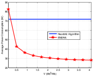
(a) Power vs Parameter $V$.

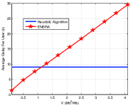
(b) Traffic Delay vs Parameter $V$.

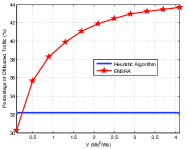
(c) Data Offloading vs Parameter $V$.

Figure 6: Comparison of ENSRA and Heuristic Algorithm.

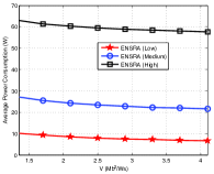
(a) Power Consumption vs Parameter $V$.

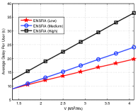
(b) Traffic Delay vs Parameter $V$.

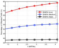
(c) Data Offloading vs Parameter $V$.

Figure 7: ENSRA’s Performance under Low, Medium, and High Workloads.

VI-B Simulation results

VI-B1 Comparison between ENSRA and heuristic algorithm

We compare ENSRA with the following heuristic algorithm.

Heuristic algorithm: At the beginning of each frame, the operator first assigns the users who are only covered by the macrocell network or have $d_{l}\left(t\right)$ smaller than $100{\rm~{}m}$. Then the operator sequentially checks the available Wi-Fi networks for each of the remaining users, and assigns each user to the Wi-Fi network with the lowest number of connected users; at every time slot, the operator determines the resource allocation based on a heuristic method [23].

In Figure 6, we compare ENSRA under different parameter $V$ with the heuristic algorithm. In Figure 6(a), we plot the total power consumption of ENSRA against $V$. We observe that, as $V$ increases, ENSRA’s total power consumption decreases. According to (30), the upper bound of $P_{av}^{\textsf{ENSRA}}$ decreases with the increasing of $V$, which is consistent with our observation here. Figure 6(a) also shows the total power consumption of the heuristic algorithm, which is independent of $V$. We notice that ENSRA consumes less power than the heuristic algorithm for any $V>0.2{}$ ${{{\rm Mb}^{2}}}/{\rm W\cdot s}$.

In Figure 6(b), we plot the average traffic delay per user under ENSRA against $V$. As $V$ increases, the average delay of ENSRA increases, which is consistent with the result in (31). Compared with the heuristic algorithm, ENSRA generates less delay for any $V<1.1{}$ ${{{\rm Mb}^{2}}}/{\rm W\cdot s}$. Figure 6(a) and Figure 6(b) imply that, if the operator chooses $0.2{{{~{}\rm Mb}^{2}}}/{\rm W\cdot s}\leq V\leq 1.1~{}{{{\rm Mb}^{2}}}/{\rm W\cdot s}{}$, ENSRA outperforms the heuristic algorithm in both the power and delay. For example, ENSRA with $V=0.5$ ${{{\rm Mb}^{2}}}/{\rm W\cdot s}{}$ saves $40.8{}$% power and $47.8{}$% delay over the heuristic algorithm.

In Figure 6(c), we plot the percentage of the traffic served in Wi-Fi against $V$. According to (21), a larger $V$ implies that the operator focuses more on the power consumption than the traffic delay, and ENSRA will delay users’ traffic to Wi-Fi networks to reduce the power cost. Hence, in Figure 6(c), the percentage of the traffic served in Wi-Fi increases with $V$.

VI-B2 ENSRA’s performance under different workloads

In Figure 7, We compare ENSRA’s performance under low, medium, and high workloads (the mean traffic arrival rate per user equals $1$ Mbps, $2$ Mbps, and $3$ Mbps, respectively). In Figure 7(a), we observe that ENSRA consumes more power under a higher workload. This is because the minimum power consumption required to stabilize the system increases with the traffic arrival rates. In Figure 7(b), we find that ENSRA generates a larger delay under a higher workload. This is consistent with the reality that users experience severe traffic delay during the peak hours. Figure 7(c) shows that ENSRA offloads a larger percent of traffic to Wi-Fi under a lower workload. The reason is as follows: under the low workload, the operator can offload users’ traffic to the lower cost Wi-Fi networks without causing much delay; while under the high workload, the operator has to fully utilize the cellular and Wi-Fi networks to serve users’ high traffic demand.

VI-B3 Comparison between ENSRA and GP-ENSRA

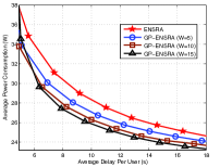
(a) Power-Delay Tradeoff.

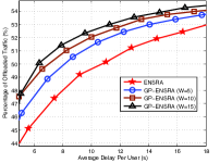
(b) Data Offloading vs Average Delay.

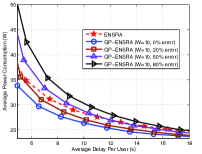
(c) Power-Delay Tradeoff under Prediction Errors.

Figure 8: Comparison of ENSRA and GP-ENSRA.

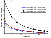
(a) Power vs Parameter $V$.

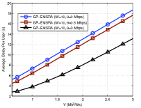
(b) Traffic Delay vs Parameter $V$.

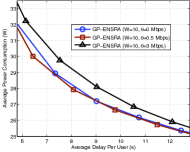
(c) Power-Delay Tradeoff.

Figure 9: Comparison of GP-ENSRA with Different $\theta$.

In Figure 8(a), we plot the average total power consumption against the average traffic delay per user for ENSRA and GP-ENSRA. We obtain these power-delay tradeoff curves by varying $V$. Comparing ENSRA with GP-ENSRA, we observe that when the traffic delay is above $6$ s, GP-ENSRA always generates a smaller power consumption than ENSRA under the same traffic delay. For example, when the generated traffic delay is $8{}$ s, the power consumptions of ENSRA and GP-ENSRA with window size $W=15$ are $30.4{}$ W and $27.4$ W, respectively. Hence, the power saving of GP-ENSRA with $W=15$ over ENSRA is $9.9{}$%. The performance improvement of GP-ENSRA is more obvious in terms of the delay saving. For example, when the operator pursues a power consumption of $26{}$ W, the average traffic delays under ENSRA and GP-ENSRA with window size $W=15$ are $13.9{}$ s and $9.7{}$ s, respectively. This shows that GP-ENSRA with window size $W=15$ saves $30.2{}$% delay over ENSRA. In Figure 8(a), we also observe that the performance improvement increases with the size of the prediction window.

In Figure 8(b), we compare the percentages of the traffic offloaded to Wi-Fi under ENSRA and GP-ENSRA. We plot the percentage of the traffic served in Wi-Fi against the average traffic delay. When generating the same traffic delay, GP-ENSRA offloads a larger percentage of traffic than ENSRA. The reason is that the predictive information helps the operator design a network selection and resource allocation strategy that utilizes Wi-Fi networks more efficiently to reduce the total power consumption.

In Figure 8(c), we investigate the power-delay performance of GP-ENSRA under the prediction errors. For example, GP-ENSRA with $20$% prediction error means that for each information (i.e., users’ locations, channel conditions, and traffic arrivals) of the future frames, with $0.8$ probability the operator accurately predicts its value, while with $0.2$ probability the operator obtains an incorrect value of the information. In Figure 8(c), we plot the average power consumption against the average traffic delay per user for ENSRA and GP-ENSRA with window size $W=10$ under different percentages of the prediction errors. We observe that the power-delay performance of GP-ENSRA declines as the percentage of the prediction errors increases. However, GP-ENSRA with $20\%$ prediction error still achieves a better power-delay tradeoff than the non-predictive algorithm ENSRA, which shows the robustness of GP-ENSRA against the prediction errors.

VI-B4 Influence of Parameter $\theta$ in GP-ENSRA

In Figure 9, we compare GP-ENSRA with window size $W=10$ under different parameter $\theta$. In Figure 9(a), we plot the power consumption against $V$ for GP-ENSRA with different $\theta$, and observe that the power consumption of GP-ENSRA increases with $\theta$. This is because GP-ENSRA is the approximation of P-ENSRA, and the upper bound of the power consumption of P-ENSRA in (39) increases with $\theta$. In Figure 9(b), we plot the average delay against $V$ for GP-ENSRA with different $\theta$. We observe that GP-ENSRA with a large $\theta$ generates a smaller traffic delay. As we explained in Section V-B, with a large $\theta$, the operator assigns large weights to the transmission rates of the earlier frames within the prediction window. The large assigned weights push the operator to serve the traffic in the earlier frames rather than later frames, which eventually decreases the average traffic delay. From Figures 9(a) and 9(b), we conclude that the increase of $\theta$ has two impacts: (i) it increases the power consumption; (ii) it decreases the traffic delay. In Figure 9(c), we plot the power-delay tradeoff for GP-ENSRA with different $\theta$. We find that GP-ENSRA’s power-delay performance first improves with $\theta$ (from $\theta=0{~{}\rm Mbps}$ to $\theta=0.5{~{}\rm Mbps}$) and then declines with $\theta$ (from $\theta=0.5{~{}\rm Mbps}$ to $\theta=3{~{}\rm Mbps}$). This is because, when $0~{}{\rm Mbps}\leq\theta\leq 0.5{~{}}{\rm Mbps}$, the aforementioned impact (ii) plays the dominant role; while when $\theta>0.5{~{}}{\rm Mbps}$, the aforementioned impact (i) plays the dominant role.

VII Conclusion

In this paper, we studied the online network selection and resource allocation problem in the stochastic integrated cellular and Wi-Fi networks. We first proposed the ENSRA algorithm, which can generate a close-to-optimal power consumption at the expense of an increase in the average traffic delay. We then proposed the P-ENSRA algorithm and the GP-ENSRA algorithm by incorporating the prediction of the system randomness into the network selection and resource allocation. Simulation results showed that the future information helps the operator achieve a much better power-delay performance in the large delay regime.

In our future work, we plan to address more challenges related to the power and channel allocation. For example, instead of the continuous power allocation, practical systems usually adopt discrete power control with a limited number of power levels and modulation coding schemes [34]. The discrete power control problem is in general NP-hard. Furthermore, in a practical OFDM system, imperfect carrier synchronization and channel estimation may result in “self-noise” [23]. We intend to incorporate the consideration of the discrete power control and “self-noise” into our algorithm design. Moreover, we want to consider the modified Shannon capacity bounds in [35] to better model the maximum achievable data rate of the macrocell network.

Haoran Yu is a Ph.D. student in the Department of Information Engineering at the Chinese University of Hong Kong (CUHK). He is also a visiting student in the Yale Institute for Network Science (YINS) and the Department of Electrical Engineering at Yale University. His research interests lie in the field of wireless communications and network economics, with current emphasis on mobile data offloading, cellular/Wi-Fi integration, LTE in unlicensed spectrum, and economics of public Wi-Fi networks.

Man Hon Cheung received the B.Eng. and M.Phil. degrees in Information Engineering from the Chinese University of Hong Kong (CUHK) in 2005 and 2007, respectively, and the Ph.D. degree in Electrical and Computer Engineering from the University of British Columbia (UBC) in 2012. Currently, he is a postdoctoral fellow in the Department of Information Engineering in CUHK. He received the IEEE Student Travel Grant for attending IEEE ICC 2009. He was awarded the Graduate Student International Research Mobility Award by UBC, and the Global Scholarship Programme for Research Excellence by CUHK. He serves as a Technical Program Committee member in IEEE ICC, Globecom, and WCNC. His research interests include the design and analysis of wireless network protocols using optimization theory, game theory, and dynamic programming, with current focus on mobile data offloading, mobile crowd sensing, and network economics.

Longbo Huang received his Ph.D. in Electrical Engineering from the University of Southern California (USC) in 2011. He then worked as a postdoctoral researcher in the Electrical Engineering and Computer Sciences department (EECS) at University of California at Berkeley (UC Berkeley) from 2011 to 2012. Since 2012, Dr. Huang has been an assistant professor at the Institute for Interdisciplinary Information Sciences (IIIS) at Tsinghua University, Beijing, China. Dr. Huang was a visiting scholar at the LIDS lab at MIT and at the EECS department at UC Berkeley. He was also a visiting professor at the Chinese University of Hong Kong (CUHK) and at Bell-labs France. Dr. Huang was selected into China’s Youth 1000-talent program in 2013, and received the Google Research Award and the Microsoft Research Asia (MSRA) Collaborative Research Award in 2014. Dr. Huang was selected into the MSRA StarTrack Program in 2015. His paper in ACM MobiHoc 2014 was selected as a Best Paper Finalist. Dr. Huang has served/serves as the TPC Vice Chair for Submissions for WiOpt 2016, and as TPC members for top-tier IEEE and ACM conferences including ACM Sigmetrics/Performance, MobiHoc, INFOCOM, WiOpt, and E-Energy. Dr. Huang’s current research interests are in the areas of learning and optimization for networked systems, mobile networks, data center networking, and smart grid.

Jianwei Huang (S’01-M’06-SM’11-F’16) is an Associate Professor and Director of the Network Communications and Economics Lab (ncel.ie.cuhk.edu.hk), in the Department of Information Engineering at the Chinese University of Hong Kong. He received the Ph.D. degree from Northwestern University in 2005, and worked as a Postdoc Research Associate in Princeton during 2005-2007. He is the co-recipient of 8 international Best Paper Awards, including IEEE Marconi Prize Paper Award in Wireless Communications in 2011. He has co-authored four books: ”Wireless Network Pricing,” ”Monotonic Optimization in Communication and Networking Systems,” ”Cognitive Mobile Virtual Network Operator Games,” and ”Social Cognitive Radio Networks”. He has served as an Associate Editor of IEEE Transactions on Cognitive Communications and Networking, IEEE Transactions on Wireless Communications, and IEEE Journal on Selected Areas in Communications - Cognitive Radio Series. He is the Vice Chair of IEEE ComSoc Cognitive Network Technical Committee and the Past Chair of IEEE ComSoc Multimedia Communications Technical Committee. He is a Fellow of IEEE (Class of 2016) and a Distinguished Lecturer of IEEE Communications Society.

-A Solution to Problem (23)

We first consider the following relaxed problem:

$$\begin{split}&\max~{}-V{\kappa\sum\limits_{m=1}^{M}{\sum\limits_{l\in{\cal L}_{0}}{{p_{lm}}\left(\tau\right)}}}\\ &+\frac{B}{M}\sum\limits_{m=1}^{M}{\sum\limits_{l\in{\cal L}_{0}}{{Q_{l}}\left(kT\right){x_{lm}}\left(\tau\right)\log\left({1+\frac{{{p_{lm}}\left(\tau\right)H_{lm}^{2}\left(\tau\right)}}{{x_{lm}\left(\tau\right)}{{N_{0}}\frac{B}{M}}}}\right)}}\\ &{\rm{s.t.}}~{}~{}~{}~{}~{}\sum\limits_{m=1}^{M}{\sum\limits_{l\in{\cal L}_{0}}{{p_{lm}}\left(\tau\right)}}\leq{P_{\max}^{C}},\sum\limits_{l\in{\cal L}_{0}}{{x_{lm}}\left(\tau\right)}\leq 1,\forall m,\\ &{\rm{var.}}~{}~{}~{}~{}~{}{x_{lm}}\left(\tau\right)\in\left[{0,1}\right],{p_{lm}}\left(\tau\right)\geq 0,\forall l\in{\cal L}_{0},m\in{\cal M}.\end{split}$$ (47)

The differences between problems (47) and (23) are: (1) the noise term ${{{N_{0}}{B}/{M}}}$ is replaced by ${{x_{lm}\left(\tau\right)}{{N_{0}}{B}/{M}}}$; (2) variable ${x_{lm}}\left(\tau\right)\in\left\{{0,1}\right\}$ is replaced by ${x_{lm}}\left(\tau\right)\in\left[{0,1}\right]$. The physical meaning of the relaxation is that we allow the subchannels to be time-shared among users. It is easy to prove that, if ${\bm{x}}^{*}\left({\tau}\right)$ and ${\bm{p}}^{*}\left({\tau}\right)$ are optimal solutions to problem (47) and ${x}^{*}_{lm}\left({\tau}\right)\in\left\{{0,1}\right\}$ for all $l\in{\cal L}_{0},m\in{\cal M}$, ${\bm{x}}^{*}\left({\tau}\right)$ and ${\bm{p}}^{*}\left({\tau}\right)$ are also optimal solutions to problem (23).

Based on [23], problem (47) is convex and satisfies Slater’s condition. We use $\lambda$ to denote the Lagrange multiplier for constraint $\sum\limits_{m=1}^{M}{\sum\limits_{l\in{\cal L}_{0}}{{p_{lm}}\left(\tau\right)}}\leq{P_{\max}^{C}}$, and $\mu_{m}$ to denote the Lagrange multiplier for constraint $\sum\limits_{l\in{\cal L}_{0}}{{x_{lm}}\left(\tau\right)}\leq 1$. The optimal Lagrange multiplier $\lambda^{*}$ is solved by the following problem (see [23] for details):

$${\mathop{\max}\limits_{\lambda\geq 0}\lambda{P_{\max}^{C}}+\sum\limits_{m=1}^{M}{\mu_{m}^{*}\left(\lambda\right)}},$$ (48)

where function ${\mu_{m}^{*}\left(\lambda\right)}$ is given as

$$\mu_{m}^{*}\left(\lambda\right)=\mathop{\max}\limits_{l\in{\cal L}_{0}}{\mu_{lm}}\left(\lambda\right),$$ (49)

and

$${\mu_{lm}}\left(\lambda\right)\triangleq-\left({V\kappa+\lambda}\right)\frac{B}{M}{\left({\frac{{{Q_{l}}\left(kT\right)}}{{V\kappa+\lambda}}-\frac{{{N_{0}}}}{{H_{lm}^{2}\left(\tau\right)}}}\right)^{+}}$$

$$+\frac{B}{M}{Q_{l}}\left(kT\right)\log\left({1+\frac{{H_{lm}^{2}\left(\tau\right)}}{{{N_{0}}}}{{\left({\frac{{{Q_{l}}\left(kT\right)}}{{V\kappa+\lambda}}-\frac{{{N_{0}}}}{{H_{lm}^{2}\left(\tau\right)}}}\right)}^{+}}}\right).$$ (50)

Problem (48) can be optimally solved by using an iterated one dimensional search, e.g., the Golden Section method.

We define ${{\cal A}_{m}}\triangleq\left\{{l\in{\cal L}_{0}:{\mu_{lm}}\left({{\lambda^{*}}}\right)=\mathop{\max}\limits_{l\in{\cal L}_{0}}{\mu_{lm}}\left({{\lambda^{*}}}\right)}\right\}$ for all $m$ under $\lambda^{*}$. We then refer to a subchannel allocation as an extreme point if for all $m\in\cal M$, it satisfies:

• $x_{lm}\left(\tau\right)=0$ if $l\notin{\cal A}_{m}$ and $l\in{\cal L}_{0}$;

• $x_{lm}\left(\tau\right)\in\left\{0,1\right\}$ if $l\in{\cal A}_{m}$;

• $\sum\limits_{l\in{\cal L}_{0}}{x_{lm}\left(\tau\right)}=1$.

Notice that the extreme point implies that the subchannels are not shared among the users and there is exactly one user per subchannel. We then represent such an extreme point by a function $f:{\cal M}\rightarrow\cal L$, where $f\left(m\right)\in{\cal A}_{m}$ indicates the user who is allocated to subchannel $m$. If an extreme point optimizes problem (47), it will also optimize problem (23). Next we discuss the following two cases.

Case a: If there is an extreme point $f$ satisfies:

$$\sum\limits_{m\in\cal M}{\frac{B}{M}{{\left({\frac{{{Q_{l}}\left(kT\right)}}{{V\kappa+{\lambda^{*}}}}-\frac{{{N_{0}}}}{{H_{f\left(m\right)m}^{2}\left(\tau\right)}}}\right)}^{+}}}={P_{\max}^{C}},$$ (51)

then such an extreme point $f$ is optimal to problem (47) [23]. Therefore, it is also optimal to problem (23). Based on $f$, it is easy to obtain ${\bm{x}}^{*}\left(\tau\right)$. Furthermore, we can compute the optimal power allocation ${\bm{p}}^{*}\left(\tau\right)$ by

$${p_{lm}^{*}}\left(\tau\right)=$$

$${x_{lm}^{*}}\left(\tau\right)\frac{B}{M}{\left({\frac{{{Q_{l}}\left(kT\right)}}{{V\kappa+\lambda^{*}}}-\frac{{{N_{0}}}}{{H_{lm}^{2}\left(\tau\right)}}}\right)^{+}},\forall l\in{\cal L}_{0},m\in{\cal M}.$$ (52)

Vectors ${\bm{x}}^{*}\left(\tau\right)$ and ${\bm{p}}^{*}\left(\tau\right)$ are the optimal solutions to problem (23).

Case b: If there is no extreme point $f$ satisfies (51), we need to approximately solve problem (23) by picking the extreme point in a heuristic manner. According to [23], we pick the extreme point $f$, for which $\sum\limits_{m\in{\cal M}_{0}}{\frac{B}{M}{{\left({\frac{{{Q_{l}}\left(kT\right)}}{{V\kappa+{\lambda^{*}}}}-\frac{{{N_{0}}}}{{H_{f\left(m\right)m}^{2}\left(\tau\right)}}}\right)}^{+}}}$ is closest to $P_{max}^{C}$ without exceeding it.

Based on the chosen extreme point $f$, we can quickly determine vector ${\bm{x}}^{*}\left(\tau\right)$. Next we re-optimize the power allocation ${\bm{p}}^{*}\left(\tau\right)$ for the given extreme point $f$. Apparently, we have ${p_{lm}^{*}}\left(\tau\right)=0$ for $l\neq f\left(m\right)$. For the value of ${p_{f\left(m\right)m}^{*}}\left(\tau\right)$, we consider the following problem:

$$\begin{split}&\max~{}\!\frac{B}{M}\!\sum\limits_{m\in\cal M}\!{{Q_{f\left(m\right)}}\!\left(kT\right)\!\log\!\left({1\!+\!\frac{{{p_{f\left(m\right)m}}\left(\tau\right)H_{f\left(m\right)m}^{2}\left(\tau\right)}}{{{N_{0}}\frac{B}{M}}}}\right)}\\ &{~{}~{}~{}~{}~{}~{}~{}~{}}-V\kappa\sum\limits_{m\in\cal M}{{p_{f\left(m\right)m}}\left(\tau\right)}\\ &{\rm{s.t.}}~{}~{}\sum\limits_{m\in\cal M}{{{p_{f\left(m\right)m}}\left(\tau\right)}}\leq{P_{\max}^{C}},\\ &{\rm{var.}}~{}~{}~{}~{}~{}~{}{p_{f\left(m\right)m}}\left(\tau\right)\geq 0,\forall m\in\cal M.\end{split}$$ (53)

Problem (53) is a convex optimization problem, and its optimal solution is described as follows:

• If $\!\sum\limits_{m\in\cal M}\!\!{\frac{B}{M}\!\left(\!{\frac{{{Q_{f\left(m\right)}}\left(kT\right)}}{V\kappa}\!-\!\frac{{{N_{0}}}}{{H_{f\left(m\right)m}^{2}\left(\tau\right)}}}\right)}\leq{P_{\max}^{C}}$, ${p_{f\left(m\right)m}^{*}}\left(\tau\right)$, $m\in\cal M$, is:

  $${p_{f\left(m\right)m}^{*}}\left(\tau\right)=\frac{B}{M}{\left({\frac{{{Q_{f\left(m\right)}}\left(kT\right)}}{{V\kappa}}-\frac{{{N_{0}}}}{{H_{f\left(m\right)m}^{2}\left(\tau\right)}}}\right)^{+}};$$ (54)

• Otherwise, ${p_{f\left(m\right)m}^{*}}\left(\tau\right)$, $m\in\cal M$, is:

  $${p_{f\left(m\right)m}^{*}}\left(\tau\right)=\frac{B}{M}{\left({\frac{{{Q_{f\left(m\right)}}\left(kT\right)}}{{V\kappa}+\vartheta}-\frac{{{N_{0}}}}{{H_{f\left(m\right)m}^{2}\left(\tau\right)}}}\right)^{+}},$$ (55)

  where $\vartheta$ equals ${\sum\limits_{m\in\cal M}{\frac{B}{M}\left({\frac{{{Q_{f\left(m\right)}}\left(kT\right)}}{{V\kappa+\vartheta}}-\frac{{{N_{0}}}}{{H_{f\left(m\right)m}^{2}\left(\tau\right)}}}\right)}^{+}}={P_{\max}^{C}}$.

Vectors ${\bm{x}}^{*}\left(\tau\right)$ and ${\bm{p}}^{*}\left(\tau\right)$ are the solutions to problem (23).

Summarizing Case a and Case b, we solve problem (23).${\rm{~{}}}\Box$

-B Proof of Lemma 1

Recall the queueing dynamics (19):

$${Q_{l}}\left({t+1}\right)= \left[{Q_{l}}\left(t\right)-{{r_{l}}\bigl{(}{{\bm{\alpha}}\left({{t_{T}}}\right),{{\bm{x}}^{l}}\left(t\right),{{\bm{p}}^{l}}\left(t\right)}\bigr{)}}\right]^{+}$$

$$+{A_{l}}\left(t\right),\forall l\in\mathcal{L},t\geq 0.\vspace{-0.2cm}$$ (56)

We then have:

$${Q_{l}}{\left({t+1}\right)^{2}}\leq{Q_{l}}{\left(t\right)^{2}}+{{r_{l}}\bigl{(}{{\bm{\alpha}}\left({{t_{T}}}\right),{{\bm{x}}^{l}}\left(t\right),{{\bm{p}}^{l}}\left(t\right)}\bigr{)}^{2}}+{A_{l}}{\left(t\right)^{2}}$$

$$-2{Q_{l}}\left(t\right){{r_{l}}\bigl{(}{{\bm{\alpha}}\left({{t_{T}}}\right),{{\bm{x}}^{l}}\left(t\right),{{\bm{p}}^{l}}\left(t\right)}\bigr{)}}+2{Q_{l}}\left(t\right){A_{l}}\left(t\right)$$

$$\leq{Q_{l}}{\left(t\right)^{2}}-2{Q_{l}}\left(t\right){{r_{l}}\bigl{(}{{\bm{\alpha}}\left({{t_{T}}}\right),{{\bm{x}}^{l}}\left(t\right),{{\bm{p}}^{l}}\left(t\right)}\bigr{)}}$$

$$+2{Q_{l}}\left(t\right){A_{l}}\left(t\right)+A_{\max}^{2}+r_{\max}^{2}.$$ (57)

Therefore, we compute the upper bound of ${\Delta_{T}}\left(kT\right)$ as (58).

$${\Delta_{T}}\left(kT\right)={\mathbb{E}}\left\{{\frac{1}{2}\sum\limits_{l=1}^{L}{{Q_{l}}{{\left(kT+T\right)}^{2}}}-\frac{1}{2}\sum\limits_{l=1}^{L}{{Q_{l}}{{\left(kT\right)}^{2}}}\left|{{\bm{Q}}\left(kT\right)}\right.}\right\}$$

$$={\mathbb{E}}\left\{\sum\limits_{\tau=kT}^{kT+T-1}{\left({\frac{1}{2}\sum\limits_{l=1}^{L}{{Q_{l}}{{\left(\tau+1\right)}^{2}}}-\frac{1}{2}\sum\limits_{l=1}^{L}{{Q_{l}}{{\left(\tau\right)}^{2}}}}\right)}\left|{{\bm{Q}}\left(kT\right)}\right.\right\}$$

$$\leq{\mathbb{E}}\left\{\sum\limits_{\tau=kT}^{kT+T-1}{\left(B_{1}+{\sum\limits_{l=1}^{L}{\left(-{Q_{l}}\left(\tau\right){{r_{l}}\bigl{(}{{\bm{\alpha}}\left({{kT}}\right),{{\bm{x}}^{l}}\left(\tau\right),{{\bm{p}}^{l}}\left(\tau\right)}\bigr{)}}+{Q_{l}}\left(\tau\right){A_{l}}\left(\tau\right)\right)}}\right)}\left|{{\bm{Q}}\left(kT\right)}\right.\right\}.$$ (58)

Adding $V{\mathbb{E}}\left\{\sum\limits_{\tau=kT}^{kT+T-1}{{P\left({\bm{\alpha}}\left(kT\right),{\bm{p}}\left(\tau\right)\right)\left|{{\bm{Q}}\left(kT\right)}\right.}}\right\}$ to both sides of (58), we prove Lemma 1.${\rm{~{}~{}~{}~{}~{}~{}~{}~{}~{}~{}~{}~{}~{}~{}~{}~{}~{}~{}~{}~{}~{}~{}~{}~{}~{}~{}~{}~{}~{}~{}}}\Box$

-C Proof of Lemma 2

In Lemma 1, we have shown (59).

$$D_{T}\left(kT\right)\leq{B_{1}}T+V{\mathbb{E}}\left\{\sum\limits_{\tau=kT}^{kT+T-1}{{P\left({\bm{\alpha}}\left(kT\right),{\bm{p}}\left(\tau\right)\right)\left|{{\bm{Q}}\left(kT\right)}\right.}}\right\}$$

$$+{\mathbb{E}}\left\{{{\sum\limits_{l=1}^{L}{\sum\limits_{\tau=kT}^{kT+T-1}{{{Q_{l}}\left(\tau\right)\left({{A_{l}}\left(\tau\right)-{{r_{l}\left({{\bm{\alpha}}\left({kT}\right),{{\bm{x}}^{l}}\left(\tau\right),{\bm{p}}^{l}\left(\tau\right)}\right)}}}\right)}}\left|{{\bm{Q}}\left(kT\right)}\right.}}}\right\}.$$ (59)

According to the queueing dynamics (19), we have the following relation for all $l\in{\cal L},\tau\in{\cal T}_{k}$:

$${Q_{l}}\left({kT}\right)\!-\!\left({\tau\!-\!kT}\right){r_{\max}}\leq{Q_{l}}\left(\tau\right)\leq{Q_{l}}\left({kT}\right)\!+\!\left({\tau\!-\!kT}\right){A_{\max}}.$$ (60)

Therefore, we obtain

$${Q_{l}}\left(\tau\right){{A_{l}}\left(\tau\right)}\leq{Q_{l}}\left({kT}\right){{A_{l}}\left(\tau\right)}+\left({\tau-kT}\right){A_{\max}}{{A_{l}}\left(\tau\right)}$$

$$\leq{Q_{l}}\left({kT}\right){{A_{l}}\left(\tau\right)}+\left({\tau-kT}\right){A_{\max}^{2}}.$$ (61)

and

$$-{Q_{l}}\left(\tau\right){{r_{l}\left({{\bm{\alpha}}\left({kT}\right),{{\bm{x}}^{l}}\left(\tau\right),{\bm{p}}^{l}\left(\tau\right)}\right)}}$$

$$\leq-{Q_{l}}\left({kT}\right){{{r_{l}\left({{\bm{\alpha}}\left({kT}\right),{{\bm{x}}^{l}}\left(\tau\right),{\bm{p}}^{l}\left(\tau\right)}\right)}}}$$

$$+\left({\tau-kT}\right){r_{\max}}{{{r_{l}\left({{\bm{\alpha}}\left({kT}\right),{{\bm{x}}^{l}}\left(\tau\right),{\bm{p}}^{l}\left(\tau\right)}\right)}}}$$

$$\leq-{Q_{l}}\left({kT}\right){{{r_{l}\left({{\bm{\alpha}}\left({kT}\right),{{\bm{x}}^{l}}\left(\tau\right),{\bm{p}}^{l}\left(\tau\right)}\right)}}}+\left({\tau-kT}\right){r_{\max}^{2}}.$$ (62)

Based on (59), (61), and (62), we obtain (63).

$$D_{T}\left(kT\right)\leq T\left({T-1}\right){B_{1}}+T{B_{1}}+V{\mathbb{E}}\left\{\sum\limits_{\tau=kT}^{kT+T-1}{{P\left({\bm{\alpha}}\left(kT\right),{\bm{p}}\left(\tau\right)\right)\left|{{\bm{Q}}\left(kT\right)}\right.}}\right\}$$

$$+{\mathbb{E}}\left\{{{\sum\limits_{l=1}^{L}{\sum\limits_{\tau=kT}^{kT+T-1}{{{Q_{l}}\left(kT\right)\left({{A_{l}}\left(\tau\right)-{{r_{l}\left({{\bm{\alpha}}\left({kT}\right),{{\bm{x}}^{l}}\left(\tau\right),{\bm{p}}^{l}\left(\tau\right)}\right)}}}\right)}}\left|{{\bm{Q}}\left(kT\right)}\right.}}}\right\}.$$ (63)

After arrangement, we prove Lemma 2.${\rm{~{}~{}~{}~{}~{}~{}~{}~{}~{}~{}~{}~{}~{}~{}~{}~{}~{}~{}~{}~{}~{}~{}~{}~{}~{}~{}~{}~{}~{}~{}~{}~{}~{}~{}~{}~{}~{}~{}~{}}}\Box$

-D Proof of Theorem 1

Recall the assumption we made in (25), i.e., there exists an $\eta>0$ such that

$${\mathbb{E}}\left\{{{\bm{A}}\left(t\right)}\right\}+\eta\cdot{\bm{1}}\in\Lambda.$$ (64)

According to [13], for any $\varepsilon\in\left[{0,\eta}\right]$, there exists a stationary randomized algorithm that determines network selection and resource allocation independent of queue backlog and yields for frame ${\cal T}_{k}$,

$$\!\sum\limits_{\tau=kT}^{kT+T-1}\!\!\!\left({\mathbb{E}}\left\{{A_{l}\left(\tau\right)}\right\}\!-{\mathbb{E}}\left\{{{r_{l}\!\left({{\bm{\alpha}}\left({kT}\right),{{\bm{x}}^{l}}\!\left(\tau\right)\!,{\bm{p}}^{l}\!\left(\tau\right)}\right)}\!\left|{{\bm{Q}}\left(kT\right)}\!\right.}\right\}\right)\!$$

$$\leq-\varepsilon T,\forall l\in\cal{L},$$ (65)

$${\mathbb{E}}\left\{\sum\limits_{\tau=kT}^{kT+T-1}{{P\left({\bm{\alpha}}\left(kT\right),{\bm{p}}\left(\tau\right)\right)\left|{{\bm{Q}}\left(kT\right)}\right.}}\right\}=P\left(\varepsilon\right)T.$$ (66)

where $P\left(\varepsilon\right)$ is defined in Section V-B.

Next we study $D_{T}\left(kT\right)$ term under ENSRA. Based on Lemma 2, we have (67).

$$D_{T}\left(kT\right)\leq{B_{2}}T+V{\mathbb{E}}\left\{\sum\limits_{\tau=kT}^{kT+T-1}{{P\left({\bm{\alpha}}\left(kT\right),{\bm{p}}\left(\tau\right)\right)\left|{{\bm{Q}}\left(kT\right)}\right.}}\right\}$$

$$+{\mathbb{E}}\left\{{{\sum\limits_{l=1}^{L}{{Q_{l}}\left(kT\right)\sum\limits_{\tau=kT}^{kT+T-1}{{\left({{A_{l}}\left(\tau\right)-{{r_{l}\left({{\bm{\alpha}}\left({kT}\right),{{\bm{x}}^{l}}\left(\tau\right),{\bm{p}}^{l}\left(\tau\right)}\right)}}}\right)}}\left|{{\bm{Q}}\left(kT\right)}\right.}}}\right\}.$$ (67)

Since ENSRA minimizes the right hand side of (67), we compare its value under ENSRA with that under a stationary randomized algorithm. By utilizing (65) and (66), we obtain:

$$D_{T}\left(kT\right)\leq{B_{2}}T+VTP\left(\varepsilon\right)-T\varepsilon{\mathbb{E}}\left\{{{\sum\limits_{l=1}^{L}{{Q_{l}}\left(kT\right)\left|{{\bm{Q}}\left(kT\right)}\right.}}}\right\}.$$ (68)

Taking the expectation of (68) with respect to the distribution of ${\bm{Q}}\left(kT\right)$ and using the law of iterated expectation yields (69).

$$\mathbb{E}\left\{\frac{1}{2}\sum\limits_{l=1}^{L}{\left({{Q_{l}}{{\left({kT+T}\right)}^{2}}-{Q_{l}}{{\left(kT\right)}^{2}}}\right)}+V\sum\limits_{\tau=kT}^{kT+T-1}{P\left({\bm{\alpha}}\left(kT\right),{\bm{p}}\left(\tau\right)\right)}\right\}$$

$$\leq B_{2}T-\varepsilon T{\sum\limits_{l=1}^{L}{\mathbb{E}}\left\{{{Q_{l}}\left(kT\right)}\right\}}+VTP\left(\varepsilon\right).$$ (69)

Summing over time slots $k\in\left\{0,1,\ldots,K-1\right\}$ and dividing by $KT$ yields (70).

$$\frac{1}{{2KT}}\sum\limits_{l=1}^{L}{\mathbb{E}}{\left\{{{{Q_{l}}{{\left(KT\right)}^{2}}-{Q_{l}}{{\left(0\right)}^{2}}}}\right\}}\!\!+\!\!\frac{V}{KT}\sum\limits_{k=0}^{K-1}\sum\limits_{\tau=kT}^{kT+T-1}{\mathbb{E}}{\left\{{P\left({\bm{\alpha}}\left(kT\right),{\bm{p}}\left(\tau\right)\right)}\right\}}$$

$$\leq B_{2}-\frac{\varepsilon}{K}\sum\limits_{k=0}^{K-1}{\sum\limits_{l=1}^{L}{\mathbb{E}}\left\{{{Q_{l}}\left(kT\right)}\right\}}+VP\left(\varepsilon\right).$$ (70)

Part A: Proof of (30)

Because ${\bm{Q}}\left(0\right)={\bm{0}}$ and $Q_{l}\left(kT\right)\geq 0$ for all $l$ and $k$, we have:

$$\frac{V}{KT}\sum\limits_{k=0}^{K-1}\sum\limits_{\tau=kT}^{kT+T-1}{\mathbb{E}}{\left\{{P\left({\bm{\alpha}}\left(kT\right),{\bm{p}}\left(\tau\right)\right)}\right\}}\leq B_{2}+VP\left(\varepsilon\right).$$ (71)

After arrangement, we have

$$\frac{1}{KT}\sum\limits_{k=0}^{K-1}\sum\limits_{\tau=kT}^{kT+T-1}{\mathbb{E}}{\left\{{P\left({\bm{\alpha}}\left(kT\right),{\bm{p}}\left(\tau\right)\right)}\right\}}\leq\frac{B_{2}}{V}+P\left(\varepsilon\right).$$ (72)

Taking limits of the above inequality as $K\to\infty$ yields

$$P_{av}^{\textsf{ENSRA}}\leq\frac{B_{2}}{V}+P\left(\varepsilon\right).$$ (73)

The above inequality holds for all $\varepsilon\in\left[0,\eta\right]$, taking $\varepsilon=0$ yields (30).

Part B: Proof of (31)

Because ${\bm{Q}}\left(0\right)={\bm{0}}$ and $Q_{l}\left(KT\right)\geq 0$ for all $l$, we have the following relation from (70):

$$\frac{\varepsilon}{K}\sum\limits_{k=0}^{K-1}{\sum\limits_{l=1}^{L}{\mathbb{E}}\left\{{{Q_{l}}\left(kT\right)}\right\}}\leq B_{2}+VP\left(\varepsilon\right).$$ (74)

Dividing both sides by $\varepsilon$ and taking limits of the above inequality as $K\to\infty$ yields

$$Q_{av,T}^{\textsf{ENSRA}}\leq\frac{{B_{2}}+VP\left(\varepsilon\right)}{{\varepsilon}}\leq\frac{{B_{2}}+VP_{\max}}{{\varepsilon}}.$$ (75)

The above inequality holds for all $\varepsilon\in\left[0,\eta\right]$, taking $\varepsilon=\eta$ yields (31).

Summarizing Part A and Part B, we complete the proof.${\rm{~{}}}\Box$

-E ENSRA under Incomplete Channel Condition Information

$$\begin{split}&\min~{}V{\mathbb{E}}\left\{{P\left({\bm{\alpha}}\left(kT\right),{\bm{p}}^{*}\left({{\bm{\alpha}}\left(kT\right),\tau}\right)\right)}\right\}-\\ &{~{}~{}~{}~{}~{}~{}~{}}\sum\limits_{l=1}^{L}{{Q_{l}}\left({kT}\right){\mathbb{E}}\left\{{r_{l}\left({{\bm{\alpha}}\left({kT}\right),{{\bm{x}}^{l,*}}\left({\bm{\alpha}}\left(kT\right),\tau\right),{\bm{p}}^{l,*}\left({\bm{\alpha}}\left(kT\right),\tau\right)}\right)}\right\}}\\ &{\rm{s.t.}}~{}~{}~{}~{}~{}~{}~{}~{}~{}~{}{\rm constraint~{}~{}(\ref{equ:feasibility})},\\ &{\rm{variable}}~{}~{}~{}~{}{\bm{\alpha}}\left(kT\right).\end{split}$$ (76)

$$\begin{split}&\min~{}V{P^{C}\left({\bm{p}}\left(t\right)\right)}-\sum\limits_{l\in{\cal L}_{0}}{{Q_{l}}\left({kT}\right){r_{l}^{C}\left({{{\bm{x}}^{l}}\left(t\right),{\bm{p}}^{l}\left(t\right)}\right)}}\\ &{\rm{s.t.}}~{}~{}~{}~{}{\rm constraints~{}~{}(\ref{equ:subchannelconstraint}),(\ref{equ:powerbudeget})},\\ &{\rm{var.}}~{}~{}~{}~{}{\bm{x}}^{l}\left(t\right),{\bm{p}}^{l}\left(t\right),\forall l\in{\cal L}_{0}.\end{split}$$ (77)

Algorithm 4 Revised Energy-Aware Network Selection and Resource Allocation (R-ENSRA)

1:  Set $t=0$ and ${\bm{Q}}\left(0\right)={\bm{0}}$;

2:  while $t<t_{end}$ do

3:         if $\mod\left(t,T\right)=0$ $//$ Compute the network selection for the frame if $t$ is the beginning of the frame.

4:               Set $k=\frac{t}{T}$ and solve problem (76) to determine ${\bm{\alpha}}\left(kT\right)$;

5:         end if

6:         Solve problem (77) to determine ${\bm{x}}\left(t\right),{\bm{p}}\left(t\right)$; $//$ Compute the resource allocation every slot.

7:         Update ${\bm{Q}}\left(t+1\right)$, according to (19);

8:         $t\leftarrow t+1$.

9:  end while

We propose a revised network selection and resource allocation algorithm in Algorithm 4 to tackle the incomplete channel condition. At the beginning time slot of each frame, the operator optimizes an expected function in (76) to determine the network selection. At every time slot, the operator observes the channel condition and solves (77) to determine the resource allocation.

Notice that, we have assumed that the channel conditions ${\bm{H}}\left(t\right)$ are independent and identically distributed over $t$. Therefore, in (76), we only need to optimize the expectation with respect to the channel condition over one time slot instead of the whole frame. The probability distribution of the channel conditions can be approximated by the historical information [9].

-F Proof of Lemma 3

Applying the result of Lemma 2 (the upper bound of the “drift-plus-penalty” term for a frame), we can easily prove Lemma 3 (the upper bound of the “drift-plus-penalty” term for a window).

-G Proof of Lemma 4

According to the objective function in P-ENSRA, P-ENSRA minimizes (78) for each window.

$${\mathbb{E}}\!\left\{\!{{\sum\limits_{l=1}^{L}\!\sum\limits_{w=0}^{W-1}{\!{Q_{l}}\!\left({h}WT\!+\!wT\right)\!\!\!\!\!\!\sum\limits_{\tau=\left({h}W+w\right)T}^{\left({h}W+w+1\right)T-1}\!\!\!\!{{\Bigl{(}{\!{A_{l}}\left(\tau\right)\!+\theta-\!{{r_{l}\bigl{(}{{{\bm{\alpha}}}\!\left({{h}WT+wT}\right),{{\bm{x}}^{l}}\!\left(\tau\right),{\bm{p}}^{l}\!\left(\tau\right)}\bigr{)}}}}\Bigr{)}\!}}\left|{{\bm{Q}}\left({h}WT\right)}\right.}}}\!\!\right\}$$

$$+V{\mathbb{E}}\left\{{{{\sum\limits_{w=0}^{W-1}{\sum\limits_{\tau=\left({h}W+w\right)T}^{\left({h}W+w+1\right)T-1}{P\bigl{(}{\bm{\alpha}}\left({h}WT+wT\right),{\bm{p}}\left(\tau\right)\bigr{)}}}}\left|{{\bm{Q}}\left({h}WT\right)}\right.}}\right\}.$$ (78)

Hence, the value of (78) under P-ENSRA is not greater than that under any randomized algorithm. Recall (65) and (65), we consider the randomized algorithm that satisfies (79) and (80).

$$\sum\limits_{\tau=\left(hW+w\right)T}^{\left(hW+w+1\right)T-1}\left({\mathbb{E}}\left\{{A_{l}\left(\tau\right)}\right\}-{\mathbb{E}}\left\{{{r_{l}\left({{\bm{\alpha}}\left({hWT+wT}\right),{{\bm{x}}^{l}}\left(\tau\right),{\bm{p}}^{l}\left(\tau\right)}\right)}\left|{{\bm{Q}}\left(hWT\right)}\right.}\right\}\right)\leq-\theta T,\forall l\in\cal{L},$$ (79)

$${\mathbb{E}}\left\{\sum\limits_{\tau=\left(hW+w\right)T}^{\left(hW+w+1\right)T-1}{{P\left({\bm{\alpha}}\left(hWT+wT\right),{\bm{p}}\left(\tau\right)\right)\left|{{\bm{Q}}\left(hWT\right)}\right.}}\right\}=P\left(\theta\right)T.$$ (80)

According to these two inequalities, the value of (78) under such a randomized algorithm is not greater than $VTWP\left(\theta\right)$. Therefore, the value of (78) under P-ENSRA is also not greater than $VTWP\left(\theta\right)$. In other words, we have (81) for P-ENSRA.

$${\mathbb{E}}\!\left\{\!{{\sum\limits_{l=1}^{L}\!\sum\limits_{w=0}^{W-1}{\!{Q_{l}}\!\left({h}WT\!+\!wT\right)\!\!\!\!\!\!\sum\limits_{\tau=\left({h}W+w\right)T}^{\left({h}W+w+1\right)T-1}\!\!\!\!{{\Bigl{(}{\!{A_{l}}\left(\tau\right)\!+\theta-\!{{r_{l}\bigl{(}{{{\bm{\alpha}}^{*}}\!\left({{h}WT+wT}\right),{{\bm{x}}^{l,*}}\!\left(\tau\right),{\bm{p}}^{l,*}\!\left(\tau\right)}\bigr{)}}}}\Bigr{)}\!}}\left|{{\bm{Q}}\left({h}WT\right)}\right.}}}\!\!\right\}$$

$$+V{\mathbb{E}}\left\{{{{\sum\limits_{w=0}^{W-1}{\sum\limits_{\tau=\left({h}W+w\right)T}^{\left({h}W+w+1\right)T-1}{P\bigl{(}{\bm{\alpha}}^{*}\left({h}WT+wT\right),{\bm{p}}^{*}\left(\tau\right)\bigr{)}}}}\left|{{\bm{Q}}\left({h}WT\right)}\right.}}\right\}\leq VTWP\left(\theta\right).$$ (81)

Subtracting $\theta T{\mathbb{E}}\left\{{\sum\limits_{l=1}^{L}{\sum\limits_{w=0}^{W-1}{{{Q_{l}}\left({h}WT+wT\right)}}}\left|{{\bm{Q}}\left({{h}WT}\right)}\right.}\right\}$ from both sides, we prove Lemma 4.${\rm{~{}~{}~{}~{}~{}~{}~{}~{}~{}~{}~{}~{}~{}~{}~{}~{}~{}~{}~{}~{}~{}~{}~{}~{}~{}~{}~{}~{}~{}~{}~{}~{}~{}}}\Box$

-H Proof of Theorem 2

According to Lemma 3 and Lemma 4, P-ENSRA guarantees that

$$D_{WT}\left({h}WT\right)\leq{B_{2}}WT$$

$$-\theta T{\mathbb{E}}\left\{{\sum\limits_{l=1}^{L}{\sum\limits_{w=0}^{W-1}{{{Q_{l}}\left({h}WT+wT\right)}}}\left|{{\bm{Q}}\left({{h}WT}\right)}\right.}\right\}+VWTP\left(\theta\right).$$ (82)

Taking the expectation of (82) with respect to the distribution of ${\bm{Q}}\left(hWT\right)$ and using the law of iterated expectation yields

$${\mathbb{E}}\left\{{\frac{1}{2}\sum\limits_{l=1}^{L}{{Q_{l}}{{\left(hWT+WT\right)}^{2}}}-\frac{1}{2}\sum\limits_{l=1}^{L}{{Q_{l}}{{\left(hWT\right)}^{2}}}}\right\}+$$

$$V{\mathbb{E}}\left\{{{{\sum\limits_{w=0}^{W-1}{\sum\limits_{\tau=\left({h}W+w\right)T}^{\left({h}W+w+1\right)T-1}{P\bigl{(}{\bm{\alpha}}\left({h}WT+wT\right),{\bm{p}}\left(\tau\right)\bigr{)}}}}}}\right\}$$

$$\leq{B_{2}}WT+VWTP\left(\theta\right)-\theta T{\mathbb{E}}\left\{{\sum\limits_{l=1}^{L}{\sum\limits_{w=0}^{W-1}{{{Q_{l}}\left({h}WT+wT\right)}}}}\right\}.$$ (83)

Summing over $h\in\left\{0,1,\ldots,H-1\right\}$ and dividing by $HWT$ yields

$$\frac{1}{HWT}{\mathbb{E}}\left\{{\frac{1}{2}\sum\limits_{l=1}^{L}{{Q_{l}}{{\left(HWT\right)}^{2}}}-\frac{1}{2}\sum\limits_{l=1}^{L}{{Q_{l}}{{\left(0\right)}^{2}}}}\right\}+$$

$$\frac{1}{HWT}V{\mathbb{E}}\left\{{{{\sum\limits_{h=0}^{H-1}\!\sum\limits_{w=0}^{W-1}\!{\sum\limits_{\tau=\left({h}W+w\right)T}^{\left({h}W+w+1\right)T-1}{\!\!\!\!P\bigl{(}{\bm{\alpha}}\left({h}WT+wT\right),{\bm{p}}\left(\tau\right)\bigr{)}}}}}}\!\right\}$$

$$\leq{B_{2}}+VP\left(\theta\right)-\frac{\theta}{HW}{\mathbb{E}}\left\{{\sum\limits_{h=0}^{H-1}\sum\limits_{w=0}^{W-1}{\sum\limits_{l=1}^{L}{{{Q_{l}}\left({h}WT+wT\right)}}}}\right\}.$$ (84)

Part A: Proof of (39)

Because ${\bm{Q}}\left(0\right)={\bm{0}}$ and $Q_{l}\left(hWT+wT\right)\geq 0$ for all $l$, $h$, and $w$, we have (85).

$$\frac{1}{HWT}V{\mathbb{E}}\left\{{{{\sum\limits_{h=0}^{H-1}\sum\limits_{w=0}^{W-1}{\sum\limits_{\tau=\left({h}W+w\right)T}^{\left({h}W+w+1\right)T-1}{P\bigl{(}{\bm{\alpha}}\left({h}WT+wT\right),{\bm{p}}\left(\tau\right)\bigr{)}}}}}}\right\}\leq{B_{2}}+VP\left(\theta\right).$$ (85)

After arrangement, we have (86).

$$\frac{1}{HWT}{\mathbb{E}}\left\{{{{\sum\limits_{h=0}^{H-1}\sum\limits_{w=0}^{W-1}{\sum\limits_{\tau=\left({h}W+w\right)T}^{\left({h}W+w+1\right)T-1}{P\bigl{(}{\bm{\alpha}}\left({h}WT+wT\right),{\bm{p}}\left(\tau\right)\bigr{)}}}}}}\right\}\leq\frac{B_{2}}{V}+P\left(\theta\right).$$ (86)

Taking limits of the above inequality as $H\to\infty$ yields (39):

$$P_{av}^{\textsf{P-ENSRA}}\leq\frac{B_{2}}{V}+P\left(\theta\right).$$ (87)

Part B: Proof of (40)

Because ${\bm{Q}}\left(0\right)={\bm{0}}$ and $Q_{l}\left(HWT\right)\geq 0$ for all $l$, we have the following relation from (84):

$$\frac{\theta}{HW}{\mathbb{E}}\left\{{\sum\limits_{h=0}^{H-1}\sum\limits_{w=0}^{W-1}{\sum\limits_{l=1}^{L}{{{Q_{l}}\left({h}WT+wT\right)}}}}\right\}\leq{B_{2}}+VP\left(\theta\right).$$ (88)

Dividing both sides by $\theta$ and taking limits of the above inequality as $H\to\infty$ yields (40):

$$Q_{av,T}^{\textsf{P-ENSRA}}\leq\frac{{B_{2}}+VP\left(\theta\right)}{{\theta}}.$$ (89)

Summarizing Part A and Part B, we complete the proof.${\rm{}}\Box$

-I Iteration Ending Condition in Algorithm 3

Here we prove line 5 in Algorithm 3 is guaranteed to be achievable. We first show the value of the objective function in problem (33) is bounded. Recall problem (33). According to (11), (15), and (17), ${P\bigl{(}{\bm{\alpha}}\left({h}WT+wT\right),{\bm{p}}\left(\tau\right)\bigr{)}}$, ${r_{l}\bigl{(}{\bm{\alpha}}\left({{h}WT+wT}\right),{{{\bm{x}}^{l}}\left(\tau\right),{\bm{p}}^{l}\left(\tau\right)}\bigr{)}}$, and $A_{l}\left(\tau\right)$ are both upper and lower bounded. Furthermore, we have

$$0\leq{{Q_{l}}\left({{h}WT+wT}\right)}\leq\left(hWT+wT\right)A_{\max}.$$ (90)

Therefore, it is easy to show the value of the objective function in problem (33) is also both upper and lower bounded. We denote the bounds as $F_{\max}$ and $F_{\min}$. Since in Algorithm 3, we use $F^{i}$ to denote the objective function’s value in the $i$-th iteration, we have $F_{\min}\leq F^{i}\leq F_{\max}$ for all $i$.

Based on the updating rule (line 8 and line 9), we find $F^{i}$ is always non-increasing in $i$. Hence, if there does not exist a finite $i$ such that ${F^{i-1}}-{F^{i}}\leq\epsilon$, we will have $F^{i-1}-F^{i}>\epsilon$ for $i=3,4,\ldots,3+M$, where $M=\lfloor\frac{F_{\max}-F_{\min}}{\epsilon}\rfloor$. However, this generates $F^{2}-F^{3+M}>\left(M+1\right)\epsilon>F_{\max}-F_{\min}$, which contradicts with the fact that $F_{\min}\leq F^{i}\leq F_{\max}$ for all $i$. Therefore, there exists a finite $i$ such that ${F^{i-1}}-{F^{i}}\leq\epsilon$. In other words, line 5 in Algorithm 3 is guaranteed to be achievable, and we complete the proof.${\rm{~{}~{}~{}~{}~{}~{}~{}~{}~{}~{}~{}~{}~{}~{}~{}~{}~{}~{}~{}~{}~{}~{}~{}~{}}}\Box$

-J GP-ENSRA under Heavy Traffic Region

We study the problem in line 8 of Algorithm 3 under the following condition:

$${{Q_{l}}\left({{h}WT}\right)}\geq WTr_{\max},\forall l\in{\cal L}.$$ (91)

Recall that in Algorithm 3, we use ${{\bm{\beta}}\left({h}WT\!+\!wT\right)}\!=\!\bigl{(}{{\bm{\alpha}}\left({h}WT\!+\!wT\right)},{{\bm{x}}\left(\tau\right)},{{\bm{p}}\left(\tau\right)},\tau\!\in{\cal T}_{{h}W\!+\!w}\bigr{)}$ to represent the operator’s operations over frame ${\cal T}_{{h}W+w}$, $w=0,1,\ldots,W-1$. Based on (33), the problem in line 8 of Algorithm 3 is formulated as (92).

$$\begin{split}&\min~{}V\sum\limits_{w^{\prime}=0}^{W-1}{\sum\limits_{\tau=\left({h}W+w^{\prime}\right)T}^{\left({h}W+w^{\prime}+1\right)T-1}{P\bigl{(}{\bm{\alpha}}\left({h}WT+w^{\prime}T\right),{\bm{p}}\left(\tau\right)\bigr{)}}}\\ &{~{}~{}~{}~{}~{}~{}}-\sum\limits_{l=1}^{L}{\sum\limits_{w^{\prime}=0}^{W-1}{{{Q_{l}}\left({{h}WT+w^{\prime}T}\right)}\sum\limits_{\tau=\left({h}W+w^{\prime}\right)T}^{\left({h}W+w^{\prime}+1\right)T-1}{r_{l}\bigl{(}{\bm{\alpha}}\left({{h}WT+w^{\prime}T}\right),{{{\bm{x}}^{l}}\left(\tau\right),{\bm{p}}^{l}\left(\tau\right)}\bigr{)}}}}\\ &{~{}~{}~{}~{}~{}~{}}+\sum\limits_{l=1}^{L}{\sum\limits_{w^{\prime}=0}^{W-1}{{{Q_{l}}\left({{h}WT+w^{\prime}T}\right)}\sum\limits_{\tau=\left({h}W+w^{\prime}\right)T}^{\left({h}W+w^{\prime}+1\right)T-1}{\left(A_{l}\left(\tau\right)+\theta\right)}}}\\ &{\rm{s.t.}}~{}~{}~{}~{}~{}{\rm constraints~{}~{}(\ref{equ:feasibility}),(\ref{equ:subchannelconstraint}),(\ref{equ:constraintforresource:a}),(\ref{equ:powerbudeget}),(\ref{equ:constraintforresource:b})},\\ &{\rm{var.}}~{}~{}~{}~{}{\bm{\alpha}}\left({h}WT+wT\right),{\bm{x}}\left(\tau\right),{\bm{p}}\left(\tau\right),\tau\in{\cal T}_{hW+w}.\end{split}$$ (92)

The difference between problems (92) and (33) is that, problem (92) only considers the optimization over the operations of one frame, instead of the whole window. In other words, in problem (92), operations ${\bm{\alpha}}\left({h}WT+w^{\prime}T\right)$ and ${\bm{x}}\left(\tau\right),{\bm{p}}\left(\tau\right),\tau\in{\cal T}_{hW+w^{\prime}}$ with $w^{\prime}\neq w,w^{\prime}=0,1,\ldots,W-1$ are treated as given constants.

Removing the terms that are independent of ${\bm{\alpha}}\left({h}WT+wT\right),{\bm{x}}\left(\tau\right),{\bm{p}}\left(\tau\right),\tau\in{\cal T}_{hW+w}$, we can rewrite problem (92) as (93).

$$\begin{split}&\min~{}V{\sum\limits_{\tau=\left({h}W+w\right)T}^{\left({h}W+w+1\right)T-1}{P\bigl{(}{\bm{\alpha}}\left({h}WT+wT\right),{\bm{p}}\left(\tau\right)\bigr{)}}}\\ &{~{}~{}~{}~{}~{}~{}}-\sum\limits_{l=1}^{L}{{{{Q_{l}}\left({{h}WT+wT}\right)}\sum\limits_{\tau=\left({h}W+w\right)T}^{\left({h}W+w+1\right)T-1}{r_{l}\bigl{(}{\bm{\alpha}}\left({{h}WT+wT}\right),{{{\bm{x}}^{l}}\left(\tau\right),{\bm{p}}^{l}\left(\tau\right)}\bigr{)}}}}\\ &{~{}~{}~{}~{}~{}~{}}-\sum\limits_{l=1}^{L}{\sum\limits_{w^{\prime}=w+1}^{W-1}{{{Q_{l}}\left({{h}WT+w^{\prime}T}\right)}\sum\limits_{\tau=\left({h}W+w^{\prime}\right)T}^{\left({h}W+w^{\prime}+1\right)T-1}{r_{l}\bigl{(}{\bm{\alpha}}\left({{h}WT+w^{\prime}T}\right),{{{\bm{x}}^{l}}\left(\tau\right),{\bm{p}}^{l}\left(\tau\right)}\bigr{)}}}}\\ &{~{}~{}~{}~{}~{}~{}}+\sum\limits_{l=1}^{L}{\sum\limits_{w^{\prime}=w+1}^{W-1}{{{Q_{l}}\left({{h}WT+w^{\prime}T}\right)}\sum\limits_{\tau=\left({h}W+w^{\prime}\right)T}^{\left({h}W+w^{\prime}+1\right)T-1}{\left(A_{l}\left(\tau\right)+\theta\right)}}}\\ &{\rm{s.t.}}~{}~{}~{}~{}~{}{\rm constraints~{}~{}(\ref{equ:feasibility}),(\ref{equ:subchannelconstraint}),(\ref{equ:constraintforresource:a}),(\ref{equ:powerbudeget}),(\ref{equ:constraintforresource:b})},\\ &{\rm{var.}}~{}~{}~{}~{}{\bm{\alpha}}\left({h}WT+wT\right),{\bm{x}}\left(\tau\right),{\bm{p}}\left(\tau\right),\tau\in{\cal T}_{hW+w}.\end{split}$$ (93)

According to the queueing dynamics (19) and the fact that ${{Q_{l}}\left({{h}WT}\right)}\geq WTr_{\max},\forall l\in{\cal L}$, we can express ${{Q_{l}}\left({{h}WT+w^{\prime}T}\right)}$ as (94).

$${{Q_{l}}\left({{h}WT+w^{\prime}T}\right)}={{Q_{l}}\left({{h}WT+wT}\right)}+\sum\limits_{w^{\prime\prime}=w+1}^{w^{\prime}-1}\sum\limits_{\tau=\left({h}W+w^{\prime\prime}\right)T}^{\left({h}W+w^{\prime\prime}+1\right)T-1}{\left(A_{l}\left(\tau\right)+\theta\right)}$$

$$-\sum\limits_{w^{\prime\prime}=w+1}^{w^{\prime}-1}\sum\limits_{\tau=\left({h}W+w^{\prime\prime}\right)T}^{\left({h}W+w^{\prime\prime}+1\right)T-1}{{r_{l}\bigl{(}{\bm{\alpha}}\left({{h}WT+w^{\prime\prime}T}\right),{{{\bm{x}}^{l}}\left(\tau\right),{\bm{p}}^{l}\left(\tau\right)}\bigr{)}}}$$

$$+\sum\limits_{\tau=\left({h}W+w\right)T}^{\left({h}W+w+1\right)T-1}{\left(A_{l}\left(\tau\right)+\theta\right)}-\sum\limits_{\tau=\left({h}W+w\right)T}^{\left({h}W+w+1\right)T-1}{{r_{l}\bigl{(}{\bm{\alpha}}\left({{h}WT+wT}\right),{{{\bm{x}}^{l}}\left(\tau\right),{\bm{p}}^{l}\left(\tau\right)}\bigr{)}}}.$$ (94)

Only the last term in (94) depends on the operation during frame ${\cal T}_{hW+w}$. Now we define the following constants:

$$C_{R,l}\triangleq$$

$${\sum\limits_{w^{\prime}=w+1}^{W-1}\!\!\!{\sum\limits_{\tau=\left({h}W+w^{\prime}\right)T}^{\left({h}W+w^{\prime}+1\right)T-1}{\!\!\!\!r_{l}\bigl{(}{\bm{\alpha}}\left({{h}WT+w^{\prime}T}\right),{{{\bm{x}}^{l}}\left(\tau\right),{\bm{p}}^{l}\left(\tau\right)}\bigr{)}}}},$$ (95)

$$C_{A,l}\triangleq{\sum\limits_{w^{\prime}=w+1}^{W-1}{\sum\limits_{\tau=\left({h}W+w^{\prime}\right)T}^{\left({h}W+w^{\prime}+1\right)T-1}{\left(A_{l}\left(\tau\right)+\theta\right)}}}.$$ (96)

Then we can further rewrite problem (93) as (97).

$$\begin{split}&\min~{}V{\sum\limits_{\tau=\left({h}W+w\right)T}^{\left({h}W+w+1\right)T-1}{P\bigl{(}{\bm{\alpha}}\left({h}WT+wT\right),{\bm{p}}\left(\tau\right)\bigr{)}}}\\ &{~{}~{}~{}~{}~{}~{}}-\sum\limits_{l=1}^{L}{{\left({{Q_{l}}\left({{h}WT+wT}\right)}-C_{R,l}+C_{A,l}\right)\sum\limits_{\tau=\left({h}W+w\right)T}^{\left({h}W+w+1\right)T-1}{r_{l}\bigl{(}{\bm{\alpha}}\left({{h}WT+wT}\right),{{{\bm{x}}^{l}}\left(\tau\right),{\bm{p}}^{l}\left(\tau\right)}\bigr{)}}}}\\ &{\rm{s.t.}}~{}~{}~{}~{}~{}{\rm constraints~{}~{}(\ref{equ:feasibility}),(\ref{equ:subchannelconstraint}),(\ref{equ:constraintforresource:a}),(\ref{equ:powerbudeget}),(\ref{equ:constraintforresource:b})},\\ &{\rm{var.}}~{}~{}~{}~{}{\bm{\alpha}}\left({h}WT+wT\right),{\bm{x}}\left(\tau\right),{\bm{p}}\left(\tau\right),\tau\in{\cal T}_{hW+w}.\end{split}$$ (97)

Comparing problem (97) with problem (21), we find they are essentially the same optimization problems. In problem (97), we modify the queue backlog term by constants $C_{R,l}$ and $C_{A,l}$, which are related to the future transmission rates and traffic arrivals. Now, we have shown that, if we have ${{Q_{l}}\left({{h}WT}\right)}\geq WTr_{\max},\forall l\in{\cal L}$, the problem in line 8 can be solved as problem (21).${\rm{~{}~{}~{}~{}~{}~{}~{}~{}~{}~{}~{}~{}~{}~{}~{}~{}~{}~{}~{}~{}~{}~{}~{}~{}~{}~{}~{}~{}~{}~{}~{}~{}~{}~{}~{}~{}~{}~{}~{}~{}~{}~{}~{}~{}~{}~{}~{}~{}~{}~{}~{}~{}~{}~{}}}\Box$

References

- [1] H. Yu, M. H. Cheung, L. Huang, and J. Huang, “Predictive delay-aware network selection in data offloading,” in Proc. of IEEE GLOBECOM, Austin, TX, December 2014, pp. 1376–1381.
- [2] A. Fehske, G. Fettweis, J. Malmodin, and G. Biczók, “The global footprint of mobile communications: The ecological and economic perspective,” IEEE Communications Magazine, vol. 49, no. 8, pp. 55–62, August 2011.
- [3] E. Oh, B. Krishnamachari, X. Liu, and Z. Niu, “Toward dynamic energy-efficient operation of cellular network infrastructure,” IEEE Communications Magazine, vol. 49, no. 6, pp. 56–61, June 2011.
- [4] M. Ismail, W. Zhuang, E. Serpedin, and K. Qaraqe, “A survey on green mobile networking: from the perspectives of network operators and mobile users,” IEEE Communications Surveys & Tutorials, vol. 17, no. 3, pp. 1535–1556, August 2015.
- [5] J. B. Rao and A. O. Fapojuwo, “A survey of energy efficient resource management techniques for multicell cellular networks,” IEEE Communications Surveys & Tutorials, vol. 16, no. 1, pp. 154–180, First Quarter 2014.
- [6] M. Ismail and W. Zhuang, “Network cooperation for energy saving in green radio communications,” IEEE Wireless Communications, vol. 18, no. 5, pp. 76–81, October 2011.
- [7] G. Auer, V. Giannini, C. Desset, I. Godor, P. Skillermark, M. Olsson, M. A. Imran, D. Sabella, M. J. Gonzalez, O. Blume, and A. Fehske, “How much energy is needed to run a wireless network?” IEEE Wireless Communications, vol. 18, no. 5, pp. 40–49, October 2011.
- [8] M. J. Neely, “Energy optimal control for time-varying wireless networks,” IEEE Transactions on Information Theory, vol. 52, no. 7, pp. 2915–2934, July 2006.
- [9] Y. Yao, L. Huang, A. Sharma, L. Golubchik, and M. J. Neely, “Data centers power reduction: A two time scale approach for delay tolerant workloads,” in Proc. of IEEE INFOCOM, Orlando, FL, March 2012, pp. 1431–1439.
- [10] A. J. Nicholson and B. D. Noble, “Breadcrumbs: forecasting mobile connectivity,” in Proc. of ACM MobiCom, San Francisco, CA, September 2008, pp. 46–57.
- [11] U. Paul, A. P. Subramanian, M. M. Buddhikot, and S. R. Das, “Understanding traffic dynamics in cellular data networks,” in Proc. of IEEE INFOCOM, Shanghai, China, April 2011, pp. 882–890.
- [12] M. K. Ozdemir and H. Arslan, “Channel estimation for wireless OFDM systems,” IEEE Communications Surveys & Tutorials, vol. 9, no. 2, pp. 18–48, 2007.
- [13] M. J. Neely, Stochastic Network Optimization With Application to Communication and Queueing Systems. Morgan & Claypool Publishers, 2010.
- [14] L. Venturino, A. Zappone, C. Risi, and S. Buzzi, “Energy-efficient scheduling and power allocation in downlink OFDMA networks with base station coordination,” IEEE Transactions on Wireless Communications, vol. 14, no. 1, pp. 1–14, January 2015.
- [15] C. Xiong, G. Y. Li, S. Zhang, Y. Chen, and S. Xu, “Energy-efficient resource allocation in OFDMA networks,” IEEE Transactions on Communications, vol. 60, no. 12, pp. 3767–3778, December 2012.
- [16] F. Meshkati, H. V. Poor, S. C. Schwartz, and R. V. Balan, “Energy-efficient resource allocation in wireless networks with quality-of-service constraints,” IEEE Transactions on Communications, vol. 57, no. 11, pp. 3406–3414, November 2009.
- [17] M. J. Neely, “Optimal energy and delay tradeoffs for multiuser wireless downlinks,” IEEE Transactions on Information Theory, vol. 53, no. 9, pp. 3095–3113, September 2007.
- [18] Y. Li, M. Sheng, Y. Shi, X. Ma, and W. Jiao, “Energy efficiency and delay tradeoff for time-varying and interference-free wireless networks,” IEEE Transactions on Wireless Communications, vol. 13, no. 11, pp. 5921–5931, November 2014.
- [19] Y. Li, M. Sheng, C.-X. Wang, X. Wang, Y. Shi, and J. Li, “Throughput–delay tradeoff in interference-free wireless networks with guaranteed energy efficiency,” IEEE Transactions on Wireless Communications, vol. 14, no. 3, pp. 1608–1621, March 2015.
- [20] S. Lakshminarayana, M. Assaad, and M. Debbah, “Transmit power minimization in small cell networks under time average QoS constraints,” IEEE Journal on Selected Areas in Communications, 2015.
- [21] http://www.fiercewireless.com/press-releases/12-billion-customer-connections-made-nearly-30000-att-wi-fi-hot-spots-2011.
- [22] DOCOMO, “Docomo 5G white paper,” Tech. Rep., July 2014.
- [23] J. Huang, V. G. Subramanian, R. Agrawal, and R. A. Berry, “Downlink scheduling and resource allocation for OFDM systems,” IEEE Transactions on Wireless Communications, vol. 8, no. 1, pp. 288–296, January 2009.
- [24] Z. Shen, J. G. Andrews, and B. L. Evans, “Adaptive resource allocation in multiuser OFDM systems with proportional rate constraints,” IEEE Transactions on Wireless Communications, vol. 4, no. 6, pp. 2726–2737, November 2005.
- [25] E. Oh, K. Son, and B. Krishnamachari, “Dynamic base station switching-on/off strategies for green cellular networks,” IEEE Transactions on Wireless Communications, vol. 12, no. 5, pp. 2126–2136, May 2013.
- [26] G. Bianchi, “Performance analysis of the IEEE 802.11 distributed coordination function,” IEEE Journal on Selected Areas in Communications, vol. 18, no. 3, pp. 535–547, March 2000.
- [27] B. H. Jung, H. Jin, and D. K. Sung, “Adaptive transmission power control and rate selection scheme for maximizing energy efficiency of IEEE 802.11 stations,” in Proc. of IEEE International Symposium on Personal Indoor and Mobile Radio Communications (PIMRC), September 2012, pp. 266–271.
- [28] M. H. Cheung, R. Southwell, and J. Huang, “Congestion-aware network selection and data offloading,” in Proc. of IEEE CISS, Princeton, NJ, March 2014, pp. 1–6.
- [29] H. Yu, M. H. Cheung, L. Huang, and J. Huang, “Power-delay tradeoff with predictive scheduling in integrated cellular and Wi-Fi networks,” arXiv Tech Report arXiv:1512.06428, 2015.
- [30] L. Huang and M. J. Neely, “Max-weight achieves the exact utility-delay tradeoff under markov dynamics,” arXiv preprint arXiv:1008.0200, 2010.
- [31] L. Huang, S. Zhang, M. Chen, and X. Liu, “When backpressure meets predictive scheduling,” in Proc. of ACM MobiHoc, Philadelphia, PA, August 2014.
- [32] T. S. Rappaport, Wireless communications: Principles and practice. New Jersey: Prentice Hall, 1996.
- [33] V. Gajić, J. Huang, and B. Rimoldi, “Competition of wireless providers for atomic users,” IEEE/ACM Transactions on Networking (TON), vol. 22, no. 2, pp. 512–525, April 2014.
- [34] S. Li, Z. Shao, and J. Huang, “Arm: Anonymous rating mechanism for discrete power control,” in Proc. of IEEE WiOpt, Mumbai, India, May 2015.
- [35] P. Mogensen, W. Na, I. Z. Kovács, F. Frederiksen, A. Pokhariyal, K. Pedersen, T. Kolding, K. Hugl, and M. Kuusela, “LTE capacity compared to the Shannon bound,” in Proc. of IEEE Vehicular Technology Conference, Dublin, Ireland, April 2007, pp. 1234–1238.