A New Calibrated Sunspot Group Series Since 1749: Statistics of Active Day Fractions

1 Introduction

Solar activity regularly changes in the course of the 11-year Schwabe cycle, on top of which it shows also slower secular variability (see, e.g., a review by Hathaway, 2015). This is often quantified using the sunspot number series, which covers, with different levels of data quality, the period since 1610 starting with the first telescopic observations. It is generally accepted (Usoskin, 2013; Hathaway, 2015) that solar activity varies between very low activity, called grand minima, such as the Maunder minimum during 1645 – 1715 (Eddy, 1976; Usoskin et al., 2015) and grand maxima such as the recent period of high activity in the second half of the 20th century called the Modern Grand Maximum (Solanki et al., 2004).

The first attempt to produce a homogeneous sunspot-number series was made by R. Wolf in Zurich in the late 19th century, who produced the famous Wolf (sometimes also called Zurich) sunspot number series. That effort was continued by his successors in Zurich and finally culminated at the Royal Observatory of Belgium as the International sunspot number series (Clette et al., 2014). This series uses the counting method introduced by R. Wolf where the relative sunspot number [$R$] is calculated, for a given observer, as

$$R_{\rm W}=k_{\rm W}\times(10\times G+S),\ilabel{Eq:Rw}$$ (1)

where $k_{\rm W}$ is the correction factor of an individual observer, and $G$ and $S$ are the numbers of sunspot groups and sunspots, respectively, as reported by this observer for a particular day. Unfortunately, the raw data for this series, somewhat subjectively compiled by primary persons starting from R. Wolf, are not available in digital form, making it impossible to revisit except of simple corrections.

A slightly different approach was proposed by Hoyt, Schatten, and Nesmes-Ribes (1994), who used only the number of sunspot groups and ignored the number of individual spots on the disc because their number is less robustly determined. They formed the group sunspot number series $Rg$, where a daily value for each observer was defined as

$$Rg=12.08\times k_{g}\times G.$$ (2)

Here $G$ has the same meaning as in Equation (Eq:Rw), $k_{g}$ may be in general different from $k_{W}$, and 12.08 is a scaling coefficient to match the average values of $Rg$ and the Wolf sunspot number over the interval 1874 – 1976. The original data set used by Wolf was greatly updated, nearly doubling the number of daily sunspot records (Hoyt and Schatten, 1992; Ribes and Nesme-Ribes, 1993; Hoyt and Schatten, 1995a; Hoyt and Schatten, 1995b; Hoyt and Schatten, 1996) culminating in the release of a full sunspot group observation database (referred to as HS98 henceforth Hoyt and Schatten, 1998). HS98 provided a comprehensive database of daily values of $G$ for all the available observers along with the ascribed correction factors. This HS98 database forms a basis for further studies. Newly recovered data are being added to it continuously, along with corrections of erroneous data (e.g., Arlt, 2008; Vaquero and Vázquez, 2009; Vaquero et al., 2011; Arlt et al., 2013; Vaquero and Trigo, 2014; Neuhäuser et al., 2015). Thus, the database of values of $G$ and $S$ exists and is kept up-to-date. However, a major problem lies in the individual correction factors [$k$] (which may be different for different series) for the observers. Since the sunspot number series is a composite series based on observations of the Sun by a large number of individual observers with instruments of different quality and different techniques, it is always a problem to produce a homogeneous series which requires an inter-calibration of the observers (Clette et al., 2014). The standard way to “calibrate” observers to each other is based on a daisy chain of linear regressions (or even linear proportionality) between observers using periods when they overlap. The main disadvantage of this method is that it is possible for errors to propagate and become accumulated over time using “multi-store” regressions (a correction factor [$k$] is obtained by regression with a segment of other data, which has been calibrated by a regression with yet another segment, etc.). For example, if one observer is erroneously assessed, this error will be transferred to all other observers linked to that one. The regression is typically based on daily values (Hoyt and Schatten, 1998), but in in some cases (Svalgaard and Schatten, 2015 referred to as SS15 henceforth) a proportionality between heavily smoothed (annual) values is used which, may lead to a serious bias as shown in Section Sec:nonlin.

Several potential errors in the assessment of observers” quality have been suggested recently, leading to discontinuities such as: the Waldmeier discontinuity in the Wolf and International sunspot number (Clette et al., 2014; Lockwood, Owens, and Barnard, 2014) in the 1940s, related to a change in the sunspot counting algorithm at the Zurich observatory; a jump between observations by Wolf and by Wolfer in the 1880s (Clette et al., 2014); and a discontinuity between Schwabe and Wolf data in 1848 (Leussu et al., 2013). Thus, a need for a revision of the sunspot series by re-calibrating individual observers has become clear.

An attempt to revise the sunspot number and to produce a homogeneous data set was made recently by SS15 who introduced a new sunspot-group number. The method of calibration of the observers in the 19th and 20th century and partly in the 18th century is a modified daisy-chain regression method. They used several “backbone” key observers (Staudacher, Schwabe, Wolfer, and Koyama) so that all other observers are normalized (using a linear proportionality between annual values) to these “backbones”. Since the times at which key “backbone” observers (let us denote those as $A$ and $B$) carried out their observations do not overlap, they are normalized via “secondary” observers of the “backbones” $A_{1},\,A_{2}$, …, $B_{1},\,B_{2}$, … using linear scaling of the annual $G$-values. Accordingly, bridging between the core observers is performed in the following chain: $A\,\leftrightarrow\,A_{i}\,\leftrightarrow\,B_{j}\,\leftrightarrow\,B$, viz. via a “multi-store” regression. Thus, comparison of the activity levels between, e.g., Staudacher and Koyama includes several subsequent regressions, making the whole procedure a daisy chain prone to error accumulation.] This method has two shortcomings.

• First, it is not solid viz. while “backbones” may be internally solid (but see below), the connection between them is soft , via stretchy “multi-store” regressions that accumulate errors and cannot guarantee robust normalization. Note that although the “backbone” method is said by its authors to avoid “daisy-chaining” this is not the case, since it includes calibration of data (between the backbones) derived by comparison with data from an adjacent interval using inter-calibration over a period of overlap between the two. Even though they use the observer covering intermediate years to calibrate earlier and later years observers, the errors at either step propagate between the beginning and the end of thus calibrated series. For example, the most prominent feature of the SS15 series relates to the amplitudes of solar cycles in the 18th and 19th centuries compared to modern cycles: these comparisons rely on a series of daisy-chained multi-store regressions between the older and the modern data, irrespective of the order in which they are carried out. Daisy-chaining is a major concern because errors in each inter-calibration are compounded over the duration of the composite data series. Avoiding daisy-chaining requires a calibration method that can be applied for all data segments to the same reference conditions, independently of the calibration of temporally adjacent data series.

• Second, the use of a linear proportionality between annually averaged data points is inappropriate (see Section Sec:nonlin) and may lead to serious biases. In addition, there are, in general, a great many problems and pitfalls associated with the regressions used by daisy-chaining (Lockwood et al., 2006; Lockwood et al., 2015). The errors in the data can violate assumptions involved in the technique, leading to grossly misleading fits, even when correlation coefficients are high. The relationship may not be linear and a regression derived for a period of low activity would inherently involve gross extrapolation if applied to larger-amplitude cycles (see a discussion in Section Sec:nonlin). In addition, the use of the proportionality (regressions are forced through the origin) will, in general, cause amplification of the solar-cycle amplitudes in data from lower visual acuity observers (Lockwood et al., 2015).

Here we propose a novel method to assess the quality of individual observers and to normalize them to the reference data set – the Royal Greenwich Observatory data (Greenwich Photoheliographic Results, GPR) for the period 1900 – 1976). The method is based on comparison between the statistics of the active day fraction in the observer’s data and that in the reference data set using pre-calculated calibration curves. The new method allows, for the first time, totally independent calibration of each observer to a reference data set, without bridging them (the only exception is related to the data by Staudacher, where a two-step normalization is applied: see Section Sec:Staud). The fact that this technique can be applied to fragments of data that are not continuous with other data demonstrates that the method avoids daisy-chaining and its associated error propagation: in the new method, if one observer is calibrated erroneously, it does not affect the other observers in any way. For each observer the observational threshold of the sunspot group size is defined such that the observer is assumed to miss all of the groups smaller than the threshold and report all of the larger groups. The new method allows us to assess the quality of each observer and form a new homogeneous data series of the number of sunspot groups.

2 Calibration Method

The calibration method is based on a comparison of the statistics of the active day fraction (ADF) of the data from the observer in question with that of the reference data set. The ADF (or the related fraction of the spotless days) is a very sensitive indicator of the level of solar activity around solar minima, more robust than the number of sunspots or groups (Harvey and White, 1999; Kovaltsov, Usoskin, and Mursula, 2004; Vaquero, Trigo, and Gallego, 2012; Vaquero et al., 2015). The method includes several stages: assessing the observational quality of individual observers, quantified as the area of sunspot groups that they would not have noticed; recalibrating individual observers to the reference dataset; and compiling a composite time series. These stages are described below.

2.1 Reference Data Set

We normalize all observations to the reference data set which is selected to be the RGO (Royal Greenwich Observatory) data of sunspot groups, since it provides all the necessary information (the observed sunspot group areas) on a regular basis. The RGO data set, often also called the Greenwich Photoheliographic Results (GPR: Baumann and Solanki, 2005; Willis et al., 2013b), was compiled using white-light photographs (photo-heliograms) of the Sun from a small network of observatories, giving a dataset of daily observations between 17 April 1874 and the end of 1976, thereby covering nine solar cycles. The observatories used were: The Royal Observatory, Greenwich (until 2 May 1949); the Royal Greenwich Observatory, Herstmonceux (3 May 1949 - 21 December 1976); the Royal Observatory at the Cape of Good Hope, South Africa; the Dehra Dun Observatory, in the North-West Provinces (Uttar Pradesh) of India; the Kodaikanal Observatory, in southern India (Tamil Nadu); and the Royal Alfred Observatory in Mauritius. Any remaining data gaps were filled using photographs from many other solar observatories, including the Mount Wilson Observatory, the Harvard College Observatory, Melbourne Observatory, and the US Naval Observatory.

The sunspot areas were measured from the photographs with the aid of a large position micrometer (see Willis et al., 2013b and references therein). The original RGO photographic plates from 1918 onwards have survived and have been digitized by the Mullard Space Science Laboratory in the UK. Automated scaling algorithms can derive sunspot areas (Çakmak, 2014), and it has been shown that the RGO data reproduce the manually scaled daily sunspot group numbers very well with a correlation of over 0.93 (A. Tlatov and V. Ershov, private communication, 2015). However, the RGO data may be subject to an unstable data-quality problem before 1900 (Clette et al., 2014; Cliver and Ling, 2015; Willis, Wild, and Warburton, 2015). After 1977 the RGO data have been replaced by USAF–NOAA with a different definition of sunspot-group areas (Balmaceda et al., 2009). Accordingly, we limited the RGO reference data set to the period 1900 – 1976, which includes 28,644 daily records (924 months) with full coverage. This period includes moderate to high solar activity cycles and thus leads to a conservative upper bound of the observer calibration, as discussed below. We assume that the RGO dataset corresponds to one observed by a “perfect” observer, who reports all of the sunspot groups, including the smallest one. Although it we cannot a priori be sure that this assumption is correct, it does not affect the calibration method. As one can see below, we did not find observers in the 18th and 19th century the quality of whose data would be better than that of the RGO series.

2.2 Assessing the Quality of Observers

S:as

We assume that the “quality” of observers reporting sunspot groups is related to the size (area) of sunspot groups that they can see or report. It is quantified as the threshold area [$S_{\rm S}$] (in millionths of the solar disk: msd) of the sunspot group, so that the observer would miss all of the groups with an area smaller than $S_{S}$ and observe all of the groups with an area greater than $S_{\rm S}$. We use the apparent area as seen by the observer, not corrected for foreshortening. Here we estimate this threshold area [$S_{\rm S}$].

2.2.1 Calibration Curves

S:cal

First we make calibration curves based on the reference data set to assess the quality of each observer by comparing to these curves. The calibration curves were constructed by applying the following procedure:

1. [i)]

2. For each day during the reference period we counted, in the reference data set, the number of sunspot groups with the observed whole area exceeding a given value.

3. For each month of the reference data set we calculated the active-day fraction (ADF) index defined as $A={{n_{a}}/n}$, where $n_{a}$ is the number of days with activity (at least one group is observed), and $n$ is the number of observational days in the month. The ADF index [$A$] takes values from zero (no spots observed during the month) to unity (some sunspot groups observed for every day with observations during the month).

4. For the whole reference period (924 months) we constructed a cumulative probability function of the ADF [$P(A*)=N(A\leq A*)/N$], where $A*$ is the given ADF value ranging between 0 and 0.9, $N(A\leq A*)$ is the number of months with the values of $A$ less than or equal to $A*$, and $N$ is the total number of months analyzed. For example, $P(0.1)=0.029$ implies that 27 months (2.9 %) out of all the months in the reference data set have the ADF index $A\leq 0.1$ This distribution is shown in Fig. Fig:cal as the solid curve for $S_{S}=0$. Statistical uncertainties of the $P$ values are defined as $\sigma_{0}(A*,S_{S})=\sqrt{N(A\leq A*,S_{S})/N(S_{S})}$.

5. We repeated steps 2 and 3 above, but applying an artificial observational threshold for the group area, viz. $S_{\rm S}>1$, 5, 10, 15, 20, etc. (msd) using the reference data set. This emulates observations of an “imperfect” observer who cannot see or does not report groups with an area smaller than the threshold value. Distributions similar to that in item iii) were constructed for different values of $S_{\rm S}$, to form a set of calibration curves $P(A,S_{\rm S})$, as shown in Figure Fig:cal, for the range of $S_{\rm S}$ from 5 to 300 msd.

6. Since real observers usually make observations on only a fraction $f\leq 1$ of days, we also emulated the effect of this and estimated the related uncertainties by a Monte-Carlo method. For each observer we defined the fraction [$f$] for the entire period of their observation used for calibration. We repeated steps ii) – iv) above but randomly removing the fraction (1-$f$) of daily values from the reference data set. We did this 1000 times for each combination of $f$ and $S_{\rm S}$ and thus defined an ensemble of calibration curves $P(A,S_{\rm S},f)$. Next we defined the mean values of $P(A,S_{\rm S},f)$ over the ensemble, which are equal within the uncertainties to $P(A,S_{\rm S},f$=1), and their 68 % uncertainties $\sigma_{1}(A,S_{\rm S},f)$ defined as the upper and lower 16 % quantiles. The final uncertainty of the calibration curves $P(A,S_{\rm S},f)$ is defined as $\sigma(A,S_{\rm S},f)=\sqrt{\sigma_{0}^{2}+\sigma_{1}^{2}}$, where $\sigma_{0}(A,S_{\rm S},f)$ is defined similarly to step 3 above, but for the random subset of the whole reference dataset. An example of the cumulative probability function $P$ is shown, along with uncertainties, in Figure Fig:wolf for $S_{\rm S}=45$ msd and $f$=0.66 as corresponding to the observations of R. Wolf from Zurich. The value of $f$ is known from the observer’s (in this case R. Wolf) records and the value of $S_{S}=45$ msd gives the best fit to the observed pdf for that $f$.

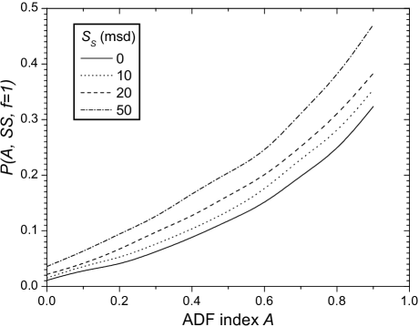
Figure 1.: The cumulative distribution of $P(A*)$ (see item iii) of Section S:as) for the reference data set for different values of the threshold observed area [$S_{\rm S}$] as denoted in the legend and the data coverage fraction $f$=1.Fig:cal

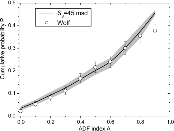
Figure 2.: The cumulative probability distribution function [$P(A)$] for observational data of R. Wolf (circles with error bars) together with the calibration curve (cf. Figure Fig:cal) for $S_{\rm S}=45$ msd and $f=0.66$ along with the uncertainties indicated by the shaded area. Fig:wolf

Thus, a set of calibration curves [$P(A,S_{\rm S},f)$] was constructed which is used to evaluate the quality of individual observer’s sunspot group detection as quantified in terms of “missing” spots with the area below the threshold $S_{\rm S}$.

2.2.2 Assessing the Observational Quality of Individual Observers

Sec:as In order to assess the quality of individual observers, we compared the functions [$P$] constructed for the data from that observer with the calibration curves as follows.

For a given observer with the daily observational coverage fraction [$f$], we defined, similarly to step ii) in Section S:cal, the monthly ADF index [$A$] and its distribution [$P(A,f)$]. Uncertainties of the $P$-values are considered statistical, similar to those in step iii) of Section S:cal. Then, for the given value of $f$ we fit the observer’s distribution to the calibration curves [$P(A,S_{\rm S},f)$] described above to find the value of $S_{\rm S}$, corresponding to the observer, and its uncertainty. The fit is done using the $\chi^{2}$ method for $P(A,S_{\rm S},f)$ in the range of $A$ between 0.1 and 0.8 (eight degrees of freedom). Small values of $A<0.1$ and higher values $A>0.8$ were not used because of low statistics and required high daily coverage within a month. Moreover, definition of very small and very large values requires a large number of observational days per month, which may distort the corresponding statistics for observers with poor coverage. The best-fit value of $S_{\rm S}$ is defined by minimizing the $\chi^{2}$-values, while uncertainties are defined as the range of $S_{\rm S}$ where the value of $\chi^{2}(S_{\rm S})$ lies below $\chi^{2}_{0}+1$ ($\chi^{2}_{0}$ being the minimum value) corresponding to the 68.3 % confidence interval.

An example of the fit is shown in Figure Fig:wolf for observations by R. Wolf (see Table Tab:Res). The $P$-distribution (dots with error bars) constructed for the data by Wolf is compared with the calibration curve for $S_{\rm S}=45$ msd and $f=0.66$ (the value of $f$ that applies to Wolf’s data). The dependence of the $\chi^{2}$-value on the value of $S_{\rm S}$ for Wolf’s data is shown in Figure Fig:chi2. For this particular observer the best-fit value of $S_{\rm S}$ is found to be 45 msd with the 68 % confidence interval being 36 to 53 msd. This means that, on average, Wolf did not see or report sunspot groups with an (observed) area smaller than 45 msd.

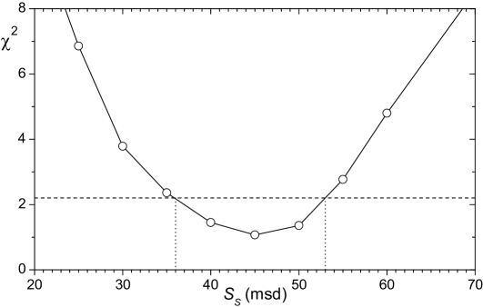
Figure 3.: Dependence of the $\chi^{2}$ of the fitting of Wolf’s data distribution to the calibration curves [$P(A,S_{\rm S},f=0.66)$] on the threshold value of $S_{\rm S}$. The horizontal dashed and vertical dotted lines illustrate the definition of the uncertainties.Fig:chi2

We also check for a potential source of error in that, since this method compares the ADF statistics of the real observations to those of the reference data set, it may depend on the level of solar activity during observations. If the observations were made during a period of very high activity, essentially higher than that averaged over the reference period, this method may yield the observer’s $P$-curves to that appear lower because of the smaller ADF. This may lead to a potential overestimate of the observer’s “quality” (underestimate of their personal observational threshold $S_{\rm S}$) and thus to an underestimate of the solar activity based on his/her observational data. Conversely, for low activity, the observer’s curve may appear higher, leading to an underestimate of his/her quality (overestimate of $S_{\rm S}$) and subsequently to an overestimate of solar activity. Since the calibration curves cover a period of moderate to high levels of activity (1900 – 1976), including the highest Cycle 19, the method overall tends to give a conservative lower limit of the observer’s quality (upper limit of the observational thresholds [$S_{\rm S}$]).

In order to check the dependence of the $S_{\rm S}$ on the activity level, we have composed synthetic pseudo-observers as subsets of the RGO data for the periods of low activity 1902 – 1923 (called RGO_low) and high activity 1944 – 1964 (RGO_high). By construction, these pseudo-observers have the true value of $S_{\rm S}=0$ since they are subsets of the reference RGO data set. Next we calibrated these pseudo-observers using the ADF method. We found that the formal threshold for the RGO_low observer is $S_{\rm S}$=$27\pm 10$ msd, i.e. the observer making observations during periods of low activity is likely to be over-calibrated (the threshold appears too high and, as a result, their observations, normalized to the reference data set, are overestimated). For the RGO_high pseudo-observer we found the value of $S_{\rm S}=-16\pm 5$ msd. The negative $S_{\rm S}$ means that we had to apply the observational threshold of 16 msd to the RGO_high data set in order to reproduce the ADF statistics for the reference data set with $S_{\rm S}$=0. This would potentially lead to a slight underestimate of the corrected data for such an observer. However, we note that the RGO_high pseudo-observer is an extreme case since the period around Cycle 19 was characterized by the highest activity in the entire sunspot-number series in all the existing sunspot series including SS15. We did not obtained a “negative” threshold for any real observer considered here. This implies that the method tends to provide an upper estimate of solar activity lying on the high side, particularly during periods of low-to-moderate activity. However, the test for RGO_low shows that during the grand minima the method cannot be applied. Future work will aim to establish calibrations for observers working during the Maunder minimum that are consistent with those derived here so that the data series can be extended back into the 17th century and the Maunder minimum.

We have identified 18 observers whose records can be calibrated by this method and form the core of the sunspot group historical series since the mid-18th century. They are listed in Table Tab:Res, along with the full ranges of observational dates, the periods used for calibration, the spotless day fraction and the obtained observational threshold [$S_{\rm S}$] with its $1\sigma$ uncertainties.

For the period of the late 19th and the 20th centuries we considered only a few key observers with long stable records since the quality and density of data during the last hundred years were high, and thorough studies of their inter-calibration have been performed (Clette et al., 2014). For the observers Quimby and Wolfer who have a significant overlap with the reference data set, we used the overlap period for a direct calibration.

For the period before the mid-19th century, all of the observers were considered and calibrated whenever possible following the method described here (i.e. whenever they had sufficient observations to apply our technique). For each observer we used data of sunspot group counts from the HS98 database (Hoyt and Schatten, 1998) except for Schwabe and Staudacher (see comments below). Whenever possible we used data for complete solar cycles. Unless indicated otherwise, we considered for each observer only months with three or more daily observations.

We also show in Table Tab:Res the spotless day fraction (SDF) which is the number of days with the reported absence of spots to the total number of observational days during the calibration period $T_{\rm cal}$, for each observer. The reference RGO data set contains $\approx 16$ % of spotless days. SDF is in the range of 15 % to 26 % for most of the observers in the 19th century except of Stark and Derfflinger whose observations were likely reflecting the low activity around the Dalton minimum. Apparently different from all other was Staudacher with only 57 spotless days (5.5 %) reported. He likely was more interested in drawing spots than reporting their absence. Whatever was the reason, his statistic of spotless/active days is distorted and cannot be used to calibrate his quality directly to the reference period, as discussed in Sect. Sec:Staud.

Some specific comments are given below.

S.H. Schwabe observed the Sun during 1825 – 1867; however we considered for calibration only the period of 1832 – 1867, covering three full cycles, since the earlier part of his record is thought to be of less stable quality (Leussu et al., 2013). Sunspot group numbers for Schwabe’s observations were taken not from the HS98 database but from a new revised collection by Arlt et al. (2013) (available at www.aip.de/Members/rarlt/sunspots/schwabe as version 1.3 from 12 August 2015).

For J.W. Pastorff from Drossen we used data for the observer # 263 in the HS98 database. His SDF is low (14 % – see Table Tab:Res) indicating that he might skipped reporting some spotless days. If this is true, it may lead to an overestimate of his observational quality and consequently to an underestimate of the sunspot group number based on his record. On the other hand, his corrected data is consistent with those of Schwabe and Stark (Figure Fig:all_m).

C. Horrebow from Copenhagen (observer #180 in the HS98 database) observed the Sun during 1761 – 1776. Here we use, for calibration, the period of 1766 – 1776 (one solar cycle) because the data are very sparse before 1766.

T. Derfflinger from Kremsmünster observed the Sun during 1802 – 1824, but we used for calibration data covering 1816 – 1824 to exclude the Dalton minimum so as to avoid the potential problems discussed above associated with a mismatch in the range of the data compared to that for the reference data set.

J.M. Stark from Augsburg observed the Sun during 1813 – 1836, and we use all data for the observer #255 of the HS98 database, while not considering the generic no-sunspot day records (observer #254 called “STARK, AUGSBURG, ZERO DAYS” in the HS98 database).

J.C. Schubert from Danzig observed the Sun during 1754 – 1758. We used for calibration the period of 1754 – 1757 which is $\pm 2$ years around the formal cycle minimum in 1755.2. This includes 404 daily observations with 36 % coverage. To assess the quality of Schubert’s observations we used the RGO statistics, as described in Section S:cal, but using RGO data only within $\pm$two years around the solar cycle minima to be consistent with Schubert’s cycle coverage.

J.C. Staudacher from Nürnberg, while providing about 1035 daily drawings for the period 1749 – 1795 ($\approx$6 % coverage), as published by Arlt (2008), cannot be directly calibrated in the way proposed here because he did not properly report days without sunspots. He reported no spots for only 5.5 % days which is less than all other observers (15 – 40 %, see Table Tab:Res). Moreover, there is no zero-spot months (with the number of daily observations more than two) in his record, in contrast to all other observers. This distorts the ADF statistics, making impossible direct calibration as described above. The case of Staudacher is considered separately in Section Sec:Staud.

The following observers produced sufficiently long observational records but cannot be calibrated in the manner described above because of sparse or unevenly distributed observations or because they did not report spotless days: Lindener, Tevel, Arago, Heinrich, Flaugergues, Hussey. We also did not consider observers during and around the Maunder minimum because of the very low level of activity (Usoskin et al., 2015) when the method cannot be applied. The period between the end of the Maunder minimum and the mid-18th century cannot be studied because of a lack of sufficient observations (Vaquero and Vázquez, 2009).

Table 1.: Results of calibration of the key observers used here. Columns are: Name of the observer; Period of observation $T_{\rm obs}$; Period used for calibration $T_{\rm cal}$; Number of observational days $N$ used for calibration; Data coverage in  % $f$; The fraction of spotless days (SDF) in the record; The threshold area $S_{\rm S}$ in uncorrected msd; values in parentheses denote the upper and lower 1$\sigma$ bound. For details see text.

Observer	$T_{\rm obs}$	$T_{\rm cal}$	$N$	$f$	SDF	$S_{\rm S}$
RGO	1874 – 1976	1900 – 1976	28644	$\approx 100\,\%$	16 %	0
Quimby	1889 – 1921	1900 – 1921c	10830	92 %	23 %	22$\left({}^{28}_{16}\right)$
Wolfer	1876 – 1928	1900 – 1928c	7165	68 %	21 %	6$\left({}^{12}_{\,0}\right)$
Winklera	1882 – 1910	1889 – 1910d	4812	60 %	24 %	53$\left({}^{66}_{45}\right)$
Tacchini	1871 – 1900	1879 – 1900d	6235	78 %	19 %	10$\left({}^{14}_{\,7}\right)$
Leppig	1867 – 1881	1867 – 1880d	2463	52 %	26 %	45$\left({}^{33}_{55}\right)$
Spoerer	1861 – 1893	1865 – 1893d	5386	53 %	15 %	3$\left({}^{5}_{0}\right)$
Weber	1859 – 1883	1859 – 1883	6981	79 %	19 %	22$\left({}^{28}_{16}\right)$
Wolf	1848 – 1893	1860 – 1893d	8102	66 %	21 %	45$\left({}^{53}_{36}\right)$
Shea	1847 – 1866	1847 – 1866	5538	79 %	20 %	25$\left({}^{33}_{18}\right)$
Schmidt	1841 – 1883	1841 – 1883	6887	49 %	21 %	10$\left({}^{15}_{\,\,6}\right)$
Schwabe	1825 – 1867	1832 – 1867	8570	65 %	18 %	13$\left({}^{18}_{\,\,8}\right)$
Pastorff	1819 – 1833	1824 – 1833d	1451	41 %	14 %	5$\left({}^{10}_{0}\right)$
Starka	1813 – 1836	1813 – 1836e	2406	30 %	41 %	60$\left({}^{70}_{50}\right)$
Derfflingera	1802 – 1824	1816 – 1824e	346	11 %	38 %	50$\left({}^{80}_{40}\right)$
Herschela	1794 – 1818	1795 – 1815	344	4 %	16 %	23$\left({}^{35}_{10}\right)$
Horrebow	1761 – 1776	1766 – 1776e	1365	34 %	27 %	75$\left({}^{95}_{60}\right)$
Schubert	1754 – 1758	1754 – 1757e	404	36 %	37 %	10$\left({}^{16}_{\,5}\right)$
Staudacherb	1749 – 1799	1761 – 1776	1035	14 %	5.5 %	–

Tab:Res
Notes: ^a – the observational threshold [$S_{\rm S}$] is likely overestimated.
^b – calibration is done via Horrebow (see Section Sec:Staud).
^c – direct overlap with RGO data set.
^d – to use complete cycles.
^e – see comments in Section Sec:as.

In addition we also checked the record by H. Koyama from Tokyo who observed the Sun over the period 1947 – 1984 with about 56 % daily coverage, data which formed one “backbone” for the method by SS15. We used for calibration the period of 1953 – 1976 to cover full cycles and to be more consistent with the RGO time interval, A total of 4778 daily observations were processed. The calibration was performed using the reference RGO dataset for the same period of time. The threshold [$S_{\rm S}$] value was found to be $8\pm 5$ msd, yielding a result fully consistent with the RGO data (see Figure Fig:all_m). We stress that this record was not used in the compilation of the final series, but only to test the method.

The calibration method works after 1754 when Schubert started observing. If Staudacher’s data is included (see Section Sec:Staud), the calibration starts in 1749. Before Staudacher there is a paucity of sufficiently long timeseries of observations by single observers, so that the method cannot work due to too poor statistics, and before 1715 the method is not applicable because of the Maunder minimum where the statistics of the reference data set cannot be applied. We stopped the calibration in 1900 since the reference data set of RGO data is used after 1900.

2.3 Corrections of Individual Observers

Sec:corr Once the observational threshold 8$S_{\rm S}$] and its uncertainty are defined for each observer (see above), observations (the number of sunspot groups) by this observer can be calibrated to the reference data set. All corrections are done at the daily scale, because of the non-linearity of correction that may otherwise distort the relation, as discussed below.

The correction, for a given range of $S_{\rm S}$-values (see Table Tab:Res), is made by the Monte-Carlo method using the reference data set of daily RGO group numbers in the following steps:

1. [i)]

2. A test value $S_{\rm S}^{*}$ is randomly selected, using the normally distributed random numbers, from the distribution of $S_{\rm S}$ values for the observer (see Table Tab:Res). A “degraded” subset of the reference daily data set is constructed by considering only sunspot groups with the (uncorrected) area $\geq S_{\rm S}^{*}$, i.e. what an observer with the observational limit of $S_{\rm S}^{*}$ would have recorded. For each daily value $G_{S_{\rm S}^{*}}$ from the degraded data set we construct a distribution of the $G_{\rm ref}$ values from the reference data set ($S_{\rm S}$=0), similar to that shown in Figure Fig:pdfb.

3. Step 1 above is repeated 1000 times, each time randomly selecting an $S_{\rm S}^{*}$ value for a given observer, and summing up all of the distributions of $G_{\rm ref}$ for a given $G_{S_{\rm S}^{*}}$ The probability density function (pdf) of the $G_{\rm ref}$ values for each $G_{S_{\rm S}^{*}}$ value (i.e. reported by the observer) is constructed. Finally, the correction matrix for the particular observer is constructed as illustrated in Figure Fig:pdfa.

4. For each daily recorded value [$G$] of the observer, the corresponding mean and the 68 % upper and lower quantiles of the $G_{\rm ref}$ were calculated, giving the mean corrected daily group number and its uncertainties.

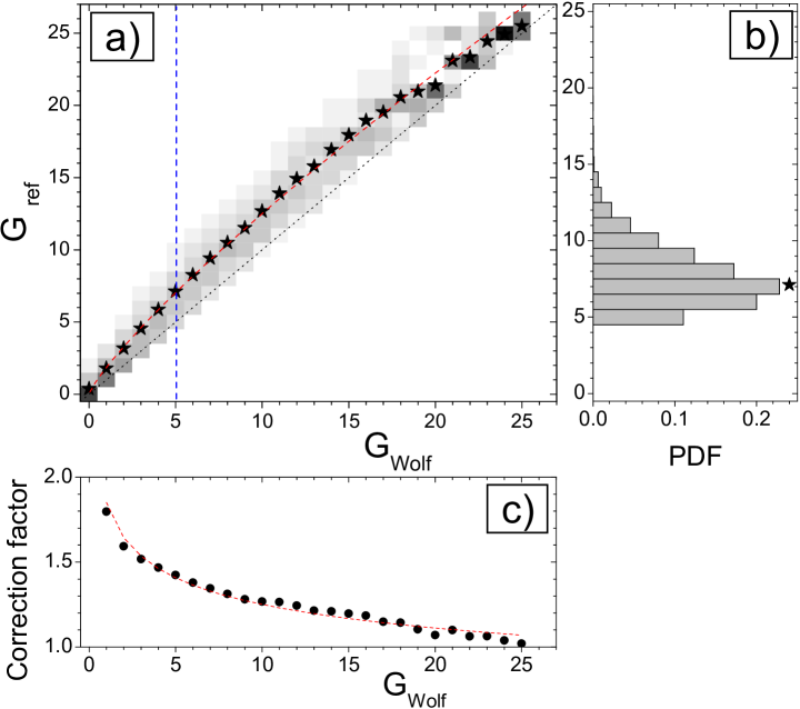
Figure 4.: a: Correction matrix for the data by R. Wolf: Distribution of the daily number of groups in the reference data set $G_{\rm ref}$ (ordinate) as a function of the number of groups $G_{\rm Wolf}$ reported by R. Wolf (abscissa). Each vertical strip is a probability density function (pdf). The grey scale is linear from 0 (white) to 1 (black) Stars represent the mean value of $G_{\rm ref}$ for the given $G_{\rm Wolf}$. The dotted line is the diagonal ($G_{\rm Wolf}=G_{\rm ref}$), and the dashed-red curve is the best-fit power law ($G_{\rm Wolfer}=1.85\cdot G_{\rm Wolf}^{0.83}$). Panel b: a cross-section of panel a at $G_{\rm Wolf}=5$ (vertical blue dashed line), the star denotes the mean value of the pdf (in this case at 7.12, making the optimum correction factor 7.12/5 = 1.424). The median at this example $G_{\rm Wolf}=5$ is $G_{\rm ref}=7.65$. Panel c: The optimum correction factor, viz. the ratio of the mean $G_{\rm ref}$ to $G_{\rm Wolf}$. The red-dashed line corresponds to the best-fit power law (see panel a). Fig:pdf

The method is illustrated in Figure Fig:pdf by calibration of the observational quality of R. Wolf from Zurich. The correction of an “imperfect” observer (R. Wolf in this example) is based on an assessment of how many sunspot groups the “perfect” observer (the reference RGO in our case) would see for a day when the “imperfect” observer reported $G_{\rm Wolf}$ groups. Thus, for a given $G_{\rm Wolf}$ value ($x$-axis) one obtains a pdf of the reference values [$G_{\rm ref}$] to yield the mean and the uncertainties of the corrected number of sunspot groups. We note that the relation is well-approximated by a power law with the spectral index 0.83 (the dashed red curve in Figure Fig:pdf), but this functional form is shown only for illustration and not used in the construction of correction matrices. An important feature observed is that the mean $G_{\rm ref}$ value is non-zero (0.38) for spotless days reported by an “imperfect” observer, R.Wolf in our example. Accordingly, we cannot say whether zero spots by Wolf implies a true spotless day or whether groups were small and went undetected. It is important that the correction implied by the matrix cannot be approximated by a linear (or worse still, a proportional) regression. Panel c of Figure Fig:pdf depicts the daily correction factor defined as the ratio of the $G_{\rm ref}$ (the number of groups the real observer would see if they would be a perfect observer) to $G_{\rm Wolf}$ (the number of groups the observer R. Wolf actually reported). The ratio gradually drops from $\approx 1.8$ for one group reported by Wolf to 1.19 for 15 groups reported by Wolf. If Wolf saw 25 groups, the correction would have been only 1.02. This implies that the larger the number of sunspot groups is (the higher the activity is), the smaller is the relative error of the “imperfect” observer. It is clear that a simple linear regression cannot be used to correct an “imperfect” observer (see Section Sec:nonlin). This was also emphasized by Lockwood et al. (2015) from a study of the effects of imposing different observational thresholds on the RGO data.

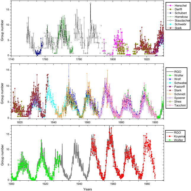
Figure 5.: Monthly series of sunspot group numbers obtained by individual observers, after corrections for the observational “imperfectness” (uncertainties are nor shown).Fig:all˙m

From daily values for each observer, corrected for the “imperfectness” as described above, we have calculated monthly $G_{\rm ref}$ values for individual observers, as a weighted (with weight being inversely proportional to the squared error of the daily corrected value) average of the available daily values. We stress again that the correction should be applied to the daily values, not to monthly, or even worse, annual averages, because of the nonlinearity of the correction (see Section Sec:nonlin). Such series of the monthly $G_{\rm ref}$, scaled to the reference data set of RGO, are shown in Figure Fig:all_m for some individual observers. One can see that the different observers, after correction, agree well with one another, even though the corrections were done totally independently for each observer.

2.3.1 Calibration of Staudacher via Horrebow

Sec:Staud

J.C. Staudacher is a key observer to evaluate solar activity in the second half of the 18th century and a “backbone” observer for SS15. It is crucially important to evaluate the quality of the data he produced. However, since he apparently did not properly (see Table Tab:Res) report spotless days, being primarily interested in drawing sunspots, the ADF method used here cannot be directly applied to his data, and it would yield an unrealistically high quality of observations. Accordingly, we have made a two-step calibration of Staudacher data to the reference data set. This is the only exception to the method described above.

First we directly calibrated Staudacher’s data to those recorded by C. Horrebow from Copenhagen (observer # 180 of the HS98 database), whose quality is evaluated by the ADF method (Table Tab:Res). We used the period of direct overlap of the two observers in 1761 – 1776. Staudacher’s data were digitized recently by Arlt (2008) who processed his original drawings. The sunspot groups were redefined (R. Arlt, personal communication 2015) using these drawings (Senthamizh Pavai et al., 2016). We note that this dataset is different from the HS98 database, in particular in that it yields $\approx 30$ % more sunspot groups. Horrebow’s data were taken from the HS98 database as being robustly defined (R. Arlt, personal communication, 2015). We found 110 days when both observers reported observations. In order to improve statistics we compared also the neighboring $\pm$two days. This added 101 cases when the observations were in successive days, and 39 days when they were separated by two days. We note that, as discussed by Willis, Wild, and Warburton (2015) in their survey of the early RGO data, there are some sunspot groups that last for only one day, but they are infrequent and likely near or below the $S_{\rm S}$ threshold for Staudacher and Horrebow, anyway. Accordingly, the possible error introduced by using neighboring days is greatly outweighed by the reduction in uncertainty brought about by having a greater number of samples, more than doubling the statistics. First we checked, for each daily observation by Staudacher, if there was a coincident record from Horrebow and took this pair if it existed in the positive case. If such a counterpart was not found, we looked for an adjacent ($\pm$one day) observation by Horrebow and took that pair if it existed. Otherwise, we considered the $\pm$two days interval. This gives in total 250 pairs of “coincident” data days by Staudacher and Horrebow. A cross-matrix of such daily values Staudacher vs Horrebow was constructed as shown in Figure Fig:Staud.

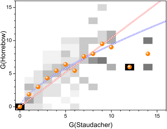
Figure 6.: The pdf matrix of conversion of daily group numbers between Staudacher and Horrebow ($G_{\rm Staud}$ and $G_{\rm Horr}$, respectively) using direct data for overlapping (within $\pm$two days) days. The grey scale is linear from 0 (white) to 1 (black). Orange balls are the mean values. For illustration the best-fit linear proportionality ($G_{\rm Horr}=1.04\cdot G_{\rm Staud}$ red line) and power-law ($G_{\rm Horr}=1.91\cdot G_{\rm Staud}^{0.69}$) are shown. The two last points were not used in the analysis. Fig:Staud

One can see that the two observers are close to each other in the quality of observations (the matrix is nearly diagonal) except for the two right-most points, where Staudacher drew significantly more groups than reported by Horrebow. A matrix for converting Staudacher’s daily values of $G$ into Horrebow’s values is constructed in a similar way to those above for all other observers with respect to the reference data set.

Next, we applied the correction matrix of Horrebow-to-reference data set and finally converted Staudacher’s daily number of groups into the reference data set as follows:

$$G_{\rm Staud}\stackrel{{\scriptstyle R_{1}}}{{\longrightarrow}}G^{{}^{\prime}}_{\rm Horr}\stackrel{{\scriptstyle R_{2}}}{{\longrightarrow}}G_{\rm ref}\ilabel{Eq:a}$$

For each daily value $G_{\rm Staud}$ we randomly selected (step $R_{1}$) the value of $G^{{}^{\prime}}_{\rm Horr}$ from the matrix described above (i.e. randomly from all values corresponding to $G_{\rm Staud}$), and then, for this $G^{{}^{\prime}}_{\rm Horr}$ we randomly selected a value of $G_{\rm ref}$ from the Horrebow correction matrix (from within the row corresponding to $G^{{}^{\prime}}_{\rm Horr}$). This procedure was repeated 1000 times, and finally the correction matrix of Staudacher [$G_{\rm Staud}$] daily values to the reference data set [$G_{\rm ref}$] was constructed.

2.3.2 Test of the Correction: Wolf-vs-Wolfer

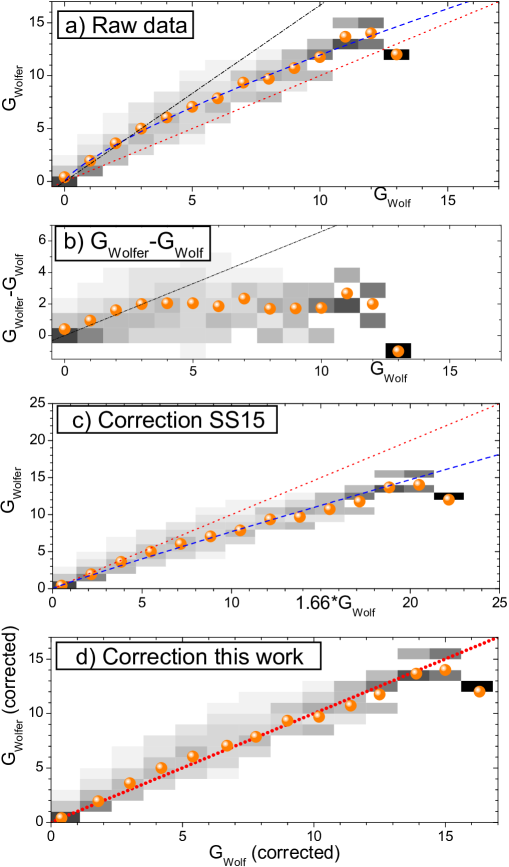
Figure 7.: Comparison of daily group numbers by Wolfer and Wolf for days when both have records (4385 days of simultaneous records), presented as a pdf (grey scale from 0 (white) to 1 (black)). The orange balls represent the mean values of $G_{\rm Wolfer}$ in each bin of $G_{\rm Wolf}$ values. The red line depicts the diagonal ($G_{\rm Wolf}=G_{\rm Wolf}$). Panel a presents raw (uncorrected) daily group numbers in the HS98 database. The blue dashed line is the best-fit power law ($G_{\rm Wolfer}=2.03\cdot G_{\rm Wolf}^{0.77}$), the black dash-dotted line is the relation $G_{\rm Wolfer}=1.66\times G_{\rm Wolf}$ (used by Clette et al. (2014) and SS15). Panel b depicts the distribution of the difference between $G_{\rm Wolfer}$ and $G_{\rm Wolf}$ daily group numbers as a function of $G_{\rm Wolf}$. Panel c presents data by Wolf multiplied by 1.66 as proposed by SS15. Blue dashed curve is the best-fit power law ($G_{\rm Wolfer}=0.89\cdot G_{\rm Wolf}^{0.94}$), Panel d presents data of both observers corrected to the reference conditions as proposed in this work. Fig:wolf˙wolfer

A good and important example to test our and other calibration methods is the relation between data reported by J.R. (Rudolf) Wolf and H.A. (Alfred) Wolfer, both from the Zurich observatory. First, a proper comparison of the two observers is crucially important as Wolf was the reference observer for the Wolf sunspot number series, while Wolfer is the reference observer for the ISN (v.2) and a “backbone” observer for the SS15 reconstruction. Without an adequate comparison between them, it is difficult to compare the various sunspot series now available. Second, a long period of their overlap (4385 days during 1876 – 1993) exists when both observers independently reported sunspots. HS98, using a linear regression applied to the daily values of the overlapping periods, proposed that the two observers are quite close to each other in the quality of their observations. In contrast, SS15 proposed, using a linear-regression analysis of the annually averaged number of sunspot groups, that the relation between them is a linear and proportional scaling so that $G_{\rm Wolfer}=1.66\times G_{\rm Wolf}$.

Figure Fig:wolf_wolfera shows the scatter plot (in the form of a pdf as in Figure Fig:pdfa) of the 4385 simultaneous daily values of $G_{\rm Wolfer}$ and $G_{\rm Wolf}$. One can see that Wolfer reported systematically more groups than Wolf, but the relation is significantly nonlinear. In fact, as illustrated in Figure Fig:wolf_wolferb, Wolfer systematically reported a few groups more than Wolf, at all levels of solar activity (see Section Sec:nonlin). It is evident that such a nonlinear relation cannot be approximated by a single linear scaling of 1.66. The black dash–dotted line represents the linear scaling 1.66 as proposed by SS15 and, although it reasonably describes low-activity periods ($G_{\rm Wolf}<4$), it progressively overestimates the number of groups by Wolf for high activity. For example, for a day with 10 groups reported by Wolf, this scaling would imply 16 – 17 groups reported by Wolfer. But Wolfer never reported more than 13 groups for days with $G_{\rm Wolf}=10$ (the mean for such days was $G_{\rm Wolfer}=11.75$). It is therefore clear that the results obtained by applying the linear scaling ($G_{\rm Wolfer}=1.66\times G_{\rm Wolf}$) contradict the data. This is also seen in Figure Fig:wolf_wolferc, which shows the scatter of the Waldmeier raw daily data and the scaled (with a factor 1.66 as proposed by SS15) data of Wolf. One can see that the scaling by SS15 introduces very large errors at high levels of solar activity, making a moderate level appearing as high. This is a primary reason of high solar cycles claimed by SS15 and Clette et al. (2014) in the 18th and 19th centuries.

Figure Fig:wolf_wolferd shows the relation of the simultaneous-day group numbers by the two observers, after the correction performed here (reduction to the reference RGO data set). One can see that the data are nearly perfectly corrected – the corrected data lie around the diagonal implying that both series report the same quantity. The best-fit to the orange balls (the last point excluded) is $G^{*}_{\rm Wolfer}=(0.98\pm 0.03)\times G^{*}_{\rm Wolf}$, where the asterisks denote the values calibrated to the reference data set. We remind the reader that Wolf and Wolfer were calibrated to the reference data set independently of each other, and thus this comparison provides a direct test of the validity of the method. The ratio $G^{*}_{\rm Wolfer}/G^{*}_{\rm Wolf}$ should, of course, be unity if the calibration is done correctly: that this is the derived value within the uncertainty shows that both have been properly estimated. Thus, since the ratio between the daily group numbers (for the days when both observers made observations) of Wolf and Wolfer is consistent with unity (i.e. one-to-one relation) after each of them was independently corrected, we conclude that the method works well. We note that this example is shown only for illustration and not used in the actual calibration.

3 Corrected Series of Sunspot Group Numbers

In this section we construct a composite series of sunspot group numbers for the period since 1749 using the selected observers.

3.1 Compilation of the Corrected Series

S:compil For each day [$t$] we considered all those observers whose reports are available for that day. For each such observer $i$ we took the reported $G_{{\rm obs},i}$ value for that day and corrected it to the reference data set using the correction matrix for that observer (as described in Section Sec:corr) to define the pdf of the corresponding values [$G_{{\rm ref}}$]. If several observers are available for the day, the corresponding pdfs were multiplied and re-normalized to unity again. In order to avoid possible voiding of the observational days with an outlying data, we set the minimum pdf values to $10^{-4}$. Then, from such composite (over all of the observers for the day) pdfs we calculated the mean daily value of $G_{\rm ref}$ and its 68 % error as the standard deviation from the gathered pdf divided by $\sqrt{N}$ where $N$ is the number of observers for the day.

From these composite daily series we constructed a monthly composite series as a standard weighted average (see details given in, e.g. Usoskin, Mursula, and Kovaltsov, 2003) of the composite daily values. This series is available in the electronic supplement to the article.

The work by Usoskin, Mursula, and Kovaltsov (2003) shows that it is not optimal to calculate the annual value of the composite series as an (arithmetic or weighted) average of the monthly values. For example, if the year in question is in the rising phase of an activity cycle, the value of $G$ may increase significantly between January and December, rising by up to an order of magnitude. For example, in 1867 the monthly $G$ was 0.15 in January and 1.6 in December. If accidentally, the month of December had better coverage and a smaller error of the monthly value than January, the annual weighted mean would be dominated by the December value, which is obviously incorrect. Therefore we use a Monte-Carlo procedure to calculate the annual $G$ value and its uncertainties from the daily $G$-values with errors:

1. [i)]

2. For each day with existing data within the given year, we took randomly a value of daily $G$ from the composite pdfs of corrected daily $G$-values obtained above.

3. From these randomly taken daily $G$-values we computed the monthly values as the simple arithmetic mean.

4. The annual value $G^{{}^{\prime}}$ was computed as the arithmetic mean of the monthly values.

5. Steps i) – iii) were repeated 1000 times so that a distribution of the annual $G^{{}^{\prime}}$ values was obtained. Finally, the mean and the 68 % (divided by the $\sqrt{n}$, where $n$ is the number of the months with data in the year) were computed from the distribution. Errors propagate naturally and without biases in this approach.

This annual series with 68 % uncertainties is shown in Figure Fig:all_y. It covers the period 1749 – 1899, with one missing value in 1811. To complete the series and bring it up to the present day, we use group numbers from the RGO data set for the period 1900 – 1976. After that we used complete series by sunspot group numbers from the Solar Optical Observing Network (SOON), funded by the United States Air Force and NOAA with filling of some data gaps using the “Solnechniye Danniye (Solar Data, SD) Bulletins issued by the Main Astronomical Observatory of Russian Academy of Science (Pulkovo, St. Petersburg, Russia). The main SOON observations are from Boulder with support stations at Holloman, Learmonth, Palehua, Ramey, San Vito, and Mount Wilson. Unlike the RGO data, the SOON data are recorded as drawings rather than photographic plates. We use the RGO-SOON group number intercalibration derived by Lockwood, Owens, and Barnard (2014), which employs the international sunspot number as a spline and minimizes the difference between the means of the fit residuals for before and after the RGO/SOON join.

One can see that the activity remains at a moderate level in the 19th century, and is higher in the 18th century. However, activity (sunspot group numbers) in both the 18th and 19th centuries remained significantly lower than the Modern Grand Maximum in the second half of the 20th century.

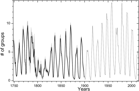
Figure 8.: Annual number of sunspot groups for the period 1749 – 1900 (solid curve) normalized to the reference data set, along with 68 % confidence interval (grey shading). The reference data set of RGO group numbers for 1900-1976, extended by the SOON data 1977 – 2013, as normalized to the RGO set by Lockwood et al. (2014), is represented by the dotted curve. Fig:all˙y

We also note that there is another source of non-linearity not accounted for here (neither was it considered in previous series, such as HS98, ISN or SS15). It is related to calculation of monthly and annual values from a small number of sparse daily observations. Under such conditions, the simple arithmetic average tends to overestimate the number of sunspots (groups) for active periods, if the number of daily observations per month is smaller than three (Usoskin, Mursula, and Kovaltsov, 2003). The overestimate can be as much as 20 – 25 %. This may affect the values for the 18th century where data coverage was low. Since this effect leads to a possible overestimate of the monthly (and thus annual) values, it keeps the averaged series provided here as a conservative upper limit. However, this effect does not influence the calibration and correction procedure which works with the original daily data. Neither is the corrected daily series affected. This effect will be taken into account in forthcoming studies.

3.2 Comparison to Previous Reconstructions

Here we compare the new series with two earlier series of the number of sunspot groups: the GSN series by HS98 based on consecutive mutual calibration of observers; and the recent series by SS15 based on a composite of “backbone”, “high-low activity”, and “brightest star” methods. In Figure Fig:comp we show these series along with the recent reconstruction of sunspot activity around the Maunder minimum using active-day statistics (Vaquero et al., 2015).

One can see that the new series is close to the GSN series by HS98, being consistent with it within uncertainties after $\approx$1830 and yielding cycles #10 and 11 slightly higher than in the HS98 series. The newly reconstructed cycles are significantly higher than the HS98 values before 1830. On the other hand, the new series is consistently lower than the values proposed by SS15, except for the years of the sunspot cycle minima. This difference is mostly due to the linear regression used by SS15 to correct the Wolf-vs-Wolfer records which leads to a bias, as discussed in Section Sec:nonlin. Before 1830 the new series lies between the HS98 and SS15 series, on one hand being consistent with the conclusion by SS15 that the HS98 GSN is likely too low before the Dalton minimum, but on the other hand implying that the revision by SS15 is too high. We recall that because of the moderate to high activity underlying the reference data set, our reconstruction tends to overestimate reconstructed activity at earlier times with lower activity. Note that the RGO data and the SS15 series also diverge around 1945 and tests by Lockwood, Owens, and Barnard (2015) against independent data indicate that this is another error in the backbone reconstruction. The two errors (around 1945 and the Wolf-vs-Wolfer relationship) both act in the same direction, to make early group sunspot numbers too large in relation to those in the Modern Grand Maximum.

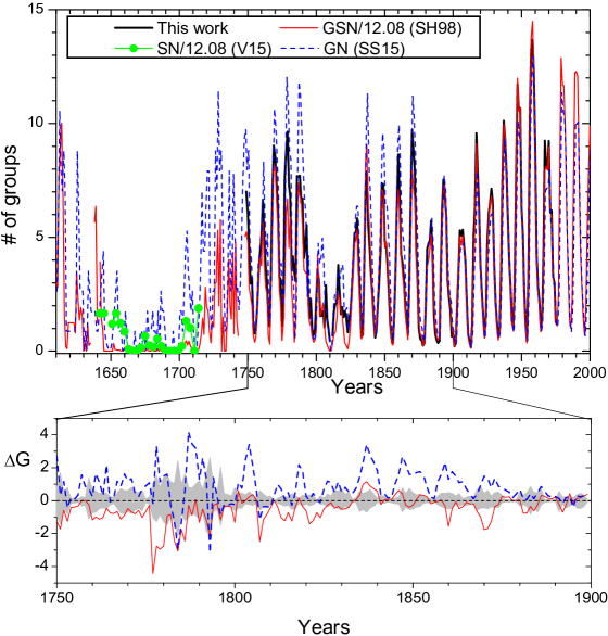
Figure 9.: Comparison of different series of annual numbers of sunspot groups $G$: solid black curve – the present reconstruction (identical to that shown in Figure Fig:all_y); red dotted curve – group sunspot number (HS98) divided by 12.08; blue dashed curve – number of groups reconstructed by ss15; green dotted curve – sunspot number divided by 12.08 around the Maunder minimum as reconstructed by the strict model of Vaquero et al. (2015). The lower panel is the difference between the two other $G$ series shown in the upper panel and the present result, for the period 1749-1899. Also plotted in the lower panel (shaded area) is the 68 % uncertainty estimate of the present data set. Fig:comp

The new reconstruction suggests that the sunspot activity (quantified as the number of groups) was somewhat higher in the mid-18th century than it was in the mid-19th century but significantly lower than the Modern Grand Maximum of activity (Usoskin et al., 2003; Solanki et al., 2004) in the second half of the 20th century. The Dalton (ca. 1800) and Gleissberg (ca. 1900) lows of solar activity are clearly seen as the reduced magnitude of solar cycles, but they are not considered as grand minima of activity in contrast to the Maunder minimum (Usoskin, 2013).

4 A Note on Non-linearity and the Lack of Proportionality

Sec:nonlin The main reason for the difference between the sunspot activity levels resulting from this work and previous recent reconstructions (e.g. Clette et al., 2014; Svalgaard and Schatten, 2015) is that the latter were based on linear regressions between annually averaged data of individual observers, which can seriously distort the results. Furthermore, SS15 assumed proportionality between the data (by forcing linear regressions through the origin and using only scaling correction factors without offsets) which is also incorrect and leads to possible errors which accumulate because the “backbone” calibrations are daisy-chained (Lockwood et al., 2015). For example the linear regression suggests a ratio of 1/0.6=1.66 between the numbers of sunspot groups reported by Wolf and Wolfer. This assumes that Wolf was missing 40 % of all groups that would have been observed by Wolfer irrespectively of the activity level, viz. a no-spot record by Wolf would correspond to no spots observed by Wolfer, but 15 groups reported by Wolf would correspond to 25 groups by Wolfer. As we show here, a linear regression (proportionality) based on the annually averaged data may lead to significant biases leading to a heavy overestimation of the number of sunspot groups recorded by Wolf during the periods of high activity.

The relation between records of different observers is non-linear (see, e.g., Figure Fig:pdfa for Wolf). First, it does not necessarily go through the origin (0-0 point). Thus $G_{\rm Wolf}=0$ yields a nonzero $G_{\rm ref}$ with a mean of 0.49 and the 68 % range from 0 to 2 groups. This indicates that, when Wolf reported no spots, there might have been 0 – 2 groups on the Sun. This feature is totally missed when assuming a linear proportionality. The relation between Wolf and Wolfer is quite steep (the slope of a regression forced through the origin is about 1.7) for low activity days (1 – 2 groups) but then the slope of the relation drops (see Figure Fig:pdfc) to almost unity for days with more than 20 groups. It is obvious that a single correction factor is not applicable for such a relation as it assumes that an “imperfect” observer (Wolf in this case) misses the same fraction of spots irrespectively of the activity level. However, the non-linearity of the relation is due to the fact that an observer with a poorer instrument or eyesight, or observing in poorer conditions, does not see and report the smallest spots as defined by their observational threshold $S_{\rm S}$.

It is important that the fraction of small spots is not constant as proposed by the linear correction, but depends strongly on the level of solar activity. It is usually large for a small number of groups and small for multiple groups, as illustrated in Figure Fig:frac for the case of Wolf.

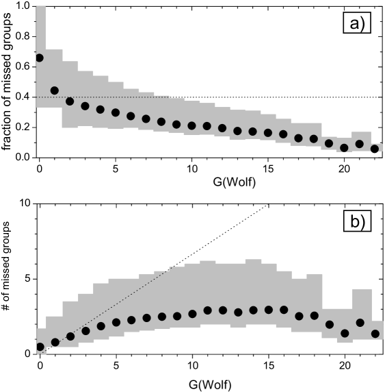
Figure 10.: Assessment of small-size groups potentially missable by R. Wolf using the statistics of the reference data set (daily RGO sunspot groups with their size for the period 1900 – 1976) as shown in Figure Fig:pdfa. Panel a: the fraction of the missable sunspot groups as a function of the number of sunspot groups visible for Wolf. Panel b: the absolute number of missable sunspot groups as a function of the number of sunspot groups visible for Wolf. The solid dots and the grey shading depict the mean and the 68 % confidence intervals, respectively. The dotted line indicates the constant 40 % fraction of missed spot groups as assumed by the linear regression. Fig:frac

While the fraction of small groups (panel a), potentially missed by Wolf, is as high as 45 % for the days when he would report only one sunspot group, it drops very quickly, so that it is only 21 % for days with 10 groups reported and 10 % for very active days with the number of reported groups being 16. One can see that the assumption of a constant fraction of missed groups (the dotted line) does not describe the distribution, and it heavily overestimates the missed group for moderate and high activity. From panel b one can see that, for moderate and high activity (daily $G>4$), Wolf would have been missing the same amount of 2 – 3 groups on average, irrespective of the exact number of groups he saw (cf. Figure Fig:wolf_wolferb). The assumption of the constant fraction of missed groups (the dotted line with the slope 0.6667=0.4/0.6) is apparently invalid and is applicable only for low-activity days ($G<4$). This suggests that not a multiplicative (via a scaling factor) but an additive (with an offset) correction would be more appropriate for moderate-high activity days. However, the most appropriate way to correct a given observer (Wolf in this example) is to apply the correction matrix (Figure Fig:pdf) to daily group numbers observed by them as described here.

Another problem with linear regressions is that, because of the non-linearity, the averaging procedure is not transmissive for corrections, i.e., the correction of the averaged values is different from the average of corrected values. Corrections must be applied to daily values using a matrix as shown in FigureFig:pdf, and only after that can the corrected values be averaged to monthly or yearly resolution, as described in Section Sec:corr. Corrections applied to (annually) averaged values miss the non-linearity and, since the annual values are dominated by low and moderate numbers of groups, lead to an overestimate of the relation and, as a consequence, to too high solar cycles. Moreover, the use of simple arithmetic means from sparse daily values may lead to an additional overestimate of the monthly (or annual) values thus distorting the relation (Usoskin, Mursula, and Kovaltsov, 2003, see discussion in Section S:compil). A weighted average should be used instead.

Accordingly, the use of annual (or even monthly) averaged values for a linear scaling correction is not appropriate and is grossly misleading.

A different average size of sunspot groups as a function of activity level producing such a non-linearity is known in solar physics (e.g., Solanki and Unruh, 2004). e.g., the ratio of faculae to spots changes with activity level (i.e. the ratio of number of small to large magnetic flux tubes). Of course neither faculae-to-spot area ratio nor sunspot areas directly enter into the number of sunspot groups or the size of groups, but they are examples of other (somewhat related) quantities showing a non-linear behaviour.

5 Conclusions

A new series of sunspot-group numbers, based on a novel method of independent calibration of the quality of data by different sunspot observers, is presented for the period 1749 – 1900. These data have been calibrated using as the reference data set the one from the Royal Greenwich Observatory for the period 1900 – 1976, which is readily extended to the present day using the SOON data, forming a homogeneous series for the entire period since 1749 – 1976 (see Figure Fig:all_y). The new series is a composite of 18 individual observers (Table Tab:Res), each being independently calibrated to the reference data set using the newly developed active-day fraction method. It is important that the new method provides independent direct calibration, using the active-day fraction statistics, of the observers to the reference data set in the sense of the observational threshold, thus avoiding consecutive error accumulation, in contrast to earlier methods. The method includes several main steps:

1. [i)]

2. constructing calibration curves for the reference data set;

3. assessing the quality of individual observers in terms of the observational threshold of the sunspot group area [$S_{\rm S}$];

4. normalizing raw data by the individual observers to the reference data set;

5. compiling the composite series.

The method does not use any linear regressions or other prescribed functional relations, but is, instead, based on a direct correction matrix and the Monte-Carlo method. The basic assumptions of the method are:

• The reference data set is of the “perfect” quality, and the ADF statistic for this set is representative for the entire period under investigation. The selection of the reference data set ensures that violations of this assumption may only lead to a possible overestimate of the activity.

• The quality of an observer is quantified as the observational threshold [$S_{\rm S}$], so that the observer misses all groups with an area smaller than $S_{\rm S}$ and reports all groups with an area greater than $S_{\rm S}$, and the quality remains constant throughout their entire period of observations, but this can be revisited in the future by a piece-wise calibration.

• The correction of an “imperfect” observer is based on an estimate of the number of groups (s)he would see if (s)he was a “perfect” observer (i.e., with the data quality corresponding to the reference data set).

The series presented here is a basic skeleton, or core, of the reconstruction of the number of sunspot groups, to which other observers with shorter sunspot records can and will be added later by means of direct normalization to this core series. The raw series includes daily numbers of sunspot groups, the mean values and their 68 % confidence intervals, reduced to the reference data set, for each individual observer listed in Table Tab:Res. The composite series exists, in addition to raw daily resolution, as monthly and annual averages provided in the Electronic Supplementary Material.

The new series is consistent with the Group Sunspot Number (Hoyt and Schatten, 1998) after about 1830 but is systematically higher than that in the 18th century, implying that the sunspot activity was higher than proposed by HS98 before the Dalton minimum. Conversely, the new series is significantly and systematically lower than the “backbone” sunspot group number SS15 in the 19th and 18th century, implying that the “backbone” reconstruction grossly overestimates solar activity during that period. We demonstrated that the overestimate of the “backbone” method was caused by the incorrect use of linear proportionality to normalize the observers to each other, which led to propagation and accumulation of errors. Furthermore, the use of annual means of sparse data led to additional errors, enhancing those for observers active at earlier times.

The new series depicts lows of solar activity around 1800, known as the Dalton minimum, and around 1900, known as the Gleissberg minimum, although they are not considered as grand minima of activity. We note that the new series provides an upper limit for the group numbers during most of the times, in particular around the Dalton minimum, when both the activity level and the observation density were low. The Modern Grand Maximum of activity in the 20th century is confirmed as a unique event over the last 250 years. This confirms and enhances the established pattern of the secular variability of solar activity (e.g. Hathaway, 2015; Usoskin, 2013).

Acknowledgements

We are thankful to Rainer Arlt for the revised data of Staudacher. Contributions from I. Usoskin, K. Musrsula and G. Kovaltsov were done in the framework of the ReSoLVE Centre of Excellence (Academy of Finland, project no. 272157). Work at the University of Reading is supported by the UK Science and Technology Facilities Council under consolidated grant number ST/M000885/1. G. Kovaltsov acknowledges partial support from Programme No. 7 of the Presidium RAS. This work was partly supported by the BK21 plus program through the National Research Foundation (NRF) funded by the Ministry of Education of Korea.

Disclosure of Potential Conflicts of Interest

The authors declare that they have no conflicts of interests.

References

- Arlt (2008) Arlt, R.: 2008, Digitization of sunspot drawings by staudacher in 1749 – 1796. Solar Phys. 247, 399. DOI. ADS.
- Arlt et al. (2013) Arlt, R., Leussu, R., Giese, N., Mursula, K., Usoskin, I.G.: 2013, Sunspot positions and sizes for 1825-1867 from the observations by Samuel Heinrich Schwabe. Mon. Not. Royal Astron. Soc. 433, 3165. DOI.
- Balmaceda et al. (2009) Balmaceda, L.A., Solanki, S.K., Krivova, N.A., Foster, S.: 2009, A homogeneous database of sunspot areas covering more than 130 years. J. Geophys. Res. 114, A07104. DOI. ADS.
- Baumann and Solanki (2005) Baumann, I., Solanki, S.K.: 2005, On the size distribution of sunspot groups in the Greenwich sunspot record 1874-1976. Astron. Astrophys. 443, 1061. DOI. ADS.
- Çakmak (2014) Çakmak, H.: 2014, A digital method to calculate the true areas of sunspot groups. Experim. Astron. 37, 539. DOI. ADS.
- Clette et al. (2014) Clette, F., Svalgaard, L., Vaquero, J.M., Cliver, E.W.: 2014, Revisiting the sunspot number: A 400-year perspective on the solar cycle. Space Sci. Rev. 186, 35. DOI.
- Cliver and Ling (2015) Cliver, E.W., Ling, A.G.: 2015, The Discontinuity in 1885 in the Group Sunspot Number. Solar Phys. (in press).
- Eddy (1976) Eddy, J.A.: 1976, The maunder minimum. Science 192, 1189. DOI. ADS.
- Harvey and White (1999) Harvey, K.L., White, O.R.: 1999, What is solar cycle minimum? J. Geophys. Res. 104, 19759. DOI. ADS.
- Hathaway (2015) Hathaway, D.H.: 2015, The solar cycle. Living Rev. Solar Phys. 12, 4. DOI. http://www.livingreviews.org/lrsp-2015-4.
- Hoyt, Schatten, and Nesmes-Ribes (1994) Hoyt, D.V., Schatten, K.H., Nesmes-Ribes, E.: 1994, The one hundredth year of rudolf wolf’s death: Do we have the correct reconstruction of solar activity? Geophys. Res. Lett. 21, 2067. DOI. ADS.
- Hoyt and Schatten (1992) Hoyt, D.V., Schatten, K.H.: 1992, New information on solar activity, 1779-1818, from Sir William Herschel’s unpublished notebooks. Astrophys. J. 384, 361. DOI. ADS.
- Hoyt and Schatten (1995a) Hoyt, D.V., Schatten, K.H.: 1995a, A new interpretation of Christian Horrebow’s sunspot observations from 1761 to 1777. Solar Phys. 160, 387. DOI. ADS.
- Hoyt and Schatten (1995b) Hoyt, D.V., Schatten, K.H.: 1995b, A revised listing of the number of sunspot groups made by Pastorff, 1819 to 1833. Solar Phys. 160, 393. DOI. ADS.
- Hoyt and Schatten (1996) Hoyt, D.V., Schatten, K.H.: 1996, How well was the sun observed during the maunder minimum? Solar Phys. 165, 181. DOI. ADS.
- Hoyt and Schatten (1998) Hoyt, D.V., Schatten, K.H.: 1998, Group sunspot numbers: A new solar activity reconstruction. Solar Phys. 179, 189. DOI. ADS.
- Kovaltsov, Usoskin, and Mursula (2004) Kovaltsov, G.A., Usoskin, I.G., Mursula, K.: 2004, An upper limit on sunspot activity during the Maunder minimum. Solar Phys. 224, 95. DOI. ADS.
- Leussu et al. (2013) Leussu, R., Usoskin, I.G., Arlt, R., Mursula, K.: 2013, Inconsistency of the Wolf sunspot number series around 1848. Astron. Astrophys. 559, A28. DOI.
- Lockwood, Owens, and Barnard (2015) Lockwood, M., Owens, M.J., Barnard, L.: 2015, Tests of sunspot number sequences: 4. The “Waldmeier discontinuity” in various sunspot number and sunspot group number reconstructions. Solar Phys., (in press).
- Lockwood, Owens, and Barnard (2014) Lockwood, M., Owens, M.J., Barnard, L.: 2014, Centennial variations in sunspot number, open solar flux, and streamer belt width: 1. Correction of the sunspot number record since 1874. J. Geophys. Res., Space Phys. 119, 5172. DOI. ADS.
- Lockwood et al. (2006) Lockwood, M., Rouillard, A.P., Finch, I., Stamper, R.: 2006, Comment on “The IDV index: Its derivation and use in inferring long-term variations of the interplanetary magnetic field strength” by Leif Svalgaard and Edward W. Cliver. J. Geophys. Res. 111, A09109. DOI. ADS.
- Lockwood et al. (2015) Lockwood, M., Owens, M.J., Barnard, L., Usoskin, I.G.: 2015, Tests of sunspot number sequences: 3. Effects of regression procedures on the calibration of historic sunspot data. Solar Phys., (in press).
- Neuhäuser et al. (2015) Neuhäuser , R., Arlt, R., Pfitzner, E., Richter, S.: 2015, Newly found sunspot observations by Peter Becker from Rostock for 1708, 1709, and 1710. Astron. Nachr. 336, 623. DOI. ADS.
- Ribes and Nesme-Ribes (1993) Ribes, J.C., Nesme-Ribes, E.: 1993, The solar sunspot cycle in the maunder minimum ad1645 to ad1715. Astron. Astrophys. 276, 549.
- Senthamizh Pavai et al. (2016) Senthamizh Pavai, V., Arlt, R., Diercke, A., Denker, C., Vaquero, J.M.: 2016, Sunspot group tilt angle measurements from historical observations. Adv. Space Res., (submitted).
- Solanki and Unruh (2004) Solanki, S.K., Unruh, Y.C.: 2004, Spot sizes on Sun-like stars. Mon. Notes Royal Astron. Soc. 348, 307. DOI. ADS.
- Solanki et al. (2004) Solanki, S.K., Usoskin, I.G., Kromer, B., Schüssler, M., Beer, J.: 2004, Unusual activity of the sun during recent decades compared to the previous 11,000 years. Nature 431, 1084. DOI. ADS.
- Svalgaard and Schatten (2015) Svalgaard, L., Schatten, K.H.: 2015, Reconstruction of the Sunspot Group Number: the Backbone Method. ArXiv e-prints. ADS.
- Usoskin, Mursula, and Kovaltsov (2003) Usoskin, I.G., Mursula, K., Kovaltsov, G.A.: 2003, Reconstruction of monthly and yearly group sunspot numbers from sparse daily observations. Solar Phys. 218, 295. DOI.
- Usoskin (2013) Usoskin, I.G.: 2013, A History of Solar Activity over Millennia. Living Rev. Solar Phys. 10, 1. DOI. ADS.
- Usoskin et al. (2015) Usoskin, I.G., Arlt, R., Asvestari, E., Hawkins, E., Käpylä, M., Kovaltsov, G.A., Krivova, N., Lockwood, M., Mursula, K., O’Reilly, J., Owens, M., Scott, C.J., Sokoloff, D.D., Solanki, S.K., Soon, W., Vaquero, J.M.: 2015, The Maunder minimum (1645-1715) was indeed a grand minimum: A reassessment of multiple datasets. Astron. Astrophys. 581, A95. DOI. ADS.
- Usoskin et al. (2003) Usoskin, I.G., Solanki, S.K., Schüssler, M., Mursula, K., Alanko, K.: 2003, Millennium-scale sunspot number reconstruction: Evidence for an unusually active sun since the 1940s. Phys. Rev. Lett. 91, 211101. DOI. ADS.
- Vaquero and Trigo (2014) Vaquero, J.M., Trigo, R.M.: 2014, Revised Group Sunspot Number values for 1640, 1652, and 1741. Solar Phys. 289, 803. DOI. ADS.
- Vaquero and Vázquez (2009) Vaquero, J.M., Vázquez, M.: 2009, The Sun Recorded Through History: Scientific Data Extracted from Historical Documents, Astrophys. Space Sci. Lib. 361, Springer, Berlin. ADS.
- Vaquero, Trigo, and Gallego (2012) Vaquero, J.M., Trigo, R.M., Gallego, M.C.: 2012, A Simple Method to Check the Reliability of Annual Sunspot Number in the Historical Period 1610 - 1847. Solar Phys. 277, 389. DOI. ADS.
- Vaquero et al. (2011) Vaquero, J.M., Gallego, M.C., Usoskin, I.G., Kovaltsov, G.A.: 2011, Revisited Sunspot Data: A New Scenario for the Onset of the Maunder Minimum. Astrophys. J. Lett. 731, L24. DOI. ADS.
- Vaquero et al. (2015) Vaquero, J.M., Kovaltsov, G.A., Usoskin, I.G., Carrasco, V.M.S., Gallego, M.C.: 2015, Level and length of cyclic solar activity during the maunder minimum as deduced from the active day statistics. Astron. Astrophys. 577, A71. DOI.
- Willis, Wild, and Warburton (2015) Willis, D.M., Wild, M.N., Warburton, J.S.: 2015, Re-examination of the Daily Number of Sunspot Groups for the Royal Observatory, Greenwich (1874–1885). Solar Phys., (in press).
- Willis et al. (2013a) Willis, D.M., Henwood, R., Wild, M.N., Coffey, H.E., Denig, W.F., Erwin, E.H., Hoyt, D.V.: 2013a, The Greenwich Photo-heliographic Results (1874 - 1976): Procedures for Checking and Correcting the Sunspot Digital Datasets. Solar Phys. 288, 141. DOI. ADS.
- Willis et al. (2013b) Willis, D.M., Coffey, H.E., Henwood, R., Erwin, E.H., Hoyt, D.V., Wild, M.N., Denig, W.F.: 2013b, The Greenwich Photo-heliographic Results (1874 - 1976): Summary of the Observations, Applications, Datasets, Definitions and Errors. Solar Phys. 288, 117. DOI. ADS.