Efficient charge pumping in graphene

Abstract

We investigate a graphene quantum pump, adiabatically driven by two thin potential barriers vibrating around their equilibrium positions. For the highly doped leads, the pumped current per mode diverges at the Dirac point due to the more efficient contribution of the evanescent modes in the pumping process. The pumped current shows an oscillatory behavior with an increasing amplitude as a function of the carrier concentration. This effect is in contrast to the decreasing oscillatory behavior of the similar normal pump. The graphene pump driven by two vibrating thin barriers operates more efficient than the graphene pump driven by two oscillating thin barriers.

1 Introduction

Quantum pumping is a coherent transport mechanism to produce a DC charge current in the absence of an external bias voltage by an appropriate periodical variation of the system parameters. The idea of quantum pumping was introduced by Thouless, who proposed a quantum pump driven by a moving potential for a DC current generation [1]. Then, Brouwer developed an elegant formula for the adiabatic quantum pumping in an open quantum system based on the scattering matrix approach [2]. Finally, Moskalets and Büttiker generalized the scattering matrix approach for the Ac transport and they also derived general expressions of the pumped current, heat flow, and shot noise for an adiabatically driven quantum pump in the weak pumping limit [3]. It has been shown that the pumping current is related to the geometric (Berry) phases [4] and quantum interference effects [5]. Several proposals have been proposed application of the quantum pumping as a potential way for generation of a dissipationless charge current in the nanoscale devices [6] as well as a promising method for generating a dynamically controlled flow of spin-entangled electrons [7], a way to produce a spin polarized current which has a main importance in the spintronics [8] and a method to transfer charge in a quantized fashion [9]. Quantum pumping has been realized experimentally in different nanoscale systems such as, quantum dots with Coulomb blockade [10, 11, 12] and Josephson junctions [13, 14].

Recently, experimental realization of graphene, a monolayer of carbon atoms with hexagonal lattice structure, has introduced a new type of two dimensional materials with unique properties [15, 16, 17]. Electrons in graphene behave identical to two dimensional massless Dirac fermions due to the gapless semiconducting electronic band structure with a linear dispersion relation at low energies [18, 19]. Such a peculiar quasiparticle spectrum accompanied by the unique feature of Chirality has led to anomalous behaviors in several transport phenomena including the Klein tunneling [20], minimum of the conductivity [21], integer quantum Hall effect [22] and Josephson effect [23].

Several graphene quantum pumps have been proposed and different aspects of them have been investigated as a result of the unique properties of graphene. Prada et al. have proposed a graphene pump driven by two oscillating square potential barriers. Their study revealed that the evanescent modes in graphene have a dominant contribution in the pumped current which gives rise to a universal dimensionless pumping efficiency at the Dirac point [24]. It has also been shown that adding stationary magnetic barriers in the graphene pump leads to a valley-polarized and pure valley pumped currents [25]. Zhu and Chen have studied a quantum pump device composed of a ballistic graphene coupled to the reservoirs via two oscillating tunnel barriers [26]. Bercioux et al. have shown that presence of a gate tunable spin-orbit interaction can generate a spin-polarized pumped current [27]. It has been shown that combination of high frequency vibrations and metallic transport in graphene makes it extremely suitable for charge pumping due to the sensitivity of its transport coefficients to perturbations in electrostatic potential and mechanical deformations [28]. Tiwari and Blaauboer have found out that combination of a perpendicular magnetic field in the central pumping region with two oscillating electrical voltages in the leads causes both charge and spin pumped currents through traveling modes [29]. It has been shown that presence of a superconducting lead enhances the pumped current per mode by a factor of 4 at a resonance condition [30]. Kundu et al. have shown that a graphene superconducting double barrier structure supports large values of pumped charge when the pumping contour encloses a resonance point [31]. The effect of the interlayer coupling on the pumped current in a bilayer graphene pump has been investigated by Wakker et al. [32]. A large pumped current around the Dirac point has been demonstrated in the bipolar regime by a single-parameter graphene pump invoking graphene’s intrinsic features of chirality and bipolarity [33].

In this paper, we introduce a mechanism for efficient charge pumping in graphene. We propose a graphene quantum pump driven by two thin potential barriers vibrating around their equilibrium positions. We analyze the pumped current in two different cases of the highly doped and undoped leads. We compare the results with the more familiar case of the charge pumping by the oscillating thin barriers. The results of the later case is very similar to the graphene pump considered in Ref. [24]. We find a very efficient pumping by the vibrating thin barriers in comparison to the oscillating ones. In the case of highly doped leads and for vibrating thin barriers pumped current per mode diverges at the Dirac point, whereas for the oscillating thin barriers it tends to a limited value. An interesting and distinguished feature of the pumped current generated by the vibrating thin barriers is its increasing oscillatory behavior as a function of the carrier concentration. Decreasing oscillatory behavior of the similar normal pump reveal that it is a unique feature of the Dirac fermions pump and then, it can be attributed to the linear dispersion relation of the electrons in graphene. This feature is in contrast to the tendency of the pumped current generated by the oscillating thin barriers to a limited value at high carriers concentration.

The outline of the paper is as follows. In the section 2 we introduce the proposed pump and basic equations which are used for calculation of the pumped current. Section 3 is devoted to study the pumped current in the case of the highly doped leads. In the section 4 we give the results and discussions for the pump with the undoped leads. Section 5 is devoted to a discussion about the main features of the pump and its experimental implementation. Finally, we summarize our results in the section 6.

2 Model and basic equations

We consider a quantum pump composed of a graphene sheet with length $2L$ and width $W$ connected to two leads kept at zero bias voltage. It is driven out of equilibrium by two thin potential barriers as it has been shown in Fig. (1). These thin barriers can be realized by electric fields or thin gates under the graphene. We study two cases of the highly doped and undoped leads and compare their results. In the case of highly doped leads evanescent modes are induced in the pumping region. It is in contrast to the case of the undoped leads which all of the modes in the pumping region are propagating. This feature allows us to investigate the contribution of the evanescent modes in the pumped current [24]. In order to adiabatically pump a charge current between two leads kept at zero bias voltage, the scattering properties of the system should undergo a slow and periodic variation. It is achieved by cyclic changing some parameters of the system usually referred as pumping parameters. The slow variation is attained when the pumping parameters vary slower than the dwell time of the carriers in the pump region. In this work, we consider two different methods to drive the pump. These methods are realized by two oscillating or vibrating thin barriers. In the first case, the pump is driven by two thin barriers located at the fixed positions $X_{1}$ and $X_{2}$ with the oscillating magnitudes of the potentials

$$U_{1}(t)=U_{1,0}+\delta U_{1}\cos(\omega t),$$

$$U_{2}(t)=U_{2,0}+\delta U_{2}\cos(\omega t+\varphi),$$ (1)

where $U_{1,0}$ and $U_{2,0}$ are static potentials, $\delta U_{1}$ and $\delta U_{2}$ are amplitudes of the oscillations and $\varphi$ is the phase difference of them. This driving method is very similar to a previous work [24]. The second way, is a mechanism usually referred as the ”snow plow” mechanism [34]. Pump is driven by two thin barriers with fixed magnitudes of the potentials and periodic variation of their positions as it is given below

$$X_{1}(t)=X_{1,0}+\delta X_{1}\cos(\omega t),$$

$$X_{2}(t)=X_{2,0}+\delta X_{2}\cos(\omega t+\varphi),$$ (2)

where $X_{1,0}$ and $X_{2,0}$ are equilibrium positions of the thin barriers, $\delta X_{1}$ and $\delta X_{2}$ are amplitudes of the vibrations and $\varphi$ is their phase difference. If we denote the two pumping parameters by $\eta_{1}$ and $\eta_{2}$, the adiabatic pumped current in the bilinear response regime, where $\delta\eta_{1}\ll\eta_{1}$ and $\delta\eta_{2}\ll\eta_{2}$, is given by [2, 24]

$$I_{P}=I_{0}\sum_{\alpha=L,R}Im\left(\frac{\partial S_{L,\alpha}}{\partial\eta_{1}}\frac{\partial S^{\ast}_{L,\alpha}}{\partial\eta_{2}}\right),$$ (3)

where $I_{0}=(\omega/2\pi)e\delta\eta_{1}\delta\eta_{2}\sin\varphi$ and $S_{L,\alpha}$ is an element of the scattering matrix. In the above equation summation goes over the transverse modes in the left and right leads. The pumped charge depends only on the area spanned by the pumping cycle in the parameters space and not on its details. This equation shows that pumped current in the adiabatic limit is proportional to the variation frequency and vanishes in the zero phase difference, when the area inclosed in the parameters space is zero during a cycle.

To calculate the pumping current we need to obtain the scattering matrix of the pump. The low energy excitations in the graphene are described by the two dimensional Dirac equation

$$\left[\upsilon_{F}\mathbf{p}\cdot\hat{\mbox{\boldmath$\sigma$}}+U(x)\right]\Psi=E\Psi,$$ (4)

where $\mathbf{p}$ is the momentum operator relative to the Dirac point, $\hat{\mbox{\boldmath$\sigma$}}=(\sigma_{x},\sigma_{y})$ is the vector of the Pauli matrices and $U(x)$ is the potential energy across the system. We model the thin barriers by symmetric delta function potentials in our calculations. Thus, in the pumping region $U(x)=U_{1}\delta(x-X_{1})+U_{2}\delta(x-X_{2})$ and in the leads $U_{L,R}\rightarrow-\infty$ for highly doped leads and $U_{L,R}=0$ in the case of undoped leads. In fact, the highly doped leads model normal metal leads connected to graphene. Figs. (1b) and (1c) show the potential profiles through the system in the cases of highly doped and undoped leads, respectively. $\Psi$ in the Eq. (4) is a two component spinor in the pseudospin space which refers to the two sublattices in the two dimensional honeycomb lattice. We solve Eq. (4) in different regions of the pump in the cases of the highly doped and undoped leads in the following sections. Due to the conservation of the transverse momentum through the system, mode matching gives us the elements of the scattering matrix.

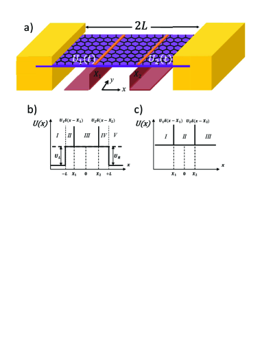
Figure 1: (Color online) a) Graphene quantum pump driven by two thin barriers imposed via two thin gates. The periodic variations of the magnitudes or positions of the thin barriers are considered as pumping parameters. b) Electrostatic potential through the system in the case of highly doped leads and (c) undoped leads. The solid lines show the instantaneous potential profile during the pumping cycle.

3 Highly doped leads

As it has been shown in the Fig. (1b), system has five regions in the case of highly doped leads. In the leads, where $U_{L,R}\rightarrow-\infty$, carriers densities are very large in contrast to the pumping region. This situation is realized by the metallic leads. The highly doped leads induce evanescent modes in the pumping region and it leads to the contribution of the evanescent modes in the pumped current. The wave functions in the left ($x<-L$) and right ($x>L$) leads are,

$$\Psi_{L}=e^{i(K_{L}x+qy)}\left(\begin{array}[]{cc}\begin{array}[]{c}1\end{array}\\ \begin{array}[]{c}1\end{array}\end{array}\right)+re^{i(-K_{L}x+qy)}\left(\begin{array}[]{cc}\begin{array}[]{c}1\end{array}\\ \begin{array}[]{c}-1\end{array}\end{array}\right),$$ (13)

$$\Psi_{R}=te^{i(K_{R}x+qy)}\left(\begin{array}[]{cc}\begin{array}[]{c}1\end{array}\\ \begin{array}[]{c}1\end{array}\end{array}\right),$$ (18)

where $r$ and $t$ are reflection and transmission coefficients, respectively. In the above relations $q$ is the transverse momentum and $K_{L,R}=\sqrt{\left(\frac{E-U_{L,R}}{\hbar v_{F}}\right)^{2}-q^{2}}$ are the wave vectors in the leads. In the pumping region, region between the left lead and first delta potential $-L<x<X_{1}$, region between two delta potentials $X_{1}<x<X_{2}$ and region between second delta potential and the right lead $X_{2}<x<L$ which are denoted by $j=1,2,3$ respectively, wave functions read

$$\Psi_{j}=a_{j}e^{i(kx+qy)}\left(\begin{array}[]{cc}\begin{array}[]{c}1\end{array}\\ \begin{array}[]{c}e^{i\phi}\end{array}\end{array}\right)+b_{j}e^{i(-kx+qy)}\left(\begin{array}[]{cc}\begin{array}[]{c}1\end{array}\\ \begin{array}[]{c}-e^{-i\phi}\end{array}\end{array}\right),$$ (27)

where $k=\sqrt{\left(\frac{E}{\hbar v_{F}}\right)^{2}-q^{2}}$ is the wave vector in the pumping region and $\phi=\tan^{-1}(\frac{q}{k})$ is the incident angle. The boundary conditions for these wave functions are the continuity at the $x=\pm L$ and satisfying the following conditions at the positions of the delta potentials

$$\Psi_{2}|_{x=X_{1}}=\mathcal{T}_{1}\Psi_{1}|_{x=X_{1}},~{}\Psi_{3}|_{x=X_{2}}=\mathcal{T}_{2}\Psi_{2}|_{x=X_{2}},$$ (28)

where

$$\mathcal{T}_{1,2}=\frac{1+i\sigma_{x}U_{1,2}/2\hbar v_{F}}{1-i\sigma_{x}U_{1,2}/2\hbar v_{F}}=e^{2i\sigma_{x}\tan^{-1}(\frac{U_{1,2}}{2\hbar v_{F}})}.$$ (29)

This boundary condition is obtained by integrating the Dirac equation through a symmetric delta function potential [35]. We obtain transmission and reflection coefficients by solving these equations. The obtained expressions are very lengthy to be given here. In the following we calculate the pumped current in the case of the highly doped leads for oscillating and vibrating thin barriers.

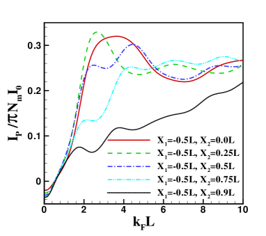
Figure 2: (Color online) Normalized pumped current as a function of the carrier concentration, $k_{F}L$, for different configurations of the oscillating thin barriers. Where we have considered $U_{1,0}=U_{2,0}=0$.

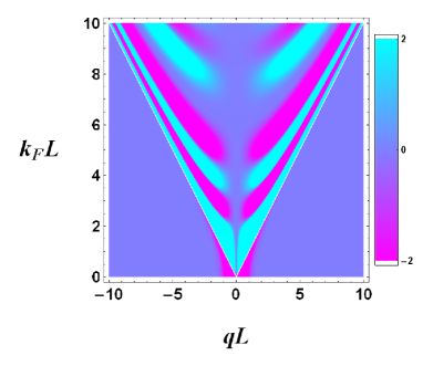
Figure 3: (Color online) Momentum distribution of the normalized pumped current as a function of the transverse momentum $q$ and the carrier concentration $k_{F}L$ in the case of the oscillating thin barriers for $U_{1,0}=U_{2,0}=0$ and $X_{2}=-X_{1}=0.5L$. The white lines indicate the points with $|q|=k_{F}$. Around the Dirac point, the evanescent modes ($|q|>k_{F}$) contribute in the pumped current in opposite direction of the extended modes ($|q|\leq k_{F}$).

3.1 Driving by the oscillating thin barriers

Let us focus to the pumped current generated by variations of the magnitudes of two thin potential barriers given by Eq. (2). In this case the pumped current is obtained by the following relation

$$I_{P}=I_{0}\sum_{n}Im\left\{\frac{\partial r}{\partial U_{1}}\frac{\partial r^{\ast}}{\partial U_{2}}+\frac{\partial t}{\partial U_{1}}\frac{\partial t^{\ast}}{\partial U_{2}}\right\},$$ (30)

where $I_{0}=(\omega/2\pi)e\delta U_{1}\delta U_{2}\sin\varphi$ and summation is over the transverse modes denoted by $n$. For short and wide graphene ($W\gg L$) we can change the summation over $n$ to integration over the continuous transverse momentum, $\sum_{q}\rightarrow(W/2\pi)\int dq$. Thus, the pumping current reads

$$I_{P}=N_{m}I_{0}\int^{+\infty}_{-\infty}\frac{dq}{k_{F}}Im\left\{\frac{\partial r}{\partial U_{1}}\frac{\partial r^{\ast}}{\partial U_{2}}+\frac{\partial t}{\partial U_{1}}\frac{\partial t^{\ast}}{\partial U_{2}}\right\},$$ (31)

where $N_{m}=4k_{F}W/\pi$ is the number of the propagating modes in the pump and $k_{F}$ is the Fermi momentum. The coefficient $4$ is due to the degeneracy including two valleys and two spin states in graphene. In Fig. (2) we have shown the normalized pumped current $I_{P}/\pi N_{m}I_{0}$, as a function of $k_{F}L$ (characterizing the carrier concentration) for different configurations of the potential barriers. These plots reveal some important features. First, the pumped current changes sign around $k_{F}L\sim 1/2$. It happens due to the generation of the pumped current by the evanescent modes ($|q|>k_{F}$) in opposite direction of the pumped current generated by the extended modes ($|q|\leq k_{F}$), around the Dirac point. To explain it, we have shown the kernel or the momentum distribution of the normalized pumped current in the Fig. 3. It shows that around the Dirac point oscillating thin barriers drive electrons occupying extended and evanescent modes in different directions. At a specific value of $k_{F}L$ these opposite contributions cancel each other and the pumped current vanishes. This feature can help to distinguish between the pumped and the rectified currents [36]. Second, minimum of the pumped current, pumped current at the Dirac point, depends on the configuration of the potential barriers and in contrast to the Ref. [24], it has not an universal value. Third, there is a weak oscillatory behavior in the curves which is caused by the quantum interferences due to the reflections from two thin potential barriers. Fourth, all of the plots tend to the same value $I_{P}/\pi N_{m}I_{0}$=0.25 in the limit of large $k_{F}L$. It happens irrespective of the pump configuration and it is identical to the result of Ref. [24].

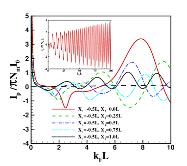
Figure 4: (Color online) Normalized pumped current as a function of the carrier concentration $k_{F}L$, for different configurations of the vibrating thin barriers. Where $U_{1}=U_{2}=\hbar v_{F}$ has been considered. Inset: Normalized pumped current as a function of the carrier concentration in the wide range of $k_{F}L$ for $X_{2}=-X_{1}=0.5L$.

3.2 Driving by the vibrating thin barriers

In this section we consider the pumped current generated by the vibration of two thin potential barriers around their equilibrium positions, given by Eq. (2). For this case the pumped current reads

$$I_{P}=N_{m}I_{0}\int^{+\infty}_{-\infty}\frac{dq}{k_{F}}Im\left\{\frac{\partial r}{\partial X_{1}}\frac{\partial r^{\ast}}{\partial X_{2}}+\frac{\partial t}{\partial X_{1}}\frac{\partial t^{\ast}}{\partial X_{2}}\right\},$$ (32)

where $I_{0}=(\omega/2\pi)e\delta X_{1}\delta X_{2}\sin\varphi$. In the calculations we consider that $U_{1}=U_{2}=\hbar v_{F}$. Fig. (4) shows the normalized pumped current as a function of $k_{F}L$. As it is apparent from the figure, there are main differences between the pumped current generated by the position and magnitude variations of the potential barriers. In the case of driving by position variation, the normalized pumped current, pumped current per mode normalized by $I_{0}$, diverges at the Dirac point. It indicates the nonzero value of the pumped current at the vanishingly small density of states around the Dirac point. The pumped current shows asymmetric oscillations around the zero as a function of the carrier concentration. For vibrating thin barriers the pumped current keeps an increasing oscillatory behavior by increasing $k_{F}L$, as it has been shown in the inset of Fig. (4). It is in contrast with the oscillating thin barriers which the pumped current tends to a limited value at large $k_{F}L$.

To clarify the obtained results, we compare the momentum distribution of the pumped current for the oscillating and vibrating thin barriers. The momentum distribution is a symmetric function of the transverse momentum $q$. Thus, it lets us to plot the momentum distributions for two different driving methods in one figure. Left half of Fig. (5) shows momentum distribution for the oscillating thin barriers and the right half of it belongs to the vibrating thin barriers for $U_{1,0}=U_{2,0}=\hbar v_{F}$ and $X_{2,0}=-X_{1,0}=0.5L$. As it is apparent in the figure, in both cases the contribution of the normal incident Dirac fermions ($q=0$) in the pumped current is zero due to the Klein tunneling. Contribution of the evanescent modes in the pumped current around the Dirac point is considerable in both cases. In spite of these similarities there is a main difference between two methods of driving. In the case of the vibrating thin barriers the contribution of the extended modes increases by increasing carrier concentration, whereas it decreases in the case of the oscillating thin barriers. This feature makes pumping by the vibrating thin barriers more effective than the oscillating ones.

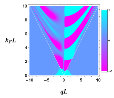
Figure 5: (Color online) Comparison of the momentum distributions of the normalized pumped currents as a function of the transverse momentum $q$ and the carrier concentration $k_{F}L$ for the oscillating (left half) and the vibrating (right half) thin barriers. Here we have considered $U_{1,0}=U_{2,0}=\hbar v_{F}$ and $X_{2,0}=-X_{1,0}=0.5L$. The white lines indicate the points with $|q|=k_{F}$.

4 Undoped leads

There are three different regions in the system with undoped leads. The region on the left of the first delta potential $x<X_{1}$, region between two delta potentials $X_{1}<x<X_{2}$ and the region on the right of the second delta potential $X_{2}<x$. The wave functions in the left and right leads are as follows

$$\Psi_{L}=e^{i(kx+qy)}\left(\begin{array}[]{cc}\begin{array}[]{c}1\end{array}\\ \begin{array}[]{c}e^{i\phi}\end{array}\end{array}\right)+re^{i(-kx+qy)}\left(\begin{array}[]{cc}\begin{array}[]{c}1\end{array}\\ \begin{array}[]{c}-e^{-i\phi}\end{array}\end{array}\right),$$ (41)

$$\Psi_{R}=te^{i(kx+qy)}\left(\begin{array}[]{cc}\begin{array}[]{c}1\end{array}\\ \begin{array}[]{c}e^{i\phi}\end{array}\end{array}\right).$$ (46)

In the pump region the wave function is

$$\Psi_{p}=ae^{i(kx+qy)}\left(\begin{array}[]{cc}\begin{array}[]{c}1\end{array}\\ \begin{array}[]{c}e^{i\phi}\end{array}\end{array}\right)+be^{i(-kx+qy)}\left(\begin{array}[]{cc}\begin{array}[]{c}1\end{array}\\ \begin{array}[]{c}-e^{-i\phi}\end{array}\end{array}\right).$$ (55)

where $k=\sqrt{\left(\frac{E}{\hbar v_{F}}\right)^{2}-q^{2}}$ is the wave vector in the pumping region as well as leads and $\phi=\tan^{-1}(\frac{q}{k})$ is the incident angle. These wave functions should satisfy the following boundary conditions

$$\Psi_{p}|_{x=X_{1}}=\mathcal{T}_{1}\Psi_{L}|_{x=X_{1}},~{}\Psi_{R}|_{x=X_{2}}=\mathcal{T}_{2}\Psi_{p}|_{x=X_{2}}.$$ (56)

$\mathcal{T}_{1,2}$ are given by the Eq. (29). Solution of these equations yields the reflection and transmission coefficients. Since, the obtained expressions are lengthy we will not give them here.

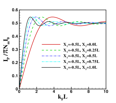
Figure 6: (Color online) Normalized pumped current as a function of the carrier concentration, $k_{F}L$, for different configurations of the oscillating thin barriers. Here $U_{1,0}=U_{2,0}=0$.

4.1 Oscillating thin barriers

In this section we present the results for the oscillating thin barriers in the case of the undoped leads. The pumped current is given by Eq. (31) and we obtain a simple analytical equation for it,

$$I_{P}=N_{m}I_{0}\int^{+\infty}_{-\infty}\frac{dq}{k_{F}}\frac{q^{2}}{k^{2}}\sin\left(2k(X_{2}-X_{1})\right).$$ (57)

As it has been shown in Fig. (6), the normalized pumped current vanishes at the Dirac point due to the absence of the extended and evanescent modes. It has an oscillatory behavior as a function of the carrier concentration arisen by quantum interferences. At large values of $k_{F}L$ the normalized pumped current tends to a limited value $I_{P}/\pi N_{m}I_{0}=0.5$, as also indicated in the Ref. [24].

4.2 Vibrating thin barriers

For the vibrating thin barriers the pumped current is given by Eq. (32). The normalized pumped current has been shown in Fig. (7) for different configurations of the pump and $U_{1}=U_{2}=\hbar v_{F}$. As it is apparent from Fig. (7), the pumped current vanishes around the Dirac point. At the Dirac point all of the modes in the pump are unpopulated and there is not nonzero contribution in the pumped current. It is due to the absence of the extended modes at the Dirac point and the evanescent modes in the graphene connected to the undoped leads. As in the case of the highly doped leads, there is an increasing oscillatory behavior in the normalized pumped current as a function of $k_{F}L$.

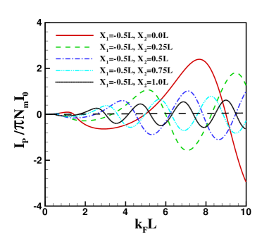
Figure 7: (Color online) Normalized pumped current as a function of the carrier concentration $k_{F}L$, for different configurations of the vibrating thin barriers. Here $U_{1}=U_{2}=\hbar v_{F}$.

5 Unique features

For emphasizing the unique feature of the pumping by vibrating thin barriers in graphene, we compare it with a similar normal pump (a similar pump based on the 2DEG). We notice that, the pumped current in graphene shows similar behaviors for large values of the carrier concentration in both cases of the highly doped and the undoped leads. Thus, we just compare the results in the case of the undoped leads. For the normal pump we should solve the Schrodinger equation in the presence of the two delta function potentials and then, mode matching gives us the reflection and the transmission coefficients. As like as graphene, the pumped current for the normal pump shows an oscillatory behavior as a function of $k_{F}L$. But, in spite of the graphene its amplitude decreases by increasing carrier concentration. To be clear, we compare the momentum distributions of the normal and graphene pumps. In Fig. (8), the left half shows momentum distribution for the normal pump and the right half belongs to the graphene pump. The oscillatory behavior in both cases is clearly apparent in the figure. But, contribution of the extended modes in the pumped current follows opposite directions by increasing the carrier concentration. It increases in the graphene pump, whereas it decreases in the normal pump. Thus, we can conclude that the increasing contribution of the extended modes in the pumped current is a unique feature for driving of the Dirac fermions by the vibrating potential barriers.

Let us to discuss the practical situations. In the case of the highly doped leads the normalized pumped current ($i_{p}=I_{P}/\pi N_{m}I_{0}$) generated by the oscillating thin barriers tends to a limited value at the Dirac point. It means that at $k_{F}L\rightarrow 0$, where the number of the extended modes $N_{m}$ vanishes, the pumped current $I_{P}$ should also vanish. On the other hand, the normalized pumped current generated by the vibrating thin barriers diverges at the dirac point. But, when $k_{F}L\rightarrow 0$ and $i_{p}\rightarrow\infty$, $k_{F}Li_{p}\sim 1$ and the pumped current tends to a nonzero value at the Dirac point. we can estimate the magnitude of the pumped current by considering an adiabatic pumping frequency in the range of the terahertz, $\omega/2\pi\sim 1.0$ THz [24]. Assuming typical values in the experiments for other parameters, $W/L\sim 10-100$, $\delta X_{1,2}/L\sim 0.01-0.1$ and $\varphi=\pi/2$, we have a pumped current around $I_{P}\sim 0.5-500$ nA. It is due to the efficient contribution of the evanescent modes in the pumped current generated by the vibrating thin barriers. This value for the pumped current at the Dirac point is well accessible in the experiment.

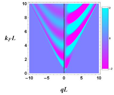
Figure 8: (Color online) Comparison of the momentum distributions of the normalized pumped currents as a function of the transverse momentum $q$ and the carrier concentration $k_{F}L$ for the normal (left half) and graphene (right half) pumps driven by vibrating thin barriers. Here we have considered $U_{1}=U_{2}=\hbar v_{F}$ and $X_{2}=-X_{1}=0.5L$.

6 Conclusion

In conclusion we have investigated a new mechanism for driving the graphene pump. In this graphene pump two thin potential barriers are employed to drive the system out of equilibrium via two different methods of magnitude oscillation and position vibration. The case of driving by oscillating thin barriers has a similarity to the graphene pump considered in the Ref. [24]. As it is expected, at the large carrier concentrations our results tend to their results. It is due to the fact that, at large carrier concentrations the exact configuration of the pump has an insignificant effect in the pumped current. But, there are important differences in vicinity of the Dirac point. The minimum of the pumped current, arising due to the contribution of the evanescent modes, depends on the pump configuration and it has not a universal value in spite of the Ref. [24]. Also, the pumped current changes sign around the Dirac point due to the opposite contributions of the evanescent and extended modes. On the other hand, new features appear in the case of the vibrating thin barriers. The pumped current has an increasing oscillatory behavior around zero as a function of the carrier concentration. It is due to the increasing contribution of the extended modes in the pumped current by increasing the carrier concentration. Comparison with the similar normal pump indicates that it is a unique feature of the Dirac fermions. Also, the normalized pumped current diverges at the Dirac point due to the more effective contribution of the evanescent modes when the thin barriers have nonzero magnitudes. Due to these facts, we can conclude that driving by oscillating and vibrating thin barriers are very effective methods to generate a pumped current in graphene. Thus, despite of the practical difficulties for experimental realization of the considered pump we believe that it has a more chance to be confirmed in the experiment.

we have considered the thin potential barriers as a delta function potentials in our calculations. It is a limited situation and in practice we expect a determinate width for the thin potential barriers. It results to a complex dependence of the pumped current on the width and height of the potential barriers. We will consider this situation in the subsequent works.

References

References

- [1] Thouless D J 1983 Phys. Rev. B 27 6083
- [2] Brouwer P W 1998 Phys. Rev. B 58 R10135
- [3] Moskalets M and Büttiker M 2002 Phys. Rev. B 66 035306
- [4] Makhlin Yu and Mirlin A D 2001 Phys. Rev. Lett. 87 276803
- [5] Zhou F Spivak B and Altshuler B 1999 Phys. Rev. Lett. 82 608
- [6] Altshuler B L and Glazman L I 1999 Science 283 1864
- [7] Das Kunal K Kim S and Mizel A 2006 Phys. Rev. Lett. 97 096602
- [8] Avishai Y Cohen D and Nagaosa N 2010 Phys. Rev. Lett. 104 196601
- [9] Wang L Troyer M and Dai X 2013 Phys. Rev. Lett. 111 026802
- [10] Switkes M Marcus C M Campman K and Gossard A C 1999 Science 283 1905
- [11] Watson S K Potok R M Marcus C M and Umansky V 2003 Phys. Rev. Lett. 91 258301
- [12] Buitelaar M R Kashcheyevs V Leek P J Talyanskii V I Smith C G Anderson D Jones G A C Wei J and Cobden D H 2008 Phys. Rev. Lett. 101 126803
- [13] Vartiainen J J Mottonen M Pekola J P and Kemppinen A 2007 Appl. Phys. Lett. 90 082102
- [14] Giazotto F Spathis P Roddaro S Biswas S Taddei F Governale M and Sorba L 2011 Nature Phys. 7 857
- [15] Novoselov K S Geim A K Morozov S V Jiang D Zhang Y Dubonos S V Grigorieva I V and Firsov A A 2004 Science 306 666
- [16] Novoselov K S Geim A K Morozov S V Jiang D Katsnelson M I Grigorieva I V Dubonos S V and Firsov A A 2005 Nature 438 197
- [17] Zhang Y Tan Y W Stormer H L and Kim P 2005 Nature 438 201
- [18] Castro Neto A H Guinea F Peres N M R Novoselov K S and Geim A K 2009 Rev. Mod. Phys. 81 109
- [19] Das Sarma S Adam S Hwang E H and Rossif E 2011 Rev. Mod. Phys. 83 407
- [20] Katsnelson M I Novoselov K S and Geim A K 2006 Nature Phys. 2 620
- [21] Tworzydlo J Trauzettel B Titov M Rycerz A and Beenakker C W J 2006 Phys. Rev. Lett. 96 246802
- [22] Gusynin V P and Sharapov S G 2005 Phys. Rev. Lett. 95 146801
- [23] Beenakker C W J 2008 Rev. Mod. Phys. 80 001337
- [24] Prada E San-Jose P and Schomerus H 2009 Phys. Rev. B 80 245414; 2011 Solid State Comm. 151 1065
- [25] Grichuk E and Manykin E 2013 Eur. Phys. J. B 86 210
- [26] Zhu R and Chen H 2009 Appl. Phys. Lett. 95 122111
- [27] Bercioux D Urban D F Romeo F and Citro R 2012 Appl. Phys. Lett. 101 122405
- [28] Low T Jiang Y Katsnelson M and Guinea F 2012 Nano Lett. 12 850
- [29] Tiwari R P and Blaauboer M 2010 Appl. Phys. Lett. 97 243112
- [30] Alos-Palop M and Blaauboer M 2011 Phys. Rev. B 84 073402
- [31] Kundu A Rao S and Saha A 2011 Phys. Rev. B 83 165451
- [32] Wakker G M M and Blaauboer M 2010 Phys. Rev. B 82 205432
- [33] San-Jose P Prada E Kohler S and Schomerus H 2011 Phys. Rev. B 84 155408
- [34] Avron J E Elgart A Graf G M and Sadun L 2000 Phys. Rev. B 62 R10618
- [35] Titov M 2007 Europhys. Lett. 79 17004
- [36] Brouwer P W 2001 Phys. Rev. B 63 121303(R)