Geometric Curvature and Phase of the Rabi model
Abstract
We study the geometric curvature and phase of the Rabi model. Under the rotating-wave approximation (RWA), we apply the gauge independent Berry curvature over a surface integral to calculate the Berry phase of the eigenstates for both single and two-qubit systems, which is found to be identical with the system of spin-1/2 particle in a magnetic field. We extend the idea to define a vacuum-induced geometric curvature when the system starts from an initial state with pure vacuum bosonic field. The induced geometric phase is related to the average photon number in a period which is possible to measure in the qubit-cavity system. We also calculate the geometric phase beyond the RWA and find an anomalous sudden change, which implies the breakdown of the adiabatic theorem and the Berry phases in an adiabatic cyclic evolution are ill-defined near the anti-crossing point in the spectrum.
keywords:
Geometric curvature and phase , Rabi model , Two-qubit1 Introduction
The Pancharatnam-Berry phase [1, 2], or most commonly known as Berry phase, has provided us a very deep insight on the geometric structure of quantum mechanics. It is worthwhile to note that Berry phase has attracted considerable interests in quantum theory on account of giving rise to interesting observable physical phenomena, implementing the operation of a universal quantum logic gate in quantum computing [3, 4, 5, 6]. The most significant characteristic for the concept of Berry phase is the existence of a continuous parameter space in which the state of the system varies slowly along a closed cycle [2, 7, 8]. In particular, various extensions of the phase have been considered [9], such as geometric phases for mixed states [10], for open systems [11], and with a quantized driving field [12, 13, 14, 15, 16, 17]. Furthermore, the concept of a geometric phase has been generalized to the case of noneigenstates, which is applicable to both linear and nonlinear quantum systems [18]. In the linear case, the geometric phase reduces to a statistical average of Berry phases for the eigenstates, weighted by the probabilities that the system finds itself in the eigenstates.
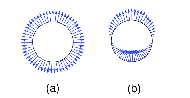
The Jaynes-Cummings (JC) model [19], or the quantum Rabi model [20] with the rotating wave approximation (RWA) that describes a spin-1/2 particle interacting with a single mode quantized field, plays an important role in the cavity quantum electrodynamics. So Fuentes-Guridi et al. [12] calculated the Berry phase of the JC model considering the quantum nature of the field. A recent work [21] made a comparison study between the Berry phases of the JC model with and without the RWA where the Berry phase for the ground state varied from zero under the RWA to nonzero values beyond the RWA. In addition, by means of two unitary transformations, the Berry phase of the JC model without the RWA, is presented in a simple and straightforward analytical method [22]. Clearly, the Berry phases mentioned above are calculated using the gauge dependent Berry connection. However, since the final result was gauge independent, there should be a gauge independent way to calculate it. This is provided by the Berry curvature that plays the role of a magnetic field in the parameter space and is a more fundamental quantity than the Berry connection. The example of spin-1/2 particle in a magnetic field is often used to demonstrates the basic concepts and important properties of the Berry phase [2, 7, 8]. The corresponding curvature in its vector form is an effective magnetic field in parameter space generated by a Dirac magnetic monopole of strength in the origin as shown in Fig. 1(a), where we present the cross section for the field distribution on the surface of a unit sphere. Obviously, it is homogeneous and isotropic in parameter space. Berry phase can then be interpreted as the magnetic flux through the area whose boundary is the closed loop. It only depends on the global property of the adiabatic evolutions, which offers potential advantages against local fluctuations for implementing geometric quantum gates [23]. Motivated by this application of Berry phase in phase-shift gate operation in quantum computation [3, 4, 5, 6], we investigate the effect of the geometric phase of the Rabi model from the viewpoint of geometric connection and curvature.
In this paper we calculate the geometric phase of the two-qubit Rabi model where two qubits interact with the quantized field inhomogeneously. In Sec II we first review the analytical results for eigen solutions of the two-qubit Rabi model with the RWA according to the conservation of total number of excitation and present the analytical expressions of the Berry phase for the eigenstates. The procedure is as follows: From the connection we derive the curvature, the integration of which gives the phase. Then we turn to the geometric curvature and phase for noneigenstates in order to tackle the pure geometric effect induced by the vacuum photon state. The system returns back to its initial state after a period, which realizes a vacuum-to-vacuum cyclic evolution. We analyze the corresponding geometric curvature field, in comparison with the example of spin- particle. In Sec. III we study the Berry phase of the two-qubit Rabi model beyond the RWA. The adiabatic approximation is adopted to derive the analytical results for Berry phases of the eigenstates. For strong coupling case we truncate the Hilbert space and calculate the phases numerically. The geometric phases for the evolution of noneigenstates are compared with and without the RWA. Sec. IV summarizes our main findings.
2 Geometric phase under the RWA
2.1 Berry phase for eigenstates
The two-qubit Rabi model is described by the Hamiltonian () [20]
| (1) |
Here () is the bosonic creation (annihilation) operator of field mode with frequency , and denotes the energy splitting of qubit described by Pauli matrices and . We notice that the dipole-field coupling strength are not necessarily the same for the two qubits, rendering a typical inhomogeneously coupled system.
One convenient way to handle the Hamiltonian is the RWA where the counter-rotating terms are neglected in the weak coupling case. We begin with the simplest case with and , in which case the Hamiltonian (1) is simplified to the JC model with eigenvalues
| (2) |
where denotes the total excitations of the qubit and the photons, the Rabi frequencies , and the detuning . Its eigenstates are
| (3) |
where , and are respectively the upper and lower eigenstates of , and is photon number state.
The Berry phase is known as a geometric effect when the wave function of the system undergoes adiabatic evolution along a closed curve in the parameter space [2]. The phase change in the coupled state of qubits and field is generated by introducing the phase shift operator , which is applied adiabatically to the Hamiltonian of the system, i.e. . In the simplest case, where the detuning and coupling strength are fixed and the phase is varied slowly from to , each eigenstate of the system undergoes a closed loop on the Bloch sphere and the Berry phase induced in this way is calculated as
| (4) |
For the eigenstates (3) we easily obtain
| (5) |
For the two-qubit Rabi model (1), we use the eigenstates of the free qubits and free field as basis vectors and treat the Hamiltonian in the Hilbert space
| (6) |
The product states of two qubits are defined as , , , . The space is shared with the operator , which again counts the total excitations of the qubits and the photons. Denote the eigenvalues of as , which can be used as quantum number to classify the energy eigenstates. This leads immediately to a decomposition of the system Hilbert space into subspaces, i.e. with
| (7) |
We note that except the state , the subspace is three-fold degenerate for , and four-fold degenerate for . The fact that commutes makes it true that the subspace is invariant under , and the matrix representation of takes a block diagonal form with
| (9) | |||||
| (13) |
and
| (19) | |||||
with the identity matrix. The eigenstates can be solved by diagonalizing the matrices in associated subspaces as
| (20) |
where labels the different eigenstates with any given ( with and with ). Substituting the expression of into Eq. (4), we obtain the Berry phases for the eigenstates of two-qubit Rabi model
| (21) |
where , with and is the sign function.
The coefficients of the eigenstates are tedious algebraic functions of system parameters and . As an example, in the case of , the eigenvalues for can be expressed as
| (22) |
with . We find , and the three eigenstates with can be simplified as
| (23) |
where and are the eigenstates of the uncoupled system and expressed as
| (24) |
with . Furthermore, the corresponding Berry phases are respectively
| (25) |
Here we discuss some features of the Berry phases for some exceptional eigenstates of the system. First, similar to the case of JC model, the vacuum state is the real ground state with energy and the corresponding Berry phase is trivially zero. Second, in the case of and , it is easy to show that the eigenstate acquires no geometric phase, too. These two eigenstates share a common feature that only vacuum state of the bose field is involved. Finally, for two identical qubits and , the spin singlet states (for any ) are eigenstates of the system. The corresponding Berry phases are integer multiples of , which would not affect the wave functions. The resultant phases for the eigenstates other than the above-mentioned three exceptional cases are generally non-zero, which are attributed to the interaction between the qubits and the bosonic field.
2.2 Berry curvature for eigenstates
The eigenstates Eq. (3) are similar to those of a spin- particle in an external magnetic field, which describes a number of physical systems in condensed matter physics [8]. To better understand the geometric properties of the parameter space, we describe the Berry phase of the JC model in an alternative way. First we define the Berry connection or the Berry vector potential as
| (26) |
where is the eigenstate of the system that depends on time through a set of parameters denoted by . For the JC model, the parameter space is spanned by and and the Berry connection is calculated for the eigenstates as and , , which is obviously gauge dependent. It is thus useful to define a gauge-field tensor, known as the Berry curvature which can be derived from the Berry vector potential
| (27) |
It provides a local description of the geometric properties of the parameter space. The Berry curvature is gauge invariant and thus observable. It is a more fundamental quantity than the Berry phase, just as has been shown in Refs. [24, 25] that the Berry curvature directly participates in the dynamics of the adiabatic parameters and the orbital magnetization contains a Berry curvature contribution of topological origin. For the two eigenstates we have . According to Stokes’ theorem the Berry phase is the integral of the curvature on the surface enclosed by the loop on the Bloch sphere, i.e.
| (28) |
which reproduces the result Eq. (5).
One may on the other hand parametrize the parameter space in the spherical coordinates and , in which case the Berry curvature can be recast into a vector form
| (29) |
which can be viewed as an effective magnetic field in the parameter space. The result for the eigenstate is
| (30) |
where the polar angle varies from to for and from to for , and the radius changes with the coupling strength . When the field is mapped onto the unit sphere, the curvature for the JC model is isotropic just as in the example of spin- particle, which is recognized as a magnetic field generated by a monopole at the origin as shown in Fig. 1(a) [8]. The direction of the Berry curvature field for the eigenstate is opposite to the field .
The Berry connection and the Berry curvature for the two-qubit Rabi model can be calculated in the same way by mapping the parameter space into the model of spin- particle. For the three eigenstates (23) with the Berry connection as a function of and is and . The Berry curvature can be derived easily as , and , from which one can easily recover the Berry phase in Eq. (25). In spherical coordinates the Berry curvature for the eigenstate takes the same form as Eq. (30) with, however, the radius replaced by . The Berry curvatures for the eigenstates and thus show exactly the same structures as those for the eigenstates and of the JC model, respectively. However, the Berry curvature for the eigenstate is constantly zero in the whole unit sphere because only vacuum state of the bose field is involved.
2.3 Geometric curvature and phase for noneigenstates
We now turn to the geometric curvature and phase for noneigenstates of the JC model in order to tackle the pure geometric effect induced by the vacuum photon state. Staring from the initial state with a qubit in the excited state and field in the vacuum state , which happens to be a superposition of two eigenstates of the JC model
| (31) |
the time-dependent state after an adiabatic and cyclic evolution is shown to be [26]
| (32) | |||||
where and with . The evolution of the noneigenstate exhibits clear recurrence behavior with a period , that is, the state returns back to the initial state at subsequent time () with an additional phase factor, . This is a beautiful realization of the vacuum-to-vacuum evolution. Remove the dynamic part from the total phase , the Aharonov-Anandan phase (AA) phase of the evolution is obtained as [26]
| (33) |
It was found that the average photon number of the state in a period is related to the Berry phases by
| (34) | |||||
Here we discuss the geometric phase for the adiabatic and cyclic evolution of noneigenstates according to a formal definition given by Wu et al. [18]. For the linear systems, it is defined as a statistical average of Berry phases for the eigenstates, weighted by the probabilities that the system finds itself in the eigenstates
| (35) |
Interestingly, this kind of weighted summation of Berry phases has already been applied in real physical systems [27, 28]. Our scheme is based on Eq. (35) and we define the geometric connection for noneigenstates as
| (36) |
We find for noneigenstate , this connection is and the corresponding geometric curvature is calculated from the definition (27) as
| (37) |
Based on the fact that the adiabatic evolution of noneigenstate forms a closed loop in the parameter space at time , the integral of the curvature Eq. (28) on the surface defines a new geometric phase , the result for state being just the same as Eq. (35)
| (38) |
We conclude that while the AA phase describes the pure geometric phase acquired in the cyclic evolution, the geometric phase is related to the average photon number through
| (39) |
Obviously, the value of can not exceed , i.e., because the total excitations of the qubit and the photon is a conserved quantity with in the process of time evolution. It is more intuitive to consider the geometric curvature (37) in the spherical coordinates
| (40) |
which acquires an additional polar angle dependent factor . The distribution of the geometric curvature for the noneigenstate is shown in Fig. 1(b) and we find the curvature is rotationally symmetric about -axis. Interestingly, while the curvature is still centrifugal in the northern hemisphere, the factor reverses the direction of the field in the southern hemisphere and the corresponding geometric curvature field is opposite to the direction of the radius . This can be recognized as a statistical average of the magnetic field generated simultaneously by two monopoles with opposite magnetic charges. The maximum field strength lies in the north and south poles, which is chosen as the reference and set to be unity, while on the equator the field is zero.
For the two-qubit Rabi model, the initial state with the field in the vacuum state can be expressed as a superposition of eigenstates of the system
| (41) |
with
| (42) |
The time-dependent state after an adiabatic and cyclic evolution is similar to the case of JC model [26]
| (43) |
where the instantaneous eiegnstates are and the corresponding eiegnenergies are
| (44) |
Consider for example the special case of , the eigenenergies and eigenstates of which are given by the Eqs. (22) and (23) in the previous section. Interestingly, if the ratio of the two eigenvalues is a rational number
| (45) |
where and are integers, at subsequent time the noneigenstate returns back to the initial state with an additional phase factor , i.e. . In a recent work [29] Ballester et al. introduced an effective qubit-cavity system tuning the parameters of the external drivings, where the frequency is in a magnitude of MHz and in near resonance with the frequency of the qubit in the strong driving limit. For example, for a detuning and weak coupling , we have and . This is the vacuum-to-vacuum evolution in the two-qubit case and the geometric phase in the evolution is induced by pure vacuum state of photons. The AA phase in the evolution is again obtained by removing the dynamical phase from
| (46) |
The connection for the state is , from which the geometric curvature is obtained as
| (47) |
The geometric phase is derived by a surface integral according to Eq. (28)
| (48) |
and related to the AA phase through
| (49) |
The vacuum induced geometric phase is again related to the average photon number in a period through Eq. (39) and thus can be measured by counting the photons during the cyclic evolution. The average photon number in the two-qubit model is limited to a maximum value which depends on the ratio of the coupling strength . For homogeneous coupling , we find . The geometric curvature in the spherical coordinates
| (50) |
shows exactly the same distribution in the parameter space as the single qubit case in Fig. 1(b) once we set the maximum field strength to be unity.
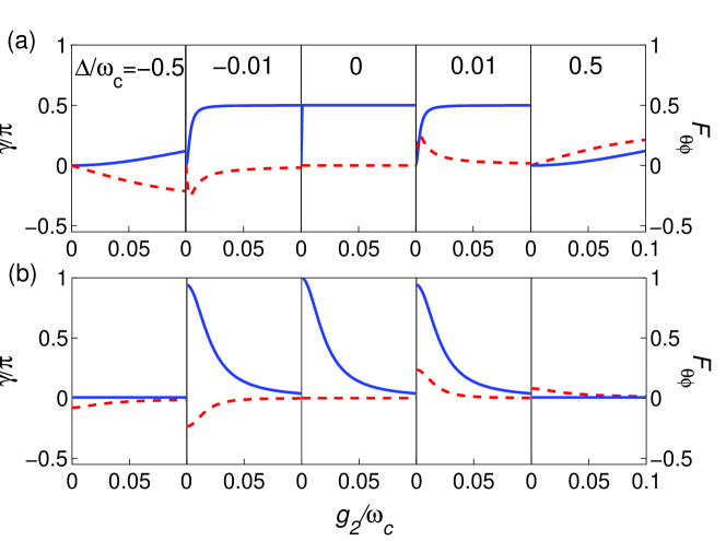
We illustrate in Fig. 2 the geometric curvature in (47) and the geometric phase in (48) as a function of the coupling strength for an adiabatic and cyclic evolution of the initial state . Several typical detuning cases are shown for homogeneous and inhomogeneous coupling systems. While the geometric phases are always positive definite, the respective geometric curvatures are of opposite sign for red and blue detunings, as can be seen from Fig 1(b). For homogeneous coupling case, while increases gradually with the coupling strength in the case of far off-resonant interaction, it reaches the maximum value very quickly near the resonance. The geometric curvature, on the other hand, develops a peak or a valley for small detuning at , though it depends on monotonically for large ones. For inhomogeneous coupling shown in Fig. 2(b), the maximum geometric phase acquired in the evolution is , which occurs in the single qubit system for exact resonant condition. The phase and curvature are suppressed to nearly zero for non-equal coupling strengths, corresponding to the circle on the equator in Fig 1(b).
Experiments have shown that many engineering systems enable us to access coupling strengths and detunings outside the regime in which the RWA is valid, such as circuit QED experiments with superconducting qubits coupled to LC and waveguide resonators [30, 31, 32, 33] and Cooper-pair boxes or Josephson phase qubits coupled to nanomechanical resonators [34, 35, 36, 37, 38]. In next section we study the Berry phase beyond the RWA, which shows very different feature from the RWA results.
3 Berry phase beyond the RWA
The Hamiltonian for the two-qubit Rabi model beyond the RWA fails to commute with the total excitation operator and the block diagonal form of the matrix breaks down. One would conclude that the appearance of the counter-rotating terms makes it impossible to solve the Hamiltonian exactly. However, the employment of Bargman-space technique, or displaced Fock state provides a way to solve the model analytically [39, 40, 41, 42]. The adiabatic approximation proves to be an excellent way to treat the eigenenergies when the transition frequency of the qubit is much smaller than the frequency of bose field and the coupling strength enters into the ultrastrong coupling regime. The eigenstates under this approximation have the form
| (51) |
which are expanded in the displaced Fock state basis . Here labels the parity, the displaced Fock states are defined as with , and and . The coefficients in Eq. (51) are
with
We find the corresponding eigenergies for the analytical eigenstates (51) are expressed as
| (52) |
and the corresponding Berry phases are calculated as
| (53) |
with , which are accurate in the weak coupling case with up to . For even stronger coupling we resort to numerical scheme described as following. The eigenstates are expanded in the truncated displaced Fock space as
| (54) | |||||
and the Berry phase for eigenstates is by definition (4) calculated as
| (55) | |||||
Here the coefficients ’s are obtained numerically by setting the truncation number as such that the calculation is done in a closed subspace with .
Before we present the numerical results for the Berry phase of the eigenstates, we first give the result for the exceptional spectrum of the two-qubit model. First, the spin singlet state for two identical qubits remains eigenstate of the system beyond the RWA, which acquires a geometric phase as in RWA. In addition, in the homogeneous coupling case , there exists a constant analytical solution [41, 42] corresponding to either the even parity eigenstate
for the symmetric detuning with (suppose ), or the odd parity eigenstate
for the asymmetric detuning with and . These two states contain at most one photon and we have an exact result for their Berry phases as
| (56) |
where . Both the vacuum state and the one-photon state of the quantized field are involved in , which is analogous to the Berry phase for the eigenstates (3) and (23) for .
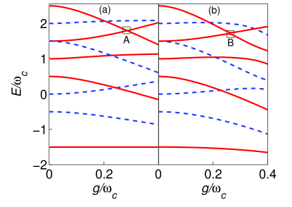
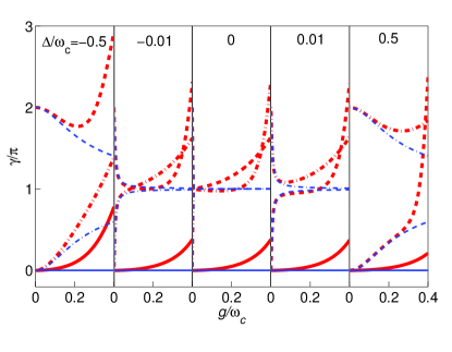
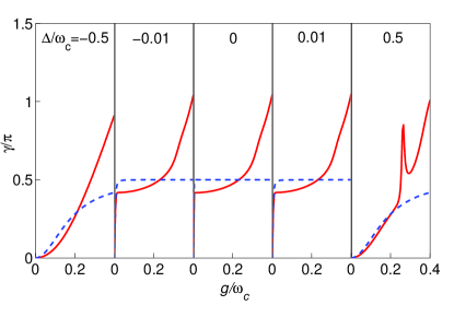
We illustrate in Fig. 3 the first few eigenergies of the homogeneously coupling system with and without the RWA as a function of coupling strength in the even and odd parity subspaces, where the eigenenergies corresponding to the spin singlet states are not shown. Particularly we have marked a crossing point (A) of energy levels for different values of in RWA and an anti-crossing point (B) within the even parity subspace beyond RWA. It is easily show that during the adiabatic evolution the quantum transition between different subspace is forbidden in RWA, i.e. . The degeneracy at (A) thus would not affect the calculation of the Berry phases. The nearly degeneracy at the anti-crossing point (B) beyond RWA, on the other hand, will break the validity of the adiabatic theorem as the transition between states in the same parity space (in the case shown in Fig. 3(b), the even parity space) is not negligible, and the condition for the adiabatic approximation is not applicable. We shall see below that these anti-crossing points lead to nontrivial contribution in the geometric phase. It demonstrates that the RWA indeed only works well in the weak coupling regime and the counterpart of the real ground state energy is not any more a constant beyond RWA. We choose to compare the Berry phases for three eigenstates in RWA and the corresponding numerical eigenstates beyond RWA in Fig. 4, the eigenenergies of which are just the lowest solid (red) and the two lowest dashed (blue) lines for the detuning in Fig. 3. Clearly the values of Berry phases under the RWA are close to those beyond the RWA in the weak coupling region. We find that in RWA the berry phase for is constantly zero, while those for and swap their positions if the detuning reverses its sign. In strong coupling regime all states acquire a much bigger Berry phase than in RWA, in some cases even exceeding .
In Fig. 5, we further compare the geometric phase for the evolution of noneigenstate in these two cases. It is shown that all geometric phases tend to a constant with the increase of the coupling strength in the RWA and are symmetric for blue and red detunings. The symmetry is broken beyond the RWA and we find an anomalous sudden change for around . We attribute this to the generic level anti-crossing in the same parity subspace in Fig. 3(b). The geometric phase of the noneigenstate here is the weighted summation of the Berry phases (55) of all eigenstates in the numerically truncated space. The transition between the two nearly degenerate eigenstates at point (B) in Fig. 3(b) in the same parity can not be neglected and the Berry phase in an adiabatic cyclic evolution is ill defined. The geometric phase is no longer applicable whenever the level anti-crossing in the same parity subspace occurs under some parameter conditions.
4 Conclusion
To conclude, we have investigated theoretically the geometric curvature and phase of the quantum Rabi model. When the wave function of the system undergoes an adiabatic evolution along a closed curve in the parameter space, we derived the analytical expressions of the Berry phase of the eigenstates under the RWA for the single- and two-qubit systems. We introduced the Berry connection and curvature to study the geometric properties of the Rabi model and it was found that the curvatures for both single- and two-qubit models are identical to the example of spin-1/2 particle. This idea is generalized to describe the vacuum-induced geometric curvature when the system starts from an initial state with pure vacuum bosonic field, which can be recognized as a statistical average of the magnetic field generated simultaneously by two monopoles with opposite magnetic charges. The induced geometric phase is related to the average photon number in a period, which is different from the AA phase of the evolution. With the displaced Fock state technique we managed to evaluate the Berry phase for eigenstates and the geometric phase for pure vacuum initial state beyond the RWA. The anti-crossing points in the spectrum invalidate the condition of the adiabatic theorem as the transition between the states in the same parity space is not negligible - an anomalous sudden change occurs in the geometric phase, which implies that the Berry phases of the eigenstates in an adiabatic cyclic evolution are ill-defined near these nearly degenerate points.
When the two-qubit system undergoes a cyclic evolution, the time dependent eigenstates will pick up Berry phases, which defines an adiabatic geometric phase gate acting on the two-qubit basis states as well as their superpositions. As an example of this, Jones et al. [6] performed an experimental realization of a controlled phase shift gate by considering an ensemble of spin half particles in a magnetic field, in which the fidelity that measures the precision of the experimentally implemented gates with respect to an ideal one was higher than traditional dynamical gates. Crucially, we have studied the Berry phase of the single- and two-qubit Rabi model, where a single quantized mode of the field is considered and the phases depend on the detuning and coupling strength . In experiment, it is easy to control the detuning and the coupling quite precisely. Therefore, the result here would be useful in the realization of geometric phase gates in a circuit QED system on the basis of similar theories. In particular, we should be more careful when considering two-qubit quantum logic gates in many experimental implementations based on the geometric phase of the model where employment of the RWA might impart incorrect results [5, 4]. Traditionally the validity of the RWA is guaranteed by the energy conservation and the weak coupling in the system. This study shows that the breakdown of the RWA also implies deviation of the geometric property of the state evolution from the true strong coupling system.
Acknowledgements
This work is supported by NSF of China under Grant Nos. 11234008 and 11474189, the National Basic Research Program of China (973 Program) under Grant No. 2011CB921601, Program for Changjiang Scholars and Innovative Research Team in University (PCSIRT)(No. IRT13076).
References
- [1] S. Pancharatnam, Proc. Indian Acad. Sci. A 44, 247 (1956).
- [2] M. V. Berry, Proc. R. Soc. London A 392, 45 (1984).
- [3] A. Nazir, T. P. Spiller, and W. J. Munro, Phys. Rev. A 65, 042303 (2002).
- [4] K. Kim, C. F. Roos, L. Aolita, H. Häfner, V. Nebendahl, and R. Blatt, Phys. Rev. A 77, 050303(R) (2008).
- [5] D. Leibfried et al., Nature 422, 412 (2003).
- [6] J. A. Jones, V. Vedral, A. Ekert, and G. Castagnoli, Nature 403, 869 (2000).
- [7] B. R. Holstein, Am, J. Phys. 57, 1079 (1989).
- [8] D. Xiao, M.-C. Chang, and Q. Niu, Rev. Mod. Phys. 82, 1959 (2010).
- [9] X.-X. Yi, L. C. Wang, and T. Y. Zheng, Phys. Rev. Lett. 92, 150406 (2004).
- [10] E. Sjöqvist et al., Phys. Rev. Lett. 85, 2845 (2000); R. Bhandari, Phys. Rev. Lett. 89, 268901 (2002); J. Anandan et al., Phys. Rev. Lett. 89, 268902 (2002).
- [11] A. Carollo, I. Fuentes-Guridi, M. Franca Santos, and V. Vedral, Phys. Rev. Lett. 90, 160402 (2003); R. S. Whituey, Y. Gefen, Phys. Rev. Lett. 90, 190402 (2003).
- [12] I. Fuentes-Guridi, A. Carollo, S. Bose, and V. Vedral, Phys. Rev. Lett. 89, 220404 (2002).
- [13] S. P. Bu, G. F. Zhang, J. Liu and Z. Y. Chen, Phys. Scr. 78, 065008 (2008).
- [14] G. Chen, J. Q. Li, and J. Q. Liang, Phys. Rev. A 74, 054101 (2006).
- [15] J. Larson, Phys. Rev. Lett. 108, 033601 (2012).
- [16] J. Larson, Phys. Scr. T 153, 014040 (2013).
- [17] E. M. Martínez, A. Dragan, R. B. Mann, I. Fuentes, New J. Phys. 15 053036 (2013).
- [18] B. Wu, J. Liu, and Q. Niu, Phys. Rev. Lett. 94, 140402 (2005).
- [19] E. T. Jaynes, and F. W. Cummings, Proc. IEEE 51, 89 (1963).
- [20] I. I. Rabi, Phys. Rev. 49, 324 (1936); 51, 652 (1937).
- [21] T. Liu, M. Feng, and K. L. Wang, Phys. Rev. A 84, 062109 (2011).
- [22] W. W. Deng, G. X. Li, J. Phys. B: At. Mol. Opt. Phys. 46, 224018 (2013).
- [23] E. Sjöqvist, Physics 1, 35 (2008).
- [24] H. Kuratsuji, and S. Iida, Prog. Theo. Phys. 74, 439 (1985).
- [25] J. Shi, G. Vignale, D. Xiao, and Q. Niu, Phys. Rev. Lett. 99, 197202 (2007).
- [26] M. H. Wang, L. F. Wei, and J. Q. Liang, Mod. Phys. Lett. B 29, 1550043 (2015).
- [27] D. J. Thouless, P. Ao, and Q. Niu, Phys. Rev. Lett. 76, 3758 (1996).
- [28] Y. G. Yao et al., Phys. Rev. Lett. 92, 037204 (2004).
- [29] D. Ballester, G. Romero, G. G. García-Ripoll, F. Deppe and E. Solano, Phys. Rev. X 2, 021007 (2012).
- [30] D. I. Schuster A. A. Houck, J. A. Schreier, A. Wallraff, J. M. Gambetta, A. Blais, L. Frunzio, J. Majer, B. Johnson, M. H. Devoret, S. M. Girvin, and R. J. Schoelkopf, Nature (London) 445, 515 (2007).
- [31] P. Forn-Díaz, J. Lisenfeld, D. Marcos, J. J. Garc ía-Ripoll, E. Solano, C. J. P. M. Harmans, and J. E. Mooij, Phys. Rev. Lett. 105, 237001 (2010).
- [32] T. Niemczyk, F. Deppe, H. Huebl, E. P. Menzel, F. Hocke, M. J. Schwarz, J. J. Garcia-Ripoll, D. Zueco, T. Hummer, E. Solano, A. Marx, and R. Gross, Nat. Phys. 6, 772 (2010).
- [33] A. A. Abdumalikov, O. Astafiev, Y. Nakamura, Y. A. Pashkin, and J. S. Tsai, Phys. Rev. B 78, 180502(R) (2008).
- [34] V. Bouchiat, D. Vion, P. Joyez, D. Esteve, and M. H. Devoret, Phys. Scri. T76, 165 (1998).
- [35] Y. Nakamura, Y. A. Pashkin, and J. S. Tsai, Nature 398, 786 (1999).
- [36] A. Wallraff, D. I. Schuster, A. Blais, L. Frunzio, R.- S. Huang, J. Majer, S. Kumar, S. M. Girvin, and R. J. Schoelkopf, Nature 431, 162 (2004).
- [37] M. Hofheinz, H. Wang, M. Ansmann, R. C. Bialczak, E. Lucero, M. Neeley, A. D. O’Connell, D. Sank, J. Wenner, J. M. Martinis, and A. N. Cleland, Nature 459, 546 (2009).
- [38] M. D. LaHaye, J. Suh, P. M. Echternach, K. C. Schwab, and M. L. Roukes, Nature 459, 960 (2009).
- [39] M. X. Liu, Z. J. Ying, J. H. An, H. G. Luo, New J. Phys. 17 043001 (2015).
- [40] S. He, L. W. Duan, Q. H. Chen, New J. Phys. 17, 043033 (2015).
- [41] J. Peng, Z. Ren, D. Braak, G. Guo, G. Ju, X. Zhang, and X. Guo J. Phys. A: Math. Theor. 47, 265303 (2014).
- [42] L. Mao, S. Huai, and Y. Zhang, J. Phys. A: Math. Theor. 48, 345302 (2015).