Optimizing Spread of Influence in Weighted Social Networks via Partial Incentives

Abstract

A widely studied process of influence diffusion in social networks posits that the dynamics of influence diffusion evolves as follows: Given a graph $G=(V,E)$, representing the network, initially only the members of a given $S\subseteq V$ are influenced; subsequently, at each round, the set of influenced nodes is augmented by all the nodes in the network that have a sufficiently large number of already influenced neighbors. The general problem is to find a small initial set of nodes that influences the whole network. In this paper we extend the previously described basic model in the following ways: firstly, we assume that there are non negative values $c(v)$ associated to each node $v\in V$, measuring how much it costs to initially influence node $v$, and the algorithmic problem is to find a set of nodes of minimum total cost that influences the whole network; successively, we study the consequences of giving incentives to member of the networks, and we quantify how this affects (i.e., reduces) the total costs of starting process that influences the whole network. For the two above problems we provide both hardness and algorithmic results. We also experimentally validate our algorithms via extensive simulations on real life networks.

Keywords: Social Networks; Spread of Influence; Viral Marketing

1 Introduction

Social influence is the process by which individuals adjust their opinions, revise their beliefs, or change their behaviors as a result of interactions with other people. It has not escaped the attention of advertisers that the natural human tendency to conform can be exploited in viral marketing [30]. Viral marketing refers to the spread of information about products and behaviors, and their adoption by people. For what strictly concerns us, the intent of maximizing the spread of viral information across a network naturally suggests many interesting optimization problems. Some of them were first articulated in the seminal papers [27, 28], under various adoption paradigms. The recent monograph [8] contains an excellent description of the area. In the next section, we will explain and motivate our model of information diffusion, state the problems that we plan to investigate, describe our results, and discuss how they relate to the existing literature.

1.1 The Model

Let $G=(V,E)$ be a graph modeling a social network. We denote by $\Gamma_{G}(v)=\{u\in V:(v,u)\in E\}$ and by $d_{G}(v)=|\Gamma_{G}(v)|,$ respectively, the neighborhood and the degree of vertex $v$ in $G$. Let $S\subseteq V$, and let $t:V\to{\mathbb{N}}=\{1,2,\ldots\}$ be a function assigning integer thresholds to the vertices of $G$; we assume w.l.o.g. that $1\leq t(u)\leq d(u)$ holds for all $v\in V$. For each node $v\in V$, the value $t(v)$ quantifies how hard it is to influence node $v$, in the sense that easy-to-influence elements of the network have “low” $t(\cdot)$ values, and hard-to-influence elements have “high” $t(\cdot)$ values [25]. An activation process in $G$ starting at $S\subseteq V$ is a sequence

$${{\sf Active}}_{G}[S,0]\subseteq{{\sf Active}}_{G}[S,1]\subseteq\ldots\subseteq{{\sf Active}}_{G}[S,\ell]\subseteq\ldots\subseteq V$$

of vertex subsets, with ${{\sf Active}}_{G}[S,0]=S$, and such that for all $\ell>0$,

$${{\sf Active}}_{G}[S,\ell]={{\sf Active}}_{G}[S,\ell-1]\cup\Big{\{}u\,:\,\big{|}\Gamma_{G}(u)\cap{{\sf Active}}_{G}[S,\ell-1]\big{|}\geq t(u)\Big{\}}.$$

In words, at each round $\ell$ the set of active (i.e, influenced) nodes is augmented by the set of nodes $u$ that have a number of already activated neighbors greater or equal to $u$’s threshold $t(u)$. We say that $v$ is activated at round $\ell>0$ if $v\in{{\sf Active}}_{G}[S,\ell]-{{\sf Active}}_{G}[S,\ell-1]$. A target set for $G$ is a set $S$ that will activate the whole network, that is, ${{\sf Active}}_{G}[S,\ell]=V$, for some $\ell\geq 0$. The classical Target Set Selection (TSS) problem (see e.g. [1, 15]) is defined as follows:

Target Set Selection.

Instance: A network $G=(V,E)$ with thresholds $t:V\longrightarrow\mathbb{N}$.

Problem: Find a target set $S\subseteq V$ of minimum size for $G$.

The TSS Problem has roots in the general study of the spread of influence in Social Networks (see [14, 8, 21]). For instance, in the area of viral marketing [20], companies wanting to promote products or behaviors might initially try to target and convince a set of individuals (by offering free copies of the products or some equivalent monetary rewards) who, by word-of-mouth, can successively trigger a cascade of influence in the network leading to an adoption of the products by a much larger number of individuals. In order to make the model more realistic, we extend the previously described basic model in two ways: First, we assume that there are non negative values $c(v)$ associated to each vertex $v\in V$, measuring how much it costs to initially convince the member $v$ of the network to endorse a given product/behavior. Indeed, that different members of the network have different activation costs (see [2], for example) is justified by the observation that celebrities or public figures can charge more for their endorsements of products. Therefore, we are lead to our first extension of the TSS problem:

Weighted Target Set Selection (WTSS).

Instance: A network $G=(V,E)$, thresholds $t:V\to\mathbb{N}$, costs $c:V\to\mathbb{N}$.

Problem: Find a target set $S\subseteq V$ of minimum cost ${C}(S)=\sum_{v\in S}c(v)$

among all target sets for $G$.

Our second, and more technically challenging, extension of the classical TSS problem is inspired by the recent interesting paper [19]. In that paper the authors observed that the basic model misses a crucial feature of practical applications since it forces the optimizer to make a binary choice of either zero or complete influence on each individual (for example, either not offering or offering a free copy of the product to individuals in order to initially convince them to adopt the product and influence their friends about it). In realistic scenarios, there could be more reasonable and effective options. For example, a company promoting a new product may find that offering for free ten copies of a product is far less effective than offering a discount of ten percent to a hundred of people. Therefore, we formulate our second extension of the basic model as follows.

Targeting with Partial Incentives. An assignment of partial incentives to the vertices of a network $G=(V,E)$, with $V=\{v_{1},\ldots,v_{n}\}$, is a vector ${\bf s}=(s(v_{1}),\dots,s(v_{n}))$, where $s(v)\in{\mathbb{N}}_{0}=\{0,1,2,\ldots\}$ represents the amount of influence we initially apply on $v\in V$. The effect of applying incentive $s(v)$ on node $v$ is to decrease its threshold, i.e., to make individual $v$ more susceptible to future influence. It is clear that to start the process, there should be a sufficient number of nodes $v$’s to which the amount of exercised influence $s(v)$ is at least equal to their thresholds $t(v)$. Therefore, an activation process in $G$ starting with incentives whose values are given by the vector ${\bf s}$ is a sequence of vertex subsets

$${{\sf Active}}[{\bf s},0]\subseteq{{\sf Active}}[{\bf s},1]\subseteq\ldots\subseteq{{\sf Active}}[{\bf s},\ell]\subseteq\ldots\subseteq V,$$

with ${{\sf Active}}[{\bf s},0]=\{v\ |\ s(v)\geq t(v)\}$, and such that for all $\ell>0$,

$${{\sf Active}}[{\bf s},\ell]={{\sf Active}}[{\bf s},\ell-1]\cup\Big{\{}u\,:\,\big{|}\Gamma_{G}(u)\cap{{\sf Active}}[{\bf s},\ell-1]\big{|}\geq t(u)-s(u)\Big{\}}.$$

A target vector ${\bf s}$ is an assignment of partial incentives that triggers an activation process influencing the whole network, that is, such that ${{\sf Active}}[{\bf s},\ell]=V$ for some $\ell\geq 0$. The Targeting with Partial Incentive problem can be defined as follows:

Targeting with Partial Incentives (TPI).

Instance: A network $G=(V,E)$, thresholds $t:V\longrightarrow\mathbb{N}$.

Problem: Find target vector ${\bf s}$ which minimizes $C({\bf s})=\sum_{v\in V}s(v)$.

Notice that the Weighted Target Set Selection problem, when the costs $c(v)$ are always equal to the thresholds $t(v)$, for each $v\in V$, can be seen as a particular case of Targeting with Partial Incentives in which the incentives $s(v)$ are set either to $0$ or to $t(v)$. Therefore, in a certain sense, the Targeting with Partial Incentives can be seen as a kind of “fractional” counterpart of the Weighted Target Set Selection problem (notice, however, that the incentives $s(v)$ are integer as well). In general, the two optimization problems are quite different since arbitrarily large gaps are possible between the costs of the solutions of the WTSS and TPI problems, as the following example shows.

Example 1.

Consider the complete graph on $n$ vertices $v_{1},\ldots,v_{n}$, with thresholds $t(v_{1})=\ldots=t(v_{n-2})=1$, $t(v_{n-1})=t(v_{n})=n-1$ and costs equal to the thresholds. An optimal solution to the WTSS problem consists of either vertex $v_{n-1}$ or vertex $v_{n}$, hence of total cost equal to $n-1.$ On the other hand, if partial incentives are possible one can assign incentives $s(v_{1})=s(v_{n})=1$ and $s(v_{i})=0$ for $i=2,\ldots,n-1$, and have an optimal solution of value equal to 2. Indeed, we have

• ${{\sf Active}}[{\bf s},0]=\{v_{1}\}$, since $t(v_{1})=s(v_{1})$,

• ${{\sf Active}}[{\bf s},1]=\{v_{1},v_{2},\ldots,v_{n-2}\}$, since $t(v_{i})=1$ for $i=2,\ldots,n-2$,

• ${{\sf Active}}[{\bf s},2]=\{v_{1},v_{2},\ldots,v_{n-2},v_{n}\}$, since $t(v_{n})-s(v_{n})=n-2$, and

• ${{\sf Active}}[{\bf s},3]=\{v_{1},v_{2},\ldots,v_{n-1},v_{n}\}$, since $t(v_{n-1})=n-1$.

Hence, an optimal solution to the WTSS problem $S^{*}$ has ${C}(S^{*})=n-1$ while an optimal vector ${\bf s}^{*}$ has $C({\bf s}^{*})=\sum_{i=1}^{n}s^{*}(v_{i})=2$ independent of $n$.

1.2 Related Works

The algorithmic problems we have articulated have roots in the general study of the spread of influence in Social Networks (see [8, 21] and references quoted therein). The first authors to study problems of spread of influence in networks from an algorithmic point of view were Kempe et al. [27, 28]. They introduced the Influence Maximization problem, where the goal is to identify a set $S\subseteq V$ such that its cardinality is bounded by a certain budget $\beta$ and the activation process activates as much vertices as possible. However, they were mostly interested in networks with randomly chosen thresholds. Chen [7] studied the following minimization problem: Given a graph $G$ and fixed arbitrary thresholds $t(v)$, $\forall v\in V$, find a target set of minimum size that eventually activates all (or a fixed fraction of) nodes of $G$. He proved a strong inapproximability result that makes unlikely the existence of an algorithm with approximation factor better than $O(2^{\log^{1-\epsilon}|V|})$. Chen’s result stimulated a series of papers (see for instance [1, 3, 4, 5, 6, 10, 11, 12, 15, 16, 17, 23, 24, 26, 31, 32, 34, 35, 37, 39] and references therein quoted) that isolated many interesting scenarios in which the problem (and variants thereof) become tractable. The Influence Maximization problem with partial incentives was introduced in [19]. In this model the authors assume that the thresholds are randomly chosen values in the interval $(0,1)$ and they aim to understand how a fractional version of the Influence Maximization problem differs from the original version. To that purpose, they introduced the concept of partial influence and showed that, from a theoretical point of view, the fractional version retains essentially the same computational hardness as the integral version. However, from the practical side, the authors of [19] proved that it is possible to efficiently compute solutions in the fractional setting, whose costs are much smaller than the best solutions to the integral version of the problem. We point out that the model in [19] assumes the existence of functions $f_{v}(A)$ that quantify the influence of arbitrary subsets of vertices $A$ on each vertex $v$. In the widely studied “linear threshold” model, a vertex is influenced by its neighbors only, and such neighbors have the same influencing power $f_{v}$ on $v$; this is equivalent to the model considered in this paper. Indeed, a $WTSS$ instance with threshold function $t:V\rightarrow\mathbb{N}$ can be transformed into an instance with threshold function $t^{\prime}:V\rightarrow(0,1)$ by setting $t_{max}>\max_{v\in V}t(v)$, $t^{\prime}(v)=t(v)/t_{max}$, and $f_{v}=1/t_{max}$, for each vertex $v\in V$. The viceversa holds by setting $t(v)=\lceil t^{\prime}(v)/f_{v}\rceil$, for each $v\in V$.

1.3 Our Results

Our main contributions are the following. We first show, in Section 2, that there exists a (gap-preserving) reduction from the classical TSS problem to our TPI and WTSS problems (for the WTSS problem, the gap preserving reduction holds also in the particular case in which $c(v)=t(v)$, for each $v\in V$). Using the important results by [7], this implies the TPI and WTSS problems cannot be approximated to within a ratio of $O(2^{\log^{1-\epsilon}n})$, for any fixed $\epsilon>0$, unless $NP\subseteq DTIME(n^{polylog(n)})$ (again, for the latter problem this inapproximability result holds also in the case $c(v)=t(v)$, for each $v\in V$). Moreover, since the WTSS problem is equivalent to the TSS problem when all thresholds are equal, the reduction also show that the particular case in which $c(v)=t(v)$, for each $v\in V$, of the WTSS problem is NP-hard. Again, this is due to the corresponding hardness result of TSS given in [7].

In Section 3 we present a polynomial time algorithm that, given a network and vertices thresholds, computes a cost efficient target set. Our polynomial time algorithm exhibits the following features:

1. For general graphs, it always returns a solution of cost at most equal to $\sum_{v\in V}\frac{c(v)t(v)}{d_{G}(v)+1}$. It is interesting to note that, when $c(v)=1$ for each $v\in V$, we recover the same upper bound on the cardinality of an optimal target set given in [1], and proved therein by means of the probabilistic method.

2. For complete graphs our algorithm always returns a solution of minimum cost.

In Section 4 we turn our attention to the problem of spreading of influence with incentives and we propose a polynomial time algorithm that, given a network and vertices thresholds, computes a cost efficient target vector. Our algorithm exhibits the following features:

1. For general graphs, it always return a solution ${\bf s}$ (i.e., a target vector) for $G$ of cost $C({\bf s})=\sum_{v\in V}s(v)\leq\sum_{v\in V}\frac{t(v)(t(v)+1)}{2(d_{G}(v)+1)}$.

2. For trees and complete graphs our algorithm always returns an optimal target vector.

Finally, in Section 5 we experimentally validate our algorithms by running them on real life networks, and we compare the obtained results with that of well known heuristics in the area (especially tuned to our scenarios). The experiments shows that our algorithms consistently outperform those heuristics.

2 Hardness of WTSS and TPI

We shall prove the following result.

Theorem 1.

WTSS and TPI cannot be approximated within a ratio of $O(2^{\log^{1-\epsilon}n})$ for any fixed $\epsilon>0$, unless $NP\subseteq DTIME(n^{polylog(n)})$.

Proof.   We first construct a gap-preserving reduction from the TSS problem. The claim of the theorem follows from the inapproximability of TSS proved in [7]. In the following, we give the full technical details only for the TPI problem.

Starting from an arbitrary graph $G=(V,E)$ with threshold function $t$, input instance of the TSS problem, we build a graph $G^{\prime}=(V^{\prime},E^{\prime})$ as follows:

• $V^{\prime}=\bigcup_{v\in V}V^{\prime}_{v}$ where $V^{\prime}_{v}=\{v^{\prime},v^{\prime\prime},v_{1},\ldots v_{d_{G}(v)}\}$. In particular,

  • we replace each $v\in V$ by the gadget ${\Lambda}_{v}$ (cfr. Fig. 1) in which the vertex set is $V^{\prime}_{v}$ and $v^{\prime}$ and $v^{\prime\prime}$ are connected by the disjoint paths ($v^{\prime},v_{i},v^{\prime\prime}$) for $i=1,\ldots,d_{G}(v)$;

  • the threshold of $v^{\prime}$ in $G^{\prime}$ is equal to the threshold $t(v)$ of $v$ in $G$, while each other vertex in $V^{\prime}_{v}$ has threshold equal to 1.

  $\bullet$ $E^{\prime}=\{(v^{\prime},u^{\prime})\ |\ (v,u)\in E\}\cup\bigcup_{v\in V}\{(v^{\prime},v_{i}),(v_{i},v^{\prime\prime})\mbox{, for }i=1,\ldots,d_{G}(v)\}$.

Summarizing, $G^{\prime}$ is constructed in such a way that for each gadget ${\Lambda}_{v}$, the vertex $v^{\prime}$ plays the role of $v$ and is connected to all the gadgets representing neighbors of $v$ in $G.$ Hence, $G$ corresponds to the subgraph of $G^{\prime}$ induced by the set $\{v^{\prime}\in V^{\prime}_{v}|\ v\in V\}.$ It is worth mentioning that during an activation process if any vertex that belongs to a gadget ${\Lambda}_{v}$ is active, then all the vertices in ${\Lambda}_{v}$ will be activate within the next $3$ rounds.
We claim that there is a target set $S\subseteq V$ for $G$ of cardinality $|S|=k$ if and only if there is a target vector ${\bf s}$ for $G^{\prime}$ and $C({\bf s})=\sum_{u\in V^{\prime}}s(u)=k$.
Assume that $S\subseteq V$ is a target set for $G$, we can easily build an assignation of partial incentives ${\bf s}$ as follows:

$$s(u)=\begin{cases}1&\mbox{ if $u$ is the extremal vertex $v^{\prime\prime}$ in the gadget ${\Lambda}_{v}$ and $v\in S$;}\\ 0&\mbox{ otherwise.}\end{cases}$$

Clearly, $C({\bf s})=\sum_{v\in S}1=|S|$. To see that ${\bf s}$ is a target vector we notice that
${{\sf Active}}_{G^{\prime}}[{\bf s},2]=\{u\ |\ u\in V^{\prime}_{v},v\in S\}$, consequently since $S$ is a target set and $G$ is isomorphic to the subgraph of $G^{\prime}$ induced by $\{v^{\prime}\in V^{\prime}_{v}|\ v\in V\}$, all the vertices $v\in V^{\prime}$ will be activated.
On the other hand, assume that ${\bf s}$ is a target vector for $G^{\prime}$ and $C({\bf s})=k$, we can easily build a target set $S$

$$S=\{v\in V\ |\ \exists u\in V^{\prime}_{v}\mbox{ such that }s(u)>0\}$$.

By construction $|S|\leq\sum_{u\in V^{\prime}}s(u)=C({\bf s})$. To see that $S$ is a target set for $G$, for each $v\in V$ we consider two cases on the values $s(\cdot)$:
If there exists $u\in V^{\prime}_{v}$ such that $s(u)>0$ then, by construction $v\in S$.
Suppose otherwise $s(u)=0$ for each $u\in V^{\prime}_{v}$. We have that in order to activate $v^{\prime}$ (and then any other vertex in ${\Lambda}_{v}$) there must exist a round $i$ such that ${{\sf Active}}_{G^{\prime}}[{\bf s},i-1]\cap(V^{\prime}-V^{\prime}_{v})$ contains $t(v)$ neighbors of $v^{\prime}$. Recall that $G$ is the subgraph of $G^{\prime}$ induced by the set $\{v^{\prime}\in V^{\prime}_{v}\ |\ v\in V\}$. Then for each round $i\geq 0$ and for each $v^{\prime}\in{{\sf Active}}_{G^{\prime}}[{\bf s},i]$, we get that the set ${{\sf Active}}_{G}[S,i]$ contains the corresponding vertex $v$. Consequently $v$ will be activated in $G$. One can see that the same graph $G^{\prime}$ can be used to derive a similar reduction from TSS to WTSS. $\Box$

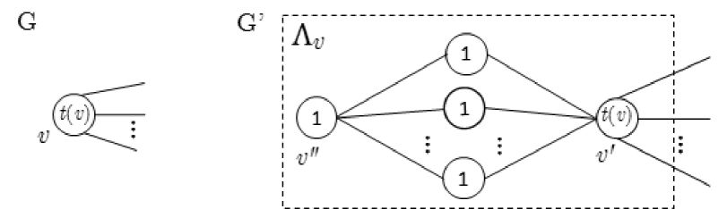
Figure 1: The gadget ${\Lambda}_{v}$: (left) a generic vertex $v\in V$ having degree $d_{G}(v)$ and threshold $t(v)$; (right) the gadget ${\Lambda}_{v}$, having $d_{G}(v)+2$ vertices, associated to $v$.

3 The Algorithm for Weighted Target Set Selection

Our algorithm WTSS works by iteratively deleting vertices from the input graph $G$. At each iteration, the vertex to be deleted is chosen as to maximize a certain function (Case 3). During the deletion process, some vertex $v$ in the surviving graph may remain with less neighbors than its threshold; in such a case (Case 2) $v$ is added to the target set and deleted from the graph while its neighbors’ thresholds are decreased by $1$ (since they receive $v$’s influence). It can also happen that the surviving graph contains a vertex $v$ whose threshold has been decreased down to $0$ (e.g., the deleted vertices are able to activate $v$); in such a case (Case 1) $v$ is deleted from the graph and its neighbors’ thresholds are decreased by $1$ (since as soon as vertex $v$ activates, its neighbors will receive $v$’s influence).

Input: A graph $G=(V,E)$ with thresholds $t(v)$ and costs $c(v)$, for $v\in V$.

Output: A target set $S$ for $G$.

1 $S=\emptyset$;

2 $U=V$;

3 foreach $v\in V$ do

4       ${\delta}(v)=d_{G}(v)$;

5       $k(v)=t(v)$;

6       $N(v)=\Gamma_{G}(v)$;

7while  $U\neq\emptyset$  do // Select one vertex and eliminate it from the graph.

8       if there exists $v\in U$ s.t. $k(v)=0$ then // Case 1: The vertex $v$ is activated by the influence of its neighbors in $V-U$ only; it can then influence its neighbors in $U$.

9             foreach $u\in N(v)$ do

10                   $k(u)=\max(k(u)-1,0)$;

11            

12      else

13             if  there exists $v\in U$ s.t. ${\delta}(v)<k(v)$ then // Case 2: $v$ is added to $S$, since not enough neighbors remain in $U$ to activate it; $v$ can then influence its neighbors in $U$.

14                  $S=S\cup\{v\}$;

15                   foreach $u\in N(v)$ do

16                         $k(u)=k(u)-1$;

17                  

18            else

19                   // Case 3: The vertex $v$ will be activated its neighbors in $U$.

20                   $v={\tt argmax}_{u\in U}\left\{\frac{c(u)\,k(u)}{\delta(u)(\delta(u)+1)}\right\}$;

21            

22      foreach $u\in N(v)$ do // Remove the selected vertex $v$ from the graph.

23             ${\delta}(u)={\delta}(u)-1$;

24             $N(u)=N(u)-\{v\}$;

25      $U=U-\{v\}$;

Algorithm 1    Algorithm WTSS($G$)

Example 2.

Consider the tree $T$ in Figure 2. The number inside each circle is the vertex threshold and $c(v)=t(v)$, for each $v$. The algorithm removes vertices from $T$ as in the table below where, for each iteration of the while loop, we give the selected vertex and which among Cases 1, 2 or 3 applies.

Iteration	1	2	3	4	5	6	7	8	9	10
Vertex	$v_{5}$	$v_{10}$	$v_{6}$	$v_{9}$	$v_{7}$	$v_{8}$	$v_{1}$	$v_{4}$	$v_{3}$	$v_{2}$
Case	3	3	2	3	3	2	3	2	2	2

The set returned by the algorithm is $S=\{v_{2},v_{3},v_{4},v_{6},v_{8}\}$, a target set having cost ${C}(S)=5$.

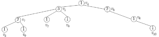
Figure 2: The tree of Example 2. The number inside each circle rewpresents the vertex threshold.

The algorithm WTSS is a generalization to weighted graphs of the TSS algorithm presented in [18]. The correctness of the algorithm WTSS does not depend on the cost values, hence it immediately follows from the correctness proof given in [18]. Moreover a proof on the bound on the target set size can be immediately obtained from the proof of the corresponding bound in [18]—by appropriately substituting the threshold value $t(v)$ by the weighted value $c(v)t(v)$ in the proof.

Theorem 2.

For any graph $G$ and threshold function $t$ the algorithm WTSS($G$) outputs a target set for $G$. The algorithm can be implemented so to run in time $O(|E|\log|V|)$. Moreover, the algorithm WTSS($G$) returns a target set $S$ of cost

$${C}(S)\leq\sum_{v\in V}\frac{c(v)t(v)}{d_{G}(v)+1}.$$ (1)

Theorem 3.

The algorithm WTSS($G$) outputs an optimal target set if $G$ is a complete graph such that $c(v)\leq c(u)$ whenever $t(v)\leq t(u)$.

Proof.   We denote by $v_{i}$ the vertex selected during the $n-i+1$-th iteration of the while loop in the algorithm WTSS and by ${{\cal G}}(i)$ the graph induced by the vertices $v_{i},\ldots,v_{1}$, for $i=n,\ldots,1$. We show that for each $i=1,\ldots,n$ it holds that $S\cap\{v_{i},\ldots,v_{1}\}$ is optimal for ${{\cal G}}(i)$. Consider first ${{\cal G}}(1)$ consisting of the isolated vertex $v_{1}$ with threshold $k_{1}(v_{1})$. It holds

$${C}(S\cap\{v_{1}\})=\begin{cases}{{C}(\emptyset)=0}&{if\ k_{1}(v_{1})=0}\\ {{C}(\{v_{1}\})=c(v_{1})}&{if\ k_{1}(v_{1})>0}\end{cases}$$

which is optimal. Suppose now ${C}(S\cap\{v_{i-1},\ldots,v_{1}\})$ is optimal for ${{\cal G}}(i-1)$ and consider ${{\cal G}}(i)$. The selected vertex is $v_{i}$.
If $k_{i}(v_{i})=0$ then it is obvious that no optimal solution for ${{\cal G}}(i)$ includes the “already” active vertex $v_{i}$. Hence, the inductive hypothesis on ${{\cal G}}(i-1)$ implies that ${C}(S\cap\{v_{i},\ldots,v_{1}\})={C}(S\cap\{v_{i-1},\ldots,v_{1}\})$ is optimal for ${{\cal G}}(i)$.
If $k_{i}(v_{i})>{\delta}_{i}(v_{i})=i-1$ then any optimal solution for ${{\cal G}}(i)$ includes vertex $v_{i}$ (which cannot be influenced otherwise) and the optimality follows by the optimality hypothesis on ${{\cal G}}(i-1)$.
If none of the above holds, then $0<k_{i}(v_{j})\leq{\delta}_{i}(v_{j})$, for each $j\leq i$, and $c(v_{i})k_{i}(v_{i})\geq c(v_{j})k_{i}(v_{j})$, for each $j\leq i-1$. We show now that there exists at least one optimal solution for ${{\cal G}}(i)$ which does not include $v_{i}$. Consider an optimal solution $S^{*}_{i}$ for ${{\cal G}}(i)$ and assume $v_{i}\in S^{*}_{i}$. Let

$$v=\operatorname*{arg\,max}_{\genfrac{}{}{0.0pt}{}{1\leq j\leq i-1}{v_{j}\notin S^{*}_{i}}}k_{i}(v_{j}).$$

By hypothesis the costs are ordered according to the initial thresholds of the vertices. Since at each step either all thresholds are decreased or they are all left equal, we have that $c(v_{j})k_{i}(v_{j})\leq c(v_{h})k_{i}(v_{h})$ whenever $c(v_{j})\leq c(v_{h})$. Hence, ${C}(S^{*}_{i}-\{v_{i}\}\cup\{v\})\leq{C}(S^{*}_{i})$. Moreover, recalling that $k_{i}(v_{i})\leq{\delta}_{i}(v_{i})$ we know that $S^{*}_{i}-\{v_{i}\}\cup\{v\}$ is a solution for ${{\cal G}}(i)$.
We have then found an optimal solution that does not contain $v_{i}$. This fact and the optimality hypothesis on ${{\cal G}}(i-1)$ imply the optimality of $S\cap\{v_{i},\ldots,v_{1}\}=S\cap\{v_{i-1},\ldots,v_{1}\}$. $\Box$

4 Targeting with Partial Incentives

In this section, we design an algorithm to efficiently allocate incentives to the vertices of a network, in such a way that it triggers an influence diffusion process that influences the whole network. The algorithm is called TPI($G$). It is close in spirit to the algorithm WTSS$(G)$, with some crucial differences. Again the algorithm proceeds by iteratively deleting vertices from the graph and at each iteration the vertex to be deleted is chosen as to maximize a certain parameter (Case 2). If, during the deletion process, a vertex $v$ in the surviving graph remains with less neighbors than its remaining threshold (Case 1), then $v$’s partial incentive is increased so that the $v$’s remaining threshold is at least as large as the number of $v$’s neighbors in the surviving graph.

Input: A graph $G=(V,E)$ with thresholds $t(v)$, for each $v\in V$.

Output: ${\bf s}$ a target vector for $G$.

1 $U=V$;

2 foreach $v\in V$ do

3       $s(v)=0;$ // Partial incentive initially assigned to $v$.

4       ${\delta}(v)=d_{G}(v)$;

5       $k(v)=t(v)$;

6       $N(v)=\Gamma_{G}(v)$;

7while  $U\neq\emptyset$  do // Select one vertex and either update its incentive or remove it from the graph.

8       if there exists $v\in U$ s.t. $k(v)>{\delta}(v)$ then // Case 1: Increase $s(v)$ and update $k(v)$.

9             $s(v)=s(v)+k(v)-{\delta}(v)$;

10             $k(v)={\delta}(v)$;

11             if k(v)=0 then // here  ${\delta}(v)=0$.

12                  $U=U-\{v\};$

13            

14      else // Case 2: Choose a vertex $v$ to eliminate from the graph.

15             $v={\tt argmax}_{u\in U}\left\{\frac{k(u)(k(u)+1)}{\delta(u)(\delta(u)+1)}\right\}$;

16             foreach $u\in N(v)$ do

17                   ${\delta}(u)={\delta}(u)-1$;

18                   $N(u)=N(u)-\{v\};$

19            $U=U-\{v\};$

20      

Algorithm 2    Algorithm TPI($G$)

Example 3.

Consider a complete graph on 7 vertices with thresholds $t(v_{1})=\ldots=t(v_{5})=1$, $t(v_{6})=t(v_{7})=6$ (cfr. Fig. 3). A possible execution of the algorithm is summarized below. At each iteration of the while loop, the algorithm considers the vertices in the order shown in the table below, where we also indicate for each vertex whether Cases 1 or 2 applies and the updated value of the partial incentive for the selected vertex:

Iteration	1	2	3	4	5	6	7	8
vertex	$v_{7}$	$v_{6}$	$v_{6}$	$v_{1}$	$v_{2}$	$v_{3}$	$v_{4}$	$v_{5}$
Case	2	1	2	2	2	2	2	1
Incentive	$0$	$1$	$1$	$0$	$0$	$0$	$0$	$1$

The algorithm $TPI(G)$ outputs the vector of partial incentives having non zero elements $s(v_{5})=s(v_{6})=1$, for which we have

$${{\sf Active}}[{\bf s},0] = \{v_{5}\}\qquad\mbox{\em(since $s(v_{5})=1=t(v_{5})$)}$$

$${{\sf Active}}[{\bf s},1] = {{\sf Active}}[{\bf s},0]\cup\{v_{1},v_{2},v_{3},v_{4}\}=\{v_{1},v_{2},v_{3},v_{4},v_{5}\}$$

$${{\sf Active}}[{\bf s},2] = {{\sf Active}}[{\bf s},1]\cup\{v_{6}\}=\{v_{1},v_{2},v_{3},v_{4},v_{5},v_{6}\}\qquad\mbox{\em(since $s(v_{6})=1$)}$$

$${{\sf Active}}[{\bf s},3] = {{\sf Active}}[{\bf s},2]\cup\{v_{7}\}=V.$$

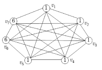
Figure 3: A complete graph example. The number inside each circle is the vertex threshold.

We first prove the algorithm correctness, next we give a general upper bound on the size $\sum_{v\in V}s(v)$ of its output and prove its optimality for trees and cliques.

To this aim we will use the following notation.

Let $\ell$ be the number of iterations of the while loop in TPI($G$). For each iteration $j$, with $1\leq j\leq\ell$, of the while loop we denote

• by $U_{j}$ the set $U$ at the beginning of the $j$-th iteration (cfr. line 7 of $TPI(G)$), in particular $U_{1}=V(G)$ and $U_{\ell+1}=\emptyset$;

• by ${{\cal G}}(j)$ the subgraph of $G$ induced by the vertices in $U_{j}$,

• by ${v_{j}}$ the vertex selected during the $j$-th iteration,

• by ${\delta}_{j}(v)$ the degree of vertex $v$ in ${{\cal G}}(j)$,

• by $k_{j}(v)$ the value of the remaining threshold of vertex $v$ in ${{\cal G}}(j)$, that is, as it is updated at the beginning of the $j$-th iteration, in particular $k_{1}(v)=t(v)$ for each $v\in V$,

• by $s_{j}(v)$ the partial incentive collected by vertex $v$ in ${{\cal G}}(j)$ starting from the $j$-th iteration, in particular we set $s_{\ell+1}(v)=0$ for each $v\in V$;

• by ${\sigma}_{j}$ the increment of the partial incentives during the $j$-th iteration, that is,

  $${\sigma}_{j}=s_{j}(v_{j})-s_{j+1}(v_{j})=\begin{cases}{0}&{\mbox{if}\ k_{j}({v_{j}})\leq{\delta}_{j}({v_{j}}),}\\ {k_{j}({v_{j}})-{\delta}_{j}({v_{j}})}&{\mbox{otherwise.}}\end{cases}$$

According to the above notation, we have that if vertex $v$ is selected during the iterations $j_{1}<j_{2}<\ldots<j_{a-1}<j_{a}$ of the while loop in TPI($G$), where the last value $j_{a}$ is the iteration when $v$ has been eliminated from the graph, then

$$s_{j}(v)=\begin{cases}{{\sigma}_{j_{1}}+{\sigma}_{j_{2}}+\ldots+{\sigma}_{j_{a}}}&{\mbox{if}\ j\leq j_{1},}\\ {{\sigma}_{j_{b}}+{\sigma}_{j_{b+1}}+\ldots+{\sigma}_{j_{a}}}&{\mbox{if}\ j_{b-1}<j\leq j_{b}{\leq j_{a}},}\\ {0}&{\mbox{if}\ j>j_{a}.}\end{cases}$$

In particular when $j=j_{a}$, it holds that $s_{j}(v)={\sigma}_{j}$.

The following result is immediate.

Proposition 1.

Consider the vertex ${v_{j}}$ that is selected during iteration $j$, for $1\leq j\leq\ell$, of the while loop in the algorithm TPI($G$):

• If Case 1 of the algorithm TPI($G$) holds and ${\delta}_{j}({v_{j}})=0$, then $k_{j}({v_{j}})>{\delta}_{j}({v_{j}})=0$ and the isolated vertex ${v_{j}}$ is eliminated from ${{\cal G}}(j)$. Moreover,
  

  $$U_{j+1}=U_{j}-\{{v_{j}}\},\quad s_{j+1}({v_{j}})=s_{j}({v_{j}})-{\sigma}_{j},\quad{\sigma}_{j}=k_{j}({v_{j}})-{\delta}_{j}({v_{j}})=k_{j}({v_{j}})>0,$$

  and, for each $v{\in}U_{j+1}$

  $$s_{j+1}(v)=s_{j}(v),\quad{\delta}_{j+1}(v)={\delta}_{j}(v),\quad k_{j+1}(v)=k_{j}(v).$$

• If Case 1 of TPI($G$) holds with ${\delta}_{j}({v_{j}})>0$, then $k_{j}({v_{j}})>{\delta}_{j}({v_{j}})>0$ and no vertex is deleted from ${{\cal G}}(j)$, that is, $U_{j+1}=U_{j}$. Moreover,

  $${\sigma}_{j}=k_{j}({v_{j}})-{\delta}_{j}({v_{j}})>0$$

  and, for each $v\in U_{j+1}$

  $${\delta}_{j+1}(v)={\delta}_{j}(v),\quad s_{j+1}(v)=\begin{cases}{s_{j}({v_{j}}){-}{\sigma}_{j}}&{\mbox{if }v={v_{j}}}\\ {s_{j}(v)}&{\mbox{if }v\neq{v_{j}}}\end{cases},\ \quad k_{j+1}(v)=\begin{cases}{{\delta}_{j}(v)}&{\mbox{if}\ v={v_{j}}}\\ {k_{j}(v)}&{\mbox{if}\ v\neq{v_{j}}}.\end{cases}$$

• If Case 2 of TPI($G$) holds then $k_{j}({v_{j}})\leq{\delta}_{j}({v_{j}})$ and ${v_{j}}$ is pruned from ${{\cal G}}(j)$. Hence,

  $$U_{j+1}=U_{j}-\{{v_{j}}\},\qquad{\sigma}_{j}=0,$$

  and, for each $v\in U_{j+1}$ it holds

  $$s_{j+1}(v)=s_{j}(v),\quad k_{j+1}(v)=k_{j}(v)\quad{\delta}_{j+1}(v)=\begin{cases}{{\delta}_{j}(v)-1}&{\mbox{if}\ v\in\Gamma_{{{\cal G}}(j)}({v_{j}})}\\ {{\delta}_{j}(v)}&{\mbox{otherwise.}}\end{cases}$$

Lemma 1.

For each iteration $j=1,2,\ldots,\ell$, of the while loop in the algorithm TPI($G$),

• if $\ k_{j}({v_{j}})>{\delta}_{j}({v_{j}})$ then ${\sigma}_{j}=k_{j}({v_{j}})-{\delta}_{j}({v_{j}})=1$;

• if ${\delta}_{j}({v_{j}})=0$ then $s_{j}({v_{j}})=k_{j}({v_{j}})$.

Proof.   First, we prove 1). At the beginning of the algorithm, $t(u)=k(u)\leq d(u)={\delta}(u)$ holds for all $u\in V$. Afterwords, the value of ${\delta}(u)$ is decreased by at most one unit for each iteration (cfr. line 16 of TPI($G$)). Moreover, the first time the condition of Case 1 holds for some vertex $u$, one has ${\delta}_{j}(u)=k_{j}(u)-1$. Hence, if the selected vertex is $v_{j}=u$ then 1) holds; otherwise, some $v_{j}\neq u$, satisfying the condition of Case 1 is selected and ${\delta}_{j+1}(u)={\delta}_{j}(u)$ and $k_{j+1}(u)=k_{j}(u)$ hold. Hence, when at some subsequent iteration $j^{\prime}>j$ the algorithm selects $v_{j^{\prime}}=u$, it holds ${\delta}_{j^{\prime}}(u)=k_{j^{\prime}}(u)-1$.
To show 2), it is sufficient to notice that at the iteration $j$ when vertex $v_{j}$ is eliminated from the graph, it holds $s_{j}(v)={\sigma}_{j}$.

$\Box$

Next theorem states the correctness of the algorithm TPI($G$) for any graph $G$.

Theorem 4.

For any graph $G$ the algorithm TPI($G$) outputs a target vector for $G$.

Proof.   We show that for each iteration $j$, with $1\leq j\leq\ell$, the assignation of partial incentives $s_{j}(v)$ for each $v\in U_{j}$ activates all the vertices of the graph ${{\cal G}}(j)$ when the distribution of thresholds to its vertices is $k_{j}(\cdot)$. The proof is by induction on $j$.
If $j=\ell$ then the unique vertex $v_{\ell}$ in ${{\cal G}}(\ell)$ has degree ${\delta}_{\ell}(v_{\ell})=0$ and $s_{\ell}(v_{\ell})=k_{\ell}(v_{\ell})=1$ (see Lemma 1).
Consider now $j<\ell$ and suppose the algorithm be correct on ${{\cal G}}(j+1)$ that is, the assignation of partial incentives $s_{j+1}(v)$, for each $v\in U_{j+1}$, activates all the vertices of the graph ${{\cal G}}({j+1})$ when the distribution of thresholds to its vertices is $k_{j+1}(\cdot)$.
Recall that $v_{j}$ denotes the vertex the algorithm selects from $U_{j}$ (thus obtaining $U_{j+1}$, the vertex set of ${{\cal G}}(j+1)$). In order to prove the theorem we analyze three cases according to the current degree and threshold of the selected vertex $v_{j}$.

• Let $k_{j}({v_{j}})>{\delta}_{j}({v_{j}})=0$. By Lemma 1, we have $k_{j}({v_{j}})=s_{j}({v_{j}})$. Furthermore, recalling that 1.1) of Proposition 1 holds and by using the inductive hypothesis on ${{\cal G}}(j+1)$, we get the correctness on ${{\cal G}}(j)$ .

• Let $k_{j}({v_{j}})>{\delta}_{j}({v_{j}})\geq 1$. By recalling that 1.2) of Proposition 1 holds we get $k_{j}(v)-s_{j}(v)=k_{j+1}(v)-s_{j+1}(v)$, for each vertex $v\in U_{j}$. Indeed, for each $v\neq v_{j}$ we have $k_{j+1}(v)=k_{j}(v)$ and $s_{j+1}(v)=s_{j}(v)$. Moreover,

  $$k_{j+1}({v_{j}})-s_{j+1}({v_{j}})={\delta}_{j}({v_{j}})-s_{j}({v_{j}})+{\sigma}_{j}=k_{j}({v_{j}})-s_{j}({v_{j}}).$$

  Hence the vertices that can be activated in ${{\cal G}}(j+1)$ can be activated in ${{\cal G}}(j)$ with thresholds $k_{j}(\cdot)$ and partial incentives $s_{j}(\cdot)$. So, by using the inductive hypothesis on ${{\cal G}}(j+1)$, we get the correctness on ${{\cal G}}(j)$.

• Let $k_{j}({v_{j}})\leq{\delta}_{j}({v_{j}})$. By recalling that 2) of Proposition 1 holds and by the inductive hypothesis on ${{\cal G}}(j+1)$ we have that all the neighbors of ${v_{j}}$ in ${{\cal G}}(j)$ that are vertices in $U_{j+1}$ gets active; since $k_{j}({v_{j}})\leq{\delta}_{j}({v_{j}})$ also ${v_{j}}$ activates in ${{\cal G}}(j)$.

$\Box$

We now give an upper bound on the size of the solution returned by the algorithm TPI.

Theorem 5.

For any graph $G$ the algorithm TPI($G$) returns a target vector ${\bf s}$ for $G$ such that

$$C({\bf s})=\sum_{v\in V}s(v)\leq\sum_{v\in V}\frac{t(v)(t(v)+1)}{2(d_{G}(v)+1)}$$

Proof.   Define ${\rm B}(j)=\sum_{v\in U_{j}}\frac{k_{j}(v)(k_{j}(v)+1)}{2({\delta}_{j}(v)+1)}$, for each $j=1,\ldots,\ell$. By definition of $\ell$, we have ${{\cal G}}(\ell+1)$ is the empty graph; we then define ${\rm B}(\ell+1)=0$. We prove now by induction on $j$ that

$${\sigma}_{j}\leq{\rm B}(j)-{\rm B}(j+1).$$ (2)

By using (2) we will have the bound on $\sum_{v\in V}s(v)$. Indeed,

$$\sum_{v\in V}s(v)=\sum_{j=1}^{\ell}{\sigma}_{j}\leq\sum_{j=1}^{\ell}({\rm B}(j)-{\rm B}(j+1))={\rm B}(1)-{\rm B}(\ell+1)={\rm B}(1)=\sum_{v\in V}\frac{t(v)(t(v)+1)}{2(d(v)+1)}.$$

In order to prove (2), we analyze three cases depending on the relation between $k_{j}({v_{j}})$ and ${\delta}_{j}({v_{j}})$.
$\bullet$ Assume first $k_{j}({v_{j}})>{\delta}_{j}({v_{j}})=0$. We get

$${\rm B}(j)-{\rm B}(j{+}1) = \sum_{v\in U_{j}}\frac{k_{j}(v)(k_{j}(v)+1)}{2(\delta_{j}(v)+1)}-\sum_{v\in U_{j+1}}\frac{k_{j+1}(v)(k_{j+1}(v)+1)}{2(\delta_{j+1}(v)+1)}$$

$$= \frac{k_{j}({v_{j}})(k_{j}({v_{j}})+1)}{2(\delta_{j}(v_{j})+1)}+\sum_{v\in U_{j}-\{v_{j}\}}\frac{k_{j}(v)(k_{j}(v)+1)}{2(\delta_{j}(v)+1)}$$

$$\hphantom{aaaaaaaaaaaaaaa}-\sum_{v\in U_{j+1}}\frac{k_{j+1}(v)(k_{j+1}(v)+1)}{2(\delta_{j+1}(v)+1)}$$

$$= \frac{k_{j}({v_{j}})(k_{j}({v_{j}})+1)}{2(\delta_{j}(v_{j})+1)}\qquad\qquad\mbox{{(by 1.1 in Proposition \ref{prop1})}}$$

$$= 1={\sigma}_{j}.\qquad\qquad\qquad\qquad\qquad\mbox{{(by Lemma \ref{d=0})}}$$

$\bullet$ Let now $k_{j}({v_{j}})>{\delta}_{j}({v_{j}})\geq 1$. We have

$${\rm B}(j)-{\rm B}(j{+}1) = \sum_{v\in U_{j}}\frac{k_{j}(v)(k_{j}(v)+1)}{2(\delta_{j}(v)+1)}-\sum_{v\in U_{j+1}}\frac{k_{j+1}(v)(k_{j+1}(v)+1)}{2(\delta_{j+1}(v)+1)}$$

$$= \frac{k_{j}({v_{j}})(k_{j}({v_{j}}){+}1)}{2(\delta_{j}(v_{j})+1)}-\frac{k_{j+1}({v_{j}})(k_{j+1}({v_{j}}){+}1)}{2(\delta_{j+1}(v_{j})+1)}$$

$$+\sum_{v\in U_{j}-\{v_{j}\}}\frac{k_{j}(v)(k_{j}(v)+1)}{2(\delta_{j}(v)+1)}-\sum_{v\in U_{j+1}-\{v_{j}\}}\frac{(k_{j+1}(v)(k_{j+1}(v)+1)}{2(\delta_{j+1}(v)+1)}$$

$$= \frac{(\delta_{j}(v_{j})+1)(\delta_{j}(v_{j})+2)}{2(\delta_{j}(v_{j})+1)}-\frac{\delta_{j}(v_{j})(\delta_{j}(v_{j})+1)}{2(\delta_{j}(v_{j})+1)}\ \ \mbox{{(by 1.2 in Proposition \ref{prop1})}}$$

$$= \frac{2(\delta_{j}(v_{j})+1)}{2(\delta_{j}(v_{j})+1)}=1={\sigma}_{j}.\qquad\qquad\qquad\qquad\qquad\mbox{{(by Lemma \ref{d=0})}}$$

$\bullet$ Finally, let $k_{j}({v_{j}})\leq{\delta}_{j}({v_{j}})$. In this case, by the algorithm we know that

$$\frac{k_{j}(v)(k_{j}(v)+1)}{\delta_{j}(v)(\delta_{j}(v)+1)}\leq\frac{k_{j}({v_{j}})(k_{j}({v_{j}})+1)}{\delta_{j}({v_{j}})(\delta_{j}({v_{j}})+1)},$$ (3)

for each $v\in U_{j}$. Hence, we get

$${\rm B}(j)-{\rm B}(j+1) = \sum_{v\in U_{j}}\frac{k_{j}(v)(k_{j}(v)+1)}{2(\delta_{j}(v)+1)}-\sum_{v\in U_{j+1}}\frac{k_{j+1}(v)(k_{j+1}(v)+1)}{2(\delta_{j+1}(v)+1)}$$

$$= \frac{k_{j}({v_{j}})(k_{j}({v_{j}}){+}1)}{2(\delta_{j}(v_{j}){+}1)}+\sum_{v\in\Gamma_{{{\cal G}}(j)}(v_{j})}\frac{k_{j}(v)(k_{j}(v){+}1)}{2(\delta_{j}(v){+}1)}$$

$$\hphantom{a}-\sum_{v\in\Gamma_{{{\cal G}}(j)}(v_{j})}\frac{k_{j+1}(v)(k_{j+1}(v){+}1)}{2(\delta_{j+1}(v){+}1)}\qquad\qquad\mbox{(by 2 in Proposition \ref{prop1})}$$

$$= \frac{k_{j}({v_{j}})(k_{j}({v_{j}}){+}1)}{2(\delta_{j}(v_{j}){+}1)}+\sum_{v\in\Gamma_{{{\cal G}}(j)}(v_{j})}\frac{k_{j}(v)(k_{j}(v){+}1)}{2}\left(\frac{1}{(\delta_{j}(v)+1)}-\frac{1}{\delta_{j}(v)}\right)$$

$$= \frac{k_{j}({v_{j}})(k_{j}({v_{j}})+1)}{2(\delta_{j}(v_{j})+1)}-\sum_{v\in\Gamma_{{{\cal G}}(j)}(v_{j})}\frac{k_{j}(v)(k_{j}(v)+1)}{2\delta_{j}(v)(\delta_{j}(v)+1)}$$

$$\geq \frac{k_{j}({v_{j}})(k_{j}({v_{j}})+1)}{2(\delta_{j}(v_{j})+1)}-\frac{k_{j}(v_{j})(k_{j}(v_{j})+1)\delta_{j}(v_{j})}{2\delta_{j}(v_{j})(\delta_{j}(v_{j})+1)}\ \ \qquad\mbox{(by (\ref{argmaxEq}))}$$

$$= 0={\sigma}_{j}\qquad\qquad\qquad\qquad\qquad\qquad\qquad\qquad\qquad\qquad\qquad\qquad\Box$$

4.1 Complete graphs

Theorem 6.

TPI($K$) returns an optimal target vector for any complete graph $K$.

Proof.   We will show that, for each $j=\ell,\cdots,1$, the incentives $s_{j}(v)$ for $v\in U_{j}$ are optimal for ${{\cal K}}(j)$ when the distribution of thresholds to its vertices is $k_{j}(\cdot)$. In particular, we will prove that

$${S}_{j}=\sum_{h\geq j}{\sigma}_{h}=\sum_{v\in U_{j}}s_{j}(v)=\sum_{v\in U_{j}}s^{*}_{j}(v)$$ (4)

for any optimal target vector ${\bf s}^{*}_{j}$ for ${{\cal K}}(j)$.

The theorem follows by setting $j=1$ (recall that ${{\cal K}}(1)=K$ and $s_{1}(v)=s(v)$, $k_{1}(v)=t(v)$ for each $v\in U_{1}=V(K)$). We proceed by induction on $j$.

For $j=\ell$, the graph ${{\cal K}}(\ell)$ consists of the unique vertex $v_{\ell}$ and by Lemma 1 and 1.1 of Proposition 1, it holds ${S}_{\ell}={\sigma}_{\ell}=s_{\ell}(v_{\ell})=k_{\ell}(v_{\ell})=1=s^{*}_{\ell}(v_{\ell})$.

Consider now some $j<\ell$ and suppose that the partial incentives $s_{j+1}(v)$ for $v\in U_{j+1}$ are optimal for ${{\cal K}}({j+1})$ when the distribution of thresholds is $k_{j+1}(\cdot)$. Consider the $j$-th iteration of the while loop in TPI($K$). First, notice that the complete graph ${{\cal K}}(j)$ cannot have isolated vertices; hence, only 1.2) and 2) in Proposition 1 can hold for the selected vertex ${v_{j}}$. We will prove that (4) holds. We distinguish two cases according to the value of the threshold $k_{j}({v_{j}})$.

Assume first that $k_{j}({v_{j}})>{\delta}_{j}({v_{j}})$. By 1.2) in Proposition 1 and the inductive hypothesis, we have

$${S}_{j}=\sum_{h\geq j}{\sigma}_{h}={\sigma}_{j}+\sum_{h\geq j+1}{\sigma}_{h}=k_{j}({v_{j}})-{\delta}_{j}({v_{j}})+\sum_{v\in U_{j+1}}s^{*}_{j+1}(v)\leq\sum_{v\in U_{j}}s^{*}_{j}(v)$$

where the inequality holds since any solution that optimally assigns incentives ${\bf s}^{*}_{j}$ to the vertices of ${{\cal K}}(j)$ increases by at least $k_{j}({v_{j}})-{\delta}_{j}({v_{j}})$ the sum of the optimal partial incentives assigned to the vertices in ${{\cal K}}(j+1)$.

Suppose now that $k_{j}({v_{j}})\leq{\delta}_{j}({v_{j}})$. By 2) in Proposition 1 and the inductive hypothesis we have

$$S_{j}=\sum_{h\geq j}{\sigma}_{h}={\sigma}_{j}+\sum_{h\geq j+1}{\sigma}_{h}=0+\sum_{v\in U_{j+1}}s^{*}_{j+1}(v).$$ (5)

We will show that, given any optimal incentive assignation $s^{*}_{j}(\cdot)$ to the vertices in ${{\cal K}}(j)$, it holds

$${S}_{j}\leq\sum_{v\in U_{j}}s^{*}_{j}(v).$$ (6)

thus proving (4) in this case. Consider the activation process in ${{\cal K}}(j)$ that starts with the partial incentives $s^{*}_{j}(\cdot)$ and let $\tau$ be the round during which vertex ${v_{j}}$ is activated, that is

$$\left|{{\sf Active}}[{\bf s}^{*}_{j},\tau-1]\cap\Gamma_{{{\cal K}}(j)}({v_{j}})\right|=k_{j}({v_{j}})-s^{*}_{j}({v_{j}}).$$ (7)

Equality (7) implies that there exist

$${\delta}_{j}({v_{j}})-(k_{j}({v_{j}})-s^{*}_{j}({v_{j}}))\geq{\delta}_{j}({v_{j}})-{\delta}_{j}({v_{j}})+s^{*}_{j}({v_{j}})=s^{*}_{j}({v_{j}})$$

neighbors of ${v_{j}}$ in ${{\cal K}}(j)$ that will be activated in some round larger or equal to $\tau$. Let $X$ be any subset of $s^{*}_{j}({v_{j}})$ such neighbors (i.,e., $|X|=s^{*}_{j}({v_{j}})$) and define

$$z_{j}(v)=\begin{cases}{s^{*}_{j}(v)+1}&{\mbox{if}\ v\in X,}\\ {s^{*}_{j}(v)}&{\mbox{if}\ v\in U_{j+1}-{X},}\\ {0}&{\mbox{if}\ v={v_{j}}.}\end{cases}$$ (8)

It is easy to see that the incentives $z_{j}(v)$ for $v\in U_{j}$ give a solution for ${{\cal K}}(j)$. Indeed, each vertex $v\in U_{j+1}-X$ activates at the same round as in the activation process starting with incentives $s^{*}_{j}$; furthermore, each vertex $v\in X$ can activate without the activation of ${v_{j}}$; finally, ${v_{j}}$ activates after both vertices in $U_{j+1}-X$ and vertices in $X$ are activated.
By the above and recalling 2) of Proposition 1, we have that $z_{j}(v)$ for $v\in U_{j+1}$ is a solution for ${{\cal K}}(j+1)$. Hence, $\sum_{v\in U_{j+1}}z_{j}(v)\geq\sum_{v\in U_{j+1}}s^{*}_{j+1}(v)$ and by (8) and (5) we have

$$\sum_{v\in U_{j}}s^{*}_{j}(v)=|X|+\sum_{v\in U_{j+1}}s^{*}_{j}(v)=\sum_{v\in U_{j+1}}z_{j}(v)\geq\sum_{v\in U_{j+1}}s^{*}_{j+1}(v)=S_{j}$$

thus proving (6). $\Box$

4.2 Trees

In this section we prove the optimality of the algorithm TPI when the input graph is a tree.

Theorem 7.

TPI($T$) outputs an optimal target vector for any tree $T$.

Proof.   We will show, for each $j=\ell,\cdots,1$, that the incentives $s_{j}(v)$ for $v\in U_{j}$ are optimal for the forest ${{\cal T}}(j)$ with thresholds $k_{j}(\cdot)$. In particular, we will prove that

$${S}_{j}=\sum_{h\geq j}{\sigma}_{h}=\sum_{v\in U_{j}}s_{j}(v)=\sum_{v\in U_{j}}s^{*}_{j}(v)$$ (9)

for any optimal target vector ${\bf s}^{*}_{j}$ for the vertices in $U_{j}=V({{\cal T}}(j))$.

The theorem will follow for $j=1$ (recall that ${{\cal T}}(1)=T$ and $s_{1}(v)=s(v)$, $k_{1}(v)=t(v)$ for each $v\in U_{1}=V(T)$). We proceed by induction on $j$.

For $j=\ell$, the graph ${{\cal T}}(\ell)$ consists of the unique vertex $v_{\ell}$ and by Lemma 1 and 1.1) in Proposition 1, it holds ${S}_{\ell}={\sigma}_{\ell}=s_{\ell}(v_{\ell})=k_{\ell}(v_{\ell})=1=s^{*}_{\ell}(v_{\ell})$.

Suppose now the partial incentives $s_{j+1}(v)$ for $v\in U_{j+1}$ are optimal for the forest ${{\cal T}}({j+1})$ when the thresholds are $k_{j+1}(\cdot)$, for some $j<\ell$.

Consider the $j$-th iteration of the while loop in TPI($T$). We will prove that (9) holds. We distinguish three cases according to the value of the $k_{j}({v_{j}})$ and ${\delta}_{j}({v_{j}})$.

Let $k_{j}({v_{j}})>{\delta}_{j}({v_{j}})=0$. In such a case $v_{j}$ is an isolated vertex. By Lemma 1, 1.1) of Proposition 1, and the inductive hypothesis we have

$${S}_{j}=\sum_{h\geq j}{\sigma}_{h}={\sigma}_{j}+\sum_{h\geq j+1}{\sigma}_{h}=k_{j}({v_{j}})+\sum_{v\in U_{j+1}}s^{*}_{j+1}(v)=1+\sum_{v\in U_{j+1}}s^{*}_{j+1}(v)\leq\sum_{v\in U_{j}}s^{*}_{j}(v).$$

Let $k_{j}({v_{j}})>{\delta}_{j}({v_{j}})>0$. By 1.2) in Proposition 1 and the inductive hypothesis we have

$${S}_{j}=\sum_{h\geq j}{\sigma}_{h}={\sigma}_{j}+\sum_{h\geq j+1}{\sigma}_{h}=k_{j}({v_{j}})-{\delta}_{j}({v_{j}})+\sum_{v\in U_{j+1}}s^{*}_{j+1}(v)\leq\sum_{v\in U_{j}}s^{*}_{j}(v),$$

where the inequality follows since any solution that optimally assigns partial incentives ${\bf s}^{*}_{j}$ to the vertices in ${{\cal T}}(j)$ increases of at least $k_{j}({v_{j}})-{\delta}_{j}({v_{j}})$ the sum of the optimal incentives assigned to the vertices in ${{\cal T}}(j+1)$.

Let $k_{j}({v_{j}})\leq{\delta}_{j}({v_{j}})$. By 2) in Proposition 1 and the inductive hypothesis we have

$$S_{j}=\sum_{h\geq j}{\sigma}_{h}={\sigma}_{j}+\sum_{h\geq j+1}{\sigma}_{h}=0+\sum_{v\in U_{j+1}}s^{*}_{j+1}(v)$$

In order to complete the proof in this case we will show that, given any optimal partial incentive assignment $s^{*}_{j}(\cdot)$ to the vertices in ${{\cal T}}(j)$, there is a cost equivalent optimal partial incentive assignment $z_{j}(\cdot)$ where $z_{j}(v_{j})=0$. Moreover, this solution activates also all the vertices in ${{\cal T}}(j+1)$. Hence

$${S}_{j}=\sum_{v\in U_{j}}s^{*}_{j}(v).$$ (10)

thus proving (9) in this case.
First of all we show that $k_{j}({v_{j}})={\delta}_{j}({v_{j}})$. Indeed, for each leaf $u\in U_{j}$ we have $k_{j}(u)={\delta}_{j}(u)=1$, which maximizes the value $\frac{k_{j}(u)(k_{j}(u)+1)}{{\delta}_{j}(u)({\delta}_{j}(u)+1)}$ since for any other vertex $v\in U_{j}$, $k_{j}(v)\leq{\delta}_{j}(v)$. Hence, $v_{j}$ is either a leaf vertex or an internal vertex with $k_{j}({v_{j}})={\delta}_{j}({v_{j}})$.
Let $\Gamma_{j}(v_{j})=\{u_{1},u_{2},\ldots,u_{{\delta}_{j}({v_{j}})}\}$ be the set of $v_{j}$’s neighbors. We have two cases to consider according to the value of $s^{*}_{j}(v_{j})$

• if $s^{*}_{j}(v_{j})=0$, then we have $s^{*}_{j}(\cdot)=z_{j}(\cdot)$. Since $k_{j}({v_{j}})={\delta}_{j}({v_{j}})$ and $s^{*}_{j}(v_{j})=0$, each vertex in $\Gamma_{j}(v_{j})$ is activated without the influence of $v_{j}$. Therefore, $s^{*}_{j}(\cdot)$ is also a solution for ${{\cal T}}(j+1)$.

• if $s^{*}_{j}(v_{j})>0$, then we can partition $\Gamma_{j}(v_{j})$ into two sets: $\Gamma^{\prime}_{j}(v_{j})$ and $\Gamma^{\prime\prime}_{j}(v_{j})$:

  • $\Gamma^{\prime}_{j}(v_{j})$ includes ${\delta}_{j}({v_{j}})-s^{*}_{j}(v_{j})$ vertices that are activated before $v_{j}$ (this set must exist otherwise $v_{j}$ will never activate);

  • $\Gamma^{\prime\prime}_{j}(v_{j})\subseteq\Gamma_{j}(v_{j})$ which consists of the remaining $s^{*}_{j}(v_{j})$ vertices.

  We define $z_{j}(\cdot)$ as follows:

  $$z_{j}(v)=\begin{cases}0&\mbox{ if }v=v_{j};\\ s^{*}_{j}(v)+1&\mbox{ if }v\in\Gamma^{\prime\prime}_{j}(v_{j});\\ s^{*}_{j}(v)&\mbox{ otherwise.}\end{cases}$$

  By construction we have that $\sum_{v\in U_{j}}z_{j}(v)=\sum_{v\in U_{j}}s^{*}_{j}(v)$. Moreover $z_{j}(v)$ activates all the vertices in ${{\cal T}}(j)$. In particular, the vertices in $\Gamma^{\prime}_{j}(v_{j})$ activate before $v_{j}$, while the vertices in $\Gamma^{\prime\prime}_{j}(v_{j})$ activate independently of $v_{j}$ thanks to the increased incentive. Therefore $v_{j}$ activates thanks to the vertices in $\Gamma_{j}(v_{j})$. A similar reasoning shows that $z_{j}(v)$ activates all the vertices in ${{\cal T}}(j+1)$.

$\Box$

We can also explicitly evaluate the cost of an optimal solution for any tree.

Theorem 8.

Any optimal target vector ${\bf s}^{*}$ on a tree $T$ with thresholds $t:V\longrightarrow{\mathbb{N}}$ has cost

$${C}({\bf s}^{*})=\sum_{v\in V}s^{*}(v)=|V|-1-\sum_{v\in V}d(v)-t(v).$$ (11)

Proof.   We proceed by structural induction on $T$. If $T$ consists of a single vertex $r$, then the optimal solution clearly has $s^{*}(r)=t(r)$. Hence, ${C}({\bf s}^{*})=s^{*}(r)=t(r)$ and 11) holds.
Let now $T$ be a tree, with at least two vertices, rooted in $r$. Let ${\bf s}^{*}$ be an optimal target vector for $T$. The optimality of ${\bf s}^{*}$ clearly implies that $s^{*}(r)\leq t(r)$. Therefore, the root $r$ needs to be influenced by $t(r)-s^{*}(r)\geq 0$ of its children. Once $r$ is activated, it can influence the remaining children. Summarizing, we have that there exists an ordering $v_{1},v_{2},\ldots,v_{d(r)}$ of $r$’s children such that,

$${C}({\bf s}^{*})=s^{*}(r)+\sum_{i=1}^{d(r)}{C}({\bf s}^{*}_{i}),$$ (12)

where ${\bf s}^{*}_{i}$ is an optimal target vector for the subtree $T(v_{i})$ rooted at $v_{i},$ assuming that each vertex $v$ in $T(v_{i})$ has threshold $t_{i}(v)$ given by

$$t_{i}(v)=\begin{cases}t(v)&\mbox{if ($v\neq v_{i}$ for $i=1,\ldots,d(r)$) or}\mbox{ ($v=v_{i}$ for some $1\leq i\leq t(r)-s^{*}(r)$)}\\ t(v_{i})-1&\mbox{if $v=v_{i}$ for some $t(r)-s^{*}(r)+1\leq i\leq d(r)$}.\end{cases}$$

Let $V_{i}$ denote the vertex set of $T(v_{i})$ and $d_{i}(v)$ denote the degree of $v$ in $T(v_{i})$—trivially, $d_{i}(v_{i})=d(v_{i})-1$ and $d_{i}(v)=d(v)$ for each $v\neq v_{i}$.

Assuming by induction that (11) holds for $T(v_{i})$, for $i=1,\ldots,d(r)$, by (12) we have

$${C}({\bf s}^{*}) = {\bf s}^{*}(r)+\sum_{i=1}^{d(r)}\left(|V_{i}|-1-\sum_{v\in V_{i}}d_{i}(v){-}t_{i}(v)\right)$$

$$= s^{*}(r)+\sum_{i=1}^{t(r)-s^{*}(r)}\left(|V_{i}|-1-\sum_{v\in V_{i}\atop v\neq v_{i}}(d(v){-}t(v))\ -\ (d(v_{i})-1)+t(v_{i})\right)$$

$$\qquad\ +\sum_{i=t(r)-s^{*}(r)+1}^{d(r)}\left(|V_{i}|-1-\sum_{v\in V_{i}\atop v\neq v_{i}}(d(v){-}t(v))\ -(d(v_{i})-1)+(t(v_{i})-1)\right)$$

$$= s^{*}(r)+\sum_{i=1}^{t(r)-s^{*}(r)}\left(|V_{i}|-\sum_{v\in V_{i}\atop}(d(v){-}t(v))\right)+\sum_{i=t(r)-s^{*}(r)+1}^{d(r)}\left(|V_{i}|-\sum_{v\in V_{i}}(d(v){-}t(v))-1\right)$$

$$= s^{*}(r)+\sum_{i=1}^{d(r)}|V_{i}|-\sum_{i=1}^{d(r)}\sum_{v\in V_{i}}(d(v){-}t(v))-(d(r)-t(r)+s^{*}(r))$$

$$= \left(|V|-1\right)-\sum_{v\in V}d(v){-}t(v)\qquad\qquad\qquad\qquad\qquad\qquad\qquad\qquad\qquad\qquad\qquad\quad\Box$$

5 Experiments

We have experimentally evaluated both our algorithms WTSS($G$) and TPI($G$) on real-world data sets and found that they perform quite satisfactorily. We conducted experiments on several real networks of various sizes from the Stanford Large Network Data set Collection (SNAP) [29], the Social Computing Data Repository at Arizona State University [38] and Newman’s Network data [33]. The data sets we considered include both networks for which “low cost” target sets exist and networks needing an expensive target sets (due to a community structure that appears to block the diffusion process).

5.1 Test settings

The competing algorithms. We compare the performance of our algorithms toward that of the best, to our knowledge, computationally feasible algorithms in the literature [19]. It is worth mentioning that the following competing algorithms were initially designed for the Maximally Influencing Set problem, where the goal is to identify a set $S\subseteq V$ such that its cost is bounded by a certain budget $\beta$ and the activation process activates as much vertices as possible. In order to compare such algorithms toward our strategies, for each algorithm we performed a binary search in order to find the smallest value of $\beta$ which allow to activate all the vertices of the considered graph. We compare the WTSS algorithm toward the following two algorithms:

• DegreeInt, a simple greedy algorithm, which selects vertices in descending order of degree [27, 9];

• DiscountInt, a variant of DegreeInt, which selects a vertex $v$ with the highest degree at each step. Then the degree of vertices in $\Gamma(v)$ is decreased by $1$ [9].

Moreover, we compare the TPI algorithm toward the following two algorithms:

• DegreeFrac, which selects each vertex fractionally proportional to its degree. Specifically, given a graph $G=(V,E)$ and budget $\beta$ this algorithm spend on each vertex $v\in V,$ $s(v)=\left\lfloor\frac{d(v)\times\beta}{2|E|}\right\rfloor$[19]. Remaining budget, if any, is assigned increasing by $1$ the budget assigned to some vertices (in descending order of degree).

• DiscountFrac, which at each step, selects the vertex $v$ having the highest degree and assigns to it a budged $s(v)=max(0,t(v)-|\Gamma(v)\cap S|))$, which represent the minimum amount that allows to activate $v$ ($S$ denotes the set of already selected vertices). As for the DiscountInt algorithm, after selecting a vertex $v$, the degree of vertices in $\Gamma(v)$ is decreased by $1$ [19].

Test Networks. The main characteristics of the studied networks are shown in Table 1. In particular, for each network we report the number of vertices, the number of edges, the maximum degree, the diameter, the size of the largest connected component, the number of triangles, the clustering coefficient and the network modularity.

Name	# of vert.	# of edges	Max deg	Diam.	Size of the LCC	Triangles	Clust Coeff	Modul.
Amazon0302 [29]	262111	1234877	420	32	262111	717719	0.4198	0.6697
BlogCatalog [38]	88784	4186390	9444	–	88784	51193389	0.4578	0.3182
BlogCatalog2 [38]	97884	2043701	27849	5	97884	40662527	0.6857	0.3282
BlogCatalog3 [38]	10312	333983	3992	5	10312	5608664	0.4756	0.2374
BuzzNet [38]	101168	4284534	64289	–	101163	30919848	0.2508	0.3161
ca-AstroPh [29]	18772	198110	504	14	17903	1351441	0.6768	0.3072
ca-CondMath [29]	23133	93497	279	14	21363	173361	0.7058	0.5809
ca-GrQc [29]	5242	14496	81	17	4158	48260	0.6865	0.7433
ca-HepPh [29]	10008	118521	491	13	11204	3358499	0.6115	0.5085
ca-HepTh [29]	9877	25998	65	17	8638	28399	0.5994	0.6128
Douban [38]	154907	327162	287	9	154908	40612	0.048	0.5773
Facebook [29]	4039	88234	1045	8	4039	1612010	0.6055	0.8093
Flikr [38]	80513	5899822	5706	–	80513	271601126	0.1652	–
Hep [29]	27770	352807	64	13	24700	1478735	0.3120	0.7203
Last.fm [38]	1191812	5115300	5140	–	1191805	3946212	0.1378	–
Livemocha [38]	104438	2196188	2980	6	104103	336651	0.0582	0.36
Power grid [33]	4941	6594	19	46	4941	651	0.1065	0.9306
Youtube2 [38]	1138499	2990443	28754	–	1134890	3056537	0.1723	0.6506

Table 1: Networks parameters.

Thresholds values. We tested with three categories of threshold function:

• Random thresholds where $t(v)$ is chosen uniformly at random in the interval $[1,d(v)]$;

• Constant thresholds where the thresholds are constant among all vertices (precisely the constant value is an integer in the interval $[2,10]$ and for each vertex $v$ the threshold $t(v)$ is set as $\min(t,d(v))$ where $t=2,3,\ldots,10$ (nine tests overall);

• Proportional thresholds where for each $v$ the threshold $t(v)$ is set as $\alpha\times d(v)$ with $\alpha=0.1,0.2,\ldots,0.9$ (nine tests overall). Notice that for $\alpha=0.5$ we are considering a particular version of the activation process named “majority” [22].

Costs. We report experiments results for the WTSS problem in case the costs are equal to the thresholds, that is $c(v)=t(v)$ for each vertex $v\in V$. Similar results hold for different cost choices.

	Targeting with Partial Incentives				Weighted Target Set Selection with $c(\cdot)=t(\cdot)$
Name	PTI	DiscountFrac	DegreeFrac		WTSS	DiscountInt	DegreeInt
Amazon0302	52703	328519 (623%)	879624 (1669%)		85410	596299 (698%)	890347 (1042%)
BlogCatalog	21761	824063 (3787%)	980670 (4507%)		82502	1799719 (2181%)	2066014 (2504%)
BlogCatalog2	16979	703383 (4143%)	178447 (1051%)		67066	1095580 (1634%)	1214818 (1811%)
BlogCatalog3	161	3890 (2416%)	3113 (1934%)		3925	3890 (99%)	3890 (99%)
BuzzNet	50913	1154952 (2268%)	371355 (729%)		166085	1838430 (1107%)	2580176 (1554%)
ca-AstroPh	4520	67189 (1486%)	198195 (4385%)		13242	183121 (1383%)	198195 (1497%)
ca-CondMath	5694	31968 (561%)	94288 (1656%)		10596	76501 (722%)	94126 (888%)
ca-GrQc	1422	5076 (357%)	15019 (1056%)		2141	12538 (586%)	15019 (701%)
ca-HepPh	4166	42029 (1009%)	120324 (2888%)		11338	118767 (1048%)	120324 (1061%)
ca-HepTh	2156	9214 (427%)	26781 (1242%)		3473	25417 (732%)	26781 (771%)
Douban	51167	140676 (275%)	345036 (674%)		91342	194186 (213%)	252739 (277%)
Facebook	1658	29605 (1786%)	54508 (3288%)		5531	77312 (1398%)	86925 (1572%)
Flikr	31392	2057877 (6555%)	134017 (427%)		110227	5359377 (4862%)	5879532 (5334%)
Hep	4122	11770 (286%)	33373 (810%)		5526	33211 (601%)	33373 (604%)
LastFM	296083	1965839 (664%)	4267035 (1441%)		631681	2681610 (425%)	4050280 (641%)
Livemocha	26610	861053 (3236%)	459777 (1728%)		57293	1799468 (3141%)	2189760 (3822%)
Power grid	767	2591 (338%)	4969 (648%)		974	3433 (352%)	4350 (447%)
Youtube2	313786	1210830 (386%)	3298376 (1051%)		576482	2159948 (375%)	3285525 (570%)

Table 2: Random Threshold Results.

5.2 Results

We compare the cost of the target set (or target vector) generated by six algorithms (PTI, DiscountFrac, DegreeFrac, WTSS, DiscountInt, DegreeInt) on $18$ networks, fixing the thresholds in $19$ different ways (Random, Constant with $t=2,3,\ldots,10$ and Proportional with $\alpha=0.1,0.2,\ldots,0.9$). Overall we performed $6\times 18\times 19=2052$ tests.

Random Thresholds.

Table 2 gives the results of the Random threshold test setting. Each number represents the cost of the target vector (left side of the table) or the target set (right side of the table) generated by each algorithm on each network using random thresholds (the same thresholds values have been used for all the algorithms). The value in bracket represents the overhead percentage compared to our algorithms (TPI for DiscountFrac and DegreeFrac and WTSS for DiscountInt and DegreeInt). Analyzing the results Table 2, we notice that in all the considered cases, with the exception of the network BlogCatolog3, our algorithms always outperform their competitors. In the network BlogCatalog3, the WTSS algorithm is slightly worse than its competitors but PTI performs much better than the other algorithms.

Constant and Proportional thresholds. The following figures depict the results of Constant and Proportional thresholds settings. For each network the results are reported in two separated figures: Proportional thresholds (left-side), the value of the $\alpha$ parameter appears along the $X$-axis, while the cost of the solution appears along the $Y$-axis; Constant thresholds (right-side), in this case the $X$-axis indicates the value of the thresholds. We present the results only for eight networks; the experiments performed on the other networks exhibit similar behaviors. Analyzing the results from Figures 4-6, we can make the following observations: In all the considered case our algorithms always outperform their competitors; the only algorithm that provides performance close to our algorithms is the DiscountFrac algorithm. However, for intermediate values of the $\alpha$ parameter, the gap to our advantage is quite significant. In general, in case of partial incentives we have even better results, the gap to our advantage increases with the increase of the parameter $\alpha$.

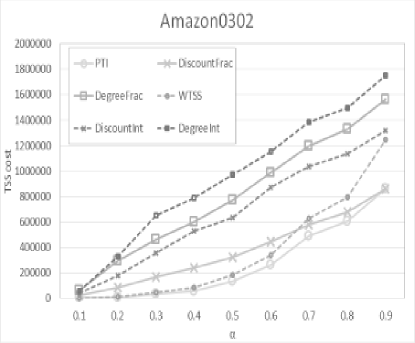
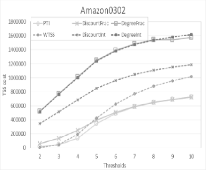
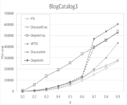
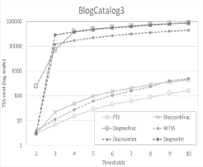
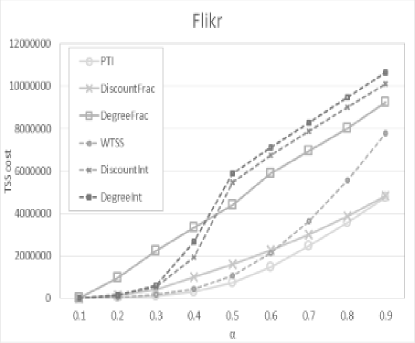
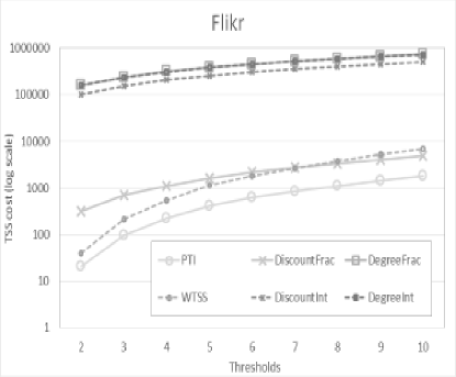
Figure 4: Amazon0302, BlogCatalog3, and Flikr results.

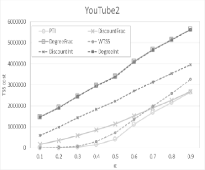
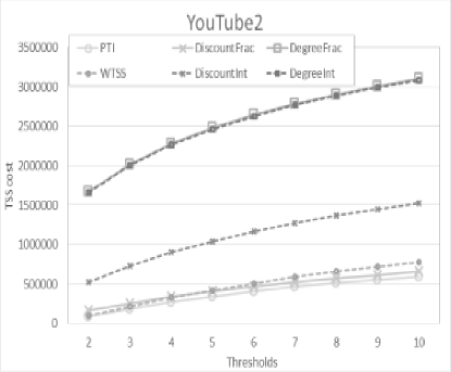
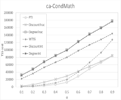
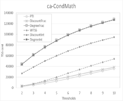
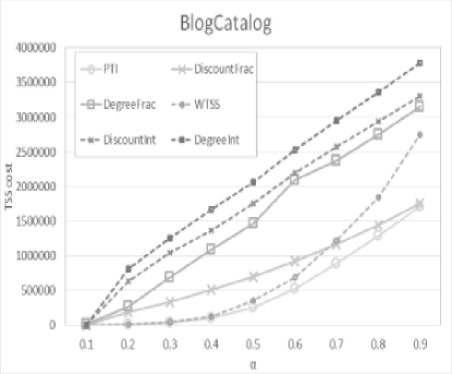
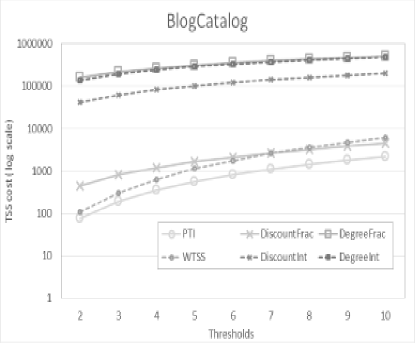
Figure 5: Youtube2, ca-CondMath, and BlogCatalog results.

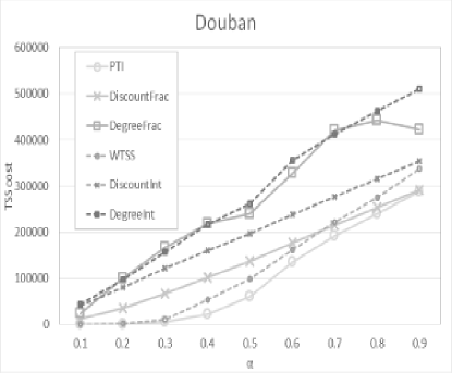
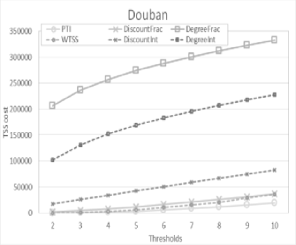
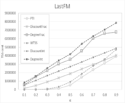
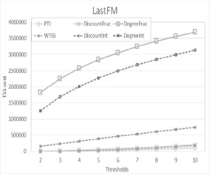
Figure 6: Douban and LastFM results.

References

- [1] Eyal Ackerman, Oren Ben-Zwi, and Guy Wolfovitz. Combinatorial model and bounds for target set selection. Theoretical Computer Science, 411(44 46):4017 – 4022, 2010.
- [2] Eytan Bakshy, Jake M. Hofman, Winter A. Mason, and Duncan J. Watts. Everyone’s an influencer: Quantifying influence on twitter. In Proceedings of the Fourth ACM International Conference on Web Search and Data Mining, WSDM ’11, pages 65–74, New York, NY, USA, 2011.
- [3] Cristina Bazgan, Morgan Chopin, André Nichterlein, and Florian Sikora. Parameterized approximability of maximizing the spread of influence in networks. Journal of Discrete Algorithms, 27:54 – 65, 2014.
- [4] Oren Ben-Zwi, Danny Hermelin, Daniel Lokshtanov, and Ilan Newman. Treewidth governs the complexity of target set selection. Discrete Optimization, 8(1):87 – 96, 2011.
- [5] Carmen C. Centeno, Mitre C. Dourado, Lucia Draque Penso, Dieter Rautenbach, and Jayme L. Szwarcfiter. Irreversible conversion of graphs. Theoretical Computer Science, 412(29):3693 – 3700, 2011.
- [6] Ching-Lueh Chang. Triggering cascades on undirected connected graphs. Information Processing Letters, 111(19):973 – 978, 2011.
- [7] Ning Chen. On the approximability of influence in social networks. SIAM Journal on Discrete Mathematics, 23(3):1400–1415, 2009.
- [8] W. Chen, C. Castillo, and L. Lakshmanan. Information and Influence Propagation in Social Networks. Morgan & Claypool, 2013.
- [9] Wei Chen, Yajun Wang, and Siyu Yang. Efficient influence maximization in social networks. In Proceedings of the 15th ACM SIGKDD International Conference on Knowledge Discovery and Data Mining, KDD ’09, pages 199–208, New York, NY, USA, 2009.
- [10] Chun-Ying Chiang, Liang-Hao Huang, Bo-Jr Li, Jiaojiao Wu, and Hong-Gwa Yeh. Some results on the target set selection problem. Journal of Combinatorial Optimization, 25(4):702–715, 2013.
- [11] Chun-Ying Chiang, Liang-Hao Huang, and Hong-Gwa Yeh. Target set selection problem for honeycomb networks. SIAM Journal on Discrete Mathematics, 27(1):310–328, 2013.
- [12] Morgan Chopin, André Nichterlein, Rolf Niedermeier, and Mathias Weller. Constant thresholds can make target set selection tractable. Theory of Computing Systems, 55(1):61–83, 2014.
- [13] Nicholas A. Christakis and James H. Fowler. The Collective Dynamics of Smoking in a Large Social Network. N Engl J Med, 358(21):2249–2258, May 2008.
- [14] Nicholas A. Christakis and James H. Fowler. Connected: The Surprising Power of Our Social Networks and How They Shape Our Lives – How Your Friends’ Friends’ Friends Affect Everything You Feel, Think, and Do. Back Bay Books, reprint edition, January 2011.
- [15] Ferdinando Cicalese, Gennaro Cordasco, Luisa Gargano, Martin Milanič, Joseph Peters, and Ugo Vaccaro. Spread of influence in weighted networks under time and budget constraints. Theoretical Computer Science, 586:40 – 58, 2015.
- [16] Ferdinando Cicalese, Gennaro Cordasco, Luisa Gargano, Martin Milanič, and Ugo Vaccaro. Latency-bounded target set selection in social networks. Theoretical Computer Science, 535:1 – 15, 2014.
- [17] Amin Coja-Oghlan, Uriel Feige, Michael Krivelevich, and Daniel Reichman. Contagious sets in expanders. In Proceedings of the Twenty-Sixth Annual ACM-SIAM Symposium on Discrete Algorithms, pages 1953–1987, 2015.
- [18] Gennaro Cordasco, Luisa Gargano, Marco Mecchia, Adele Anna Rescigno, and Ugo Vaccaro. A Fast and Effective Heuristic for Discovering Small Target Sets in Social Networks. In Proc. of 9th Annual International Conference on Combinatorial Optimization and Applications (COCOA 2015), volume LNCS 9486, pages 193–208, 2015.
- [19] Erik D. Demaine, Mohammad Taghi Hajiaghayi, Hamid Mahini, David L. Malec, S. Raghavan, Anshul Sawant, and Morteza Zadimoghadam. How to influence people with partial incentives. In Proceedings of the 23rd International Conference on World Wide Web, WWW ’14, pages 937–948, New York, NY, USA, 2014.
- [20] Pedro Domingos and Matt Richardson. Mining the network value of customers. In Proceedings of the Seventh ACM SIGKDD International Conference on Knowledge Discovery and Data Mining, KDD ’01, pages 57–66, New York, NY, USA, 2001.
- [21] David Easley and Jon Kleinberg. Networks, Crowds, and Markets: Reasoning About a Highly Connected World. Cambridge University Press, New York, NY, USA, 2010.
- [22] Paola Flocchini, Rastislav Královic, Peter Ruzicka, Alessandro Roncato, and Nicola Santoro. On time versus size for monotone dynamic monopolies in regular topologies. Journal of Discrete Algorithms, 1(2):129 – 150, 2003.
- [23] D. Freund, M. Poloczek, and D. Reichman. Contagious sets in dense graphs. In Proceedings of 26th Int’l Workshop on Combinatorial Algorithms (IWOCA2015), 2015.
- [24] Luisa Gargano, Pavol Hell, Joseph G. Peters, and Ugo Vaccaro. Influence diffusion in social networks under time window constraints. Theor. Comput. Sci., 584(C):53–66, 2015.
- [25] M. Granovetter. Threshold models of collective behavior. The American Journal of Sociology, 83(6):1420–1443, 1978.
- [26] Alberto Guggiola and Guilhem Semerjian. Minimal contagious sets in random regular graphs. Journal of Statistical Physics, 158(2):300–358, 2015.
- [27] David Kempe, Jon Kleinberg, and Éva Tardos. Maximizing the spread of influence through a social network. In Proceedings of the Ninth ACM SIGKDD International Conference on Knowledge Discovery and Data Mining, KDD ’03, pages 137–146, New York, NY, USA, 2003.
- [28] David Kempe, Jon Kleinberg, and Éva Tardos. Influential nodes in a diffusion model for social networks. In Proceedings of the 32Nd International Conference on Automata, Languages and Programming, ICALP’05, pages 1127–1138, Berlin, Heidelberg, 2005.
- [29] J. Leskovec and A. Krevl. SNAP Datasets: Stanford large network dataset collection. http://snap.stanford.edu/data, 2015.
- [30] Jure Leskovec, Lada A. Adamic, and Bernardo A. Huberman. The dynamics of viral marketing. ACM Trans. Web, 1(1), May 2007.
- [31] Xianliang Liu, Zishen Yang, and Wei Wang. Exact solutions for latency-bounded target set selection problem on some special families of graphs. Discrete Applied Mathematics, 2015.
- [32] Flaviano Morone and Hernan A. Makse. Influence maximization in complex networks through optimal percolation. Nature, 524(7563):65–68, June 2015.
- [33] M. Newman. Network data, http://www-personal.umich.edu/~mejn/netdata/, 2015.
- [34] André Nichterlein, Rolf Niedermeier, Johannes Uhlmann, and Mathias Weller. On tractable cases of target set selection. Social Network Analysis and Mining, 3(2):233–256, 2013.
- [35] T. V. Thirumala Reddy and C. Pandu Rangan. Variants of spreading messages. J. Graph Algorithms Appl., 15(5):683–699, 2011.
- [36] Daniel Reichman. New bounds for contagious sets. Discrete Mathematics, 312(10):1812 – 1814, 2012.
- [37] Cheng Wang, Lili Deng, Gengui Zhou, and Meixian Jiang. A global optimization algorithm for target set selection problems. Inf. Sci., 267:101–118, May 2014.
- [38] R. Zafarani and H. Liu. Social computing data repository at ASU. http://socialcomputing.asu.edu, 2009.
- [39] Manouchehr Zaker. On dynamic monopolies of graphs with general thresholds. Discrete Mathematics, 312(6):1136 – 1143, 2012.