Fractional excitations in one-dimensional fermionic superfluids

Abstract

We study the soliton modes carrying fractional quantum numbers in one-dimensional superfluids. In the $s$-wave pairing superfluid with the phase of the order parameter twisted by opposite angles $\pm\varphi/2$ at the two ends there is an emergent complex $Z_{2}$ soliton mode carrying fractional spin number $\varphi/(2\pi)$ if there is only one pairing branch. We demonstrate that in finite systems of length $L$, the spin density for one pairing branch in the presence of a single soliton mode consists of two terms, a localized spin density profile carrying fractional quantum number $\varphi/(2\pi)$, and a uniform background $-\varphi/(2\pi L)$. The latter one vanishes in the thermodynamic limit leaving a single soliton mode carrying fractional excitation, however it is essential to keep the total quantum number conserved in finite systems. This analysis is also applicable to other systems with fractional quantum numbers, thus provides a mechanism to understand the compatibility of the emergence of fractional charges with the integral quantization of charges in a finite system. For the $p$-wave pairing superfluid with the chemical potential interpolating between the strong and weak pairing phases, the $Z_{2}$ soliton is associated with a Majorana zero mode. By introducing the dimension density, we argue that the Majorana zero mode may be understood as an object with 1/2 dimension of the single particle Hilbert space. We conjecture a connection of the dimension density of one-dimensional solitons with the quantum dimension of topological excitations.

I introduction

A fractional excitation is an emergent quasiparticle which carries only part of the degrees of freedom of the constituent elementary particles of the system. The best known examples in condensed matter systems include the spin-charge separation in polyacetyleneSu et al. (1980), the quasiparticle/quasiholes in fractional quantum Hall effectLaughlin (1983), the Majorana zero modes or Majorana fermions in one-dimensional fermion systemsRead (2000); Sengupta et al. (2001); Kitaev (2001); Ye et al. (2002); Ye and Xu (2003). The first theoretical model of fractionalization was given by Jackiw and RebbiJackiw and Rebbi (1976), which is a one-dimensional model of Dirac fermion field coupled to a real Bose field. They showed that if the Bose field configuration has a kink such a model in the semiclassical approximation possesses a $Z_{2}$ soliton mode carrying half fermion numberJackiw and Rebbi (1976); Qi et al. (2008). Later, it has also been proved in Ref.Fröhlich and Marchetti, 1988 that, when the dynamics of the Bose field is treated in a full Quantum Field Theory framework beyond the semi-classical approximation, one can construct a quantum kink field operator creating relativistic particles with one half fermion number. Furthermore the Hilbert space of states of the model contains sectors with half-integer fermion number.

In the context of condensed matter systems, it has been found that the organic conductor polyacetylene may be described by the electron-phonon coupled model, where the Bose field is the optical phonon representing the alternating displacement of ions and the corresponding soliton mode has charge $e/2$Su et al. (1980)(ignoring the fermion doubling). This model displays strong analogies with the Jackiw-Rebbi model Jackiw and Schrieffer (1981). However, in the solid-state systems the basic unit of charge is the electronic charge $e$, a natural question to ask is how to balance the fractional charge with integral multiples of charge $e$. In the thermodynamic limit for the vacuum sector this problem may be solved trivially by creating soliton and antisoliton in pairs, so that the total charge number is still an integer. While, this argument does not apply to a single soliton excitation appearing in the soliton sector, which is well defined as shown in Ref.Fröhlich and Marchetti, 1988 in the similar Jackiw-Rebbi model.

In this article we scrutinize this problem and find that in a finite system with length $L$, when a localized fractional charge $c$ is created, a uniform charge density $-c/L$ is left in the background which cancels the local fractional charge after integrating over the whole space. However for infinite systems, the thermodynamic limit $L\rightarrow\infty$ should be taken on the correlation functions of the local fields, and only when this limit has already been taken one may compute the global quantities. Therefore, since the homogeneous contribution vanishes in the thermodynamic limit, one recovers the fractional charge of the soliton sector for infinite systems, consistently with the results of the previously quoted references.

To investigate the fractional excitation, instead of the polyacetylene model we consider the (quasi-)one-dimensional superfluids with two species of fermions, which display features similar to those appearing in Jackiw-Rebbi/polyacetylene model at the mean field level. The order parameter plays the role of bosonic background, which can be generated either by the emergence of degenerate ground states, leading to the spontaneous symmetry breaking in the thermodynamic limit Strocchi (2008), or by the proximity effect. The one-dimensional superconductor by itself is also a source of great interest in recent years. A reason is that it provides a candidate to study the Fulde-Ferrell-Larkin-Ovchinnikov state Fulde and Ferrell (1964); Larkin and Ovchinnikov (1965) of the imbalanced superfluids with the coexistence of the superfluidity and magnetism Yang (2001); Orso (2007); Hu et al. (2007); Feiguin and Heidrich-Meisner (2007); Rizzi et al. (2008); Tezuka and Ueda (2008); Ye et al. (2009); Yanase (2009); Liao et al. (2010). Another reason of interest is that, if the pairing symmetry is $p$-wave, it may host the Majorana zero modes Mourik et al. (2012); Das et al. (2012); Finck et al. (2013); Churchill et al. (2013); Deng et al. (2012); Albrecht et al. (2016) with possible non-abelian statistics useful for the fault-tolerant quantum computationNayak et al. (2008).

There are some differences between the fermionic superfluids and the polyacetylene. In the polyacetylene, the bosonic field (dimerization parameter) is real, i.e., either positive or negative, and the corresponding soliton belongs to the $Z_{2}$ class, while in the $s$-wave superconductor, the order parameter $\Delta(x)$ is complex so that it is possible to generate a soliton with an arbitrary phase difference $\varphi$ between the two ends of the superconducting nanowire, which we call complex $Z_{2}$ soliton(see Sec. II.1). The fractional quantum number carried by this soliton mode is $\varphi/(2\pi)$Goldstone and Wilczek (1981); MacKenzie and Wilczek (1984). Furthermore, in polyacetylene, both the charge and spin are conserved leading to the spin-charge separated excitations, while in one-dimensional superconductors, the charge conservation is broken in the mean-field treatment, and only the spin number is conserved, therefore the fractionalized quantum number is actually the electronic spin. Note that the total spin number in the $s$-wave superconductor is invariant in the process of twisting the phase difference $\varphi$ continuously in a finite system. Since the system is uniform with zero spin when $\varphi=0$, then a question arises: how a single soliton mode with fractional quantum number $\varphi/(2\pi)$ can emerge while still keeping the total quantum number as an invariant integer?

For the $p$-wave pairing superconductors, even the spin number is not conserved anymore, and only the fermion number parity does. The corresponding $Z_{2}$ soliton is of Majorana type. In the following sections, we provide a systematic investigation of these questions.

This paper is organized as follows. In section II, we discuss the soliton mode in the one-dimensional $s$-wave superconductor. A brief introduction to the Hamiltonian and the notations is given in section II.1, and we consider the single complex $Z_{2}$ soliton excitation, discussing its energy and the effect of finite momentum cutoff in II.2 and II.3, and the spin density distribution in II.4. In section III, we consider the Majorana zero mode in $p$-wave pairing superconductor. The section IV is a brief summary of the conclusions.

II Soliton mode in the one dimensional $s$-wave superconductor

II.1 Hamiltonian

We consider the one-dimensional electron gas with attractive interaction, whose low energy behavior is controlled by the quasiparticles near the two Fermi points with linear spectra. Thus, it can be effectively described in terms of four chiral Fermi fields, the right movers $\hat{R}_{\sigma}(x)$ and the left movers $\hat{L}_{\sigma}$ with spin indexes $\sigma=\uparrow,\downarrow$. In the $s$-wave BCS theory, the pairing takes place between $\hat{R}_{\sigma}(x)$ and $\hat{L}_{-\sigma}(x)$. The corresponding mean field Hamiltonian is given by

$$\hat{H}=\int dx[\hat{\mathcal{H}}_{1}(x)+\hat{\mathcal{H}}_{2}(x)]+\int dx\frac{|\Delta(x)|^{2}}{g}$$ (1)

where $g(>0)$ is the attractive interaction. The Hamiltonian density $\hat{\mathcal{H}}_{1}$ and $\hat{\mathcal{H}}_{2}$ read

$$\hat{\mathcal{H}}_{1}(x)=-i\hat{R}^{\dagger}_{\uparrow}\partial_{x}\hat{R}_{\uparrow}+i\hat{L}^{\dagger}_{\downarrow}\partial_{x}\hat{L}_{\downarrow}$$

$$\hskip 56.9055pt+\Delta(x)\hat{R}_{\uparrow}^{\dagger}\hat{L}^{\dagger}_{\downarrow}+\Delta^{*}(x)\hat{L}_{\downarrow}\hat{R}_{\uparrow}$$ (2)

$$\hat{\mathcal{H}}_{2}(x)=i\hat{L}^{\dagger}_{\uparrow}\partial_{x}\hat{L}_{\uparrow}-i\hat{R}^{\dagger}_{\downarrow}\partial_{x}\hat{R}_{\downarrow}$$

$$\hskip 56.9055pt+\Delta(x)\hat{L}_{\uparrow}^{\dagger}\hat{R}^{\dagger}_{\downarrow}+\Delta^{*}(x)\hat{R}_{\downarrow}\hat{L}_{\uparrow}$$ (3)

where both the Planck constant $\hbar$ and the Fermi velocity $v_{F}$ are set to 1. The order parameter is determined self-consistently by the variational principle

$$\Delta(x)=-g[\langle\hat{L}_{\downarrow}\hat{R}_{\uparrow}\rangle+\langle\hat{R}_{\downarrow}\hat{L}_{\uparrow}\rangle].$$ (4)

The Eqs. (1)-(4) are invariant under the $Z_{2}$ symmetry:

$$\Delta(x)\rightarrow\Delta^{*}(x),\;L^{\dagger}_{\downarrow}\leftrightarrow R_{\uparrow},\;L^{\dagger}_{\uparrow}\leftrightarrow R_{\downarrow}.$$ (5)

This symmetry guarantees that the groundstates with $\Delta$ and $\Delta^{*}$ are degenerate in energy, but a generic phase difference in the choice of $\Delta$ not respecting the $Z_{2}$ symmetry yields a different groundstate energy. Therefore a kink can only interpolate between $\Delta$ and $\Delta^{*}$, not between arbitrary phases for $\Delta$. In spite of the appearance of complex phases, the kink is still related to a $Z_{2}$ symmetry. We then call such a soliton complex $Z_{2}$ soliton.

Given an order parameter $\Delta(x)$, one may write the Hamiltonian density $\hat{\mathcal{H}}_{1}$ in diagonalized form

$$\int dx\hat{\mathcal{H}}_{1}(x)=\sum_{n}\frac{\epsilon_{n}}{2}[\hat{d}_{1n}^{\dagger}\hat{d}_{1n}-\hat{d}_{1n}\hat{d}_{1n}^{\dagger}]$$ (6)

via the substitution $\hat{R}_{\uparrow}(x)=\sum_{n}\hat{d}_{1n}u_{n}(x)$ and $\hat{L}^{\dagger}_{\downarrow}(x)=\sum_{n}\hat{d}_{1n}v_{n}(x)$. The spinor $(u_{n}(x),v_{n}(x))^{t}\equiv\phi_{n}(x)$ satisfies the following differential equation,

$$[-i\partial_{x}\sigma_{3}+\Delta_{1}\sigma_{1}+\Delta_{2}\sigma_{2}]\phi_{n}(x)=\epsilon_{n}\phi_{n}(x),$$ (7)

$\Delta_{1,2}(x)$ being the real and imaginary part of $\Delta(x)$, respectively. Using Eq. (7), it is easy to check that $\sigma_{2}\phi^{*}_{n}(x)$ satisfies

$$[i\partial_{x}\sigma_{3}+\Delta_{1}\sigma_{1}+\Delta_{2}\sigma_{2}]\sigma_{2}\phi^{*}_{n}(x)=-\epsilon_{n}\sigma_{2}\phi^{*}_{n}(x),$$ (8)

which is exactly the equation for single-particle eigenfunction of $\hat{\mathcal{H}}_{2}$. Thus, we substitute $\hat{L}_{\uparrow}(x)=-\sum_{n}\hat{d}_{2n}v^{*}_{n}(x)$ and $\hat{R}^{\dagger}_{\downarrow}(x)=\sum_{n}\hat{d}_{2n}u^{*}_{n}(x)$ into $\hat{\mathcal{H}}_{2}$ and obtain the following diagonalized form

$$\int dx\hat{\mathcal{H}}_{2}(x)=-\sum_{n}\frac{\epsilon_{n}}{2}[\hat{d}^{\dagger}_{2n}\hat{d}_{2n}-\hat{d}_{2n}\hat{d}_{2n}^{\dagger}]\;.$$ (9)

To create a soliton in a finite system of length $L$, we impose a twisted boundary condition on the order parameter $\Delta(x)$,

$$\Delta(\pm\frac{L}{2})=\Delta_{0}e^{\pm i\varphi/2},$$ (10)

and $\partial_{x}\Delta(\pm\frac{L}{2})$ should tend to zero in the thermodynamic limit. Since the order parameter is determined by Eq. (4), the twist boundary condition Eq. (10) can also be implemented on the wavefunctions $\phi_{n}$:

$$\phi_{n}(-L/2)=e^{-i\sigma_{3}\varphi/2}\phi_{n}(L/2)\;.$$ (11)

It is straightforward to verify the solutions of Eq. (8), $\sigma_{2}\phi^{*}_{n}(x)$, also satisfy this boundary condition.

If $\varphi=0$, the superfluid is homogeneous with a real positive order parameter $\Delta_{0}$ determined by

$$1=\frac{g}{\pi}\int_{0}^{\Lambda}\frac{dk}{\omega(k)},$$ (12)

where $\omega(k)=\sqrt{k^{2}+\Delta_{0}^{2}}$ and $\Lambda$ is the momentum cutoff. The groundstate energy is given by

$$E_{g}=-\sum_{n}{|\epsilon_{n}|},$$ (13)

which is not a simple summation over all negative eigenvalues, but also includes the energy of fermion vacuum disturbed by the inhomogeneous $\Delta(x)$ if $\varphi\neq 0$.

II.2 Wavefunctions and phase shift

The mean-field Hamiltonian Eq. (1) can be solved with the inverse scattering method. Some relevant results are given here, and one can refer to Refs. Frolov, 1972; Dashen et al., 1975; Shei, 1976; H.Grosse and G.Opelt, 1987 for more details on the inverse scattering method and its application to one-dimensional Dirac models.

For convenience we first permute the Pauli matrices: $\sigma_{1}\rightarrow\sigma_{3}$, $\sigma_{2}\rightarrow\sigma_{1}$ and $\sigma_{3}\rightarrow\sigma_{2}$, so that the Dirac Hamiltonians in Eqs. (7) and (8), denoted by $\mathbf{H}_{1}$ and $\mathbf{H}_{2}$, respectively, become purely real:

$$\mathbf{H}_{1}=\begin{pmatrix}\Delta_{1}&-\partial_{x}+\Delta_{2}\\ \partial_{x}+\Delta_{2}&-\Delta_{1}\end{pmatrix},$$ (14)

$$\mathbf{H}_{2}=\begin{pmatrix}\Delta_{1}&\partial_{x}+\Delta_{2}\\ -\partial_{x}+\Delta_{2}&-\Delta_{1}\end{pmatrix}.$$ (15)

Then, it is obvious that the eigenfunctions of $\mathbf{H}_{1}$ (or $\mathbf{H}_{2}$) appear in conjugate pairs with two-fold degeneracy. We note that such a permutation is actually equivalent to a unitary transformation $U=e^{i\pi/(3\sqrt{3})(\sigma_{1}+\sigma_{2}+\sigma_{3})}$.

Since $\mathbf{H}_{2}=-\sigma_{2}\mathbf{H}_{1}\sigma_{2}$, and we can focus on the $\mathbf{H}_{1}$-branch only. The eigenfunctions $\psi_{n}$ of $\mathbf{H}_{1}$ are related to the original ones $\phi_{n}$ by the unitary transformation $\psi_{n}=U\phi_{n}$, and, according to Eq. (11), the $\psi_{n}$’s satisfy the boundary condition

$$\psi_{n}(-L/2)=e^{i\sigma_{2}\varphi/2}\psi_{n}(L/2).$$ (16)

Mathematically, it guarantees the Dirac operator to be Hermitean. For $\varphi=0$, the ground state is a simple BCS state with a constant order parameter $\Delta_{0}$ which is assumed to be positive, and there is no midgap state. If $\varphi\neq 0$, the order parameter $\Delta(x)$, which minimizes the free energy, is reflectionless, and it simplest form could be $\Delta(x)=\epsilon-i\kappa\tanh(\kappa x)$Shei (1976); H.Grosse and G.Opelt (1987). The parameters $\epsilon$ and $\kappa$ are determined by the boundary condition Eq. (10) as follows:

$$\epsilon=\Delta_{0}\cos\frac{\varphi}{2},\hskip 14.22636pt\kappa=\Delta_{0}\sin\frac{\varphi}{2}.$$ (17)

The phase angle $\varphi$ is restricted in the range $0\leq\varphi<2\pi$, therefore $\kappa\geq 0$. Thus, $\mathbf{H}_{1}$ can be rewritten as

$$\mathbf{H}_{1}=\begin{pmatrix}\epsilon&-\partial_{x}+\kappa\tanh(\kappa x)\\ \partial_{x}+\kappa\tanh(\kappa x)&-\epsilon\end{pmatrix}.$$ (18)

Its spectrum consists of three parts, the negative scattering continuum with energy $\omega\leq-\Delta_{0}$, a single midgap state with energy $\epsilon$, and the positive scattering continuum with energy $\omega\geq\Delta_{0}$. Similar results were also given in Refs. Shei, 1976; H.Grosse and G.Opelt, 1987 in a different form.

In the uniform ($\varphi=0$) and the Jackiw-Rebbi soliton ($\varphi=\pi$) phases, the system possesses a particle-hole symmetry in the thermodynamic limit. The charge conjugation may be defined as $\psi\rightarrow\sigma_{1}\psi$ for $\varphi=0$, and $\psi\rightarrow\sigma_{3}\psi$ for $\varphi=\pi$. For a general $\varphi$ with $\epsilon\neq 0$, one can not find such a particle-hole transformation.

The complete set of eigenpairs of the Hamiltonian of Eq. (18) is listed below. The midgap state has a localized wavefunction given in the thermodynamic limit by

$$\psi^{B}(x,\kappa)=\sqrt{\frac{\kappa}{2}}\operatorname{sech}(\kappa x)\begin{pmatrix}1\\ 0\end{pmatrix}$$ (19)

with energy $\epsilon$. The characteristic width of the soliton is given by $1/\kappa$. Note that Eq. (19) satisfies the boundary condition Eq. (16) approximately with an exponentionally small error $e^{-\kappa L}$ which does not produce anything significant in our calculations when $L\gg\kappa^{-1}$. As the twisted angle is increasing from $0$, this midgap state of $\mathbf{H}_{1}$ is lowered down from the bottom of conduction band, meanwhile the midgap state of $\mathbf{H}_{2}$ with energy $-\epsilon$ is lifted from the top of valence band as illustrated in Fig. 1.

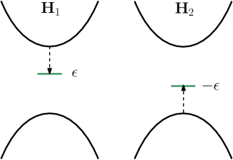
Figure 1: Illustration of evolution of midgap states of $\mathbf{H}_{1}$ and $\mathbf{H}_{2}$ branches as the twisted angle is increasing.

The scattering wavefunctions are given by

$$\psi^{S}_{\pm}(x,k)=N_{\pm}^{S}e^{ikx}\begin{pmatrix}\kappa\tanh(\kappa x)-ik\\ \pm\omega-\epsilon\end{pmatrix},$$ (20)

with eigenvalues $\pm\omega\equiv\pm\sqrt{k^{2}+\Delta_{0}^{2}}$ and normalization constant $N^{S}_{\pm}=[2L\omega(\omega\mp\epsilon)-2\kappa\tanh(\kappa L/2)]^{-1/2}$.

To determine the scattering phase shift from the kink of $\Delta(x)$, let’s first check the asymptotic behaviors of $\mathbf{H}_{1}$ as $x\rightarrow\pm\infty$

$$\mathbf{H}_{1,\pm\infty}= -i\partial_{x}\sigma_{2}\pm\kappa\sigma_{1}+\epsilon\sigma_{3}$$ (21)

which differ from each other by a SU(2) rotation $e^{i\sigma_{2}\varphi/2}$: $e^{i\sigma_{2}\varphi/2}\mathbf{H}_{1,\infty}e^{-i\sigma_{2}\varphi/2}=\mathbf{H}_{1,-\infty}$. For convenience, we denote the asymptotic wavefunction by $\psi^{S}_{\pm\infty}(x)$ at $\pm\infty$. Note that $e^{i\sigma_{2}\varphi/2}\psi^{S}_{\infty}(x)$ is an eigenstate of $\mathbf{H}_{1,-\infty}$, thus it only differs from $\psi^{S}_{-\infty}(x)$ by a phase shift $\delta(k)$, namely,

$$e^{i\sigma_{2}\varphi/2}\psi^{S}_{\infty}(x,k)=e^{i\delta(k)}\psi^{S}_{-\infty}(x,k).$$ (22)

Such a definition of phase shift has also been adopted for the $Z_{2}$ kink in the polyacetylene in Ref. Kivelson et al., 1982 together with its physical consequences.

Using the scattering wavefunctions Eq. (20), we obtain the phase shift as follows:

$$\delta^{(+)}(k)= \pi-\operatorname{atan}\frac{k}{\kappa}-\operatorname{atan}\frac{\epsilon k}{\omega\kappa},$$

for the conduction band,

$$\delta^{(-)}(k)= -\operatorname{atan}\frac{k}{\kappa}+\operatorname{atan}\frac{\epsilon k}{\omega\kappa},$$

for the valence band, (23)

as given previously in Ref. Shei, 1976. The phase shift Eq. (II.2) is useful for calculating the soliton energy and the fractional spin density distribution.

For $\mathbf{H}_{2}$, since $\mathbf{H}_{2}=-\sigma_{2}\mathbf{H}_{1}\sigma_{2}$, its eigenfunctions are simply $\sigma_{2}\psi^{B}$ and $\sigma_{2}\psi^{S}$ with opposite eigenvalues of those of $\mathbf{H}_{1}$.

II.3 Soliton energy

The groundstate energy of the uniform BCS state is divergent as the momentum cutoff $\Lambda\rightarrow\infty$, and this divergence persists in the presence of a soliton. However the difference of these energies is finite and may be defined as the excitation energy of the soliton mode. There are two contributions to the soliton energy, one is the readjustment of the fermionic spectra in the presence of the soliton, the other is the modification of the condensate energy.

To calculate the excitation energy of the soliton we follow the method given in Refs. Dashen et al., 1975 and Shei, 1976. The basic idea is to discretize the pseudo-momentum $k$ by putting the system into a box with length $L$ which is required to be much larger than the soliton size, i.e., $L\gg\kappa^{-1}$, and imposing the boundary condition Eq. (16). Thus, it is possible to make a one-to-one correspondence between the spectra of the uniform state and those of the soliton state. In the homogeneous state without the phase shift, the quantized momentum takes the values of $k_{n}=2n\pi/L$. When the twisted angle $\varphi$ is turned on adiabatically starting from zero, the pseudo-momentum $\bar{k}_{n}$ is shifted from $k_{n}=2n\pi/L$ and satisfies

$$\bar{k}^{(\pm)}_{n}L+\delta^{(\pm)}(\bar{k}^{(\pm)}_{n})=k_{n}L,$$ (24)

where the phase shifts $\delta^{(\pm)}(k)$ are given in Eq. (II.2). Therefore, the energy for each pseudo-momentum in the presence of the soliton is shifted from that in the uniform state. It is then straightforward to calculate the soliton energy by collecting the energy shifts for all the pseudo-momenta within the momentum cutoff; it is given by

$$E_{s}(\Lambda)=\frac{2\omega_{c}}{\pi}\operatorname{atan}\frac{\kappa}{\Lambda}+\frac{2\epsilon}{\pi}\operatorname{atan}\frac{\Lambda\epsilon}{\kappa\omega_{c}}-|\epsilon|$$

$$\lim_{\Lambda\rightarrow\infty}E_{s}(\Lambda)=\frac{2\kappa}{\pi}+\frac{2\epsilon}{\pi}\operatorname{atan}\frac{\epsilon}{\kappa}-|\epsilon|,$$ (25)

where $\omega_{c}=\sqrt{\Lambda^{2}+\Delta_{0}^{2}}$. If $\varphi=\pi$, we obtain the well known result $E_{s}(\infty)=2\Delta_{0}/\pi$ for the Jackiw-Rebbi soliton.

II.4 Fractional spin excitations

We introduce two local spin density operators as follows:

$$\hat{s}_{1}(x)=\hat{R}^{\dagger}_{\uparrow}\hat{R}_{\uparrow}-\hat{L}^{\dagger}_{\downarrow}\hat{L}_{\downarrow},\hskip 5.69046pt\hat{s}_{2}(x)=\hat{L}^{\dagger}_{\uparrow}\hat{L}_{\uparrow}-\hat{R}^{\dagger}_{\downarrow}\hat{R}_{\downarrow},$$ (26)

which corresponds to the two pairing branches, respectively. The expectation values of $\hat{s}_{1,2}$ denoted by $s_{1,2}(x)$ can be expanded in terms of the eigenmodes,

$$s_{1}(x)= \sum_{n}\langle\hat{d}^{\dagger}_{1n}\hat{d}_{1n}\rangle|\phi_{n}(x)|^{2}-\frac{1}{2}\sum_{n}|\phi_{n}(x)|^{2},$$ (27)

$$s_{2}(x)= \sum_{n}\langle\hat{d}^{\dagger}_{2n}\hat{d}_{2n}\rangle|\phi_{n}(x)|^{2}-\frac{1}{2}\sum_{n}|\phi_{n}(x)|^{2}.$$ (28)

In Eqs. (27) and (28), the $\phi_{n}$’s can be replaced by the orthonormal wavefunctions $\psi_{n}$’s since $\phi_{n}$’s are related to $\psi_{n}$’s by a unitary transformation. The summations in the equations above would diverge without cutoff, hence we regulate them by introducing an UV momentum cutoff $\Lambda$ chosen in such a way that in the homogeneous state there are $2N+1$ energy eigenstates for both the valence and the conduction bands. Thus in the homogeneous state, the second term in Eqs.  (27) and (28) is equal to $-(2N+1)/L$. In the presence of the soliton, this term still has a leading contribution $-(2N+1)/L$ in an expansion in the inverse powers of $L$ as shown in the appendix A, as long as we keep track of each quantum state in the process of increasing $\varphi$.

We now calculate $s_{1}(x)$ by assuming that all the scattering states in the valence band are occupied. The midgap state of the $\hat{\mathcal{H}}_{1}$-branch is left empty since it is connected to the bottom state in the conduction band and remains empty in the adiabatic process of increasing the twisted phase angle $\varphi$. The spin density $s_{1}(x)$ is then given by

$$s_{1}(x)= \sum_{n}|\psi^{S}_{-}(x,\bar{k}^{(-)}_{n})|^{2}-\frac{2N+1}{L}.$$ (29)

Clearly, the total spin number $\int_{-L/2}^{L/2}dxs_{1}(x)=0$, since the eigenstates are normalized. This agrees with the conservation law of the total spin in the adiabatic process of tuning the phase $\varphi$ of $\Delta(x)$ away from the uniform BCS state in a finite system, since the mean-field Hamiltonian always commute with the total spin operator irrespective of the specific form of $\Delta(x)$. Any kind of excitations upon this groundstate creates an integer number of spins. This results in a puzzle: can we get a fractional excitation in a finite system, while still respecting the conservation law of fermion number? The answer is yes, as we show below by calculating the local spin density $s_{1}(x)$ the exact orthonormal wavefunctions followed by an expansion with respect to $1/L$ for large enough $L$.

Substituting Eq. (20) into Eq. (29) and considering the allowed $\bar{k}_{n}$ given by Eq. (24), one finds that, up to higher order terms, the spin density $s_{1}(x)$ in fact consists of two parts, a uniform term $s_{1u}$ and a localized term $s_{1l}$:

$$s_{1}(x)=s_{1u}+s_{1l}(x)\;,$$

$$s_{1u}=\frac{c}{L}\;,$$

$$s_{1l}(x)=-\frac{c\kappa}{2}\operatorname{sech}^{2}(\kappa x)\;,$$ (30)

where $c\equiv\varphi/(2\pi)$. The detailed calculation is given in the appendix A.

Eq. (II.4) implies that, if one can measure the spin density with spatial resolution high enough, a localized spin distribution will be found around the origin($x=0$) carrying a fractional spin number $-c$ with density profile described by $s_{1l}(x)$, while the uniform one $s_{1u}$ can be ignored in this local measurement, being $O(1/L)$. Thus, it is legitimate to identify the fractional excitation as the localized density profile $s_{1l}(x)$ in a finite system. Since the thermodynamic limit is taken on local correlators for the infinite volume, the uniform term $s_{1u}$ completely disappears and we get a true fractional charge, in agreement with the results of Refs.Jackiw and Rebbi, 1976 and Fröhlich and Marchetti, 1988. The contribution of $s_{1u}$, which compenstates that of the localized term $s_{1l}$ after integration, however, can not be ignored in the discussion of the conservation of the total quantum number in finite systems.

In Eq. (29), $s_{1}(x)$ is calculated with the midgap state unoccupied and shows a localized spin distribution with a fractional quantum number $-c$. If the midgap state is filled, the localized spin density becomes $(1-c)\kappa\operatorname{sech}^{2}(\kappa x)/2$ with fractional quantum number $1-c$. If $c=1/2$, one recovers the well known result for the Jackiw-Rebbi soliton: the soliton mode carries $\pm 1/2$ charge depending on whether the zero energy state is filled or not. For general $c$, the particle-hole symmetry is broken.

Usually, one uses the arguments with fermion doubling or multiple soliton (antisoliton) excitations to resolve the issue concerning the compatibility of the emergence of the fractional fermion number with the conservation of the integer number of the elementary constituent fermions. Here, we provide a new and more fundamental perspective to this issue that a single localized soliton mode carrying a fractional quantum number can exist independently (in the sense specified above) in a one-dimensional finite system compenstated by an opposite fractional charge distributed uniformly in the background.

Similarly one can compute the spin density $s_{2}(x)$ of the other pairing branch. Note that the wavefunctions of the valence band of $\hat{\mathcal{H}}_{2}$ are $\sigma_{2}\psi^{(+)}(x,\bar{k}^{(+)}_{n})$, and the midgap state is $\sigma_{2}\psi^{B}(x)$, which evolves from the state on the top of the valence band and is assumed to be occupied as we tune the phase $\varphi$ adiabatically. Then, we obtain

$$s_{2}(x)=\sum_{n}|\psi^{S}_{+}(x,\bar{k}_{n})|^{2}+|\psi^{B}(x)|^{2}-\frac{2N+1}{L}.$$ (31)

As shown in the appendix  A, to the leading order, $s_{2}(x)$ can be recast as

$$s_{2}(x)=s_{2u}+s_{2l}(x),$$

$$s_{2u}=-\frac{c}{L},$$

$$s_{2l}=\frac{\kappa c}{2}\operatorname{sech}^{2}(\kappa x).$$ (32)

Again, we observe a localized fractional excitation $s_{2l}$ and a uniform background $s_{2u}$. They cancel with each other after integration respecting the spin conservation law in a finite system.

Although there are fractional excitations for each branch individually, their sum is trivial $s_{1}(x)+s_{2}(x)=0$ consistent with the result for the uniform BCS state. In fact, there are four cases with different spin number depending on the configurations of the midgap states as follows: spin 1 for both filled, spin 0 for half filling with two cases, and spin -1 for both empty, all of which carry an integer spin number instead of a fractional one. Thus, the fermion doubling dispels the fractional excitation. To get the fractional spin excitations, one needs to avoid the fermion doubling. Note that the edge mode of a quantized spin Hall insulator consists of only one branch of Dirac fermionKane and Mele (2005); Bernevig et al. (2006), if it is coupled to a superconductor appropriately, the proximity effect may induce a one-dimensional superconductor without fermion doubling which may be a possible candidate to observe the fractional spin excitation.

III Majorana zero mode in $p$ wave superfluid

In this section, we consider the soliton mode in one-dimensional $p$-wave superconductors with only one species of fermions with the following minimal HamiltonianRead (2000); Sengupta et al. (2001)

$$\hat{H}= -\int dx\mu(x)\hat{c}^{\dagger}(x)\hat{c}(x)$$

$$-\frac{1}{2}\int dx\left[\hat{c}^{\dagger}(x)i\partial_{x}\hat{c}^{\dagger}(x)+\hat{c}(x)i\partial_{x}\hat{c}(x)\right]$$ (33)

where $\hat{c}(x)$ and $\hat{c}^{\dagger}(x)$ are the spinless annhilation and creation operators. The chemical potential $\mu(x)=\mu_{0}\tanh(\mu_{0}x)$ with $\mu_{0}>0$, interpolates between the weak and strong pairing phases. This Hamiltonian resembles the Jackiw-Rebbi model, and a $Z_{2}$ soliton mode occurs which turns out to be a Majorana zero mode.

The Hamiltonian Eq. (III) can be diagonalized as

$$\hat{H}=\sum_{k}\omega_{k}\hat{d}_{k}^{\dagger}\hat{d}_{k}+\text{const.}$$ (34)

where $\omega_{k}=\sqrt{k^{2}+\mu_{0}^{2}}$ for the scattering state with $k\neq 0$, and $\omega_{0}=0$ for the zero mode. The quasi-particle operator $\hat{d}_{k}$ is a linear combination of $\hat{c}(x)$ and $\hat{c}^{\dagger}(x)$ given by

$$\hat{d}_{k}=\int dx[u^{*}_{k}(x)\hat{c}(x)+v_{k}(x)\hat{c}^{\dagger}(x)].$$ (35)

The wavefunction $\phi(x,k)\equiv[u^{*}_{k}(x),v_{k}(x)]^{t}$ satisfies the following equation

$$\mathcal{H}\phi(x,k)\equiv[-\mu(x)\sigma_{3}+i\partial_{x}\sigma_{1}]\phi(x,k)=\omega_{k}\phi(x,k).$$ (36)

Note that since $\sigma_{1}\mathcal{H}^{*}\sigma_{1}=-\mathcal{H}$, the state $\sigma_{1}\phi^{*}(x,k)$ has a negative energy $-\omega_{k}$ and the corresponding annihilation operator is simply the Hermitean conjugate of $\hat{d}_{k}$. Therefore, one need only take the positive energy states into account.

In a finite system of length $L$ the energy eigenfunctions consist of a localized zero mode, given, up to a rest exponentially small in $L$, by

$$\phi^{B}(x)= \frac{e^{-i\pi/4}\sqrt{\mu_{0}}}{2}\operatorname{sech}(\mu_{0}x)\begin{pmatrix}1\\ i\end{pmatrix},$$ (37)

and of the scattering wavefunctions

$$\phi^{S}(x,k)=\frac{1}{N_{k}}e^{-i\pi/4}e^{ikx}\begin{pmatrix}\mu(x)-ik-\omega\\ i\mu(x)+k+i\omega\end{pmatrix},$$ (38)

with the normalization constant $N_{k}=2\sqrt{L\omega_{k}^{2}-\mu(L/2)}$. The global phase factor $e^{-i\pi/4}$ is taken for convenience. Eq. (37) shows that $u_{0}(x)=v_{0}(x)$, which indicates that $\hat{d}_{0}$ is actually a Majorana zero mode, while $\hat{d}_{k}$ is a normal Fermi operator for the scattering solution with $k\neq 0$.

Since the chemical potential has opposite signs at the two ends, a particle excitation at one end could be a hole excitation at the other end. This allows us to choose the boundary condition for a finite system as

$$\sigma_{1}\phi^{S}(L/2,k)=\phi^{S}(-L/2,k).$$ (39)

Note that the inverse transformation of Eq. (35) gives rise to the spinless fermion operator in terms of $\hat{d}_{k}$ as

$$\hat{c}(x)= u_{0}(x)\hat{d}_{0}+\sum_{\bar{k}}u_{\bar{k}}(x)\hat{d}_{\bar{k}}+v_{\bar{k}}(x)\hat{d}^{\dagger}_{\bar{k}}.$$ (40)

As long as $L\gg\mu_{0}^{-1}$, $u_{0}(\pm L/2)\rightarrow 0$, and the boundary condition Eq. (39) is equivalent to $c(L/2)=c^{\dagger}(-L/2)$.

As in the $s$-wave pairing case, one can not define the phase shift directly, because the asymptotic Hamiltonian as $x\rightarrow\pm\infty$ are not equal, instead they are related to each other by $\sigma_{1}\mathcal{H}_{-\infty}\sigma_{1}=\mathcal{H}_{\infty}$. Therefore, the phase shift can be defined as $e^{i\delta(k)}\phi^{S}_{-\infty}(x,k)=\sigma_{1}\phi^{S}_{\infty}(x,k)$, where $\phi_{\pm\infty}^{S}(x,k)$ are the asymptotic wavefunction as $x\rightarrow\pm\infty$, and it can be calculated as

$$\delta(k)=-\pi/2-\operatorname{atan}(k/\mu_{0}).$$ (41)

For a finite system, the allowed pseudo-momentum is determined by the boundary condtion Eq. (39) and the phase shift Eq. (41).

Since in the $p$-wave pairing phase, the global U(1) symmetry is broken down to $Z_{2}$, the fermion number is not a conserved quantity anymore, but its parity is still conserved. On the other hand, the dimension of the Hilbert space should keep the same, no matter how the annihilation and creation operators are mixed. It also does not change with the chemical potential as long as we make a one-to-one correspondence of the allowed pseudo-momenta for different $\mu_{0}$ and impose the same boundary condition Eq. (39). Therefore, we suggest that the fractionalized quantum number of the soliton in the $p$-wave pairing superconductor is the the “dimension” of its single particle Hilbert space, defined via a suitably renormalized the trace of the identity.

For this purpose, with an UV momentum cutoff $\Lambda$ chosen as before, we introduce the concept of the dimension density $D(x)$ of the single particle Hilbert space as the sum over the modulus square of all the energy eigenfunctions up to the cutoff, i.e. the diagonal of the resolution of the identity for the energy in the $x$-representation. It follows that the integral of $D(x)$ is the total dimension of the Hilbert space, or, equivalently, the number of the allowed pseudo-momenta plus the number of localized zero modes, denoted by $N_{D}$ and it is invariant against adiabatic changes of the chemical potential. In our model with the soliton mode

$$D(x)=|\phi^{B}(x)|^{2}+\sum_{\bar{k}}|\phi^{S}(x,\bar{k})|^{2}.$$ (42)

Its integral diverges in the limit of infinite cutoff $\Lambda$, but the difference with respect to the same quantity in the absence of the $Z_{2}$ soliton is finite and independent of the cutoff.

For a normal system with fermion number conserved $D(x)$ is uniform and equal to $N_{D}/L$, since after all $D(x)$ is just the fermion density with all the single particles states occupied. However, $D(x)$ is not uniform in the present system with a localized Majorana zero mode (in a sense only one half of the Jackiw-Rebbi model). Following a procedure similar to that given in the appendix, we find in presence of the soliton

$$D(x)-\frac{N_{D}}{L}=\frac{1}{2}|\phi_{B}(x)|^{2}-\frac{1}{2L}+o(L^{-2}).$$ (43)

We observe that there is a localized term which carries $1/2$ factor indicating 1/2 dimension of the single particle Hilbert space. Once integrated over the whole space, it can be cancelled by the next uniform term in the r.h.s. of Eq. (43), leaving the total dimension of the single particle Hilbert space invariant. In the thermodynamic limit $L\rightarrow\infty$, the uniform term is unobservable leaving a point-like Majorana zero mode with “dimension” $\delta=1/2$, thus obeying exclusion statistics with parameter 1/2Haldane (1991); Ye et al. (2015, 2017). Furthermore the total Hilbert space of $N$ fermion modes has dimension $2^{N}$, but according to the above calculation the total Hilbert space of $N$ soliton modes has dimension $2^{\delta N}$, so that their quantum dimension is $2^{\delta}=\sqrt{2}$, intriguingly coinciding with the quantum dimension of Majorana vortex mode in a topological superconductorNayak et al. (2008); Kitaev (2006).

It should be emphasized that the spatial dependence of $D(x)$ given in Eq. (43) is not at all obvious; this may be closely related to the nonlocal nature of the topological Majorana type excitations, and also distinguishes the Majorana zero mode from other one-dimensional topological excitations. For example, one can calculate the dimension density for the complex $Z_{2}$ soliton models, and it turns out to be $D(x)-N_{D}/L=0$ (see the appendix) implying a quantum dimension $2^{0}=1$ of the complex $Z_{2}$ soliton mode. Such a result is also in agreement of the quantum dimension of abelian anyonsKitaev and Preskill (2006) (note that these solitons are connected to the anyonic excitations in the fractional quantum Hall effectLee et al. (2007)). Given all these coincidences, however, it is still lacking a clear connection between the ”dimension” defined through a renormalized trace of the identity, as done above, and the quantum dimension.

IV Conclusion

As a summary, we consider the soliton mode emerging in one-dimensional superconductors which are closely related to the fractional quasiparticles in the two dimensional systems using the idea of edge soliton as given in Ref.Lee et al., 2007.

For $s$-wave pairing, the phase of the order parameter is twisted by $\pm\varphi/2$ at the two ends. The mean-field Hamiltonian is analogous to the Jackiw-Rebbi model, suggesting the existence of fractional spin excitations. Indeed, by solving the corresponding BdG equation, we find a single complex $Z_{2}$ soliton mode carrying a fractional spin number $c=\varphi/(2\pi)$, although the fermion doubling conceals this fractional excitation. Using the exact wavefunctions in the presence of a complex $Z_{2}$ soliton, we expand the spin density in a system of length $L$ with respect to $L^{-1}$ and find that it consists of two parts, a localized spin density profile with a fractional number $c$ and a uniform spin density $-c/L$. The uniform distribution disappears in the thermodynamic limit, but it is essential to keep the spin number conserved for a finite system. Our analysis is applicable to other one-dimensional systems with fractional excitations such as the Jackiw-Rebbi model with particle number conserved, thus provides a mechanism to solve the puzzle of the emergence of the fractional fermion number in a finite system with conserved integral quantum number.

For $p$-wave pairing with chemical potential interpolating between the strong and weak pairing phase, the emergent $Z_{2}$ soliton mode is of the Majorana type. By introducing the concept of dimension density of the single particle Hilbert space, we associate the Majorana zero mode with 1/2 dimension of the single particle Hilbert space, which suggests that it may be understood as an object with 1/2 exclusion statisticsHaldane (1991); Ye et al. (2015, 2017). This result also suggests a dimension of $\sqrt{2}$ in the total Hilbert space which agrees with the quantum dimension of the Majorana vortex in a two-dimensional $p$-wave superconductor. Similar calculations can also be performed for the complex $Z_{2}$ soliton, it turns out to be $2^{0}=1$ coinciding with the quantum dimension of abelian anyonsKitaev and Preskill (2006).

Finally, strictly speaking the mean-field treatment may not be accurate for one-dimensional interacting fermions where the Luttinger liquid theory may be more appropriate. However as shown in Ref.Fröhlich and Marchetti, 1988, the interaction does not interfere with the appearance of a fractional charge and this suggests that the argument given in this article can be extended to the framework of Luttinger liquids.

Appendix A Derivation of spin density in space

We introduce the following three terms

$$\tilde{s}_{m}(x)= \frac{\kappa}{2}\operatorname{sech}^{2}(\kappa x),$$

$$\tilde{s}_{-}(x)= \sum_{n}|\psi^{S}_{-}(x,\bar{k}^{(-)}_{n})|^{2},$$

$$\tilde{s}_{+}(x)= \sum_{n}|\psi^{S}_{+}(x,\bar{k}^{(+)}_{n})|^{2},$$ (44)

which correspond to the midgap state, valence band and conduction band of $\mathcal{H}_{1}$. They are connected with $s_{1}(x)$ and $s_{2}(x)$ defined in Sec. II.4 as $s_{1}(x)=\tilde{s}_{-}(x)$ and $s_{2}(x)=\tilde{s}_{m}(x)+\tilde{s}_{+}(x)$.

Using Eq. (20), we find

$$|\psi^{S}_{\pm}(x,k)|^{2}= \frac{\kappa^{2}\tanh^{2}(\kappa x)+k^{2}+(\omega+\epsilon)^{2}}{2L\omega(\omega\mp\epsilon)-2\kappa\tanh(\kappa L/2)}$$

$$= \frac{1}{L}+\frac{(2\kappa/L)-\kappa^{2}\operatorname{sech}^{2}(\kappa x)}{2L\omega(\omega+\epsilon)-2\kappa}+o(e^{-\kappa L}),$$

then

$$\tilde{s}_{\pm}(x)= \frac{\mathcal{N}_{\pm}}{L}+\sum_{n}\frac{(2\kappa/L)-\kappa^{2}\operatorname{sech}^{2}(\kappa x)}{2L\omega(\omega\mp\epsilon)-2\kappa}$$

$$= \frac{\mathcal{N}_{\pm}}{L}+\frac{L}{2\pi}\int d\bar{k}\frac{(2\kappa/L)-\kappa^{2}\operatorname{sech}^{2}(\kappa x)}{2L\omega(\omega\mp\epsilon)-2\kappa}$$

$$\hskip 85.35826pt\times\left(1+\frac{1}{L}\frac{\partial\delta^{(\pm)}(\bar{k})}{\partial\bar{k}}\right)$$

where $\mathcal{N}_{\pm}$ is the number of the allowed momenta in the conduction and valence bands, respectively. Since the midgap state is lowered down from the conduction band, $\mathcal{N}_{+}=2N/L$ and $\mathcal{N}_{-}=(2N+1)/L$.

Using the identity

$$\frac{\kappa}{\pi}\int_{0}^{\infty}dk\frac{1}{\omega(\omega+\epsilon)}=\frac{\varphi}{2\pi}\equiv c,$$ (45)

we finally obtain

$$\tilde{s}_{+}(x)= \frac{2N+1-c}{L}-\frac{(1-c)\kappa}{2}\operatorname{sech}^{2}(\kappa x)+o(L^{-1}),$$

$$\tilde{s}_{-}(x)= \frac{2N+1+c}{L}-\frac{c\kappa}{2}\operatorname{sech}^{2}(\kappa x)+o(L^{-1}).$$ (46)

In the presence of soliton, $\tilde{s}_{-}(x)+\tilde{s}_{+}(x)+\tilde{s}_{m}(x)=\frac{2(2N+1)}{L}$ by ignoring the higher order terms, which is just $\sum_{n}|\phi_{n}(x)|^{2}$ in Eqs. (27) and (28) and also the dimension density $D(x)$ defined for these system(see Eq. (42)).

References

- Su et al. (1980) W. P. Su, J. R. Schrieffer, and A. J. Heeger, Phys. Rev. B 22, 2099 (1980).
- Laughlin (1983) R. B. Laughlin, Phys. Rev. Lett. 50, 1395 (1983).
- Read (2000) N. Read, and D. Green, Phys. Rev. B 61, 10267 (2000).
- Sengupta et al. (2001) K. Sengupta, I. Žutić, H.-J. Kwon, V. M. Yakovenko, and S. Das Sarma, Phys. Rev. B 63, 144531 (2001).
- Kitaev (2001) A. Y. Kitaev, Phys. Usp. 44 (2001).
- Ye et al. (2002) F. Ye, G. H. Ding, and B. W. Xu, Commun. Theor. Phys. 37, 492 (2002).
- Ye and Xu (2003) F. Ye and B. W. Xu, Commun. Theor. Phys. 39, 487 (2003).
- Jackiw and Rebbi (1976) R. Jackiw and C. Rebbi, Phys. Rev. D 13, 3398 (1976).
- Qi et al. (2008) X.-L. Qi, T. L. Hughes, and S.-C. Zhang, Nature Physics 4, 273 (2008).
- Fröhlich and Marchetti (1988) J. Fröhlich and P. Marchetti, Communications in Mathematical Physics 116, 127 (1988).
- Jackiw and Schrieffer (1981) R. Jackiw and J. R. Schrieffer, Nuclear Physics B 190, 253 (1981), ISSN 0550-3213.
- Strocchi (2008) F. Strocchi, Symmetry Breaking, Lecture Notes in Physics 732 (Springer-Verlag Berlin Heidelberg, 2008), 2nd ed.
- Fulde and Ferrell (1964) P. Fulde and R. A. Ferrell, Phys. Rev. 135, A550 (1964).
- Larkin and Ovchinnikov (1965) A. I. Larkin and Y. N. Ovchinnikov, Sov. Phys. JETP 20, 762 (1965).
- Yang (2001) K. Yang, Phys. Rev. B 63, 140511(R) (2001).
- Orso (2007) G. Orso, Phys. Rev. Lett. 98, 070402 (2007).
- Hu et al. (2007) H. Hu, X.-J. Liu, and P. D. Drummond, Phys. Rev. Lett. 98, 070403 (2007).
- Feiguin and Heidrich-Meisner (2007) A. E. Feiguin and F. Heidrich-Meisner, Phys. Rev. B 76, 220508(R) (2007).
- Rizzi et al. (2008) M. Rizzi, M. Polini, M. A. Cazalilla, M. R. Bakhtiari, M. P. Tosi, and R. Fazio, Phys. Rev. B 77, 245105 (2008).
- Tezuka and Ueda (2008) M. Tezuka and M. Ueda, Phys. Rev. Lett. 100, 110403 (2008).
- Ye et al. (2009) F. Ye, Y. Chen, Z. D. Wang, and F. C. Zhang, Journal of Physics: Condensed Matter 21, 355701 (2009).
- Yanase (2009) Y. Yanase, Phys. Rev. B 80, 220510 (2009).
- Liao et al. (2010) Y.-a. Liao, A. S. C. Rittner, T. Paprotta, W. Li, G. B. Partridge, R. G. Hulet, S. K. Baur, and E. J. Mueller, Nature 467, 567 (2010).
- Mourik et al. (2012) V. Mourik, K. Zuo, S. M. Frolov, S. R. Plissard, E. P. A. M. Bakkers, and L. P. Kouwenhoven, Science 336, 1003 (2012), ISSN 0036-8075.
- Das et al. (2012) A. Das, Y. Ronen, Y. Most, Y. Oreg, M. Heiblum, and H. Shtrikman, Nat Phys 8, 887 (2012).
- Finck et al. (2013) A. D. K. Finck, D. J. Van Harlingen, P. K. Mohseni, K. Jung, and X. Li, Phys. Rev. Lett. 110, 126406 (2013).
- Churchill et al. (2013) H. O. H. Churchill, V. Fatemi, K. Grove-Rasmussen, M. T. Deng, P. Caroff, H. Q. Xu, and C. M. Marcus, Phys. Rev. B 87, 241401 (2013).
- Deng et al. (2012) M. T. Deng, C. L. Yu, G. Y. Huang, M. Larsson, P. Caroff, and H. Q. Xu, Nano Letters 12, 6414 (2012).
- Albrecht et al. (2016) S. M. Albrecht, A. P. Higginbotham, M. Madsen, F. Kuemmeth, T. S. Jespersen, J. Nygrd, P. Krogstrup, and C. M. Marcus, Nature 531, 206 (2016), letter.
- Nayak et al. (2008) C. Nayak, S. H. Simon, A. Stern, M. Freedman, and S. Das Sarma, Rev. Mod. Phys. 80, 1083 (2008).
- Goldstone and Wilczek (1981) J. Goldstone and F. Wilczek, Phys. Rev. Lett. 47, 986 (1981).
- MacKenzie and Wilczek (1984) R. MacKenzie and F. Wilczek, Phys. Rev. D 30, 2194 (1984).
- Frolov (1972) I. S. Frolov, Sov. Math. Dokl. 13, 1468 (1972).
- Dashen et al. (1975) R. F. Dashen, B. Hasslacher, and A. Neveu, Phys. Rev. D 12, 2443 (1975).
- Shei (1976) S.-S. Shei, Phys. Rev. D 14, 535 (1976).
- H.Grosse and G.Opelt (1987) H.Grosse and G.Opelt, Nucl. Phys. B 285, 143 (1987).
- Kivelson et al. (1982) S. Kivelson, T.-K. Lee, Y. R. Lin-Liu, I. Peschel, and L. Yu, Phys. Rev. B 25, 4173 (1982).
- Kane and Mele (2005) C. L. Kane and E. J. Mele, Phys. Rev. Lett. 95, 146802 (2005).
- Bernevig et al. (2006) B. A. Bernevig, T. L. Hughes, and S.-C. Zhang, Science 314, 1757 (2006).
- Haldane (1991) F. D. M. Haldane, Phys. Rev. Lett. 67, 937 (1991).
- Ye et al. (2015) F. Ye, P. A. Marchetti, Z. B. Su, and L. Yu, Phys. Rev. B 92, 235151 (2015).
- Ye et al. (2017) F. Ye, P. A. Marchetti, Z. B. Su, and L. Yu, J. Phys. A: Math. Theor. 50, 395401 (2017).
- Kitaev (2006) A. Kitaev, Annals of Physics 321, 2 (2006), ISSN 0003-4916, january Special Issue.
- Kitaev and Preskill (2006) A. Kitaev and J. Preskill, Phys. Rev. Lett. 96, 110404 (2006).
- Lee et al. (2007) D.-H. Lee, G.-M. Zhang, and T. Xiang, Phys. Rev. Letts. 99, 196805 (pages 4) (2007).