Probing large scale homogeneity and periodicity in the LRG distribution using Shannon entropy

Abstract

We quantify the degree of inhomogeneity in the Luminous Red Galaxy (LRG) distribution from the SDSS DR7 as a function of length scales by measuring the Shannon entropy in independent and regular cubic voxels of increasing grid sizes. We also analyze the data by carrying out measurements in overlapping spheres and find that it suppresses inhomogeneities by a factor of $5$ to $10$ on different length scales. Despite the differences observed in the degree of inhomogeneity both the methods show a decrease in inhomogeneity with increasing length scales which eventually settle down to a plateau at $\sim 150\,h^{-1}\rm{Mpc}$. Considering the minuscule values of inhomogeneity at the plateaus and their expected variations we conclude that the LRG distribution becomes homogeneous at $150\,h^{-1}\rm{Mpc}$ and beyond. We also use the Kullback-Leibler divergence as an alternative measure of inhomogeneity which reaffirms our findings. We show that the method presented here can effectively capture the inhomogeneity in a truly inhomogeneous distribution at all length scales. We analyze a set of Monte Carlo simulations with certain periodicity in their spatial distributions and find periodic variations in their inhomogeneity which helps us to identify the underlying regularities present in such distributions and quantify the scale of their periodicity. We do not find any underlying regularities in the LRG distribution within the length scales probed.

1 Introduction

Statistical homogeneity and isotropy of the Universe on sufficiently large scales is a crucial assumption which simplifies the study of large scale structure of the Universe and Cosmology as a whole. This assumption which is known as the cosmological principle is one of the fundamental pillars of modern cosmology. One can not derive this principle in a strictly mathematical sense and can only verify this by analyzing various cosmological observations and comparing them with the theoretical predictions based on it. So far the most compelling evidence of isotropy comes from the near uniform temperature of the CMBR over the full sky (Penzias & Wilson, 1965; Smoot et al., 1992; Fixsen et al., 1996). This is further supported by multitude of evidences such as the isotropy in angular distributions of radio sources (Wilson & Penzias, 1967; Blake & Wall, 2002), isotropy in the X-ray background (Peebles, 1993; Wu et al., 1999; Scharf et al., 2000), isotropy of Gamma-ray bursts (Meegan et al., 1992; Briggs et al., 1996), isotropy in the distribution of galaxies (Marinoni et al., 2012; Alonso et al., 2015), isotropy in the distribution of supernovae (Gupta & Saini, 2010; Lin et al., 2015) and isotropy in the distribution of neutral hydrogen (Hazra & Shafieloo, 2015). But merely having isotropy around us does not guarantee homogeneity of the Universe. One can infer homogeneity from isotropy only when it is assured around each and every point with the hypothesis that the matter distribution is a smooth function of position (Straumann, 1974; Sylos Labini & Baryshev, 2010). Unfortunately even the isotropy of the Universe around us is not certain as there are mounting evidences in favour of significant anisotropy in the Universe. The CMBR which is considered to be the best supporting evidence for isotropy is not completely isotropic. Over the years many studies have reported power asymmetries and unlikely alignments of low multipoles (Schwarz et al., 2004; Land & Magueijo, 2005; Hanson & Lewis, 2009; Moss et al., 2011; Gruppuso et al., 2013; Dai et al., 2013). Recently Planck Collaboration et al. (2014) reported a $3-\sigma$ deviations from isotropy in the PLANCK data. There are other studies such as the hemispherical asymmetry of cosmological parameters (Jackson, 2012; Bengaly et al., 2015), shape of the luminosity function of galaxies (Appleby & Shafieloo, 2014), Hubble diagram of Type Ia Supernovae (Schwarz & Weinhorst, 2007; Kalus et al., 2013), redshift-magnitude relation of Type Ia Supernovae (Javanmardi et al., 2015) which find significant evidence for anisotropy. As a result it is not straightforward to infer homogeneity of the Universe by combining isotropy with the Copernican principle.

Most statistical tests to identify the transition scale to homogeneity rely on the number counts $n(<r)$ in spheres of radius $r$ and its scaling with $r$ which is expected to scale as $\sim r^{3}$ for a homogeneous distribution. The conditional density (Hogg et al., 2005; Sylos Labini, 2011a) measures the average density in these spheres which is expected to flatten out beyond the scale of homogeneity. The multifractal analysis (Martinez & Jones, 1990; Coleman & Pietronero, 1992; Borgani, 1995) uses the scaling of different moments of $n(<r)$ to characterize the scale of homogeneity. Some of the studies carried out so far with these methods on different galaxy surveys claim to have found a transition to homogeneity on sufficiently large scales $70-150\,h^{-1}\rm{Mpc}$ (Martinez & Coles, 1994; Guzzo, 1997; Martinez et al., 1998; Bharadwaj et al., 1999; Pan & Coles, 2000; Kurokawa et al., 2001; Hogg et al., 2005; Yadav et al., 2005; Sarkar et al., 2009; Scrimgeour et al., 2012; Pandey et al., 2015) whereas some studies claim the absence of any such transition out to scale of the survey (Coleman & Pietronero, 1992; Amendola & Palladino, 1999; Sylos Labini et al., 2007, 2009a, 2009b; Sylos Labini, 2011b). Bulk flow measurements on large scales provide another important test for the large scale homogeneity. The galaxy distribution as revealed by different galaxy redshift surveys (SDSS, York et al. 2000; 2dFGRS, Colles et al. 2001) indicates that the Universe is highly inhomogeneous and anisotropic on small scales. The observed deviations from homogeneity and isotropy arise from peculiar velocities resulting from density perturbations. Any form of bulk flows are expected to disappear on sufficiently large scales where the density fluctuations are very small. Analysis of a large number of peculiar velocity surveys indicate statistically significant large cosmic flows on scales of $100\,h^{-1}\,{\rm Mpc}$ (Watkins et al., 2009). Combined studies with the WMAP data and x-ray cluster catalog indicates strong and coherent bulk flow out to $\gtrsim 300\,h^{-1}\,{\rm Mpc}$ (Kashlinsky et al., 2008, 2010). Contrary to these claims a recent study of low-redshift Type-Ia Supernovae suggest no excess bulk flow on top of what is expected in $\Lambda$CDM model (Huterer et al., 2015). If large scale bulk motions really exist then they indicate that there are significant density fluctuations on very large scales. The results from these studies clearly indicate that there is no clear consensus in this issue yet. The presence of inhomogeneities on very large scales has several important consequences. Inhomogeneities, through the backreaction mechanism can provide an alternate explanation of a global cosmic acceleration without requiring any additional dark energy component (Buchert & Ehlers, 1997; Buchert, 2001; Schwarz, 2002; Kolb et al., 2006; Paranjape, 2009; Kolb et al., 2010; Ellis, 2011). Spherically symmetric radially inhomogeneous Lemaitre-Tolman-Bondi (LTB) models can account for the distant supernova data in a dust universe without requiring any dark energy (Garcia-Bellido & Haugbølle, 2008; Enqvist, 2008). A large void can also mimic an apparent acceleration of expansion (Tomita, 2001; Hunt & Sarkar, 2010). Fortunately such models can be constrained with observations such as SNe, CMB, BAO and measurements of angular diameter distance and Hubble parameter (Zibin et al., 2008; Clifton et al., 2008; Biswas et al., 2010; Clarkson, 2012; Larena et al., 2009; Valkenburg et al., 2014). There would be a major paradigm shift in cosmology if the assumption of cosmic homogeneity is ruled out with high statistical significance by multiple data sets and it is important to test the assumption of homogeneity on multiple datasets with different statistical tools.

Pandey (2013) introduce a method based on Shannon entropy (Shannon, 1948) for characterizing inhomogeneities and applied the method on some Monte Carlo simulations of inhomogeneous distributions and N-body simulations which show that the proposed method has great potential for testing the large scale homogeneity in galaxy redshift surveys. Pandey et al. (2015) applied this method to galaxy distributions from SDSS DR12 (Alam et al., 2015) and find that the inhomogeneities in the galaxy distributions persist at least upto a length scale of $120\,h^{-1}\,{\rm Mpc}$. Pandey (2013) show that the methods for testing homogeneity based on the number counts are contaminated by confinement and overlapping biases which result from the systematic migration and overlap between the spheres with increasing radii. These biases which are inevitable in any finite volume sample, artificially suppress inhomogeneities at each scale and particularly on large scales. Recently Kraljic (2015) use the count in cells method in Dark Sky simulations (Skillman et al., 2014) to show the spurious effects in the measurement of correlation dimension due to the confinement and overlapping biases. One can circumvent these biases by using number counts in independent spheres but the availability of only a very small number of independent spheres at increasing radii makes the statistics too noisy for most galaxy samples available including the SDSS Main galaxy sample. Using count in cells method as well as new methods based on anomalous diffusion and random walks Kraljic (2015) show that the Millennium Run simulation (Springel et al., 2005) volume is too small and prone to bias to reliably identify the onset of homogeneity. We require galaxy distributions covering very large volume to serve the purpose. The luminous red galaxy distribution (LRG) (Eisenstein et al., 2001) extends to a much deeper region of the Universe as compared to the SDSS Main galaxy sample as they can be observed to greater distances as compared to normal $L_{\star}$ galaxies for a given magnitude limit. Their stable colors also make them relatively easy to pick out from the rest of the galaxies using the SDSS multi-band photometry. The enormous volume covered by the SDSS LRG distribution provides us an unique opportunity to test the assumption of homogeneity on large scales with unprecedented confidence. We modify our method (Pandey, 2013) so as to carry out the analysis with non-overlapping independent regions upto sufficiently large length scales. We also analyze the LRG data with overlapping spheres and compare the findings with that obtained using independent regions to asses the suppression of inhomogeneities on different length scales due to overlapping and confinement biases.

Beside analyzing the issue of cosmic homogeneity using the LRG distribution we also address another important issue in the present work. Some studies reported to have found periodicity in the observed distribution of galaxies and galaxy clusters (Broadhurst et al., 1990; Einasto et al., 1997a). Both Broadhurst et al. (1990) and Einasto et al. (1997a) find an apparent regularity in the galaxy distribution at a characteristic length scale of $120-130\,h^{-1}\,{\rm Mpc}$. It has been suggested that in an oscillating Universe the oscillation of the Hubble parameter can cause such periodicity in the density fluctuations (Morikawa, 1990; Hirano & Komiya, 2010). Einasto et al. (1997b) use the oscillations in the cluster correlation function to quantify such pictures of regularity in the galaxy distribution. The correlation function being an isotropic statistics smooths out the anisotropic signal and may not be the best statistics to describe such anisotropic structures. Recently Pandey (2015) suggest a method which shows that Shannon entropy can be also employed to test the isotropy of a distribution. We shall use some inhomogeneous and anisotropic distributions with regularity in their distributions and test if the method presented here can describe such underlying regularities in the distributions. A recent study by Ryabinkov et al. (2013) find quasi-periodical features in the distribution of LRGs. Recently Einasto et al. (2015a) detected two peaks in the distance distributions of rich galaxy groups and clusters at $120\,h^{-1}\,{\rm Mpc}$ and $240\,h^{-1}\,{\rm Mpc}$ around the Abell cluster A2142. Another study by Einasto et al. (2015b) find evidence for shell like structures in the SDSS galaxy distribution where galaxy clusters have maxima in the distance distribution to other galaxy groups and clusters at the distance of about $120\,h^{-1}\,{\rm Mpc}$. Galaxies are distributed in a complex filamentary network which is often referred as the Cosmic web. Filaments are known to be the largest known statistically significant coherent structures in the Universe (Bharadwaj et al., 2004; Pandey & Bharadwaj, 2005; Pandey, 2010). Pandey et al. (2011) find that the filaments are statistically significant upto a length scales of $120\,h^{-1}\,{\rm Mpc}$ in the LRG distribution and longer filaments, though possibly present in the data, are not statistically significant and are the outcome of chance alignments. These studies suggest that there may be a characteristic scale present in the galaxy distribution other than the Baryon Acoustic Oscillations (BAO) feature observed at $100\,h^{-1}\,{\rm Mpc}$ (Eisenstein et al., 2005). In an earlier study Pandey et al. (2015) find that the inhomogeneities in the SDSS Main galaxy distribution persist at least upto a length scales of $120\,h^{-1}\,{\rm Mpc}$ and we would like to test if the inhomogeneities in the LRG distribution exhibit any regularity on even larger scales.

Throughout our work, we have used the flat $\Lambda$CDM cosmology with $\Omega_{m}=0.3,\;\Omega_{\Lambda}=0.7\mbox{ and }h=1$.

2 METHOD OF ANALYSIS

Pandey (2013) propose a method based on the Shannon entropy to study inhomogeneities in a 3D distribution. Shannon entropy (Shannon, 1948) is originally proposed by Claude Shannon to quantify the information content in strings of text. It gives a measure of the amount of information required to describe a random variable. The Shannon entropy for a discrete random variable $X$ with $n$ outcomes $\{x_{i}:i=1,....n\}$ is a measure of uncertainty denoted by $H(X)$ defined as,

$$H(X)=-\sum^{n}_{i=1}\,p(x_{i})\,\log\,p(x_{i})$$ (1)

where $p(x)$ is the probability distribution of the random variable $X$.

We modify the method proposed by Pandey (2013) which employs spheres of varying radii $r$ to measure the number counts inside them. The spheres are allowed to overlap which suppress inhomogeneities and the degree of overlap gradually increases with increasing radii. In order to prevent overlapping of the measuring volumes which hinders measurement of inhomogeneity on large scales we embed the galaxy distribution in a $d\,h^{-1}\,{\rm Mpc}\times d\,h^{-1}\,{\rm Mpc}\times d\,h^{-1}\,{\rm Mpc}$ three dimensional rectangular grid. This divides the entire survey region into a number of regular cubic voxels. The voxels which are beyond the boundary of the survey region are marked and discarded from the analysis. We also discard the voxels near the boundary which are partly inside the survey region to avoid any edge effects. We identify the voxels which are fully inside the survey region and only consider them in our analysis. The grid size $d$ is a variable which can be varied within a suitable range. Each choice of $d$ would result into a different number of analyzable voxels and galaxies within the survey region. Let $N_{d}$ be the number of resulting voxels which lie entirely within the survey region for a grid size $d$. We count the number of galaxies inside each of the $N_{d}$ voxels available for each choice of grid size $d$. Let $n_{i}$ be the number counts inside the $i^{th}$ voxel where the voxel index $i$ runs from $1$ to $N_{d}$. In general for a specific choice of the grid size if we randomly pick up a galaxy it can reside only in one of the $N_{d}$ voxels available for that $d$. But which particular voxel does it belong to ? The answer to this question has $N_{d}$ likely outcomes. We define a separate random variable $X_{d}$ for each grid size $d$ which has $N_{d}$ possible outcomes each given by, $f_{i,d}=\frac{n_{i}}{\sum^{N_{d}}_{i=1}\,n_{i}}$ with the constraint $\sum^{N_{d}}_{i=1}\,f_{i,d}=1$. The Shannon entropy associated with the random variable $X_{d}$ can be written as,

$$H_{d} = -\sum^{N_{d}}_{i=1}\,f_{i,d}\,\log\,f_{i,d}$$ (2)

$$= \log(\sum^{N_{d}}_{i=1}n_{i})-\frac{\sum^{N_{d}}_{i=1}\,n_{i}\,\log n_{i}}{\sum^{N_{d}}_{i=1}\,n_{i}}$$

Where the base of the logarithm is arbitrary and we choose it to be $10$. $f_{i,d}$ will have the same value $\frac{1}{N_{d}}$ for all the voxels when $n_{i}$ is same for all of them. This is an ideal situation when each of the $N_{d}$ voxels available contain exactly the same number of galaxies within them. This maximizes the Shannon entropy to $(H_{d})_{max}=\log\,N_{d}$ for grid size $d$. We define the relative Shannon entropy as the ratio of the entropy of a random variable $X_{d}$ to the maximum possible entropy $(H_{d})_{max}$ associated with it. The relative Shannon entropy $\frac{H_{d}}{(H_{d})_{max}}$ for any grid size $d$ quantifies the degree of uncertainty in the knowledge of the random variable $X_{d}$. The distribution of $f_{i,d}$ become completely uniform when $\frac{H_{d}}{(H_{d})_{max}}=1$ is reached. Equivalently $1-\frac{H_{d}}{(H_{d})_{max}}$ quantify the residual information and can be treated as a measure of inhomogeneity. The fact that galaxies are not residing in any particular voxel and rather are distributed across the available voxels with different probabilities acts as the source of information. If all the galaxies would have been residing in one particular voxel leaving the rest of them as empty then there would be no uncertainty and no information at all making $H_{d}=0$ or $1-\frac{H_{d}}{(H_{d})_{max}}=1$. This fully determined hypothetical situation corresponds to maximum inhomogeneity. On the other hand when all the $N_{d}$ voxels are populated with equal probabilities it would be most uncertain to decide which particular voxel a randomly picked galaxy belongs to. This maximizes the information entropy to $H_{d}=\log\,N_{d}$ turning $1-\frac{H_{d}}{(H_{d})_{max}}=0$. This corresponds to a situation when the distribution is completely homogeneous. The galaxy distribution is expected to be inhomogeneous on small scales but with increasing grid size $d$ one would expect it to be homogeneous on some scale provided the Universe is homogeneous on large scales. It may be noted here that one may prefer to use non-overlapping spheres to carry out the measurements but use of regular cubic voxels allow the optimal use of the available space.

Alternatively one can measure the inhomogeneity by using the Kullback-Leiblar(KL) divergence or information divergence. In information theory KL divergence is used to measure the difference between two probability distributions $p(x)$ and $q(x)$.

$$D_{KL}(p|q)=\sum_{i}p(x_{i})\,\log\frac{p(x_{i})}{q(x_{i})}$$ (3)

Let $f_{Di}$ be the distribution corresponding to the data for which homogeneity is to be tested and $f_{Ri}$ is the distribution for a homogeneous Poisson random distribution where both the distributions occupy same 3D volume with identical geometry and are represented by same number of points. We simulate a Monte Carlo realization of a homogeneous Poisson distribution within the survey region using same number of points as the galaxies in that region. The Monte Carlo sample of the homogeneous random Poisson distribution serve as our reference distribution for measuring the information divergence of the LRG distribution with respect to it.

The KL divergence between the actual and random data is then given by,

$$D_{KL}(D|R)=\frac{(\sum_{i}n_{Di}\,\log n_{Di}-\sum_{i}n_{Di}\,\log n_{Ri})}{\sum_{i}n_{Di}}-\log\frac{\sum_{i}n_{Di}}{\sum_{i}n_{Ri}}$$ (4)

where $n_{Di}$ and $n_{Ri}$ are the counts in the $i^{th}$ voxel for actual data and random data respectively.

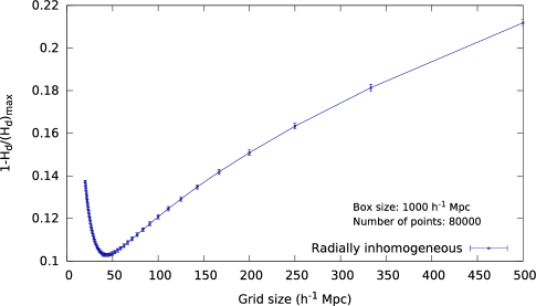
Figure 1: This shows the variation of inhomogeneity $1-\frac{H_{d}}{(H_{d})_{max}}$ as a function of length scales in a radially inhomogeneous Poisson distribution where density falls of as $\frac{1}{r^{2}}$ from one of the corners of a cube with sides $1000\,h^{-1}\,{\rm Mpc}$. The measurements are done using independent and regular cubic voxels as described in section 2. The errorbars shown here are the $1-\sigma$ variations from the $10$ Monte Carlo realizations used.

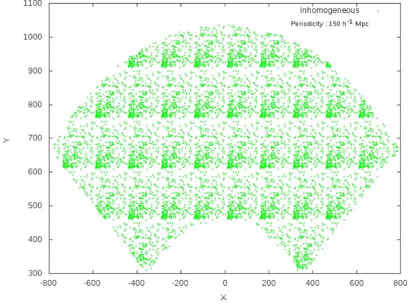
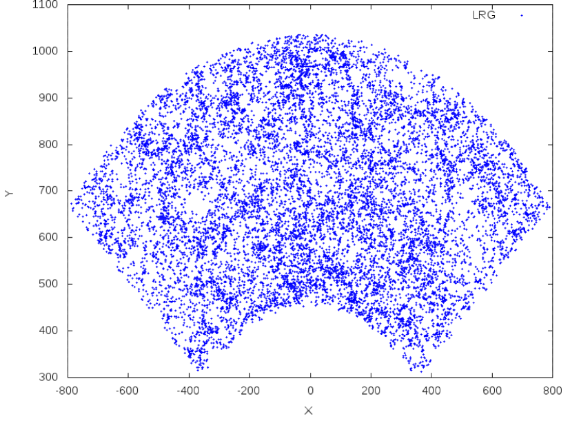
Figure 2: The left panel shows the 2D projected view of an anisotropic and inhomogeneous Poisson distribution which periodically repeats itself at regular intervals of $150\,h^{-1}\,{\rm Mpc}$. The right panel show the projected LRG distribution. Both distributions shown here have an uniform thickness of $200\,h^{-1}\,{\rm Mpc}$. The distributions which are analyzed actually have radially varying thickness.

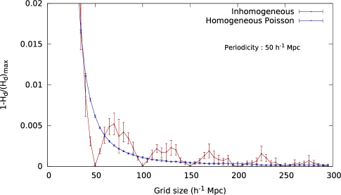
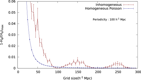
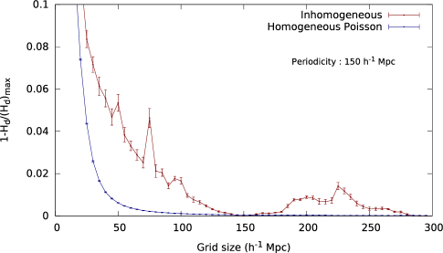
Figure 3: The top left figure shows the inhomogeneity $1-\frac{H_{d}}{(H_{d})_{max}}$ as a function of length scales in an anisotropic and inhomogeneous Poisson distribution which periodically repeats itself at regular intervals of $50\,h^{-1}\,{\rm Mpc}$. The top right and the bottom panels show the same for anisotropic and inhomogeneous Poisson distributions which are periodic on scales of $100\,h^{-1}\,{\rm Mpc}$ and $150\,h^{-1}\,{\rm Mpc}$ respectively. The results shown in all the panels in this figure are obtained using independent and regular cubic voxels as described in section 2. The error-bars shown here in all the panels are the $1-\sigma$ variations from the $10$ Monte Carlo realizations used in each case.

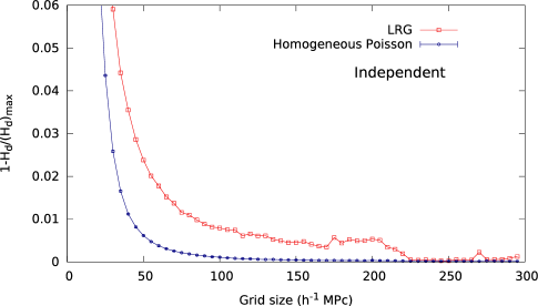
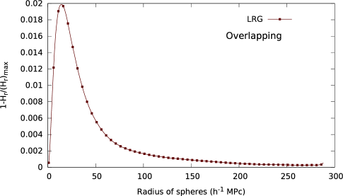
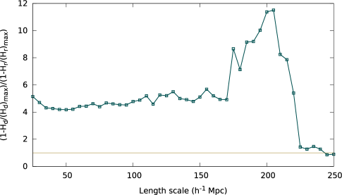
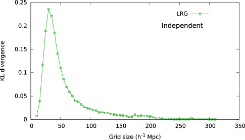
Figure 4: The top left panel shows the inhomogeneity $1-\frac{H_{d}}{(H_{d})_{max}}$ as function of length scales in the LRG distribution and a homogeneous Poisson distribution when the analysis is done with independent voxels as described in section 2. The top right panel shows the inhomogeneity $1-\frac{H_{r}}{(H_{r})_{max}}$ as a function of $r$ in the LRG distribution when the analysis is carried out with overlapping spheres (Pandey, 2013; Pandey et al., 2015). The bottom left panel show the ratio of inhomogeneity on different length scales when measured using independent voxels and overlapping spheres. The bottom right panel show the Kullback-Leibler (KL) divergence measure as a function of length scales when the LRG data is analyzed using independent voxels.

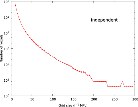
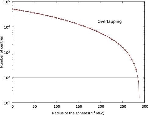
Figure 5: The left panel shows how the number of independent voxels available within the survey region changes with increasing grid sizes. The right panel shows the number of centres available at each radii in the LRG distribution when the analysis is carried out with overlapping spheres.

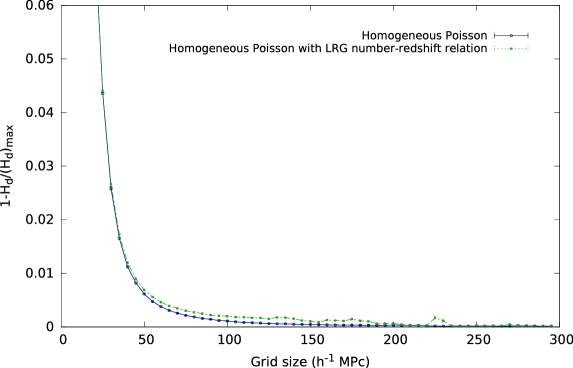
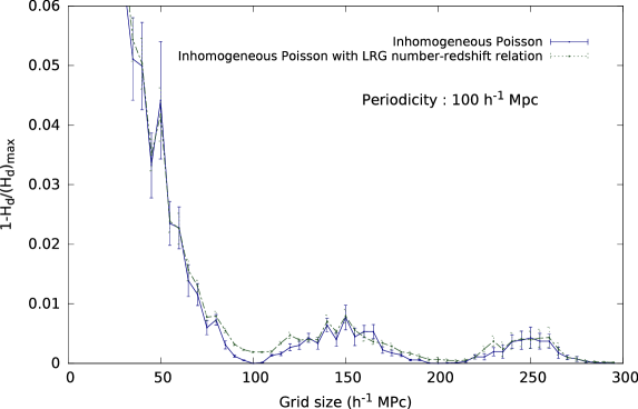
Figure 6: The left panel shows $1-\frac{H_{d}}{(H_{d})_{max}}$ as function of length scales in the mock LRG samples drawn from homogeneous Poisson distributions by enforcing the same comoving number density in them as the actual LRG sample. The results for mock samples without such restrictions are also shown together. The right panels shows the same but for anisotropic and inhomogeneous Poisson distributions which are periodic on scales of $100\,h^{-1}\,{\rm Mpc}$. The error-bars shown here in all the panels are the $1-\sigma$ variations from the $10$ Monte Carlo realizations used in each case.

3 DATA

3.1 LRG DATA

The Sloan Digital Sky Survey (SDSS) (York et al., 2000) is a wide-field imaging and spectroscopic survey of the sky using a dedicated 2.5 m telescope (Gunn et al., 2006) with $3^{\circ}$ field of view at Apache Point Observatory in southern New Mexico. The SDSS has imaged the sky in 5 passbands, $u,\;g,\;r,\;i$ and $z$ covering $10^{4}$ square degrees and has so far made 12 data releases to the community. The SDSS galaxy sample can be roughly divided into two (i) the MAIN galaxy sample and (ii) the Luminous Red Galaxy (LRG) sample. For our work, we have used the spectroscopic sample of LRGs derived from the Data Release 7 of SDSS-II (Abazajian et al., 2009).

SDSS targets those galaxies for spectroscopy which have $r$ magnitude brighter than 17.77 ($r<17.77$). To select LRGs, additional galaxies are targeted using color-magnitude cuts in $g,\;r$ and $i$ which extends the magnitude limit for LRGs to $r<19.5$. The prominent feature for an early-type galaxy is the $4000\,A^{\circ}$ break in its SED. For $z\lesssim 0.4$ this feature lies in the $g$ passband while it shifts to the $r$ band for higher redshifts. Hence selection of LRGs involves different selection criteria below and above $z\lesssim 0.4$, the details of which are described in Eisenstein et al. (2001).

The criteria for lower redshifts are collectively called Cut-I (eq. (4-9) in Eisenstein et al. (2001)) while those for the higher redshifts are called Cut-II (eq. (9-13) in Eisenstein et al. (2001)), with Cut-I accounting for $\approx 80\%$ of the targeted LRGs. A galaxy that passes either of these cuts is flagged for spectroscopy by the SDSS pipeline as TARGET_GALAXY_RED while a galaxy that passes only Cut II is flagged as TARGET_GALAXY_RED_II. Hence, while selecting the LRGs we require that the TARGET_GALAXY_RED and TARGET_GALAXY_RED_II flags both be set.

We obtain the $g$-band absolute magnitude from the $r$ band apparent magnitude accounting for the k-correction and passive evolution. We use the prescription for $K+e$ correction from the Table 1 in Eisenstein et al. (2001) (non-star forming model). The cuts defined above are designed to produce an approximately volume limited sample of LRGs upto $z\approx 0.4$. The comoving number density of LRGs falls sharply beyond $z\approx 0.4$. It is obviously necessary to include LRGs that come from the MAIN sample for $z\lesssim 0.3$. But Eisenstein et al. (2001) issue a strong advisory against selecting LRGs with $z\lesssim 0.15$ for a volume limited sample as the luminosity threshold is not preserved for low redshifts. We have restricted our LRG sample to the redshift range $0.16<z<0.38$ and $g$-band absolute magnitude range $-23<M_{g}<-21$. We identify a region $-50<\lambda<50$ and $-33.5<\eta<29.5$ where $\lambda$ and $\eta$ are the survey coordinates. Combining these cuts provide us our LRG sample which radially extends from $462\,h^{-1}{\rm Mpc}$ to $1037\,h^{-1}{\rm Mpc}$ and consists of $50513$ luminous red galaxies. We have used the same data set in an earlier analysis of filamentarity of LRGs in Pandey et al. (2011). The comoving number density of LRGs as a function of the radial distance $r$ in this sample is shown in Figure 1 of Pandey et al. (2011).

3.2 MONTE CARLO SIMULATIONS

We would like to test if our method can quantify the inhomogeneity and characterize the periodicity in a given spatial distribution. We generate a set of Monte Carlo realizations for an anisotropic distribution with periodicity in their spatial distribution on certain length scale. We decide here to generate the Monte Carlo realizations for a simple radial density distributions $\rho(r)=K\,\lambda(r)$ where $\lambda(r)=\frac{1}{r^{2}}$. Here $K$ is a normalization constant. These distributions are radially inhomogeneous Poisson distributions which are anisotropic at all points other than the centre.

Enforcing the desired number of particles $N$ within radius $R$ one can turn the radial density function into a probability function within $r=0$ to $r=R$ which is normalized to one when integrated over that interval. So the probability of finding a particle at a given radius $r$ is $P(r)=\frac{r^{2}\lambda(r)}{\int_{0}^{R}r^{2}\lambda(r)\,dr}$ which is proportional to the density at that radius implying more particles in high density regions.

We generate the Monte Carlo realizations of this distribution using a Monte Carlo dartboard technique. The value of the function $r^{2}\lambda(r)$ in $P(r)$ is same and constant everywhere. We label the maximum value of $P(r)$ as $P_{max}$ which is same everywhere in this case. We randomly choose a radius $r$ in the range $0\leq r\leq R$ and a probability value is randomly chosen in the range $0\leq P(x)\leq P_{max}$. The actual probability of finding a particle at the selected radius is then calculated using expression for $P(r)$ and compared to the randomly selected probability value. If the random probability is less than the calculated value, the radius is accepted and assigned isotropically selected angular co-ordinates $\theta$ within $0^{\circ}\leq\theta\leq 90^{\circ}$ and $\phi$ within $0^{\circ}\leq\phi\leq 90^{\circ}$, otherwise the radius is discarded. In this way, radii at which particle is more likely to be found will be selected more often because the random probability will be more frequently less than the calculated actual probability. The above $\theta$ and $\phi$ ranges are chosen so as to generate the distribution inside a cubic region. We choose $R=\sqrt{3}L\,h^{-1}\,{\rm Mpc}$ where $L$ is the length of the cube on each side. The value of $N$ is chosen suitably for different $L$ so as to maintain a density which is higher than the mean density of LRGs. We identify all the points whose co-ordinates $(x,y,z)$ lie within $0\leq x\leq L\,h^{-1}\,{\rm Mpc}$, $0\leq y\leq L\,h^{-1}\,{\rm Mpc}$ and $0\leq z\leq L\,h^{-1}\,{\rm Mpc}$. This gives us a cube of side $L\,h^{-1}\,{\rm Mpc}$ containing a certain number of points. We replicate this cube along x,y and z directions as many times as required so as to enable us to extract a region from this periodic distribution which has identical geometry as the LRG distribution. We then randomly select as many points from the extracted region as there are LRGs in our sample.

We choose three different values of $L=50\,h^{-1}\,{\rm Mpc}$, $L=100\,h^{-1}\,{\rm Mpc}$ and $L=150\,h^{-1}\,{\rm Mpc}$ and generate $10$ Monte Carlo realizations of the periodic distributions for each value of $L$. We analyze each set of Monte Carlo realizations separately using the method described in section 2.

A radially inhomogeneous distribution with no preferred scale must appear inhomogeneous on all scales and we want to make sure that the method proposed here efficiently capture the inhomogeneous character of such distribution on all scales. We generate a radially inhomogeneous Poisson distribution in a large cubic box where density falls of as $\frac{1}{r^{2}}$ from one of the corners of the box. The total number of points inside the box is decided so as to maintain a mean density comparable to the mean density of the LRG distribution. $10$ such boxes are generated using the Monte Carlo technique discussed above and analyzed separately using the method presented in section 2.

4 RESULTS AND CONCLUSIONS

We show the inhomogeneity $1-\frac{H_{d}}{(H_{d})_{max}}$ as a function of grid sizes or length scales for the radially inhomogeneous Poisson distributions in Figure 1. The Figure 1 shows that the distribution is inhomogeneous on small scales which is partly due to its inherent inhomogeneous character and partly due to the Poisson noise. The observed inhomogeneity decreases with increasing grid sizes on small scales but suddenly starts increasing at $\sim 50\,h^{-1}\,{\rm Mpc}$ and keep on increasing thereafter. The contribution of Poisson noise to the measured inhomogeneity decreases with increasing grid sizes due to the increase in the number counts inside them and becomes increasingly irrelevant on larger scales. The degree of inhomogeneity on larger scales is primarily decided by the nature of the intrinsic inhomogeneity built in the distribution. We see that for the grid sizes above $50\,h^{-1}\,{\rm Mpc}$ the distribution appears to be increasingly inhomogeneous. This indicates that there is no scale of transition to homogeneity in the distribution and the distribution can be regarded as intrinsically inhomogeneous. It may be noted here that Figure 2 of Pandey (2013) show that the measurement with overlapping spheres leads to suppression in inhomogeneity on large scales which may hide the real inhomogeneous nature of a distribution. The method which employs independent voxels is far more reliable in a sense that there are no artificial reduction in inhomogeneity due to confinement and overlapping biases. It is this advantage which allow us to capture the truly inhomogeneous nature of a distribution as shown in Figure 1. The method presented here is certainly advantageous in this sense and may help us to reliably measure the inhomogeneity present in a distribution on different scales.

In different panels of Figure 3 we show how the inhomogeneities vary with length scales for inhomogeneous and anisotropic distributions which have a periodicity in their spatial distributions (Figure 2). The variations of inhomogeneity in a homogeneous Poisson distribution is also shown together in each panel for comparison. In the top left panel we show the inhomogeneity $1-\frac{H_{d}}{(H_{d})_{max}}$ as a function of grid size for the distributions which are periodic on scales of $50\,h^{-1}\,{\rm Mpc}$. We see that the periodic distributions and homogeneous Poisson distributions both show inhomogeneity on small scales which decrease with increasing length scales. But they vary differently as the degree of inhomogeneity on small scales would depend on the Poisson noise as well as any intrinsic inhomogeneity built in the character of the distributions. It is interesting to note that there is a sharp decrease in the inhomogeneity in the periodic distributions at $50\,h^{-1}\,{\rm Mpc}$. We get $1-\frac{H_{d}}{(H_{d})_{max}}=0$ when the grid size is $50\,h^{-1}\,{\rm Mpc}$ which also is the periodicity of the distributions. The inhomogeneity reappears again as the grid size exceeds $50\,h^{-1}\,{\rm Mpc}$ and decreases once again and disappears exactly at $100\,h^{-1}\,{\rm Mpc}$ and so on. This can be easily explained from the fact that these periodic distributions are highly inhomogeneous below the scale of their periodicity and become homogeneous at the scale at which they are repeated. Once the grid size surpass this scale the distribution would again appear inhomogeneous by partial inclusion of the repeated patterns by the voxels. This behaviour of $1-\frac{H_{d}}{(H_{d})_{max}}$ continues with increasing grid sizes and we get successive minima at repeated intervals of $50\,h^{-1}\,{\rm Mpc}$ showing precise homogeneity on those length scales. The maximum amplitude of the inhomogeneity decreases in successive oscillations due to the decrease in the Poisson noise with increasing grid sizes. The error-bars shown here are the $1-\sigma$ variations from the $10$ Monte Carlo realizations used in each case. The extremely small size of the errorbars on the measured inhomogeneity at each node clearly indicates the presence of a periodicity in the distributions. This characteristic behaviour of inhomogeneity in periodic distributions is markedly different from the smooth decrease of inhomogeneity with increasing length scales in the homogeneous Poisson distributions. We do not find this periodic variation in the homogeneous Poisson distributions as there are no characteristic scales associated with them. The variations of $1-\frac{H_{d}}{(H_{d})_{max}}$ as a function of grid size for periodic distributions with periodicity of $100\,h^{-1}\,{\rm Mpc}$ and $150\,h^{-1}\,{\rm Mpc}$ are shown in the top right and bottom panels respectively. We see similar periodic variations in the measured inhomogeneity at repeated intervals of $100\,h^{-1}\,{\rm Mpc}$ and $150\,h^{-1}\,{\rm Mpc}$ in the respective panels which clearly demonstrate the presence of periodicity in the distributions on those scales. This shows that our method can identify the presence of any regularity in a spatial distribution and quantify the scale over which the patterns are repeated.

We show the inhomogeneity $1-\frac{H_{d}}{(H_{d})_{max}}$ in the LRG distribution and a homogeneous Poisson distribution as a function of length scales in the top left panel of Figure 4 when the data is analyzed with independent voxels. We find that both distributions show inhomogeneity on small scales but the degree of inhomogeneity observed in the LRG distribution is higher than that of a homogeneous Poisson distribution at each length scales. This indicates that the LRGs are not distributed randomly and the amount of information encoded in the LRG distribution is higher as compared to a homogeneous Poisson distribution at each scale. The degree of inhomogeneity in both the LRG and Poisson distribution decrease with increasing length scales but the inhomogeneity in the Poisson distribution decays much faster as compared to the LRG distribution. This can be explained from the fact that the information in the LRG distribution is sourced by the gravitational clustering and Poisson noise whereas for the Poisson distribution the contribution solely comes from the shot noise which becomes increasingly less important on larger length scales. In the top right panel of Figure 4 we show the inhomogeneity $1-\frac{H_{r}}{(H_{r})_{max}}$ in the LRG distribution as a function of length scales when the analysis is carried out with overlapping spheres. We find that the distribution appears to be homogeneous on small scales. The degree of inhomogeneity suddenly rises at a certain length scale after which it gradually decreases with increasing length scales as seen earlier in the top left panel of Figure 4. This characteristic behaviour giving rise to a bump in the inhomogeneity at a given scale arise due to the near uniformity in the distribution on length scale below its mean inter particle separation. It may be noted that the peak of the bump is located at $\sim 23\,h^{-1}\,{\rm Mpc}$ which is the mean intergalactic separation in our LRG sample. A Poisson distribution is expected to become homogeneous on a scale of the average size of voids in the distribution (White, 1979). This is closely related to the mean inter-particle separation and one would expect a Poisson distribution to become homogeneous above this length scale. But we find a large degree of inhomogeneity in the LRG distribution on these length scales. Further we notice that the degree of inhomogeneity in the top right panel is smaller than that in the top left panel at each length scales. These differences are caused by the suppression of inhomogeneities due to confinement and overlapping biases (Pandey, 2013; Kraljic, 2015) which result from the finite volume and progressive overlaps between the measuring spheres with increasing radii. In the bottom left panel of Figure 4 we show the ratio of inhomogeneities measured at different length scales using independent voxels and overlapping spheres. We find that the inhomogeneities are suppressed by a factor of $\sim 5$ upto $170\,h^{-1}\,{\rm Mpc}$ and by a factor of $10$ on even larger scales in the overlapping measurements. The ratio shows a sudden drop at $\sim 200\,h^{-1}\,{\rm Mpc}$ due to the unavailability of sufficient independent voxels beyond this length scale. The results clearly demonstrate the suppression of inhomogeneities on larger length scales when the measuring spheres are allowed to overlap. All the methods for testing homogeneity which are based on the number counts $n(<r)$ in spheres of radius $r$ are equally affected by these biases. Therefore these biases should be properly taken into account in their applications.

In the left panel of Figure 5 we show how the number of available voxels vary with length scales when independent voxels are used for the analysis. Clearly the number of voxels decreases with increasing grid sizes due to the finite volume of the survey region. We see that the number of independent voxels drops below $10$ around $\sim 200\,h^{-1}\,{\rm Mpc}$ and we decide not to consider the scales beyond this in our analysis. The right panel of Figure 5 show the number of available centres as a function of the radius of the spheres when overlapping spheres are used for the analysis. Clearly in this method one can go upto a larger length scales albeit by compromising with larger degree of overlaps between the measuring spheres resulting into a greater degree of suppression in inhomogeneity. We see that one can extend this analysis upto $\sim 270\,h^{-1}\,{\rm Mpc}$ requiring at least $\sim 100$ overlapping spheres. It may be noted in the top right panel of Figure 4 that $1-\frac{H_{r}}{(H_{r})_{max}}$ decreases to $10^{-3}$ at $150\,h^{-1}\,{\rm Mpc}$ and show very little variation thereafter despite the increasing degree of overlaps between the measuring spheres. The value of $1-\frac{H_{d}}{(H_{d})_{max}}$ in the top left panel of Figure 4 also exhibit a quite similar behaviour where its value decreases to $5\times 10^{-3}$ at $150\,h^{-1}\,{\rm Mpc}$ and show a flattening which abruptly drops to $\approx 0$ at $\sim 200h^{-1}\,{\rm Mpc}$. We do not attach any statistical significance to this sudden drop due to the non availability of sufficient number of voxels on that scale. The degree of inhomogeneity at the plateau is somewhat different in the two methods. This difference could be attributed to the fact that inhomogeneities are suppressed by a factor of $\sim 5$ at $150\,h^{-1}\,{\rm Mpc}$ when overlapping spheres are used (Figure 4). We note that $\sim 100$ independent voxels and $>10^{4}$ centers of overlapping spheres are available at $150\,h^{-1}\,{\rm Mpc}$ which trace a very small degree of inhomogeneity present on that scale. The minuscule degree of inhomogeneity measured with a large number of voxels or spheres at the plateau indicates that the LRG distribution is nearly homogeneous on these length scales. The LRG distribution is known to have a linear bias of $\sim 2$ on large scales (Marín, 2011; Sawangwit et al., 2011) and may have a larger variations in $1-\frac{H_{d}}{(H_{d})_{max}}$ as compared to the homogeneous Poisson distributions. Currently we do not have any estimates for the variations in $1-\frac{H_{d}}{(H_{d})_{max}}$ as we have only one distribution for the LRGs. Keeping this in mind we conclude that the LRG distribution becomes homogeneous on scales of $150\,h^{-1}\,{\rm Mpc}$ and beyond. Our results are consistent with the earlier findings that the distribution of galaxies in the SDSS Main sample becomes homogeneous on and above a scale of $140\,h^{-1}\,{\rm Mpc}$ (Pandey et al., 2015). In the bottom right panel of Figure 4 we show the Kullback-Leibler(KL) divergence or the information divergence for the LRG distribution with respect to a homogeneous Poisson distribution on different length scales when the measurements are done with independent voxels. The definition and the significance of this measure is discussed in section 2 and this can be regarded as an alternative measure of inhomogeneity. It is interesting to note that the KL divergence also decreases with increasing grid sizes which is quite similar to the decrease in $1-\frac{H_{d}}{(H_{d})_{max}}$ and $1-\frac{H_{r}}{(H_{r})_{max}}$ with increasing length scales and a similar flattening is observed at $\sim 150\,h^{-1}\,{\rm Mpc}$.

An important caveat to the present analyses arises due the fact that the comoving number density of LRGs varies with redshift and the LRG sample is considered to be only quasi volume limited (Eisenstein et al., 2001; Zehavi et al., 2005; Kazin et al., 2010). These variations could result from both the intrinsic fluctuations in the galaxy density field and the observational selection effects (Sylos Labini, 2010). We test how the presence of such fluctuations in number-redshift relation affect the scale of homogeneity inferred with our method. To test this we construct $10$ mock LRG samples each from homogeneous and inhomogeneous Poisson distributions and randomly exclude points from them so as to finally have the same comoving number density $n(z)$ in them as the actual LRG sample. The results for these analyses are shown in Figure 6. In two panels of Figure 6 we see a small increase in the degree of inhomogeneity when an LRG-like number-redshift relation is enforced in the homogeneous and inhomogeneous Poisson distributions. But we note that the variations of inhomogeneity with length scales in both cases still reflect the characteristics of the underlying distributions and the respective scales of transition to homogeneity in these distributions are not altered by the presence of such a number-redshift relation. However it may be worth mentioning that this test and its outcome rely on a smooth variation in the radial density due to either selection effects or intrinsic fluctuations in the galaxy density field and it is in general difficult to test for any other sources of such fluctuations in the number-redshift relation of LRGs.

We do not see any periodic variation in the measured inhomogeneity $1-\frac{H_{d}}{(H_{d})_{max}}$ of the LRG distribution (Figure 4) in the range of length scales explored. This is in sharp contrast with the variations observed in Figure 3 for periodic distributions. This indicates that there are no underlying regularities in the distribution of the luminous red galaxies at least within the length scales probed in the present work. One can extend this analysis to the LRG sample from the Baryon Oscillation Spectroscopic Survey of SDSS-III (Dawson et al., 2013) and future LRG sample such as from the eBOSS of SDSS-IV (Prakash et al., 2015) to search for any periodic variation in inhomogeneity on even larger scales.

5 ACKNOWLEDGEMENT

The authors would like to thank an anonymous reviewer for useful comments and suggestions. The authors thank Prajwal Raj Kafle for his suggestion for using KL divergence as an alternative measure of inhomogeneity. B.P. would like to acknowledge IUCAA, Pune for providing support through the Associateship Programme. B.P. would also like to acknowledge CTS, IIT Kharagpur for the use of its facilities for the present work.

Funding for the creation and distribution of the SDSS Archive has been provided by the Alfred P. Sloan Foundation, the Participating Institutions, the National Aeronautics and Space Administration, the National Science Foundation, the U.S. Department of Energy, the Japanese Monbukagakusho, and the Max Planck Society. The SDSS Web site is http://www.sdss.org/.

The SDSS is managed by the Astrophysical Research Consortium (ARC) for the Participating Institutions. The Participating Institutions are The University of Chicago, Fermilab, the Institute for Advanced Study, the Japan Participation Group, The Johns Hopkins University, the Korean Scientist Group, Los Alamos National Laboratory, the Max-Planck-Institute for Astronomy (MPIA), the Max-Planck-Institute for Astrophysics (MPA), New Mexico State University, University of Pittsburgh, Princeton University, the United States Naval Observatory, and the University of Washington.

References

- Abazajian et al. (2009) Abazajian, K. N., et al. 2009, ApJS, 182, 543
- Alam et al. (2015) Alam, S., Albareti, F. D., Allende Prieto, C., et al. 2015, arXiv:1501.00963, Accepted to ApJS
- Alonso et al. (2015) Alonso, D., Salvador, A. I., Sánchez, F. J., et al. 2015, MNRAS, 449, 670
- Amendola & Palladino (1999) Amendola, L., & Palladino, E. 1999, ApJ Letters, 514, L1
- Appleby & Shafieloo (2014) Appleby, S., & Shafieloo, A. 2014, JCAP, 10, 070
- Baugh et al. (1998) Baugh, C.M., Cole, S., Frenk, C.S. & Lacey, C.G. 1998, ApJ, 498, 504
- Bengaly et al. (2015) Bengaly, C. A. P., Jr., Bernui, A., & Alcaniz, J. S. 2015, ApJ, 808, 39
- Biswas et al. (2010) Biswas, T., Notari, A., & Valkenburg, W. 2010, JCAP, 11, 30
- Bharadwaj et al. (1999) Bharadwaj, S., Gupta, A. K., & Seshadri, T. R. 1999, A&A, 351, 405
- Bharadwaj et al. (2004) Bharadwaj, S., Bhavsar, S. P., & Sheth, J. V. 2004, ApJ, 606, 25
- Borgani (1995) Borgani, S. 1995, Physics Reports, 251, 1
- Blake & Wall (2002) Blake, C., & Wall, J. 2002, Nature, 416, 150
- Briggs et al. (1996) Briggs, M. S., Paciesas, W. S., Pendleton, G. N., et al. 1996, ApJ, 459, 40
- Broadhurst et al. (1990) Broadhurst, T. J., Ellis, R.S.,Koo, D.C. & Szalay, A.S. 1990, Nature, 343, 726
- Buchert & Ehlers (1997) Buchert, T., & Ehlers, J. 1997, A&A, 320, 1
- Buchert (2001) Buchert, T. 2001, General Relativity and Gravitation, 33, 1381
- Clarkson (2012) Clarkson, C. 2012, Comptes Rendus Physique, 13, 682
- Clifton et al. (2008) Clifton, T., Ferreira, P. G., & Land, K. 2008, Physical Review Letters, 101, 131302
- Coleman & Pietronero (1992) Coleman, P. H., Pietronero, L. 1992, Physics Reports, 213, 311
- Colles et al. (2001) Colles, M. et al.(for 2dFGRS team) 2001,MNRAS,328,1039
- Dai et al. (2013) Dai, L., Jeong, D., Kamionkowski, M., & Chluba, J. 2013, Physical Review D, 87, 123005
- Dawson et al. (2013) Dawson, K. S., Schlegel, D. J., Ahn, C. P., et al. 2013, AJ, 145, 10
- Enqvist (2008) Enqvist, K. 2008, General Relativity and Gravitation, 40, 451
- Eisenstein et al. (2001) Eisenstein, D. J., Annis, J., Gunn, J. E., et al. 2001, AJ, 122, 2267
- Eisenstein et al. (2005) Eisenstein, D. J., Zehavi, I., Hogg, D. W., et al. 2005, ApJ, 633, 560
- Einasto et al. (1997a) Einasto, J., Einasto, M., Gottlöber, S., et al. 1997, Nature, 385, 139
- Einasto et al. (1997b) Einasto, J., Einasto, M., Frisch, P., et al. 1997, MNRAS, 289, 801
- Ellis (2011) Ellis, G. F. R. 2011, Classical and Quantum Gravity, 28, 164001
- Einasto et al. (2015b) Einasto, M., Heinämäki, P., Liivamägi, L. J., et al. 2015, arXiv:1506.05295
- Einasto et al. (2015a) Einasto, M., Gramann, M., Saar, E., et al. 2015, A&A, 580, A69
- Fixsen et al. (1996) Fixsen, D. J., Cheng, E. S., Gales, J. M., et al. 1996, ApJ, 473, 576
- Garcia-Bellido & Haugbølle (2008) Garcia-Bellido, J., & Haugbølle, T. 2008, JCAP, 4, 003
- Gruppuso et al. (2013) Gruppuso, A., Natoli, P., Paci, F., et al. 2013, JCAP, 7, 047
- Gunn et al. (2006) Gunn, J. E., et al. 2006, AJ, 131, 2332
- Gupta & Saini (2010) Gupta, S., & Saini, T. D. 2010, MNRAS, 407, 651
- Guzzo (1997) Guzzo, L. 1997, New Astronomy, 2, 517
- Hanson & Lewis (2009) Hanson, D., & Lewis, A. 2009, Physical Review D, 80, 063004
- Hazra & Shafieloo (2015) Hazra, D. K., & Shafieloo, A. 2015, JCAP, 11, 012
- Hirano & Komiya (2010) Hirano, K., & Komiya, Z. 2010, Physical Review D, 82, 103513
- Hogg et al. (2005) Hogg, D. W., Eisenstein, D. J., Blanton, M. R., Bahcall, N. A., Brinkmann, J., Gunn, J. E., & Schneider, D. P. 2005, ApJ, 624, 54
- Hunt & Sarkar (2010) Hunt, P., & Sarkar, S. 2010, MNRAS, 401, 547
- Huterer et al. (2015) Huterer, D., Shafer, D. L., & Schmidt, F. 2015, arXiv:1509.04708
- Jackson (2012) Jackson, J. C. 2012, MNRAS, 426, 779
- Javanmardi et al. (2015) Javanmardi, B., Porciani, C., Kroupa, P., & Pflamm-Altenburg, J. 2015, ApJ, 810, 47
- Kazin et al. (2010) Kazin, E. A., Blanton, M. R., Scoccimarro, R., et al. 2010, ApJ, 710, 1444
- Kalus et al. (2013) Kalus, B., Schwarz, D. J., Seikel, M., & Wiegand, A. 2013, A&A, 553, A56
- Kashlinsky et al. (2008) Kashlinsky, A., Atrio-Barandela, F., Kocevski, D., & Ebeling, H. 2008, ApJ Letters, 686, L49
- Kashlinsky et al. (2010) Kashlinsky, A., Atrio-Barandela, F., Ebeling, H., Edge, A., & Kocevski, D. 2010, ApJ Letters, 712, L81
- Kolb et al. (2006) Kolb, E. W., Matarrese, S., & Riotto, A. 2006, New Journal of Physics, 8, 322
- Kolb et al. (2010) Kolb, E. W., Marra, V., & Matarrese, S. 2010, General Relativity and Gravitation, 42, 1399
- Kraljic (2015) Kraljic, D. 2015, MNRAS, 451, 3393
- Kurokawa et al. (2001) Kurokawa, T., Morikawa, M., & Mouri, H. 2001, A&A, 370, 358
- Land & Magueijo (2005) Land, K., & Magueijo, J 2005, Phys. Rev. Lett., 95, 071301
- Larena et al. (2009) Larena, J., Alimi, J.-M., Buchert, T., Kunz, M., & Corasaniti, P.-S. 2009, Physical Review D, 79, 083011
- Lin et al. (2015) Lin, H.-N., Wang, S., Chang, Z., & Li, X. 2015, Accepted in MNRAS, arXiv:1504.03428
- Marín (2011) Marín, F. 2011, ApJ, 737, 97
- Martinez & Jones (1990) Martinez, V. J., & Jones, B. J. T. 1990, MNRAS, 242, 517
- Martinez & Coles (1994) Martinez, V. J., & Coles, P. 1994, ApJ, 437, 550
- Martinez et al. (1998) Martinez, V. J., Pons-Borderia, M.-J., Moyeed, R. A., & Graham, M. J. 1998, MNRAS, 298, 1212
- Marinoni et al. (2012) Marinoni, C., Bel, J., & Buzzi, A. 2012, JCAP, 10, 036
- Meegan et al. (1992) Meegan, C. A., Fishman, G. J., Wilson, R. B., et al. 1992, Nature, 355, 143
- Morikawa (1990) Morikawa, M. 1990, ApJ Letters, 362, L37
- Moss et al. (2011) Moss, A., Scott, D., Zibin, J. P., & Battye, R. 2011, Physical Review D, 84, 023014
- Pan & Coles (2000) Pan, J., & Coles, P. 2000, MNRAS, 318, L51
- Pandey & Bharadwaj (2005) Pandey, B., & Bharadwaj, S. 2005, MNRAS, 357, 1068
- Pandey (2010) Pandey, B. 2010, MNRAS, 401, 2687
- Pandey et al. (2011) Pandey, B., Kulkarni, G., Bharadwaj, S., & Souradeep, T. 2011, MNRAS, 411, 332
- Pandey (2013) Pandey, B. 2013, MNRAS, 430, 3376
- Pandey et al. (2015) Pandey, B. & Sarkar, S. 2015, MNRAS, 454, 2647
- Pandey (2015) Pandey, B. 2015, arXiv:1512.03562
- Paranjape (2009) Paranjape, A. 2009, arXiv:0906.3165
- Penzias & Wilson (1965) Penzias, A. A., & Wilson, R. W. 1965, ApJ, 142, 419
- Peebles (1993) Peebles, P. J. E. 1993, Principles of Physical Cosmology. Princeton, N.J., Princeton University Press, 1993
- Planck Collaboration et al. (2014) Planck Collaboration, Ade, P. A. R., Aghanim, N., et al. 2014, A&A, 571, A23
- Prakash et al. (2015) Prakash, A., Licquia, T. C., Newman, J. A., et al. 2015, arXiv:1508.04478
- Ryabinkov et al. (2013) Ryabinkov, A. I., Kaurov, A. A., & Kaminker, A. D. 2013, Ap&SS, 344, 219
- Sarkar et al. (2009) Sarkar, P., Yadav, J., Pandey, B., & Bharadwaj, S. 2009, MNRAS, 399, L128
- Sawangwit et al. (2011) Sawangwit, U., Shanks, T., Abdalla, F. B., et al. 2011, MNRAS, 416, 3033
- Scharf et al. (2000) Scharf, C. A., Jahoda, K., Treyer, M., et al. 2000, ApJ, 544, 49
- Schwarz (2002) Schwarz, D. J. 2002, arXiv:astro-ph/0209584
- Schwarz et al. (2004) Schwarz, D. J., Starkman, G. D., Huterer, D., & Copi, C. J. 2004, Phys. Rev. Lett., 93, 221301
- Schwarz & Weinhorst (2007) Schwarz, D. J., & Weinhorst, B. 2007, A&A, 474, 717
- Scrimgeour et al. (2012) Scrimgeour, M. I., Davis, T., Blake, C., et al. 2012, MNRAS, 3412
- Shannon (1948) Shannon, C. E. 1948, Bell System Technical Journal, 27, 379-423, 623-656
- Skillman et al. (2014) Skillman, S. W., Warren, M. S., Turk, M. J., et al. 2014, arXiv:1407.2600
- Smoot et al. (1992) Smoot, G. F., Bennett, C. L., Kogut, A., et al. 1992, ApJ Letters, 396, L1
- Springel et al. (2005) Springel, V., White, S. D. M., Jenkins, A., et al. 2005, Nature, 435, 629
- Straumann (1974) Straumann, N. 1974, Helvetica Physica Acta, 47, 379
- Sylos Labini et al. (2007) Sylos Labini, F., Vasilyev, N. L., & Baryshev, Y. V. 2007, A&A, 465, 23
- Sylos Labini et al. (2009a) Sylos Labini, F., Vasilyev, N. L., & Baryshev, Y. V. 2009a, Europhysics Letters, 85, 29002
- Sylos Labini et al. (2009b) Sylos Labini, F., Vasilyev, N. L., Pietronero, L., & Baryshev, Y. V. 2009b, Europhysics Letters, 86, 49001
- Sylos Labini (2010) Sylos Labini, F. 2010, arXiv:1011.4855
- Sylos Labini & Baryshev (2010) Sylos Labini, F., & Baryshev, Y. V. 2010, JCAP, 6, 021
- Sylos Labini (2011a) Sylos Labini, F. 2011a, Classical and Quantum Gravity, 28, 164003
- Sylos Labini (2011b) Sylos Labini, F. 2011b, Europhysics Letters, 96, 59001
- Tomita (2001) Tomita, K. 2001, MNRAS, 326, 287
- Valkenburg et al. (2014) Valkenburg, W., Marra, V., & Clarkson, C. 2014, MNRAS, 438, L6
- Watkins et al. (2009) Watkins, R., Feldman, H. A., & Hudson, M. J. 2009, MNRAS, 392, 743
- White (1979) White, S. D. M. 1979, MNRAS, 186, 145
- Wilson & Penzias (1967) Wilson, R. W., & Penzias, A. A. 1967, Science, 156, 1100
- Wu et al. (1999) Wu, K. K. S., Lahav, O., & Rees, M. J. 1999, Nature, 397, 225
- Yadav et al. (2005) Yadav, J., Bharadwaj, S., Pandey, B., & Seshadri, T. R. 2005, MNRAS, 364, 601
- York et al. (2000) York, D. G., et al. 2000, AJ, 120, 1579
- Zehavi et al. (2005) Zehavi, I., Eisenstein, D. J., Nichol, R. C., et al. 2005, ApJ, 621, 22
- Zibin et al. (2008) Zibin, J. P., Moss, A., & Scott, D. 2008, Physical Review Letters, 101, 251303