Abstract

The search for extra dimensions has so far yielded no positive results at the LHC. Along with the discovery of a 125 $\,{\rm GeV}$ Higgs boson, this implies a moderate degree of fine tuning in the parameter space of the Randall-Sundrum model. Within a 6-dimensional warped compactification scenario, with its own interesting phenomenological consequences, the parameters associated with the additional spatial direction can be used to eliminate the need for fine tuning. We examine the constraints on this model due to the 8 $\,{\rm TeV}$ LHC data and survey the parameter space that could be probed at the 14 $\,{\rm TeV}$ run of the LHC. We also identify the region of parameter space that is consistent with the recently reported excess in the diphoton channel in the 13 $\,{\rm TeV}$ data. Finally, as an alternative explanation for the observed excess, we discuss a scenario with brane-localized Einstein-Hilbert terms with Standard Model fields in the bulk.

1 Introduction

The warped geometry model proposed by Randall and Sundrum (RS) [1] is one of the many models in the literature that offer a resolution of the well-known naturalness problem. This model is particularly promising because $(i)$ it resolves the gauge hierarchy problem with large extra dimensions); $(ii)$ the modulus of the extra dimension can be stabilized to a desired value by well-understood mechanisms, e.g. the one due to Goldberger and Wise  [2], and $(iii)$ a similar warped solution can be obtained from a more fundamental theory like string theory where extra dimensions appear naturally [3]. As a result, several search strategies at the LHC were designed specifically [4, 5, 6, 7, 8] to detect signatures of these warped extra dimensions through the decays of Kaluza-Klein (KK) excitations of the graviton which appear at the $\,{\rm TeV}$ scale in this model. The results, so far, have been negative, with the ATLAS Collaboration [9] setting a lower bounds of 2.66 (1.41) $\,{\rm TeV}$ on the mass of the lightest KK excitation of the graviton for a coupling of $k_{5}/\overline{M}_{Pl}$ = 0.1 (0.01). The limits obtained by the CMS Collaboration are similar [5]. This result, together with the very restrictive nature of the RS model, necessitates a fine-tuning of 2-3 orders of magnitude in order to explain the observed Higgs mass of 125 $\,{\rm GeV}$. The model will become even more fine-tuned if the bounds are pushed higher during Run 2 of the LHC.

Some of these difficulties can be eliminated by considering more generalized versions of the RS model. Several such models already exist in the literature [10, 11]. In this work, we focus on one such model which features two extra spatial dimensions with the warping in the two directions being intertwined [12]. The graviton spectrum in this model was worked out in Ref. [13]. While the experiments at the LHC focus entirely on 5-dimensional models, we re-interpret these bounds  [9] and predictions for Run 2  [14], in the context of this multiply warped brane world model.

Interestingly, both the CMS and the ATLAS Collaborations have reported [8, 7] a small excess of events in the $pp\to\gamma\gamma$ channel in the region near $m_{\gamma\gamma}$ = 750 $\,{\rm GeV}$. While this excess can be explained in a whole host of scenarios [15], the CMS collaboration has also attempted a RS-graviton interpretation. However, even with a small value of the effective coupling, namely $k_{5}/\overline{M}_{Pl}$ = 0.01, the ensuing cross-section is much larger than the observed excess. Smaller values of the coupling only occur in an unviable region of parameter space where one must either allow a large hierarchy between the moduli of the extra dimension and the scale of gravity, or, admit greater degrees of fine-tuning in order to resolve the gauge-hierarchy problem. As we shall show, this is not the case with the 6-dimensional scenario where smaller values of the effective coupling arise quite naturally. Based on these considerations, the 6-dimensional model would appear to be a more appealing explanation of the observed signal. However, the statistical significance of the observation is, as yet, too small for any strong claims to be made.

The remainder of this paper is organized as follows : we briefly describe the model in Section 2 and its graviton spectrum in Section 3; the limits on the parameter space are examined in Section 4, the compatibility of the model parameter space and an alternative model that could be in corroboration with the observed diphoton excess are discussed in Section 5; and finally, we conclude in Section 6.

2 6 Dimensions, 4 Branes and Nested Warping

The metric for the 6-dimensional space-time with successive orbifoldings viz. $M^{1,5}\rightarrow[M^{1,3}\times S^{1}/Z_{2}]\times S^{1}/Z_{2}$, is defined as [12]

$$ds^{2}_{6}=b^{2}(z)[a^{2}(y)\eta_{\mu\nu}dx^{\mu}dx^{\nu}+R_{y}^{2}dy^{2}]+r_{z}^{2}dz^{2}\ .$$ (1)

Here, $y,z\in[0,\pi]$ are angular coordinates representing the compactified directions, and $R_{y}$ and $r_{z}$ the respective moduli. Each of the four orbifold fixed points ($y=0$, $z=\pi$, $z=0$ and $z=\pi$) are associated with 4-branes endowed with a localized energy density $V_{i}$. The total gravity action is, thus,

$$\begin{array}[]{rcl}{\cal{S}}=\displaystyle\int d^{4}x\,dy\,dz\sqrt{-g_{6}}\,(M_{6}^{4}R_{6}-\Lambda)&+\displaystyle\int d^{4}x\,dy\,dz\sqrt{-g_{5}}\,[V_{1}(z)\,\delta(y)+V_{2}(z)\,\delta(y-\pi)]\\ &+\displaystyle\int d^{4}x\,dy\,dz\sqrt{-\tilde{g}_{5}}\,[V_{3}(y)\,\delta(z)+V_{4}(y)\,\delta(z-\pi)]\ ,\end{array}$$ (2)

where $M_{6}$ and $\Lambda$ are, respectively, the fundamental scale and the bulk cosmological constant in the 6-dimensional world, whereas $g_{5}$ and $\tilde{g}_{5}$ are the determinants of the induced metrics on the 5-dimensional hypersurfaces.

The solutions to the 6-dimensional Einstein’s equations for negative bulk cosmological constant are given by

$$a(y)=e^{-c|y|}\hskip 42.67912ptb(z)=\displaystyle\frac{\cosh{(kz)}}{\cosh{(k\pi)}}\hskip 42.67912ptc=\displaystyle\frac{R_{y}k}{r_{z}\cosh{k\pi}}\hskip 42.67912ptk=\displaystyle r_{z}\sqrt{\frac{-\Lambda}{10M_{6}^{4}}}\equiv r_{z}\,k^{\prime}\ .$$ (3)

The junctures of the 4-branes constitute 3-branes. Both warp factors $a(y)$ and $b(z)$ are minimized at $(y,z)=(\pi,0)$ and we identify this 3-brane as the one containing the SM. The resulting hierarchy factor is

$$w=e^{-c\pi}\,{\rm sech}(k\pi)\,.$$ (4)

With the natural scale of the Higgs mass being given by $\Lambda_{\rm NP}$, the cutoff scale for the SM, the observed Higgs mass is given by

$$m_{H}\quad=w\,\Lambda_{\rm NP}=w\,\zeta\,{\rm min}(R_{y}^{-1},r_{z}^{-1})\,\,,$$ (5)

where $1\mathrel{\hbox to0.0pt{\raise 2.15277pt\hbox{$<$}\hss}{\lower 2.15277pt\hbox{$\sim$}}}\zeta\mathrel{\hbox to0.0pt{\raise 2.15277pt\hbox{$<$}\hss}{\lower 2.15277pt\hbox{$\sim$}}}10$ parametrizes the uncertainty in $\Lambda_{\rm NP}$, which must be smaller than $M_{6}$. In order to explain a large hierarchy without introducing an unnatural separation of scales between the moduli, Eq.4 along with the relation between $c$ and $k$ in Eq.3 mandates that the warping in one of the two extra dimensions be substantially larger than the other. This can be achieved by having ($i$) a large ($\sim 10$) value for $k$ accompanied by an infinitesimally small $c$, or, ($ii$) a large ($\sim 10$) value for $c$ with a moderately small $k$.

3 The graviton KK modes

The dynamics of the fluctuations about the aforementioned classical metric configuration can be derived within a semi-classical approach [13]. Subsequent imposition of Neumann boundary conditions leads to the quantization of graviton masses. The consequent spectrum is qualitatively different for the two distinct regions of the parameter space, namely, large $k$ and small $k$. In the small $k$ domain, the graviton KK modes, as expected, form nested towers characterised by the winding numbers $n$ and $p$. On the other hand, in the large $k$ domain, the mass difference between successive $n$-levels is so large that only the $n$=0 mode turns out to be relevant in the context of current experiments. The interaction of a graviton with the SM field localized on the 3-brane, is described by

$${\cal L}_{\rm int}=T^{\mu\nu}\Big{(}C_{00}h_{\mu\nu}^{(0,0)}+\sum_{n\neq 0}C_{n0}h_{\mu\nu}^{(n,0)}+\sum_{n,p\neq 0}C_{np}h_{\mu\nu}^{(n,p)}\Big{)}\,$$ (6)

with $T^{\mu\nu}$ being the energy-momentum tensor of the corresponding field. While the detailed results can be found in Ref. [13], we list the important formulae below.

3.1 Mass spectrum and couplings for the KK graviton in large $k$ regime

When $k$ is large and $R_{y}$ & $r_{z}$ have comparable magnitudes, there is little or no warping in the $y$-direction. Hence, to the lowest order, the $y$-momentum eigenstates are just plane waves. This yields $m_{np}^{2}\approx m_{p}^{2}+n^{2}R_{y}^{-2}$, and modes corresponding to $n\neq 0$ are too heavy to be of any consequence to LHC experiments. Effectively, we are left with a single tower of gravitons with masses $m_{0p}\approx m_{p}$. For $p=0$, $m_{p}=0$. For $p\neq 0$, $\nu_{p}=2p+1/2$ and $m_{p}$ is obtained using the relation

$$\begin{array}[]{rcl}\nu_{p}&\equiv&\displaystyle\sqrt{4+\frac{m_{p}^{2}\,R_{y}^{2}}{c^{2}}}\,-\,\frac{1}{2}\ .\end{array}$$ (7)

Up to leading order in $c$, the couplings are given by :

$$C_{00}=\frac{\cosh^{3/2}(k\pi)}{M_{6}^{2}\sqrt{2\pi\,R_{y}\,r_{z}\,B_{0}}}\ ,\qquad C_{0p}=\frac{\cosh^{3/2}(k\pi)}{M_{6}^{2}\sqrt{2\pi\,R_{y}\,r_{z}\,B_{p}}}\,Q_{\nu_{p}}^{5/2}\left(0\right)\ ,$$ (8)

where

$$B_{0}=\int_{-\pi}^{\pi}\cosh^{3}(k\,z)\,dz\ ,\qquad B_{p\,\neq\,0}=\int_{-\pi}^{\pi}{\rm sech}^{2}(k\,z)\left[Q_{\nu_{p}}^{5/2}(\tanh(k\,z))\right]^{2}dz\ .$$ (9)

3.2 Mass spectrum and couplings for the KK graviton in small $k$ regime

Small $k$ implies that the warping in the $z$-direction is small (though not as insignificant as the $y$-warping in the previous case), the mass scale in this direction is substantially high. In other words, $m_{10}\ll m_{01}$. Once again, $\nu_{p}=3/2$ for $p=0$. $m_{np}$ is obtained from

$$m_{np}=\frac{x_{np}c}{e^{-c\pi}R_{y}}\ .$$ (10)

where $x_{np}$ are solutions of

$$\begin{array}[]{rcl}\displaystyle 2x_{np}J_{\nu_{p}-\frac{1}{2}}(x_{np})+(3-2\nu_{p})J_{\nu_{p}+\frac{1}{2}}(x_{np})\,=\,0\ ,\end{array}$$ (11)

$J_{\alpha}$’s being Bessel functions of the first kind (see Ref. [13] for details). The couplings are given by

$$\begin{array}[]{rcl}C_{n0}&=&\displaystyle\frac{e^{c\,\pi}}{M_{6}^{2}r_{z}}\,\cosh(k\,\pi)\,\sqrt{\frac{k}{2\,A_{n0}\,B_{0}}}\,J_{2}(\theta_{\pi})\\[8.61108pt] C_{n,{p\neq 0}}&=&\displaystyle\frac{e^{c\,\pi}}{M_{6}^{2}r_{z}}\,\cosh(k\,\pi)\,\sqrt{\frac{k}{2\,A_{np}\,B_{p}}}\,J_{\nu_{p}+\frac{1}{2}}(\theta_{\pi})\,\left[\cot\theta_{p}\,P_{\nu_{p}}^{5/2}(0)+\,Q_{\nu_{p}}^{5/2}(0)\right]\ ,\end{array}$$ (12)

where $B_{p=0}$ is as before and

$$A_{np}=\int_{0}^{1}r\,\left[J_{\nu_{p}+\frac{1}{2}}(x_{np}\,r)\right]^{2}dr\ ,\qquad B_{p\,\neq\,0}=\int_{-\tau_{\pi}}^{\tau_{\pi}}dr\,\left[\cot\theta_{p}\,P_{\nu_{p}}^{5/2}(r)+\,Q_{\nu_{p}}^{5/2}(r)\right]^{2}\ .$$ (13)

4 Constraining the Parameter Space

In this section we examine the viability of the model described in the previous section in the light of the present LHC data. Furthermore, we confront it with existing projections for Run 2. Before proceeding further, we define two more (dimensionless) quantities :

$$\epsilon\quad\equiv\quad\dfrac{k}{r_{z}M_{6}}\quad=\sqrt{\frac{-\Lambda}{10M_{6}^{6}}}\qquad,\qquad\alpha\quad\equiv\quad\dfrac{R_{y}}{r_{z}}$$ (14)

$\epsilon$ is related to the bulk curvature and the validity of the semi-classical approximations used in extremizing the Einstein-Hilbert action requires $\epsilon<0.1$. Furthermore, we do not expect $R_{y}$ and $r_{z}$ to be vastly different in magnitude since that would lead to a hierarchy in the moduli. Therefore we will only consider $10^{-3}<\alpha<10^{3}$.

In order to perform a systematic scan, we divide the parameter space into the following 4 regions :

• large $k$, large $\alpha$ : $1\leqslant k\leqslant 10$ ; $1\leqslant\alpha\leqslant 10^{3}$

• large $k$, small $\alpha$ : $1\leqslant k\leqslant 10$ ; $10^{-3}\leqslant\alpha<1$

• small $k$, large $\alpha$ : $0.01\leqslant k<1$ ; $1\leqslant\alpha\leqslant 10^{3}$

In each regime, we calculate the mass of the lightest graviton ($m_{01}$ for large $k$ and $m_{10}$ for small $k$), holding $m_{H}=125\,{\rm GeV}$ and restricting $0.0001\leqslant\epsilon\leqslant 0.1$ and $M_{6}<M_{P}$. The ensuing part of the parameter space that supports a KK-graviton within the LHC reach is depicted in Fig.1, and for the remainder of this paper, we consider only these subsets. Note the region small $k$, small $\alpha$ gets completely ruled out as the warping in this domain is not large enough to reproduce the hierarchy between Planck scale and TeV scale.

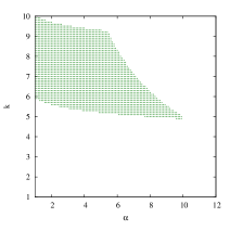
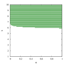
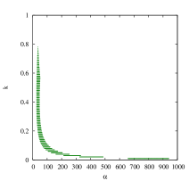
Figure 1: The relevant region of parameter space for $\zeta$ = 1 and (a) large $k$, large $\alpha$, (b) large $k$, small $\alpha$, and (c) small $k$, large $\alpha$. For small $k$, small $\alpha$, the entire region is ruled out by the constraints discussed above.

4.1 Data from the LHC at $\sqrt{s}$ = 8 TeV

Diphoton production is often the preferred channel for gravition searches as it provides a clean signature. The experimental mass resolution in this channel is similar to that for leptons but the branching fraction is larger ($BR(G\to\gamma\gamma)$ = 2 $BR(G\to\ell^{+}\ell^{-})$). The ATLAS Collaboration conducted a search for high invariant mass diphoton pairs resulting from RS graviton decays in the 8 TeV Run of the LHC [9]. They found the data to be consistent with the SM. To interpret the consequent limits in the present context, we must first establish the correspondence between the parameters of the two models. For the RS model, the mass of the lighest KK graviton is given by

$$m_{1}\,=\,m_{G^{*}}\,=\,x_{1}\,k_{5}e^{\pi k_{5}R_{c}}\ ,$$ (15)

where $x_{1}$ is the first root of the Bessel function $J_{1}(x)$. The corresponding graviton interaction term is given by

$$L_{\rm int}^{\rm 5DRS}\quad=\quad\dfrac{k_{5}/\overline{M}_{Pl}}{k_{5}e^{\pi k_{5}R_{c}}}\,\sum_{n=1}^{\infty}T^{\mu\nu}(x)\,h_{\mu\nu}^{(n)}(x)\quad=\quad\dfrac{k_{5}/\overline{M}_{Pl}}{m_{G^{*}}/x_{1}}\,\sum_{n=1}^{\infty}T^{\mu\nu}(x)\,h_{\mu\nu}^{(n)}(x)\ .$$ (16)

Comparing Eq.16 with Eq.6, it is only natural to bridge the 5-dimensional and 6-dimensional models with

$$\dfrac{k_{5}/\overline{M}_{Pl}}{m_{G^{*}}/x_{1}}\longleftrightarrow|C_{01}|,\,|C_{10}|\ ,\qquad m_{G^{*}}\longleftrightarrow|m_{01}|,\,|m_{10}|\ .$$ (17)

as they form equivalent descriptions for the collider analysis. With this mapping in place, the remainder of the analysis follows exactly as that for the 5-dimensional RS model. For a graviton of a given mass and a given final state (diphoton in this case), the phase-space distribution of the final state particles is identical for the two models. Accordingly, detector resolution, efficiency of cuts and overall experimental sensitivity would also be practically identical. On the theoretical front, QCD and electroweak NLO corrections too would be identical to those for the RS model (see Footnote 1). Hence one can directly identify the ATLAS limits on the $k_{5}/\overline{M}_{Pl}-m_{G^{*}}$ plane onto the $C_{01}-m_{01}$ ($C_{10}-m_{10}$) plane for the large $k$ (small $k$) case.

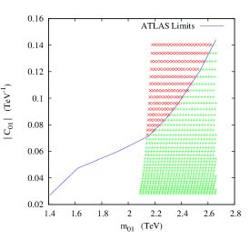
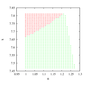
Figure 2: The red $\times$’s (green $+$’s) show the parts of large $k$, large $\alpha$ parameter space (for $\zeta$ = 1) ruled out (allowed) by the ATLAS[9] limits (blue curve). All the points depicted satisfy the initial requirements on $\epsilon$ and $M_{6}$.

Fig.2(a) shows the limits on the $C_{01}-m_{01}$ plane for the large $k$, large $\alpha$ scenario. Since the limits are based on 8 $\,{\rm TeV}$ data, the sensitivity to KK graviton masses extends only upto 2.5 $-$ 3 $\,{\rm TeV}$. The $\times$’s above the curve are show the region that is ruled out. The corresponding region in the $k-\alpha$ plane is shown in Fig.2(b). Once again $\times$’s denote the region that is ruled out.

A similar exercise can be carried out for the large $k$, small $\alpha$ case. The results are depicted in Fig.3. On the other hand, the small $k$, large $\alpha$ region remains unconstrained by the 8 TeV LHC data as the values of $m_{10}$ are typically larger than 3 TeV in this case.

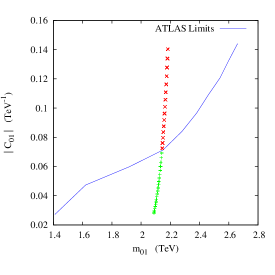
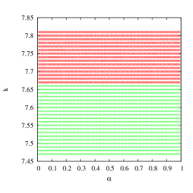
Figure 3: As in Fig.2, but for the large $k$, small $\alpha$ regime instead.

4.2 14 TeV Projections

In Ref. [14], the authors used Monte Carlo simulations at NLO along with parton showers, and obtained projections for the lower limits on $m_{G^{*}}$ that may be extracted from the $\ell^{+}\ell^{-}$ (Drell-Yan) and $\gamma\gamma$ (Diphoton) final states with an integrated luminosity of 50 fb^-1 for certain benchmark values of $k_{5}/\overline{M}_{Pl}$. The results are presented in Table 1 and Table 2, respectively, of Ref. [14].

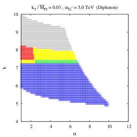
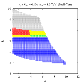
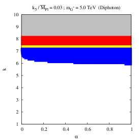
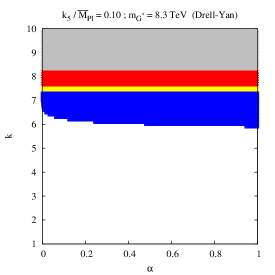
Figure 4: Exclusion of parameter space based on limits from Ref.[14]. Upper row $-$ large $k$, large $\alpha$; lower row $-$ large $k$ small $\alpha$. $\zeta$ = 1. See text for detailed description.

We now examine what these limits signify for the surviving parameter space of the 6-dimensional model as depicted by Fig.1. At the outset, we note that if the coupling is very large, it can lead to the graviton’s width being larger than its mass. Such couplings are clearly unphysical as they would invalidate any particle description for gravitons. The region of in the $k$-$\alpha$ plane that leads to such large, unphysical couplings is marked by grey triangles in Fig. 4. The limits obtained in Ref. [14] are based on an integrated luminosity of 50 fb^-1. The LHC is expected to accumulate about 3000 fb^-1 in its lifetime [16]). For a given mass, the sensitivity to $C_{np}$ obtained from the above analysis would then be extended to $(50/3000)^{1/4}C_{np}\approx 0.36C_{np}$. Values of $C_{np}$ smaller than this would not be probed by the LHC. The corresponding part of the $k$-$\alpha$ plane is marked by blue boxes in Fig. 4.

For $k_{5}/\overline{M}_{Pl}$ = 0.03, Ref. [14] finds the lower limit on $m_{G^{*}}$ to be 5.0 TeV. This implies that for $C_{np}\geqslant$ 0.023, $m_{np}\leqslant$ 5.0 TeV would be ruled out. In Fig. 4, this region is denoted in by red $\times$’s. The complementary region, with smaller couplings and larger masses is allowed and shown by green $+$’s. For smaller masses and couplings, the resonance may be observed with a lower significance, whereas if both the coupling and the mass are larger, the signal would take the form of a deviation in the tail of the invariant mass spectrum. Such regions are denoted, respectively, by lower-left and upper-right regions marked by yellow stars in Fig. 4(a) & (b) [large $k$, large $\alpha$]. In Fig. 4(c) & (d) [large $k$, small $\alpha$], the entire yellow region corresponds to smaller masses and couplings. The small $k$, large $\alpha$ region leads to couplings that are too small to be probed by the LHC. Hence the entire region in Fig 1(c) would survive the LHC.

5 The excess at $m_{\gamma\gamma}$ = 750 GeV

Recently, both the ATLAS [7] and CMS [8] collaborations have reported an excess in the diphoton mass spectrum near $m_{\gamma\gamma}\sim$ 750 $\,{\rm GeV}$. A spin-1 resonance interpretation for this excess is ruled out due to considerations of angular momentum conservation and the fact that the final state consists of identical particles. The ATLAS collaboration has analyzed the excess in the context of a Higgs-like (spin-0) particle. The CMS analysis has considered the RS-graviton interpretation and found the excess to be most compatible with $m_{G*}$ = 760 GeV for an effective coupling $k_{5}/\overline{M}_{Pl}$ = 0.01. In a later update [17], the ATLAS collaboration has presented a spin-2 analysis in which they find that the largest deviation from the background-only hypothesis occurs for signal hypothesis corresponding to $k_{5}/\overline{M}_{Pl}$ = 0.21 and $m_{G*}$ = 750 GeV.

The existence of an excess in the 13 $\,{\rm TeV}$ data, when viewed in the context of lack of any such excess in the 8 $\,{\rm TeV}$ data points to gluon-gluon fusion as the dominant production mechanism. While many models have been proposed, most have sought to explain the excess in terms of a $J=0$ state. The CMS analysis for the 5-dimensional RS scenario suggests that the observed rates are too low even for $k_{5}/\overline{M}_{Pl}=0.01$, a value already at the edge of the aesthetically acceptable region for $k_{5}/\overline{M}_{Pl}$. Indeed, this was to be expected given the existing studies of RS gravitons. Furthermore, with RS gravitons coupling universally to the SM fields, such a diphoton excess, would, be accompanied by similar excesses in other channels (most notably in $e^{+}e^{-},\mu^{+}\mu^{-},W^{+}W^{-},ZZ,t\bar{t}$ and $hh$), none of which have been seen.

As we have learned in the preceding section, the situation is markedly different for 6-dimensional nested warping, on account of both the change in the spectrum as well as the coupling of the graviton to th SM fields. This opens up the possibility of a signal strength commensurate with the observed excess. We now examine this in detail. The issue of the lack of excess in other channels remains and we will return to it at a later stage.

In the preceding sections, we have restricted ourselves to the case where $\zeta$ = 1, i.e. where $\Lambda_{\rm NP}$ for the SM is identified with $min(R_{y}^{-1},r_{z}^{-1})$. However, in order to have $m_{np}\in[700,800]$ $\,{\rm GeV}$ along with suitable couplings, we need to allow $\zeta>1$ and moderately large $\alpha$. In the case of small $k$, large $\alpha$, the requirement $\epsilon<$ 0.1 causes the typical values $C_{np}$ to be lower than the equivalent 5-dimensional RS coupling. As a result the graviton production cross-section in the 6-dimensional model would be lower than that in the 5-dimensional model, and, in fact, is likely to be more compatible with the observed excess. For the choice $\zeta$=7, we plot this favoured sector of the parameter space in Fig.5 in (a) the $m_{10}-|C_{10}|$ plane, and (b) the $m_{10}-k_{5}/\overline{M}_{Pl}$ plane. The relation between $k_{5}/\overline{M}_{Pl}$ and $C_{10}$ was noted earlier in Eq.17. Fig.5(c) shows the same region in the $k-\alpha$ plane. Note that the value of $\zeta$ is chosen for illustrative purposes. While it is indicative of the likely order of magnitude of the quantity, it is not a special or critical or ’best-fit’ value.

Turning to the large $k$, large $\alpha$ case, we find that there exist sectors in the parameter space where $m_{01}\in$ [700, 800] $\,{\rm GeV}$ and $C_{01}$ lies in the region close to $k_{5}/\overline{M}_{Pl}=0.01$. In Fig.6 we plot this sector of parameter space in the $m_{01}-|C_{01}|$, $m_{01}-k_{5}/\overline{M}_{Pl}$ and the $k-\alpha$ planes. This time we assume $\zeta$=10.

Clearly these regions of parameter space are neither fine-tuned nor do they involve large hierarchies between $R_{y}$ and $r_{z}$. In fact, they provide a rather satisfactory explanation for the observed deviation from the SM. Should the observation of a resonance be confirmed with more data, further exploration of this region of parameter space would be in order.

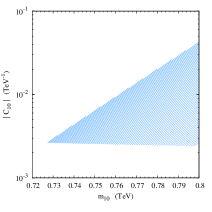
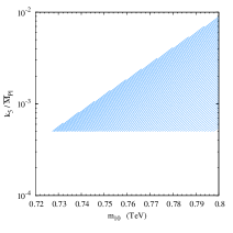
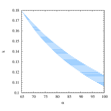
Figure 5: The region of parameter space, for small $k$, large $\alpha$ regime with $\Lambda_{\rm NP}=7R_{y}^{-1}$, consistent with the recently reported excess in the diphoton invariant mass spectrum in the 13 TeV run of the LHC [7, 8].

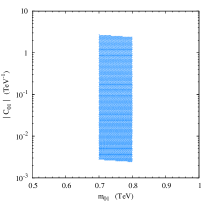
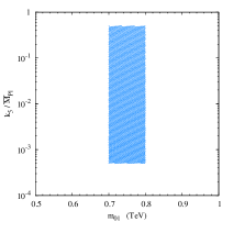
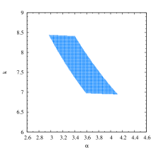
Figure 6: As in Fig.5, but for large $k$, large $\alpha$ and $\Lambda_{\rm NP}=10R_{y}^{-1}$.

5.1 Corroborative signals from other channels

We now return to the postponed question of the lack of signals in other channels. Since gravitons have a universal coupling to all brane-localized SM particles, one would expect that the excess in the diphoton channel would be accompanied by excesses corresponding to the same invariant mass in the dilepton, dijet, $WW$ and $ZZ$ channels. However, none such have been reported as yet. In their updated results on the diphoton channel, the ATLAS collaboration reports [17] an excess of 25 events in the invariant mass range 700 - 840 GeV. Assuming that this accurately represents the expectations from a graviton excitation (in a theory where all the SM fields are localized on the IR-brane), this would translate to   390 additional events in the diject channel,  12 additional events in each of the dielectron and dimuon channel,  42 additional events in the WW-channel and  21 additional events in the ZZ channels ( for the last two, all decay modes of the gauge boson have been summed over). It should be realized though that these numbers are only indicative (derived as they are with kinematic restrictions identical to those enforced in the diphoton channel) and would change when the actual analysis cuts are imposed instead. We now discuss each of them in turn.

• Dijet [18, 19]: While the analyses focus on $m_{jj}>1.1$ $\,{\rm TeV}$, it can be seen that for $m_{jj}\in[700,800]$ $\,{\rm GeV}$, the SM expectation is in excess fo $10^{5}$ events. An excess of 390 events would correspond to a small significance ($S/\sqrt{B}<1$).

• $WW$ and $ZZ$ [20, 21]: The searches conducted by ATLAS are in modes where at least one of the $W$’s or $Z$’s decays into leptons, leading to a further suppression of the signal due to the small branching ratio of $W$ and $Z$ into leptons. Consequently, the lack of the signal so far is only to be expected. And while CMS does consider hadronic decays of the W and Z, they have, yet, considered only invariant mass above 1 $\,{\rm TeV}$. Given the fact the SM background are larger for lower invariant masses, it requires more statistics to resolve the excess in this channel. This situation is in marked contrast with the case of a spin-0 resonance, where, for the simplest models, decay into the diphoton channel tends to be significantly suppressed with respect to the decay into $W^{+}W^{-}$ and $ZZ$

• Dilepton [22, 23]: In the dielectron channel, the background expectation is approximately 53 events. An additional 12 events coming from a graviton decay would only result in low signal significance with $S/\sqrt{B}\sim$ 1.6. A similar argument holds for dimuon production.

In other words, the absence of excesses in the dijet, WW, ZZ dilepton channels is not yet really worrisome at least, at present. It might be argued though that while the individual negative results are not bothersome, in totality they present a strong counterargument to the hypothesis of a 750 $\,{\rm GeV}$ graviton with the 6-dimensional nested warping. Indeed if additional data continues to project the same features as the current one, the simple model that presented here would be under threat and a suitable mechanism should be formulated. We turn to this now.

5.2 An alternative scenario

The primary problem with the graviton interpretation for an excess confined to a single channel arises from the fact that the branching fractions of a universally coupling graviton are uniquely determined. Deviations from universality are possible, though, if the fermions and gauge bosons have different wave profiles in the extra-dimensions. This can be achieved by a minimal extension allowing SM particles to propagate into the bulk.

While such an extension into the entire bulk has been considered in Ref. [31], we restrict ourselves to a simpler scenario wherein the SM fields are five-dimensional entities rather than full six-dimensional ones. Apart from offering the simplest extension that solves the problem at hand, the construction presented below is a novel one. There are two special locations where the SM 4-brane could exist, namely as a hypersurface at $z=0$ or one at $y=\pi$. The choice depends on the extent of warping associated with the two directions which, in turn, play a pivotal role in defining the wavefunction and the consequent hierarchy in the fermion masses on the one hand and the coupling to the putative 750 $\,{\rm GeV}$ graviton on the other. We choose $z=0$ and $y=\pi$ branes for small $k$ and large $k$ respectively. It should also be appreciated that, with the SM fields now being five-dimensional, $\zeta>1$ is natural.

It is well known that, in the case of a five-dimensional Standard model in a Randall-Sundrum background, the zero mode of light fermions (heavy fermions) are localized dynamically near the UV (IR) 3-brane, with the degree of localization controlled by the bulk Dirac mass term [24, 25, 26]. This serves to explain the fermion mass hierarchy. On the other hand, the gauge boson zero modes have a flat profile in the extra-dimension. This difference between gauge bosons and fermions along with the fact that KK gravitons, (except the zero-mode graviton) are localized near the IR brane can engender a suppression in the graviton decay width to dileptons in comparison with the decay to diphotons.

As in previous sections, we are posed with two distinct regimes, namely, large $k$ and the other small $k$. Having large $k$, along with bulk SM fields, leads to large, non-perturbative gauge boson-fermion couplings which is phenomenologically disfavoured [31]. Hence we concentrate on the small $k$ scenario, with the SM particles propagating on the 4-brane located at $z=0$ with the line element given by

$$ds_{5}^{2}=e^{-2c\,|y|}\eta_{\mu\nu}dx^{\mu}dx^{\nu}+R_{y}^{2}dy^{2}\,.$$

The gauge fields can be decomposed into KK-towers of 4-dimensional fields, with the $y-$dependent factor int he wavefunction being given in terms of

$$\Psi_{v}^{(n)}(y)=\frac{1}{N_{n}}e^{cy}\Big{(}J_{1}(\frac{m_{n}R_{y}}{c}e^{cy})+\beta_{n}Y_{1}(\frac{m_{n}R_{y}}{c}e^{cy})\Big{)}$$

In particular, the zero-mode ( to be identified with the SM field) have a simpler form

$$\Psi_{v}^{(0)}(y)=\frac{1}{\sqrt{\pi}}$$

and, consequently, the coupling of the graviton to a pair of vector bosons ( W, Z) remains unchanged.

As for the fermions, the very fact of them being vector like allows bulk mass terms viz, $m_{D}\bar{\psi_{D}}\psi_{D}+m_{S}\bar{\psi_{S}}\psi_{S}$ where $\psi_{D}$ and $\psi_{S}$ refers to $SU(2)_{L}$ doublets and singlets respectively, apart from the brane localized terms occurring from spontaneous symmetry breaking. Neglecting the latter ( on account of them being much smaller than $m_{D}$ or $m_{S}$, the natural scale for these being $R_{y}^{-1}$), the wavefunction for the zero-mode can be seen to be

$$\Psi_{f}(y)=\sqrt{c\frac{1-2\tilde{m}}{e^{(1-2\tilde{m})c\pi}-1}}e^{(2-\tilde{m})cy}$$

where $\tilde{m}=mr_{c}/c$ with $m=m_{D},m_{S}$ as the case may be. Once again the calculation of the graviton coupling is straight forward. In Fig. 7 we display the ratio of the graviton’s coupling to fermions ($g_{f}$) to that with gauge bosons ($g_{v}$); asserting $m_{D}$ and $m_{S}$ to be equal and independent of fermion’s identity. and it can be seen that it is not difficult to obtain a suppression large enough to evade the constraints from the dilepton decay channel. Indeed, with small variations in $m_{D},m_{S}$, differing fermionic branching ratios can be easily accommodated were such a thing to be demanded by future measurements.

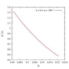
Figure 7: The ratio of the coupling of the first graviton KK-mode to fermions ($g_{f}$) and gauge bosons ($g_{v}$).

It should be noted that with the Standard Model fields being in the 5-dimensional bulk, the requirements of custodial symmetry and consistency with electroweak precision measurements mean that the first KK gauge boson mass has to be greater than $3$   TeV. This leads us into trouble, since the mass of the first KK graviton mode has to be greater than the first KK gauge boson mass by a factor $1.59$, and it debars the graviton from acquiring a mass of 750 GeV. The resolution to this conundrum is to incorporate 4-brane localized Einstein-Hilbert action [28, 29]. For small $k$ we choose to localize the five-dimensional Einstein-Hilbert term on $y=0$ and $y=\pi$ 4-branes. The total action including the brane localized terms is

$$S_{g}=M_{6}^{4}\int d^{4}x\int dy\int dz\Big{(}\sqrt{-g}R^{(6)}+\sqrt{-g_{5}}\,R_{y}\,\{\,g_{0}\,\delta(y)\,+\,g_{\pi}\,\delta(y-\pi)\,\}R^{(5)}\Big{)}\,,$$

where $\sqrt{-g}=a^{4}b^{5}R_{y}r_{z}$ and $\sqrt{-g_{5}}=a^{4}b^{4}r_{z}$. $g_{0}$ and $g_{\pi}$ are numerical coefficients that denote the strengths of the brane localized kinetic terms. The origin of such brane could be quantum mechanical in nature [27], and here we choose to work with the lowest order in $R$, as this will be dominant contributor.

The relevant part of the action, since we are interested only in the spectrum of $h_{\mu\nu}$, could be written as

$$S_{g}=M_{6}^{4}\int d^{4}x\int dy\int dz\Big{(}\sqrt{-g}\,\partial^{M}h_{\mu\nu}\,\partial_{M}h_{\mu\nu}+\sqrt{-g_{5}}\,R_{y}\,\{\,g_{0}\,\delta(y)\,+\,g_{\pi}\,\delta(y-\pi)\,\}\partial^{\bar{M}}h_{\mu\nu}\partial_{\bar{M}}\,h_{\mu\nu}\Big{)}\,$$

with $M=(0,1,2,3,4,5)$ and $\bar{M}=(0,1,2,3,5)$

With $g_{0}$ and $g_{\pi}$ proportional to $b(z)$, the modified graviton masses are, as derived in  [28], given by

$$\xi_{1}(\alpha_{10})-\frac{1}{2}g_{\pi}\,c\,\alpha_{10}\,\xi_{2}(\alpha_{10})=0\,,$$ (18)

where $\alpha_{10}=\frac{m_{10}R_{y}}{c}e^{c\pi}$ and

$$\xi_{q}=J_{q}(\alpha_{10}\,e^{c(|y|-\pi)})+\beta_{10}\,Y_{q}(\alpha_{10}\,e^{c(|y|-\pi)})\,,\quad(q=1,2)$$

with $\beta_{10}$ given as

$$\beta_{10}=-\frac{J_{1}(\alpha_{10}e^{-c\pi})+g_{0}\frac{cR_{y}}{2}\alpha_{10}e^{-c\pi}J_{2}(\alpha_{10}e^{-c\pi})}{Y_{1}(\alpha_{10}e^{-c\pi})+g_{0}\frac{cR_{y}}{2}\alpha_{10}e^{-c\pi}Y_{2}(\alpha_{10}e^{-c\pi})}\,.$$

Note that for $m_{10}$ of the order $\,{\rm TeV}$, the constant of integration $\beta_{10}\ll 1$, and hence in Eq. 18 we could safely ignore the contribution from Bessel Y function. The mass spectrum is independent of $g_{0}$, and with small $g_{\pi}$, the spectrum tends to the root of $J_{1}$ as expected. Using the relation in Eq. 18 the modified mass for the first KK mode of graviton could be calculated for different values of $\frac{1}{2}cg_{\pi}$. This is plotted in Fig. 8, where it is easy to see that for a suitable value of $k$ we do not need a large $g_{\pi}$ to achieve $750\,{\rm GeV}$ graviton mass. Moreover, the constraint on the mass of the first KK mode of gauge bosons from electroweak precision data is satisfied.

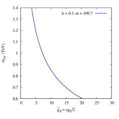
Figure 8: Variation in the mass of the first KK-mode graviton with respect to $\frac{1}{2}cg_{\pi}$, for $k=0.1$ and $\alpha=109.7$ keeping $\epsilon=0.1$. The mass of the first KK-mode of the gauge boson is held at $M_{A}\sim 3\,{\rm TeV}$. For $m_{10}$ = 0.75 TeV, $\frac{1}{2}cg_{0}$ = 40, $\frac{1}{2}cg_{\pi}$ = 13 and $|C_{10}|=3\times 10^{-3}\,{\rm TeV}^{-1}$.

6 Discussion and Summary

The search for extra dimensions by ATLAS and CMS along with the discovery of a 125 $\,{\rm GeV}$ Higgs boson at the LHC have diminished the parameter space of the 5-dimensional Randal-Sundrum model. An alternative minimal extension of the Randall-Sundrum model was proposed in Ref. [12] which allowed for a light Higgs inspite of the gravitons being considerably heavy. This was achieved by admitting a doubly warped 6-dimensional manifold with four 4-branes protecting the edges at the orbifold fixed points. The existence of fifth spatial dimension introduces some extra parameters (though not all independent) in the form of modulus hierarchy and warp factors. In this paper we have identified the regions in the parameter space of this model that survive the current LHC constraints and those that can tested during Run 2 of LHC.

We have examined three regimes, namely large $k$ large $\alpha$, large $k$ small $\alpha$ and small $k$ large $\alpha$. The latter is unconstrained by present LHC data since the KK gravitons in the parameter space are heavier than the energy scale probed by 8 $\,{\rm TeV}$ LHC. But the large $k$ scenario gets constrained and this is shown in Fig.2 and Fig.3

$k>$ 8 is disfavoured as they lead the graviton’s width to be larger than its mass whereas $k<$ 0.8 is inaccessible at the LHC. Other than this, comparison with predictions for the Drell-Yan and diphoton processes at 14 $\,{\rm TeV}$ with 50 fb^-1 worth of data [14] seem to imply that a wide range of $\alpha$ values can be accommodated across the two $k$ regimes.

Finally we have delineated the region of parameter space that can explain the reported excess in the $m_{\gamma\gamma}$ distribution measured in the 13 $\,{\rm TeV}$ run of the LHC. The significance of the excess is, at present, rather small. However, in case this significance increases with accumulation of more data, the 6-dimensional multiply warped model discussed here would certainly make for a compelling explanation for, on the one hand the model has several interesting features, and, on the other, a 750 GeV graviton comes about quite naturally without stretching the parameter space. We have also outlined a possible mechanism that would naturally give rise to a low mass graviton with dilepton couplings being suppressed in comparison to diphoton couplings. In case, even after the accumulation of more data, no excess is seen in the dilepton channel, this scenario will assume greater importance.

References

- [1] L. Randall and R. Sundrum, Phys. Rev. Lett. 83, 3370 (1999); ibid 83, 4690 (1999).
- [2] W.D. Goldberger and M. B. Wise, Phys. Rev. Lett. 83, 4922 (1999).
- [3] M.B. Green, J.H. Schwarz and E. Witten, “Superstring Theory”,Vols.I & II, Cambridge University Press (1987); J. Polchinski, “String Theory”, Cambridge University Press (1998).
- [4] G. Aad et al. [ATLAS Collaboration], New J. Phys. 15 (2013) 043007; arXiv:1506.00962 [hep-ex].
- [5] The CMS Collaboration, CMS-PAS-EXO-12-045.
- [6] G. Aad et al. [ATLAS Collaboration], Phys. Rev. D 90 (2014) 5, 052005; V. Khachatryan et al. [CMS Collaboration], JHEP 1504 (2015) 025; JHEP 1408 (2014) 174.
- [7] The ATLAS Collaboration, ATLAS-CONF-2015-081.
- [8] The CMS Collaboration, CMS-PAS-EXO-15-004.
- [9] G. Aad et al. [ATLAS Collaboration], Phys. Rev. D 92, 032004 (2015).
- [10] M. Gogberashvili and D. Singleton, Phys. Lett. B 582, 95 (2004); Phys. Rev. D 69, 026004 (2004); M. Gogberashvili, P. Midodashvili and D. Singleton, JHEP 0708, 033 (2007).
- [11] S. L. Parameswaran, S. Randjbar-Daemi and A. Salvio, Nucl. Phys. B 767, 54 (2007); A. Salvio, Phys. Lett. B 681, 166 (2009).
- [12] D. Choudhury and S. SenGupta, Phys. Rev. D 76, 064030 (2007).
- [13] M. T. Arun, D. Choudhury, A. Das and S. SenGupta, Phys. Lett. B 746, 266 (2015).
- [14] G. Das, P. Mathews, V. Ravindran and S. Seth, JHEP 1410, 188 (2014).
- [15] W. Chao, arXiv:1512.06297 [hep-ph]; J. Bernon and C. Smith, arXiv:1512.06113 [hep-ph]; L. M. Carpenter et al. arXiv:1512.06107 [hep-ph]; E. Megias et al. arXiv:1512.06106 [hep-ph]; A. Alves et al. arXiv:1512.06091 [hep-ph]; J. S. Kim et al. arXiv:1512.06083 [hep-ph]; S. Ghosh et al. arXiv:1512.05786 [hep-ph]; Y. Bai et al. arXiv:1512.05779 [hep-ph]; A. Falkowski et al. arXiv:1512.05777 [hep-ph]; C. Csaki et al. arXiv:1512.05776 [hep-ph]; P. Agrawal et al. arXiv:1512.05775 [hep-ph]; A. Ahmed et al. arXiv:1512.05771 [hep-ph]; J. Chakrabortty et al. arXiv:1512.05767 [hep-ph]; L. Bian et al. arXiv:1512.05759 [hep-ph]; D. Curtin and C. B. Verhaaren, arXiv:1512.05753 [hep-ph]; S. Fichet et al. arXiv:1512.05751 [hep-ph]; W. Chao et al. arXiv:1512.05738 [hep-ph]; S. V. Demidov and D. S. Gorbunov, arXiv:1512.05723 [hep-ph]; J. M. No et al. arXiv:1512.05700 [hep-ph]; D. Becirevic et al. arXiv:1512.05623 [hep-ph]; P. Cox et al. arXiv:1512.05618 [hep-ph]; A. Kobakhidze et al. arXiv:1512.05585 [hep-ph]; S. Matsuzaki and K. Yamawaki, arXiv:1512.05564 [hep-ph]; Q. H. Cao et al. arXiv:1512.05542 [hep-ph]; B. Dutta et al. arXiv:1512.05439 [hep-ph]; E. Molinaro et al. arXiv:1512.05334 [hep-ph]; C. Petersson and R. Torre, arXiv:1512.05333 [hep-ph]; R. S. Gupta et al. arXiv:1512.05332 [hep-ph]; B. Bellazzini et al. arXiv:1512.05330 [hep-ph]; M. Low et al. arXiv:1512.05328 [hep-ph]; J. Ellis et al. arXiv:1512.05327 [hep-ph]; S. D. McDermott et al. arXiv:1512.05326 [hep-ph]; S. Di Chiara et al. arXiv:1512.04939 [hep-ph]; R. Franceschini et al., arXiv:1512.04933 [hep-ph]; D. Buttazzo et al. arXiv:1512.04929 [hep-ph]; S. Knapen et al. arXiv:1512.04928 [hep-ph]; Y. Nakai et al. arXiv:1512.04924 [hep-ph]; M. Backovic et al. arXiv:1512.04917 [hep-ph]; K. Harigaya and Y. Nomura, arXiv:1512.04850 [hep-ph].
- [16] Steve Myers, ICHEP 2010, https://indico.cern.ch/event/73513/session/13/contribution/73.
- [17] The ATLAS collaboration, ATLAS-CONF-2016-018.
- [18] G. Aad et al. [ATLAS Collaboration], Phys. Lett. B 754, 302 (2016).
- [19] V. Khachatryan et al. [CMS Collaboration], Phys. Rev. Lett. 116, 071801 (2016).
- [20] The ATLAS Collaboration, ATLAS-CONF-2015-068; ATLAS-CONF-2015-071; ATLAS-CONF-2015-075.
- [21] The CMS Collaboration, CMS-PAS-EXO-15-002.
- [22] The ATLAS collaboration, ATLAS-CONF-2015-070.
- [23] The CMS Collaboration CMS-PAS-EXO-15-005.
- [24] S. J. Huber and Q. Shafi, Phys. Lett. B 498, 256 (2001).
- [25] Y. Grossman and M. Neubert, Phys. Lett. B 474 (2000) 361.
- [26] T. Gherghetta and A. Pomarol, Nucl. Phys. B 586, 141 (2000).
- [27] H. Georgi, A. K. Grant and G. Hailu, Phys. Lett. B 506, 207 (2001).
- [28] H. Davoudiasl, J. L. Hewett and T. G. Rizzo, JHEP 0308, 034 (2003).
- [29] J. L. Hewett and T. G. Rizzo, arXiv:1603.08250 [hep-ph].
- [30] R. Hamberg, W. L. van Neerven and T. Matsuura, Nucl. Phys. B 359, 343 (1991); Erratum: [Nucl. Phys. B 644, 403 (2002)].
- [31] M. T. Arun and D. Choudhury, JHEP 1509, 202 (2015).