The Heterogeneous Multiscale Finite Volume Method for Convection-Diffusion-Reaction Problem

Tao Yu111Department of Mathematics and Physics, Jinggangshan University, Ji’an 343009, China. (yutao@jgsu.edu.cn)    Haitao Cao222Department of Mathematics and Physics, Hohai University, Changzhou Campus, Changzhou 213022, China. (20104007004@suda.edu.cn)
Abstract

In this paper, we employ an finite volume method (FVM) based on the heterogenous multiscale method (HMM), for the multiscale convection-diffusion-reaction problem. The optimal order convergence rate in $H^{1}$-norm is given for periodic medias.

Keywords:Β Β  Heterogeneous multiscale method, Finite Volume Method, Convection-diffusion-Reaction problem.

1 Introduction

This paper consider the multiscale method for the following convection-diffusion-reaction problem

$\displaystyle\left\{\begin{array}[]{ll}\displaystyle-\nabla(a^{\varepsilon}(x)\nabla u^{\varepsilon}(x))+b^{\varepsilon}(x)\nabla u^{\varepsilon}(x)+c^{\varepsilon}(x)u^{\varepsilon}(x))=f(x),&x\in\Omega,\\ \displaystyle u^{\varepsilon}(x)=0,&x\in\partial\Omega,\end{array}\right.$ (1.3)

where $\Omega\subset\mathbb{R}^{2}$ (or $\mathbb{R}^{3}$) is a bounded convex polygonal domain with a Lipschitz boundary $\partial\Omega$. $\varepsilon\ll 1$ is a positive parameter which signifies the multiscale nature of the problem. This problem is related to the studying of groundwater and solute transport in porous media(see [3]).

Optimal order convergence rate of classical finite element method based on piecewise linear polynomials relies on the $H^{2}$-norm of $u^{\varepsilon}$. As the coefficient varies on a scale of $\varepsilon$, the solution $u^{\varepsilon}$ may also oscillate at the same scale. A direct numerical solution of this multiscale problem is very difficult unless the mesh size is smaller enough. However, this is not computationally feasible in many applications. On the other hand, from an engineering perspective, the macroscopic features of the solution are often of the main interest and importance. Through the homogenization theory [2, 15], there is a homogenized equation which can capture the macroscopic properties. That is to say there exists homogenized coefficients $a^{0}$, $b^{0}$, $c^{0}$, such that

$\displaystyle\left\{\begin{array}[]{ll}\displaystyle-\nabla(a^{0}(x)\nabla u^{0}(x))+b^{0}(x)\nabla u^{0}(x)+c^{0}(x)u^{0}(x))=f(x),&x\in\Omega,\\ \displaystyle u^{0}(x)=0,&x\in\partial\Omega.\end{array}\right.$ (1.6)

It is obvious that the classical methods are effective to solve this equation (1.6). Unfortunately, in general there are no explicit formulas for the homogenized coefficients, except the restrictive assumptions on the media. Therefore, it is desirable to develop numerical methods that can capture the effect of small scale on the large scale. To overcome the difficulty, many methods are designed to solve the problems on grids which are coarser than the scale of oscillation, see, for example, [1], [10], [12], [13], [10], [14] and references therein.

The heterogeneous multiscale method (HMM) was introduced in [10]. This method is a general efficient methodology for the multiscale problems. It consists of two components: selecting a macro-scopic solver on a coarse mesh and estimating the missing macroscale data by solving the local fine scale problems. The careful choosing of the macro solver and local fine problems is the key issue for this method. A different choice of macro-scopic solver leads to a different heterogeneous multiscale method. In this paper we choose the finite volume methods (FVM) introduced in [17] as the macro-scopic solver. For convenience, the heterogeneous multiscale method taking the finite volume method as the macroscopic solver is called HMM-FVM for abbreviation.

In the remained part of this paper, one HMM-FVM for the multiscale convection-diffusion-reaction problem is present in Section 2, then the approximate solution and its error estimates for periodic media are shown in Section 3.

2 HMM-FVM for convection-diffusion-reaction problem

In this section, we first introduce the finite volume method for convection-diffusion-reaction problem in [17]. Then by taking this method as a macro solver of HMM, we derive the HMM-FVM.
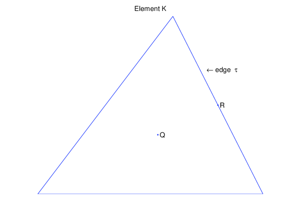
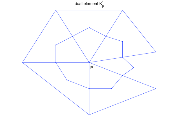
Let $T_{H}$ be a quasi-uniform triangulation of the polygonal domain $\Omega$. The barycenter dual decomposition $T_{H}^{*}$ is constructed by connecting the barycenter to the midpoints of edges of every triangle element by straight lines. Given a triangle element $K$, let $\tau$ and $Q$ be an edge and barycenter, respectively, of $K$, $R$ be the midpoint of $\tau$. Next, let $P$ be a modal point and $K_{P}^{*}$ be the dual element with respect to $P$ (see Figure 1). Denote by $H$ the maximum length of the edges, $N_{H}$ the set of all nodal points. And denote by $\dot{K}$ the vertices of $K$.

Refer to caption
Refer to caption
Figure 1: The left figure is an element K, and the right figure represents the dual element with respect to a node P

Let $U=H_{0}^{1}(\Omega)=\{u\in H^{1}(\Omega)|u=0\;on\;\partial\Omega\}$ and $U_{H}\subset U$ be the piecewise linear finite element space on $T_{H}$. Denote by Ξ Hβˆ—superscriptsubscriptΠ𝐻\Pi_{H}^{*} the interpolation operator from $U_{H}$ to the piecewise constant space on $T_{H}^{*}$:

(Ξ Hβˆ—β€‹vH)​(x)=vH​(P),x∈KPβˆ—,βˆ€P∈NH,vH∈UH.formulae-sequencesuperscriptsubscriptΠ𝐻subscript𝑣𝐻π‘₯subscript𝑣𝐻𝑃formulae-sequenceπ‘₯superscriptsubscript𝐾𝑃formulae-sequencefor-all𝑃subscript𝑁𝐻subscript𝑣𝐻subscriptπ‘ˆπ»(\Pi_{H}^{*}v_{H})(x)=v_{H}(P),x\in K_{P}^{*},\forall P\in N_{H},v_{H}\in U_{H}.

Then the finite volume method(FVM)[17] reads as: Find $u_{H}\in U_{H}$ such that

A​(uH,Ξ Hβˆ—β€‹vH)=(f,Ξ Hβˆ—β€‹vH),βˆ€vH∈UH,formulae-sequence𝐴subscript𝑒𝐻superscriptsubscriptΠ𝐻subscript𝑣𝐻𝑓superscriptsubscriptΠ𝐻subscript𝑣𝐻for-allsubscript𝑣𝐻subscriptπ‘ˆπ»\displaystyle A(u_{H},\Pi_{H}^{*}v_{H})=(f,\Pi_{H}^{*}v_{H}),\forall v_{H}\in U_{H}, (2.1)

where

A​(uH,Ξ Hβˆ—β€‹vH)=βˆ‘P∈NH[βˆ’βˆ«βˆ‚KPβˆ—π§β‹…(aHβ€‹βˆ‡uH)​ΠHβˆ—β€‹vH​𝑑s+∫KPβˆ—(bHβ€‹βˆ‡uH+cH​uH)​ΠHβˆ—β€‹vH​𝑑x]𝐴subscript𝑒𝐻superscriptsubscriptΠ𝐻subscript𝑣𝐻subscript𝑃subscript𝑁𝐻delimited-[]subscriptsuperscriptsubscript𝐾𝑃⋅𝐧superscriptπ‘Žπ»βˆ‡subscript𝑒𝐻superscriptsubscriptΠ𝐻subscript𝑣𝐻differential-d𝑠subscriptsuperscriptsubscript𝐾𝑃superscriptπ‘π»βˆ‡subscript𝑒𝐻superscript𝑐𝐻subscript𝑒𝐻superscriptsubscriptΠ𝐻subscript𝑣𝐻differential-dπ‘₯\displaystyle A(u_{H},\Pi_{H}^{*}v_{H})=\sum_{P\in N_{H}}\left[-\int_{\partial K_{P}^{*}}\mathbf{n}\cdot(a^{H}\nabla u_{H})\Pi_{H}^{*}v_{H}ds+\int_{K_{P}^{*}}(b^{H}\nabla u_{H}+c^{H}u_{H})\Pi_{H}^{*}v_{H}dx\right]
$\displaystyle=\sum_{K\in T_{H}}\left[-\sum_{P\in\dot{K}}\int_{K\cap\partial K_{P}^{*}}\mathbf{n}\cdot(a^{H}\nabla u_{H})\Pi_{H}^{*}v_{H}ds+\int_{K}(b^{H}\nabla u_{H}+c^{H}u_{H})\Pi_{H}^{*}v_{H}dx\right],$ (2.2)

and

(f,Ξ Hβˆ—β€‹vH)=βˆ‘K∈TH∫Kf​ΠHβˆ—β€‹vH​𝑑x.𝑓superscriptsubscriptΠ𝐻subscript𝑣𝐻subscript𝐾subscript𝑇𝐻subscript𝐾𝑓superscriptsubscriptΠ𝐻subscript𝑣𝐻differential-dπ‘₯\displaystyle(f,\Pi_{H}^{*}v_{H})=\sum_{K\in T_{H}}\int_{K}f\Pi_{H}^{*}v_{H}dx. (2.3)

Consider the numerical integration for the barycenter quadrature rule, (2) and (2.3) can be written as:

AF​V​M(uH,Ξ Hβˆ—vH)=βˆ‘K∈TH[βˆ’βˆ‘P∈KΛ™|Kβˆ©βˆ‚KPβˆ—|𝐧⋅(aH(Q)βˆ‡uH)Ξ Hβˆ—vH\displaystyle A_{FVM}(u_{H},\Pi_{H}^{*}v_{H})=\sum_{K\in T_{H}}[-\sum_{P\in\dot{K}}\left|K\cap\partial K_{P}^{*}\right|\mathbf{n}\cdot(a^{H}(Q)\nabla u_{H})\Pi_{H}^{*}v_{H}
+|K|(bH(Q)βˆ‡uH+cH(Q)uH(Q))Ξ Hβˆ—vH],\displaystyle+\left|K\right|\left(b^{H}(Q)\nabla u_{H}+c^{H}(Q)u_{H}(Q)\right)\Pi_{H}^{*}v_{H}], (2.4)

and

(f,Ξ Hβˆ—β€‹vH)H=βˆ‘K∈TH|K|​f​(Q)​ΠHβˆ—β€‹vH.subscript𝑓superscriptsubscriptΠ𝐻subscript𝑣𝐻𝐻subscript𝐾subscript𝑇𝐻𝐾𝑓𝑄superscriptsubscriptΠ𝐻subscript𝑣𝐻\displaystyle(f,\Pi_{H}^{*}v_{H})_{H}=\sum_{K\in T_{H}}\left|K\right|f(Q)\Pi_{H}^{*}v_{H}. (2.5)

Thus, the barycenter quadrature approximation of the FVM reads: Find $u_{H}\in U_{H}$ such that

AF​V​M​(uH,Ξ Hβˆ—β€‹vH)=(f,Ξ Hβˆ—β€‹vH)H,βˆ€vH∈UH.formulae-sequencesubscript𝐴𝐹𝑉𝑀subscript𝑒𝐻superscriptsubscriptΠ𝐻subscript𝑣𝐻subscript𝑓superscriptsubscriptΠ𝐻subscript𝑣𝐻𝐻for-allsubscript𝑣𝐻subscriptπ‘ˆπ»\displaystyle A_{FVM}(u_{H},\Pi_{H}^{*}v_{H})=(f,\Pi_{H}^{*}v_{H})_{H},\;\;\;\forall v_{H}\in U_{H}. (2.6)

This paper considers the scale separation in the coefficients. Assume the multiscale coefficients $a^{\varepsilon}(x)$, $b^{\varepsilon}(x)$ and $c^{\varepsilon}(x)$ have the forms $a(x,\frac{x}{\varepsilon})$, $b(x,\frac{x}{\varepsilon})$ and $c(x,\frac{x}{\varepsilon})$. Moreover, assume that $a(x,y)$, $b(x,y)$ and $c(x,y)$ are smooth in $x$ and periodic in $y$ with respect to the unit cube $Y$.

In the absence of explicit knowledge of $a^{H}$, $b^{H}$ and $c^{H}$, $a^{H}(Q)\nabla u_{H}$, $b^{H}(Q)\nabla u_{H}$ and $c^{H}(Q)$ can be approximated by

$\displaystyle a^{H}(Q)\nabla u_{H}\simeq\frac{1}{|K_{\delta}(Q)|}\int_{K_{\delta}(Q)}a(Q,\frac{x}{\varepsilon})\nabla R(u_{H})dx,$ (2.7)
$\displaystyle b^{H}(Q)\nabla u_{H}\simeq\frac{1}{|K_{\delta}(Q)|}\int_{K_{\delta}(Q)}b(Q,\frac{x}{\varepsilon})\nabla R(u_{H})dx,$ (2.8)

and

$\displaystyle c^{H}(Q)\simeq\frac{1}{|K_{\delta}(Q)|}\int_{K_{\delta}(Q)}c(Q,\frac{x}{\varepsilon})dx,$ (2.9)

where $R(u_{H})$ is the solution of the following microcell problem

$$\left\{\begin{array}[]{cc}\displaystyle-\nabla\cdot(a(Q,\frac{x}{\varepsilon})\nabla R(u_{H}))=0,&\mbox{in}\;K_{\delta}(Q),\\ \displaystyle R(u_{H})=u_{H},&\mbox{on}\;\partial K_{\delta}(Q),\end{array}\right.$$ (2.10)

and $K_{\delta}(Q)$ is a cube of size $\delta$ centered at $Q$.

Thus, the HMM-FVM is defined by the following variational problem: $\forall v_{H}\in U_{H}$, find $u_{H}\in U_{H}$ that satisfies (2.6), (2.7), (2.8) and (2.9).

Our main result is the following.

Theorem 2.1

Denote by $u^{0}$ and $u_{H}$ the solution of (1.6) and (2.6), respectively. Then for sufficient small $H$ and $\varepsilon/\delta$, we have

$\displaystyle||u^{0}-u_{H}||_{1,\Omega}\leq C\left(H+\frac{\varepsilon}{\delta}\right),$

where $C$ is a positive constant independent of $\varepsilon$, $\delta$ and $H$.

3 A priori error estimate

In this section, we consider the HMM-FVM as a perturbation of the linear finite element method(FEM), and then obtain the optimal $H^{1}$ error estimate.

The finite element method for the homogenization problem (1.6) reads as: find $u_{H}\in U_{H}$ such that

$\displaystyle B(u_{H},v_{H})=(f,v_{H}),~{}~{}~{}\forall v_{H}\in U_{H},$ (3.1)

where

$\displaystyle B(u_{H},v_{H})=\sum_{K\in T_{H}}\int_{K}\left(a^{0}\nabla u_{H}\cdot\nabla v_{H}+b^{0}\nabla u_{H}v_{H}+c^{0}u_{H}v_{H}\right)dx$ (3.2)

and

$\displaystyle(f,v_{H})=\sum_{K\in T_{H}}\int_{K}fv_{H}dx.$ (3.3)

Using the barycenter quadrature into (3.2), the bilinear form can be refined by

$\displaystyle\tilde{B}(u_{H},v_{H})=\sum_{K\in T_{H}}|K|\left(a^{0}(Q)\nabla u_{H}\cdot\nabla v_{H}+b^{0}(Q)\nabla u_{H}v_{H}(Q)+c^{0}(Q)u_{H}(Q)v_{H}(Q)\right).$ (3.4)

The following Lemma characterizes the difference between the bilinear form of the HMM-FVM and that of the FEM, which plays the key role in the subsequent analysis.

Lemma 3.1

$\forall u_{H},v_{H}\in U_{H}$, we have

$\displaystyle|B(u_{H},v_{H})-A_{FVM}(u_{H},v_{H})|\leq C\left(H+\frac{\varepsilon}{\delta}\right)||u_{H}||_{1,~{}\Omega}||v_{H}||_{1,~{}\Omega},$

where $C$ is a positive constant independent of $\varepsilon$, $\delta$ and $H$.

Proof. The bilinear form can be eliminated by three terms

$\displaystyle|B(u_{H},v_{H})-A_{FVM}(u_{H},v_{H})|$ $\displaystyle\leq$ $\displaystyle|B(u_{H},v_{H})-\tilde{B}(u_{H},v_{H})|$
$\displaystyle+$ $\displaystyle|\tilde{B}(u_{H},v_{H})-\tilde{A}(u_{H},v_{H})|$
$\displaystyle+$ $\displaystyle|\tilde{A}(u_{H},v_{H})-A_{FVM}(u_{H},v_{H})|$
$\displaystyle:=$ $\displaystyle\varepsilon_{1}(u_{H},v_{H})+\varepsilon_{2}(u_{H},v_{H})+\varepsilon_{3}(u_{H},v_{H}),$

where

$\displaystyle\tilde{A}(u_{H},v_{H})=\sum_{K\in T_{H}}|K|\left(a^{H}(Q)\nabla u_{H}\cdot\nabla v_{H}+b^{H}(Q)\nabla u_{H}v_{H}(Q)+c^{H}(Q)u_{H}(Q)v_{H}(Q)\right).$ (3.5)

Denote by

$\displaystyle E_{K}(f)=\int_{K}f(x)dx-|K|f(Q),$ (3.6)

then from the standard estimate[6]

$\displaystyle|E_{K}(a(x)p(x)q(x))|\leq CH||a||_{1,~{}\infty}||p||_{0,~{}K}||q||_{0,~{}K},$ (3.7)

the numerical quadrature error $\varepsilon_{1}(u_{H},v_{H})$ can be easily estimated as

$\displaystyle\varepsilon_{1}(u_{H},v_{H})$ $\displaystyle\leq$ $\displaystyle\sum_{K\in T_{H}}\left(|E_{K}(a^{0}\nabla u_{H}\cdot\nabla v_{H})|+|E_{K}(b^{0}u_{H}\nabla v_{H})|+|E_{K}(c^{0}u_{H}v_{H})|\right)$ (3.8)
$\displaystyle\leq$ $\displaystyle CH||u_{H}||_{1,~{}\Omega}||v_{H}||_{1,~{}\Omega}.$ (3.9)

In order to estimate the modeling error $\varepsilon_{2}(u_{H},v_{H})$, the following Lemmas are useful.

Lemma 3.2

([4, 11, 16]) There exists a constant $C$ independent of H, $\varepsilon$ and $\delta$ such that for $a^{H}$, $b^{H}$,

$\displaystyle\left|a^{H}_{ij}-a^{0}_{ij}\right|\leq C\frac{\varepsilon}{\delta},\;\;i,j=1,2,$

and

$\displaystyle\left|b^{H}_{i}-b^{0}_{i}\right|\leq C\frac{\varepsilon}{\delta},\;\;i=1,2.$
Lemma 3.3

([4, 5]) Given domain $K_{\delta}$ with $diam(K)=\delta$, let φ​(s,y)πœ‘π‘ π‘¦\varphi(s,y) defined in $Y$ be a $Y-$periodic function in $y$, where $Y$ is a unit cube and $s\in R$ is fixed. Then

|1|Y|β€‹βˆ«Yφ​(s,y)​𝑑yβˆ’<φ​(s,x/Ξ΅)>K|≀C​Ρδ,1π‘Œsubscriptπ‘Œπœ‘π‘ π‘¦differential-d𝑦subscriptexpectationπœ‘π‘ π‘₯πœ€πΎπΆπœ€π›Ώ\displaystyle\left|\frac{1}{|Y|}\int_{Y}\varphi(s,y)dy-<\varphi(s,x/\varepsilon)>_{K}\right|\leq C\frac{\varepsilon}{\delta},

where $C$ is independent of $\varepsilon$, $\delta$ and $s$.

Directly from the definition of $c^{H}$ in (2.9) and Lemma 3.3, the error between $c^{H}$ and $c^{0}$ can be easily estimate as

$\displaystyle\left|c^{H}-c^{0}\right|\leq C\frac{\varepsilon}{\delta},$ (3.10)

where $C$ is a positive constant independent of $\varepsilon$, $\delta$ and $H$.

Denote by

$$e(HMM)=\max_{x\in\Omega}\left\{\left|a^{H}_{ij}-a^{0}_{ij}\right|,\left|b^{H}_{i}-b^{0}_{i}\right|,\left|c^{H}-c^{0}\right|\right\},$$

then

$\displaystyle e(HMM)\leq C\frac{\varepsilon}{\delta}$ (3.11)

from Lemma 3.2 and (3.10).
So the modeling error $\varepsilon_{2}(u_{H},v_{H})$ can be estimate as

$\displaystyle\varepsilon_{2}(u_{H},v_{H})\leq Ce(HMM)||u_{H}||_{1,~{}\Omega}||v_{H}||_{1,~{}\Omega}\leq C\frac{\varepsilon}{\delta}||u_{H}||_{1,~{}\Omega}||v_{H}||_{1,~{}\Omega}.$ (3.12)

It remains to estimate the term $\varepsilon_{3}(u_{H},v_{H})$. Deduce by Green’s formula, the first term of $\tilde{A}(u_{H},v_{H})$ reads

$\displaystyle|K|a^{H}(Q)\nabla u_{H}\nabla v_{H}$ $\displaystyle=$ $\displaystyle\int_{K}a^{H}(Q)\nabla u_{H}\nabla v_{H}dx$
$\displaystyle=$ $\displaystyle-\int_{K}\nabla(a^{H}(Q)\nabla u_{H})v_{H}dx+\int_{\partial K}n\cdot(a^{H}(Q)\nabla u_{H})v_{H}ds$
$\displaystyle=$ $\displaystyle\int_{\partial K}n\cdot(a^{H}(Q)\nabla u_{H})v_{H}ds$

The first term of $A_{FVM}(u_{H},v_{H})$ can derived similarly

$\displaystyle-$ $\displaystyle\sum_{P\in\dot{K}}|K\cap\partial K_{P}^{*}|n\cdot(a^{H}(Q)\nabla u_{H})\Pi_{H}^{*}v_{H}$
$\displaystyle=$ $\displaystyle-\sum_{P\in\dot{K}}\int_{K\cap\partial K_{P}^{*}}n\cdot(a^{H}(Q)\nabla u_{H})\Pi_{H}^{*}v_{H}ds$
$\displaystyle=$ $\displaystyle-\sum_{P\in\dot{K}}\int_{\partial(K\cap\partial K_{P}^{*})}n\cdot(a^{H}(Q)\nabla u_{H})\Pi_{H}^{*}v_{H}ds+\int_{\partial K}n\cdot(a^{H}(Q)\nabla u_{H})\Pi_{H}^{*}v_{H}ds$
$\displaystyle=$ $\displaystyle-\int_{K}\nabla(a^{H}(Q)\nabla u_{H})\Pi_{H}^{*}v_{H}dx+\int_{\partial K}n\cdot(a^{H}(Q)\nabla u_{H})\Pi_{H}^{*}v_{H}ds$
$\displaystyle=$ $\displaystyle\int_{\partial K}n\cdot(a^{H}(Q)\nabla u_{H})\Pi_{H}^{*}v_{H}ds$

Thus by (3.11) and the property of the operator Ξ Hβˆ—superscriptsubscriptΠ𝐻\Pi_{H}^{*} (see Lemma 2.1 in [17])

β€–vHβˆ’Ξ Hβˆ—β€‹vHβ€–0,K≀C​H​|vH|1,K,βˆ€vH∈UH,formulae-sequencesubscriptnormsubscript𝑣𝐻superscriptsubscriptΠ𝐻subscript𝑣𝐻0𝐾𝐢𝐻subscriptsubscript𝑣𝐻1𝐾for-allsubscript𝑣𝐻subscriptπ‘ˆπ»\displaystyle||v_{H}-\Pi_{H}^{*}v_{H}||_{0,K}\leq CH|v_{H}|_{1,K},\;\;\forall v_{H}\in U_{H}, (3.13)

the last term $\varepsilon_{3}(u_{H},v_{H})$ can be estimated as

$\displaystyle\varepsilon_{3}(u_{H},v_{H})\!\!\!$ $\displaystyle=$ βˆ‘K∈TH[βˆ‘eβˆˆβˆ‚K∫enβ‹…(aH(Q)βˆ‡uH)(vHβˆ’Ξ Hβˆ—vH)ds\displaystyle\!\!\!\sum_{K\in T_{H}}[\sum_{e\in\partial K}\int_{e}n\cdot(a^{H}(Q)\nabla u_{H})(v_{H}-\Pi_{H}^{*}v_{H})ds
+|K|(bH(Q)βˆ‡uH+cH(Q)uH)(vHβˆ’Ξ Hβˆ—vH)]\displaystyle\!\!\!+|K|\left(b^{H}(Q)\nabla u_{H}+c^{H}(Q)u_{H}\right)(v_{H}-\Pi_{H}^{*}v_{H})]
$\displaystyle=$ βˆ‘K∈TH|K|​(bH​(Q)β€‹βˆ‡uH+cH​(Q)​uH)​(vHβˆ’Ξ Hβˆ—β€‹vH)subscript𝐾subscript𝑇𝐻𝐾superscriptπ‘π»π‘„βˆ‡subscript𝑒𝐻superscript𝑐𝐻𝑄subscript𝑒𝐻subscript𝑣𝐻superscriptsubscriptΠ𝐻subscript𝑣𝐻\displaystyle\!\!\!\sum_{K\in T_{H}}|K|\left(b^{H}(Q)\nabla u_{H}+c^{H}(Q)u_{H}\right)(v_{H}-\Pi_{H}^{*}v_{H})
$\displaystyle\leq$ βˆ‘K∈TH|K|​(β€–bHβ€–0,∞,Kβ€‹β€–βˆ‡uHβ€–0,∞,K+β€–cHβ€–0,∞,K​‖uHβ€–0,∞,K)​‖vHβˆ’Ξ Hβˆ—β€‹vHβ€–0,∞,Ksubscript𝐾subscript𝑇𝐻𝐾subscriptnormsuperscript𝑏𝐻0𝐾subscriptnormβˆ‡subscript𝑒𝐻0𝐾subscriptnormsuperscript𝑐𝐻0𝐾subscriptnormsubscript𝑒𝐻0𝐾subscriptnormsubscript𝑣𝐻superscriptsubscriptΠ𝐻subscript𝑣𝐻0𝐾\displaystyle\!\!\!\sum_{K\in T_{H}}|K|\left(||b^{H}||_{0,\infty,K}||\nabla u_{H}||_{0,\infty,K}+||c^{H}||_{0,\infty,K}||u_{H}||_{0,\infty,K}\right)||v_{H}-\Pi_{H}^{*}v_{H}||_{0,\infty,K}
$\displaystyle\leq$ Cβ€‹βˆ‘K∈TH(β€–bHβ€–0,∞,Kβ€‹β€–βˆ‡uHβ€–0,2,K+β€–cHβ€–0,∞,K​‖uHβ€–0,2,K)​‖vHβˆ’Ξ Hβˆ—β€‹vHβ€–0,2,K𝐢subscript𝐾subscript𝑇𝐻subscriptnormsuperscript𝑏𝐻0𝐾subscriptnormβˆ‡subscript𝑒𝐻02𝐾subscriptnormsuperscript𝑐𝐻0𝐾subscriptnormsubscript𝑒𝐻02𝐾subscriptnormsubscript𝑣𝐻superscriptsubscriptΠ𝐻subscript𝑣𝐻02𝐾\displaystyle\!\!\!C\sum_{K\in T_{H}}\left(||b^{H}||_{0,\infty,K}||\nabla u_{H}||_{0,2,K}+||c^{H}||_{0,\infty,K}||u_{H}||_{0,2,K}\right)||v_{H}-\Pi_{H}^{*}v_{H}||_{0,2,K}
$\displaystyle\leq$ C​(β€–bHβ€–0,∞,Ξ©+β€–cHβ€–0,∞,Ξ©)​‖uHβ€–1,Ω​‖vHβˆ’Ξ Hβˆ—β€‹vHβ€–0,Ω𝐢subscriptnormsuperscript𝑏𝐻0Ξ©subscriptnormsuperscript𝑐𝐻0Ξ©subscriptnormsubscript𝑒𝐻1Ξ©subscriptnormsubscript𝑣𝐻superscriptsubscriptΠ𝐻subscript𝑣𝐻0Ξ©\displaystyle\!\!\!C\left(||b^{H}||_{0,\infty,\Omega}+||c^{H}||_{0,\infty,\Omega}\right)||u_{H}||_{1,\Omega}||v_{H}-\Pi_{H}^{*}v_{H}||_{0,\Omega}
$\displaystyle\leq$ $\displaystyle\!\!\!CH\left(||b^{H}||_{0,\infty,\Omega}+||c^{H}||_{0,\infty,\Omega}\right)||u_{H}||_{1,\Omega}|v_{H}|_{1,\Omega}$
$\displaystyle\leq$ $\displaystyle\!\!\!CH\left(||b^{0}||_{0,\infty,\Omega}+||c^{0}||_{0,\infty,\Omega}+e(HMM)\right)||u_{H}||_{1,\Omega}|v_{H}|_{1,\Omega}$
$\displaystyle\leq$ $\displaystyle\!\!\!C\left(H+e(HMM)\right)||u_{H}||_{1,\Omega}|v_{H}|_{1,\Omega}$
$\displaystyle\leq$ $\displaystyle\!\!\!C\left(H+\frac{\varepsilon}{\delta}\right)||u_{H}||_{1,\Omega}|v_{H}|_{1,\Omega}.$

Therefore, by the estimate of $\varepsilon_{1}(u_{H},v_{H})$, $\varepsilon_{2}(u_{H},v_{H})$ and $\varepsilon_{3}(u_{H},v_{H})$, we obtain

$\displaystyle|B(u_{H},v_{H})-A_{FVM}(u_{H},v_{H})|\leq C\left(H+\frac{\varepsilon}{\delta}\right)||u_{H}||_{1,~{}\Omega}||v_{H}||_{1,~{}\Omega}$

Β 

In order to estimate the error between $u^{0}$ and $u^{H}$, we separate it into two parts

$\displaystyle||u^{0}-u_{H}||_{1,\Omega}\!\!\!$ $\displaystyle\leq$ $\displaystyle\!\!\!||u^{0}-u^{0}_{H}||_{1,\Omega}+||u^{0}_{H}-u_{H}||_{1,\Omega},$

where $u^{0}_{H}$ is the numerical solution of (3.1), which is FEM formula of the homogenized problem (1.6). From the standard error estimate, we have

$\displaystyle||u^{0}-u^{0}_{H}||_{1,\Omega}\leq CH||u^{0}||_{1,\Omega}.$ (3.14)

To estimate $||u^{0}_{H}-u_{H}||_{1,\Omega}$, the inf-sup condition for bilinear form $B$ in [17] is useful.

Lemma 3.4

[17] For $0<H<h_{0}$, we have

β€–uHβ€–1,Ω≀C​sup0β‰ vH∈UHB​(uH,vH)β€–vHβ€–1,Ξ©,βˆ€uH∈UH.formulae-sequencesubscriptnormsubscript𝑒𝐻1Ω𝐢subscriptsupremum0subscript𝑣𝐻subscriptπ‘ˆπ»π΅subscript𝑒𝐻subscript𝑣𝐻subscriptnormsubscript𝑣𝐻1Ξ©for-allsubscript𝑒𝐻subscriptπ‘ˆπ»\displaystyle||u_{H}||_{1,\Omega}\leq C\sup_{0\neq v_{H}\in U_{H}}\frac{B(u_{H},v_{H})}{||v_{H}||_{1,\Omega}},~{}\forall u_{H}\in U_{H}.

Then the second part can be derived as

$\displaystyle||u^{0}_{H}-u_{H}||_{1,\Omega}\!\!\!$ $\displaystyle\leq$ C​sup0β‰ vH∈UHB​(uH0βˆ’uH,vH)β€–vHβ€–1,Ω𝐢subscriptsupremum0subscript𝑣𝐻subscriptπ‘ˆπ»π΅subscriptsuperscript𝑒0𝐻subscript𝑒𝐻subscript𝑣𝐻subscriptnormsubscript𝑣𝐻1Ξ©\displaystyle\!\!\!C\sup_{0\neq v_{H}\in U_{H}}\frac{B(u^{0}_{H}-u_{H},v_{H})}{||v_{H}||_{1,\Omega}} (3.15)
$\displaystyle\leq$ C​sup0β‰ vH∈UH(|B​(uH,vH)βˆ’AF​V​M​(uH,Ξ Hβˆ—β€‹vH)|β€–vHβ€–1,Ξ©+|(f,vH)Hβˆ’(f,Ξ Hβˆ—β€‹vH)H|β€–vHβ€–1,Ξ©)𝐢subscriptsupremum0subscript𝑣𝐻subscriptπ‘ˆπ»π΅subscript𝑒𝐻subscript𝑣𝐻subscript𝐴𝐹𝑉𝑀subscript𝑒𝐻superscriptsubscriptΠ𝐻subscript𝑣𝐻subscriptnormsubscript𝑣𝐻1Ξ©subscript𝑓subscript𝑣𝐻𝐻subscript𝑓superscriptsubscriptΠ𝐻subscript𝑣𝐻𝐻subscriptnormsubscript𝑣𝐻1Ξ©\displaystyle\!\!\!C\sup_{0\neq v_{H}\in U_{H}}\left(\frac{|B(u_{H},v_{H})-A_{FVM}(u_{H},\Pi_{H}^{*}v_{H})|}{||v_{H}||_{1,\Omega}}+\frac{|(f,v_{H})_{H}-(f,\Pi_{H}^{*}v_{H})_{H}|}{||v_{H}||_{1,\Omega}}\right)
$\displaystyle:=$ $\displaystyle\!\!\!T_{1}+T_{2}.$

By Lemma 3.1, we can easily obtain

$\displaystyle T_{1}\!\!\!$ $\displaystyle\leq$ $\displaystyle\!\!\!C\left(H+\frac{\epsilon}{\delta}\right)||u_{H}||_{1,\Omega}$ (3.16)
$\displaystyle\leq$ $\displaystyle\!\!\!C\left(H+\frac{\epsilon}{\delta}\right)\left(||u^{0}||_{1,\Omega}+||u_{H}-u^{0}||_{1,\Omega}\right).$

Denote by

$\displaystyle\varepsilon(f)\!\!\!$ $\displaystyle=$ (f,vH)Hβˆ’(f,Ξ Hβˆ—β€‹vH)H=βˆ‘K∫Kf​vH​𝑑xβˆ’βˆ‘K|K|​f​(Q)​ΠHβˆ—β€‹vHsubscript𝑓subscript𝑣𝐻𝐻subscript𝑓superscriptsubscriptΠ𝐻subscript𝑣𝐻𝐻subscript𝐾subscript𝐾𝑓subscript𝑣𝐻differential-dπ‘₯subscript𝐾𝐾𝑓𝑄superscriptsubscriptΠ𝐻subscript𝑣𝐻\displaystyle\!\!\!(f,v_{H})_{H}-(f,\Pi_{H}^{*}v_{H})_{H}=\sum_{K}\int_{K}fv_{H}dx-\sum_{K}|K|f(Q)\Pi_{H}^{*}v_{H}
$\displaystyle=$ $\displaystyle\!\!\!\sum_{K}\int_{K}fv_{H}dx-\sum_{K}\int_{K}f(Q)\Pi_{H}^{*}v_{H}dx=\sum_{K}\int_{K}fv_{H}dx-\sum_{K}\int_{K}f(Q)v_{H}dx$
$\displaystyle=$ $\displaystyle\!\!\!\sum_{K}\int_{K}(f(x)-f(Q))v_{H}dx\leq CH\sum_{K}||\nabla f||_{0,2,K}||v_{H}||_{0,2,K}$
$\displaystyle\leq$ $\displaystyle\!\!\!CH|f|_{1,\Omega}||v_{H}||_{0,\Omega}\leq CH|f|_{1,\Omega}||v_{H}||_{1,\Omega},$

then

$\displaystyle T_{2}\leq CH|f|_{1,\Omega}.$ (3.17)

Therefor, from (3.14), (3.15), (3.16) and (3.17), we have

$\displaystyle||u^{0}-u_{H}||_{1,\Omega}\leq C\left(H+\frac{\varepsilon}{\delta}\right).$

Β 

Acknowledgments

This work is supported in part by the Doctoral Starting up Foundation of Jinggangshan University under the Grant JZB11002.

References

  • [1] I. BabuΕ‘ka and J.E. Osborn, Generalized finite element methods: their performance and their relation to mixed methods, SIAM J. Numer. Anal., 20(3)(1983)510-536.
  • [2] A. Bensoussan, J.-L. Lions and G. Papanicolaou, Asymptotic Analysis for Periodic Structures, Studies in Mathematics and its Applications, vol. 5, North-Holland Publ., New York, 1978.
  • [3] J. Bear, Dynamics of Fluids in Porous Media, American Elsevier, New York, 1972.
  • [4] Z.M. Chen, W.B. Deng and H. Ye, A new upscaling method for the solute transport equations, Discrete Contin. Dyn. Syst., Ser. A 13(4)(2005)941-960.
  • [5] Z.M. Chen, W.B. Deng and H. Ye, Upscaling of a class of nonlinear parabolic equtions for the flow transport in heterogeneous porous media, Commun. Math. Sci., 3(4)(2005)479-680.
  • [6] P.G. Clarlet, The finite element method for elliptic problems, North-Holland, Amsterdam, New York, Oxford, 1978.
  • [7] L.J. Durlofsky, Numerical calculation of equivalent grid block permeability tensors for heterogeneous porous media, Water Ressour. Res., 27(1991)699-708.
  • [8] W.B. Deng, J. Gu and J.M. Huang, Upscaling methods for a class of convection-diffusion equations with highly oscillating coefficients, J. Comput. Phys., 227(2008)7621-7642.
  • [9] W.B. Deng, X.L. Yun and C.H. Xie, Convergence analysis of the multiscale method for a class of convection-diffusion equations with highly oscillating coefficients, Appl. Numer. Math., 59(7)(2009)1549-1567.
  • [10] W. E and B. Engquist, The heterogeneous multi-scale methods, Commun. Math. Sci., 1(2003)87-132
  • [11] W. E, P. Ming and P. Zhang, Analysis of the heterogeneous multiscale methods for elliptic homogenization problems, J. Amer. Math. Soc., 18(2005)121-156.
  • [12] L.P. Franca and A. Russo, Deriving upwinding, mass lumping and selective reduced integration by residual-free bubbles, Appl. Math. Lett. 9(5)(1996)83-88.
  • [13] T.Y. Hou and X.H. Wu, A multiscale finite element method for elliptic problems in composite materials and porous media, J. Comput. Phys.,134(1997)169 C189.
  • [14] T.J.R. Hughes, Multiscale phenomena: Green’s functions, the Dirichlet to Neumann formulation, subgrid scale models, bubbles and the origin of stabilized methods, Comput. Meth. Appl. Mech. Eng. 127(1995)387-401.
  • [15] V.V. Jikov, S.M. Kozlov and O.A. Oleinik, Homogenization of Differential Operators and Integral Functionals, Springer-Verlag, Berlin, 1994.
  • [16] X.H. Wu, Y. Efendiev and T.Y. Hou, Analysis of upscaling absolute permeability, Discrete Contin. Dyn. Syst. Ser. B, 2(2002)185-204.
  • [17] H.J. Wu and R.H. Li, Error Estimates for Finite Volume Element Methods for General Second-Order Elliptic Problems, Numerical Methods for Partial Differential Equations, 19:6(2003)693-708.