Molecular chains interacting by Lennard-Jones and Coulomb forces

Abstract

We study equations for the mechanical movement of chains of identical particles in the plane interacting with their nearest-neighbors by bond stretching and by van der Waals and Coulomb forces. We find collinear and circular equilibria as minimizers of the energy potential for chains with Neumann and periodic boundary conditions. We prove global bifurcation of periodic brake orbits from these equilibria applying the global Rabinowitz alternative. These results are complemented with numeric computations for ranges of parameters that include carbon atoms among other molecules.

Keywords: Lennard–Jones body problem, ring configuration, periodic solutions, global bifurcation, molecular dynamics.

MSC 34C25, 37G40, 47H11, 70H33

Introduction

Molecular mechanics have been very successful in describing both small molecules and large biological systems. They are built on the framework of classical mechanics, and rely on the accurate description of atomic interactions. The potential energy of all systems in molecular mechanics is represented by what in chemistry is known as a force field, which refers to the functional form of the potential energy and the set of parameters (e.g. bond strength, electric charge, van der Waals radius, etc.) that describe how the particles of a given system interact. Numerous force fields have been developed, from “all-atom” to “coarse-grained”. The first ones take into account every atom in a system, and the second ones treat groups of atoms as single particles (see [15] and [12] for review and state of the art).

Most classical force fields used in molecular mechanics have potential energy terms associated with bond deformations, electrostatic interactions, and van der Waals forces. We consider a chain of identical particles in the plane $u_{j}\in\mathbb{R}^{2}$ for $j=1,...,n$, where each particle $u_{j}$ interacts with its nearest neighbors $u_{j-1}$ and $u_{j+1}$ by bond stretching (no bending forces are considered), and with the rest of the chain by van der Waals and electrostatic forces, modeled with Lennard-Jones and Coulomb potentials.

The adimensionalized equations for the system of $n$ particles are

$$\ddot{u}_{j}=-V_{u_{j}},\text{\qquad}j=1,\ldots,n\text{,}$$ (1)

where the energy function is

$$V=\sum_{j=1}^{n-1}U(\left|u_{j+1}-u_{j}\right|^{2})+\sigma U(\left|u_{n}-u_{1}\right|^{2})+\sum_{1\leq j<k\leq n}W(\left|u_{j}-u_{k}\right|^{2}).$$ (2)

Bond stretching is represented by the potential

$$U(x)=x-2x^{1/2}\text{,}$$ (3)

while non-bonded interactions by a potential $W\in C^{2}$ such that

$$\lim_{x\rightarrow 0}W(x)=\lim_{x\rightarrow 0}-W^{\prime}(x)=\infty,\qquad\lim_{x\rightarrow\infty}W(x)=\lim_{x\rightarrow\infty}W^{\prime}(x)=0\text{.}$$ (4)

The assumptions for $W$ assure that the interaction is repulsive when two particles are close and vanish when they are far from each other, which is the case of van der Waals and electrostatic interactions.

Two kind of molecular chains are studied: the circular chain (periodic boundary condition), where $\sigma=1$ in (2), and the collinear chain (Neumann boundary conditions), where $\sigma=0$ in (2). The equations for the circular chain are equivariant under the symmetry group

$$D_{n}\times O(2)\times O(2)\text{,}$$

which acts by permuting particles, rotating positions and translating time; see (5) and (8) for details. For the collinear chain, the equations are equivariant only under the group $\mathbb{Z}_{2}\times O(2)\times O(2)$.

In Theorem 1, we use the Palais principle of symmetric criticality to obtain equilibria as minimizers of $V$ in subspaces of symmetric configurations. This allows us to prove the existence of symmetric collinear and circular equilibria, among others.

Theorems 11 and 13 establish that both the collinear and circular equilibria have a global bifurcation of $2\pi/\nu$-periodic solutions emanating from the frequency $\nu=\nu_{0}$ for each positive non-resonant eigenvalue $\nu_{0}^{2}$ of the Hessian of $V$. The global property is proved using the global Rabinowitz alternative in subspaces of symmetric periodic functions. This property assures us that the branch is a continuum. Moreover, the branch has norm or period going to infinity, ends in a collision, or comes back to other bifurcation point.

The solutions given in Theorems 11 and 13 are brake orbits (Figure 1). These kind of orbits are solutions for which all the velocities are zero at some instant, see [2], [13] and references therein. Bifurcation of other types of periodic solutions for molecules have been considered previously in [11].

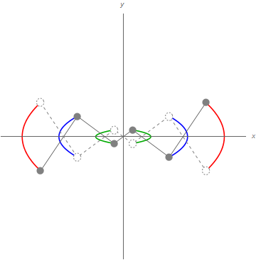
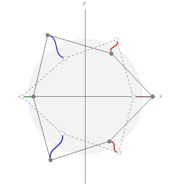
Figure 1: Illustration of the symmetries of brake orbits for $n=6$. Orbits with the same color are symmetric by reflections and rotations.

We complement our results with numeric computations for parameters that include carbon atoms, among other particles considered in CHARMM36 force field [3]. In Figures 2 and 3, we present the amplitude of the collinear and circular equilibria for $n=6$, respectively, and the number of negative eigenvalues of the Hessian. The numeric computations allow us to conclude that both equilibria for $6$ general particles loose stability when the Lennard-Jones parameter $A$ is increased. In Table 1, we present the number of negative eigenvalues of the collinear and circular equilibria for different number of carbon atoms.

In Section 1, we prove the existence of minimizers that correspond to equilibria. In Section 2, we find the linearization around them. In Section 3, we prove global bifurcation of periodic solutions. In Section 4, we numerically estimate the amplitude and spectra of the equilibria for $n=6$, and we discuss their stability.

1 Equilibria of molecular chains

Equilibrium configurations of molecular chains correspond to critical points of $V$; these are points $\mathbf{a}=(a_{1},...,a_{n})\in\mathbb{R}^{2n}$ such that $\nabla_{u}V(\mathbf{a})=0$.

The potential $V$ is well defined in the set $\Omega=\{u\in\mathbb{R}^{2n}:u_{j}\neq u_{k}\}$. Given that any translation of an equilibrium is an equilibrium, we restrict the potential $V$ to the subspace

$$\Omega_{0}=\{u\in\Omega:\sum_{j=1}^{n}u_{j}=0\}\text{.}$$

We define the action of the group $S_{n}$ of permutations of $\{1,...,n\}$ and the group $O(2)=S^{1}\cup\tilde{\kappa}S^{1}$in $\mathbb{R}^{2n}$ as

$$\rho(\gamma)x_{j}=x_{\gamma(j)}\text{,\qquad}\rho(\theta)x_{j}=e^{-J\theta}x_{j}\text{,\qquad}\rho(\tilde{\kappa})x_{j}=Rx_{j}\text{,}$$ (5)

where the matrices $J$ and $R$ are

$$J=\left(\begin{array}[c]{cc}0&-1\\ 1&0\end{array}\right)\text{ and }R=\left(\begin{array}[c]{cc}1&0\\ 0&-1\end{array}\right)\text{.}$$

Let us assume for the moment that $V$ is $G$-invariant, where $G$ is a subgroup of $S_{n}\times O(2)$.

Theorem 1

If $H$ is a subgroup of $G$, then the minimizer of $V$ is achieved in each connected component of

$$\Omega_{0}^{H}=\Omega_{0}\cap\mathrm{Fix}(H)=\{u\in\Omega_{0}:\rho(g)u=u\text{ for }g\in H\}\text{.}$$

These minimizers are critical points of $V$ in $\Omega$.

Proof. The restricted potential $V:\Omega_{0}\subset\mathbb{R}^{2(n-1)}\rightarrow\mathbb{R}$ satisfies $V(u)\rightarrow+\infty$ when $u_{j}\rightarrow u_{j+1}$, since the non-bonded interactions are such that $\lim_{x\rightarrow 0}W(x)=\infty$. Also, given that $\lim_{x\rightarrow\infty}U(x)=\infty$, then $V(u)\rightarrow+\infty$ when $u\rightarrow\infty$. Therefore, the potential $V$ is coercive and goes to infinity in the boundary of $\Omega_{0}$. We conclude that $V$ has a minimizer in each connected component of $\Omega_{0}^{H}$.

By the Palais principle of symmetric criticality [14], each minimizer is a critical point of $V$ in $\Omega_{0}$. Moreover, a critical point of $V$ in $\Omega_{0}$ satisfies $\nabla V(\mathbf{a})+\lambda_{1}\mathbf{e}_{1}+\lambda_{2}\mathbf{e}_{2}=0$ with $\mathbf{a}\in\Omega_{0}$. The invariance of $V$ under translations implies that $\nabla V(\mathbf{a})\cdot\mathbf{e}_{j}=0$ for $j=1,2$, so $\lambda_{j}=0$. Consequently, a minimizer of $V$ in a connected component of $\Omega_{0}^{H}$ is a critical point of $V$ in $\Omega$, i.e. $\nabla V(\mathbf{a})=0$.   

We have used the property of stratification of space to guaranty the existence of a different equilibrium for each maximal isotropy group $H$ of $G$.

1.1 The collinear chain

In the case of Neumann conditions ($\sigma=0$), the potential $V$ is invariant under the group

$$G=\mathbb{Z}_{2}(\kappa)\times O(2)\text{,}$$

where $\mathbb{Z}_{2}(\kappa)$ is the group generated by the permutation given by

$$\kappa(j)=n+1-j\text{.}$$

Therefore, the minimizer of $V$ is achieved in each connected component of $\Omega_{0}^{H}$ with the maximal subgroup

$$H=\mathbb{Z}_{2}(\kappa,\pi)\times\mathbb{Z}_{2}(\tilde{\kappa})\text{.}$$

Since $(\kappa,\pi)$ and $\tilde{\kappa}$ generate $H$, the minimizer $\mathbf{a}$ in the fixed point space have components $a_{j}\in\mathbb{R}$ and $a_{n+1-j}=-a_{j}$.

In fact, the domain $\Omega_{0}^{H}$ has many connected components. Since, in the chain, $u_{j}$ is coupled only to the adjacent $u_{j-1}$ and $u_{j+1}$, we only consider the component

$$\left\{u\in\Omega_{0}\cap\mathrm{Fix}(H):u_{j}<u_{j+1}\right\}\text{,}$$

which has physical meaning.

Corollary 2

There is a symmetric collinear equilibrium $\mathbf{a}=(a_{1},...,a_{n})$ such that $a_{j}\in\mathbb{R}$ satisfy

$$a_{1}<a_{2}<...<a_{n}\text{,}$$

where $a_{1}=-a_{n}$, $a_{2}=-a_{n-1}$, etc.

Since $\mathbf{a}$ is a minimizer in $\Omega_{0}^{H}$, whose dimension is bigger than $(n-1)/2$, then the Hessian $D^{2}V(\mathbf{a)}$ has at least $(n-1)/2$ positive eigenvalues.

1.2 The circular chain

For periodic boundary conditions ($\sigma=1$), the potential $V$ is invariant under the group

$$G=D_{n}\times O(2)\text{,}$$

where $D_{n}$ is the group generated by the permutations

$$\zeta(j)=j+1,\qquad\kappa(j)=n-j\text{,}$$

modulus $n$.

Then, there is a minimizer with isotropy group

$$\tilde{D}_{n}=\left\langle(\zeta,\zeta),(\kappa,\tilde{\kappa})\right\rangle<G\text{,}$$

where $\zeta=2\pi/n$.

Definition 3

Let

$$s_{k}=2\sin\frac{k\zeta}{2}=2\sin\frac{k\pi}{n}\text{.}$$

Then, $s_{k}^{2}=s_{-k}^{2}$ and

$$\left|1-e^{ik\zeta}\right|^{2}=2(1-\cos k\zeta)=4\sin^{2}k\zeta/2=s_{k}^{2}\text{.}$$

We describe the circular equilibrium explicitly in the following proposition.

Proposition 4

We define $a_{j}=ae^{ij\zeta}$ for $j=1,...,n$ with $\zeta=2\pi/n$, where we have identified the complex plane with the real plane. Let $a$ be such that

$$U^{\prime}\left(a^{2}s_{1}^{2}\right)=-\frac{1}{2s_{1}^{2}}\sum_{k=1}^{n-1}W^{\prime}\left(a^{2}s_{k}^{2}\right)s_{k}^{2}\text{,}$$

then $\mathbf{a}=(a_{1},...,a_{n})$ is a critical point of $V$.

Proof. We have that

$$a_{j}-a_{k}=a_{j}(1-e^{i(k-j)\zeta})\text{ and }\left|a_{j}-a_{k}\right|=as_{k-j}\text{.}$$

Then

$$\sum_{k=j\pm 1}U^{\prime}(\left|a_{j}-a_{k}\right|^{2})2\left(a_{j}-a_{k}\right) =a_{j}U^{\prime}\left(a^{2}s_{1}^{2}\right)\sum_{k=j\pm 1}2(1-e^{i(k-j)\zeta})$$

$$=a_{j}U^{\prime}\left(a^{2}s_{1}^{2}\right)\left(2s_{1}^{2}\right)\text{,}$$

and

$$\sum_{k\neq j}W^{\prime}(\left|a_{j}-a_{k}\right|^{2})2\left(a_{j}-a_{k}\right) =a_{j}\sum_{k=1(k\neq j)}^{n}W^{\prime}\left(a^{2}s_{k-j}^{2}\right)2(1-e^{i(k-j)\zeta})$$

$$=a_{j}\left(\sum_{k=1}^{n-1}W^{\prime}\left(a^{2}s_{k}^{2}\right)s_{k}^{2}\right)\text{.}$$

Therefore, the derivative of $V$ at $\mathbf{a}$ is

$$V_{u_{j}}(\mathbf{a})=a_{j}\left(2U^{\prime}\left(a^{2}s_{1}^{2}\right)s_{1}^{2}+\sum_{k=1}^{n-1}W^{\prime}\left(a^{2}s_{k}^{2}\right)s_{k}^{2}\right)\text{.}$$

The proposition follows from observing that the term in parenthesis is independent of $j$.   

The previous proposition is independent of the particular form of the potentials $U$ and $W$. For the bonding potential we have $U^{\prime}(x)=1-x^{-1/2}$.

Corollary 5

Let

$$S(a)=\frac{1}{as_{1}}-\frac{1}{2s_{1}^{2}}\sum_{k=1}^{n-1}W^{\prime}\left(a^{2}s_{k}^{2}\right)s_{k}^{2}\text{.}$$

Using the properties of $W$, we have that $S(a)\rightarrow\infty$ as $a\rightarrow 0$ and $S(a)\rightarrow 0$ as $a\rightarrow+\infty$. Then, there is at least one solution of $S(\alpha)=1$, and $\mathbf{a}=(a_{1},...,a_{n})$ is a circular equilibrium, where $a_{j}=\alpha e^{ij\zeta}$.

The polygon $\mathbf{a}$ is a local minimizer in $\Omega_{0}^{H}$. Therefore, the matrix $D^{2}V(\mathbf{a)}$ has at least $1$ positive eigenvalue.

Remark 6

Depending on the form of $W$ there may exist other circular equilibria. Other critical points different to the circular chain exist in this case; for example, there is a symmetric collinear equilibrium in the fixed point space of $H=\mathbb{Z}_{2}(\kappa,\pi)\times\mathbb{Z}_{2}(\tilde{\kappa})$.

2 Linearization

We define $A_{ij}$ as the $2\times 2$ minors of the Hessian $D^{2}V(\mathbf{a})\in M_{\mathbb{R}}(2n)$, i.e.

$$D^{2}V(\mathbf{a})=(A_{ij})_{ij=1}^{n}\text{.}$$

Due to the form of the potential $V$, the minors satisfy

$$A_{ii}=-\sum_{j\neq i}A_{ij}\text{.}$$

2.1 The collinear chain

When $\mathbf{a}$ corresponds to the collinear equilibrium, the Hessian $D^{2}V(\mathbf{a)}$ is a linear $\mathbb{Z}_{2}(\tilde{\kappa})$-equivariant map. This implies that $A_{ij}R=RA_{ij}$. Then, $A_{ij}$ is diagonal and $D^{2}V(\mathbf{a)}$ has an equivalent form as $\mathrm{diag}(M_{0},M_{1})$, where the blocks $M_{k}$ correspond to different representations of $\mathbb{Z}_{2}(\tilde{\kappa})$.

Let $\delta_{ij}=1$ if $\left|i-j\right|=1$ and $\delta_{ij}=0$ otherwise. Then

$$V=\sum_{1\leq j<k\leq n}[\delta_{jk}U+W](\left|u_{j}-u_{k}\right|^{2})\text{,}$$

where

$$[\delta_{jk}U+W](\left|u_{j}-u_{k}\right|^{2})=\delta_{jk}U(\left|u_{j}-u_{k}\right|^{2})+W(\left|u_{j}-u_{k}\right|^{2})\text{.}$$

Therefore,

$$\nabla_{u_{j}}V(u)=\sum_{k\neq j}2\left(u_{j}-u_{k}\right)[\delta_{kj}U+W]^{\prime}(\left|u_{j}-u_{k}\right|^{2})\text{.}$$

If $i\neq j$, then

$$-A_{ij} =-D_{u_{i}}\nabla_{u_{j}}V=-D_{u_{i}}2\left(u_{j}-u_{i}\right)[\delta_{ij}U+W]^{\prime}(\left|u_{j}-u_{i}\right|^{2})$$

$$=2[\delta_{ij}U+W]^{\prime}\left((a_{j}-a_{i})^{2}\right)I+4\left(a_{j}-a_{i}\right)^{2}[\delta_{ij}U+W]^{\prime\prime}(\left(a_{j}-a_{i}\right)^{2})\mathrm{diag}(1,0)\text{.}$$

Explicitly, we have the following equivalence of matrices.

Proposition 7

The matrix $D^{2}V(\mathbf{a)}$ is equivalent to

$$\mathrm{diag}(M_{0},M_{1}),$$

where $M_{0}=(a_{ij})_{i,j}^{n}$, $M_{1}=(b_{ij})_{i,j=1}^{n}$, and

$$-a_{ij}=2[\delta_{ij}U+W]^{\prime}(\left(a_{j}-a_{i}\right)^{2})+4\left(a_{j}-a_{i}\right)^{2}[\delta_{ij}U+W]^{\prime\prime}(\left(a_{j}-a_{i}\right)^{2})$$

and

$$-b_{ij}=2[\delta_{ij}U+W]^{\prime}(\left(a_{j}-a_{i}\right)^{2})$$

for $i\neq j$. Moreover, $a_{ii}=\sum_{j\neq i}-a_{ij}$ and $b_{ii}=\sum_{j\neq i}-b_{ij}$.

2.2 The circular chain

The circular chain in real coordinates is given by $\mathbf{a}=(a_{1},...,a_{n})$, where $a_{j}=ae^{Jj\zeta}e_{1}$ and $e_{1}=(1,0)\in\mathbb{R}^{2}$.

Proposition 8

Using the transform

$$T_{k}(z)=(n^{-1/2}e^{(ikI+J)\zeta}z,...,n^{-1/2}e^{n(ikI+J)\zeta}z):\mathbb{C}^{2}\rightarrow\mathbb{C}^{2n}\text{,}$$ (6)

the matrix $D^{2}V(\mathbf{a})$, as a matrix in $M_{\mathbb{C}}(2n\mathbb{)}$, satisfies that

$$D^{2}V(\mathbf{a})T_{k}(z)=T_{k}(M_{k}z),$$

i.e. the Hessian decomposes in blocks

$$M_{k}=\sum_{j=1}^{n-1}(-A_{nj})(I-e^{j(ikI+J)\zeta})\text{ for }k\in\{1,...,n\}\text{.}$$

Proof. We use that $D^{2}V(\mathbf{a})\in M_{\mathbb{R}}(2n\mathbb{)}$ is $\mathbb{Z}_{n}(\zeta,\zeta)$-equivariant. See Proposition 7 of [4].   

This formula has been used to study the stability of the polygonal equilibrium for bodies and vortices in [5, 6]. In the next proposition, we calculate $M_{k}$ explicitly.

Proposition 9

Let $\delta_{j}=1$ if $j=1,n-1$ and $\delta_{j}=0$ otherwise, and

$$b_{j}=2[\delta_{j}U+W]^{\prime}\left(a^{2}s_{j}^{2}\right),\qquad c_{j}=2s_{j}^{2}[\delta_{j}U+W]^{\prime\prime}\left(a^{2}s_{j}^{2}\right)\text{.}$$

Then,

$$M_{k}=\alpha_{k}I+\beta_{k}R-\gamma_{k}(iJ)\text{,}$$

where

$$\alpha_{k} =\sum_{j=1}^{n-1}\left(b_{j}+c_{j}\right)\left(1-\cos kj\zeta\cos j\zeta\right)\text{,}$$

$$\gamma_{k} =\sum_{j=1}^{n-1}\left(b_{j}+c_{j}\right)\sin jk\zeta\sin j\zeta\text{,}$$

$$\beta_{k} =\sum_{j=1}^{n-1}c_{j}\left(\cos jk\zeta-\cos j\zeta\right)\text{.}$$

Proof. First we need to calculate $A_{nj}=D_{u_{n}}V_{u_{j}}(\mathbf{a})$. In real coordinates, $a_{j}=ae^{Jj\zeta}e_{1}$. Then,

$$\left(a_{n}-a_{j}\right)^{T}\left(a_{n}-a_{j}\right)=a^{2}\left(I-e^{Jj\zeta}\right)^{T}e_{1}^{T}e_{1}\left(I-e^{Jj\zeta}\right)=a^{2}C_{j}\text{,}$$

where $C_{j}$ is the matrix

$$C_{j}=\left(I-e^{Jj\zeta}\right)^{T}\mathrm{diag}(1,0)\left(I-e^{Jj\zeta}\right)\text{.}$$

For $j\neq n$,

$$\nabla_{u_{n}}V(u)=\sum_{k=1}^{n-1}[\delta_{k}U+W]^{\prime}(\left|u_{n}-u_{k}\right|^{2})2\left(u_{n}-u_{k}\right).$$

Evaluating this expression at $\mathbf{a}$,

$$-A_{nj}=2[\delta_{j}U+W]^{\prime}(a^{2}s_{j}^{2})I+4a^{2}[\delta_{j}U+W]^{\prime\prime}\left(a^{2}s_{j}^{2}\right)C_{j}\text{.}\qquad(j\neq n)$$

Finally,

$$-A_{nj}=b_{j}I+\left(2c_{j}/s_{j}^{2}\right)C_{j}.\qquad(j\neq n)$$

The matrix $C_{j}$ can be written explicitly as

$$C_{j}=\left(\begin{array}[c]{cc}(1-\cos j\zeta)^{2}&-(1-\cos j\zeta)\sin j\zeta\\ -(1-\cos j\zeta)\sin j\zeta&(\sin j\zeta)^{2}\end{array}\right)\text{.}$$

By means of the relation $\sin^{2}j\zeta=(1-\cos j\zeta)(1+\cos j\zeta)$,

$$C_{j}=(1-\cos j\zeta)\left(\begin{array}[c]{cc}(1-\cos j\zeta)&-\sin j\zeta\\ -\sin j\zeta&(1+\cos j\zeta)\end{array}\right)=\frac{s_{j}^{2}}{2}(I-e^{jJ\zeta}R)\text{.}$$

Therefore, $-A_{nj}=\left(b_{j}+c_{j}\right)I-c_{j}e^{jJ\zeta}R$ and

$$B_{k}=\sum_{j=1}^{n-1}\left(b_{j}+c_{j}\right)(I-e^{j(ikI+J)\zeta})+c_{j}(e^{jikI}-e^{jJ\zeta})R.$$

Since $b_{j}$ and $c_{j}$ satisfy $b_{n-j}=b_{j}$, $c_{n-j}=c_{j}$, using the equalities

$$e^{-(jJ\zeta)}+e^{(jJ\zeta)} =2I\cos j\zeta\text{,}$$

$$e^{j(ikI+J)\zeta}+e^{-j(ikI+J)\zeta} =2I\cos jk\zeta\cos j\zeta+2iJ\sin jk\zeta\sin j\zeta,$$

we can conclude that $M_{k}=\alpha_{k}I+\beta_{k}R-\gamma_{k}(iJ)$.   

The Hessian $D^{2}V(\mathbf{a})$ is $\mathbb{Z}_{2}(\kappa,\tilde{\kappa})$-equivariant, so $M_{n-k}R=RM_{k}$. This means that blocks $M_{k}$ and $M_{n-k}$ have the same eigenvalues $\lambda_{k}^{\pm}=\alpha_{k}\pm\sqrt{\beta_{k}^{2}+\gamma_{k}^{2}}$. We can choose the corresponding eigenvectors $v_{k}^{\pm}$ such that

$$Rv_{k}^{\pm}=-v_{n-k}^{\pm}\text{ and }\bar{v}_{k}^{\pm}=v_{n-k}^{\pm}.$$ (7)

Actually, the real matrix $D^{2}V(\mathbf{a})\in M_{\mathbb{R}}(2n\mathbb{)}$ is equivalent to the matrix

$$\mathrm{diag}(M_{1},...,M_{n/2},M_{n})\text{, }$$

where $M_{k}\in M_{\mathbb{C}}(2\mathbb{)}$ for $k\in[1,n/2)\cap\mathbb{N}$ and $M_{n/2},M_{n}\in M_{\mathbb{R}}(2\mathbb{)}$.

3 Bifurcation of periodic solutions

The bifurcation of periodic solutions corresponds to zeros of

$$f(x;\nu)=-\ddot{x}-\nu^{-2}\nabla V(\mathbf{a}+x)\text{,}$$

where $u(t)=\mathbf{a}+x(\nu t)$ and $\Omega=\{x\in\mathbb{R}^{2n}:x_{j}\neq x_{i}\}$. To manage the translational symmetries, we define the restriction of $f$ to the subspace

$$X=\{x\in L_{2\pi}^{2}(\Omega):\int_{0}^{2\pi}\sum_{j=1}^{n}x_{j}dt=0\}\text{.}$$

The operator $f(x):H_{2\pi}^{2}\cap X\rightarrow X$ is well define because, for $x\in X$,

$$\int_{0}^{2\pi}\sum_{j=1}^{n}f_{j}=\int_{0}^{2\pi}\sum_{j=1}^{n}V_{u_{j}}=0$$

and $f\in X$.

For an equilibrium $\mathbf{a}$, $\nabla V(\mathbf{a})=0$. So $f(\mathbf{0};\nu)=0$ for any $\nu$. Therefore,

$$f(x;\nu)=-\ddot{x}-\nu^{-2}D^{2}V(\mathbf{a})x+g(x)\text{,}$$

where $g(x)=O(\left|x\right|^{2})$.

Let $K:L_{2\pi}^{2}\rightarrow H_{2\pi}^{2}$ be given in the Fourier basis $x=\sum_{l\in\mathbb{Z}}x_{l}e^{ilt}\in L_{2\pi}^{2}$ as

$$Kx=x_{0}+\sum_{l\in\mathbb{Z}\backslash\{0\}}l^{-2}x_{l}e^{ilt}\text{.}$$

Since $K:H_{2\pi}^{2}\rightarrow H_{2\pi}^{2}$ is compact, the operator

$$Kf(x,\nu)=x-T(\nu)x+g(x):H_{2\pi}^{2}(\Omega)\times\mathbb{R}^{+}\rightarrow H_{2\pi}^{2}(\Omega)$$

is well defined, where

$$T(\nu)x=\left(\nu^{-2}D^{2}V(\mathbf{a})+I\right)x_{0}+\sum_{l\in\mathbb{Z}\backslash\{0\}}(l\nu)^{-2}D^{2}V(\mathbf{a})x_{l}e^{ilt}$$

is a linear compact map and $g(x)=\mathcal{O}(\left|x\right|_{H_{2\pi}^{2}}^{2})$ is a nonlinear compact map.

We define the action of the group

$$D_{n}\times O(2)\times O(2)\text{,}$$

in $X$ by $\rho(\gamma)x(t)$ for $\gamma\in D_{n}\times O(2)$ given in (5) and

$$\rho(\varphi)x(t)=x(t+\varphi)\text{,\qquad}\rho(\bar{\kappa})x(t)=x(-t)\text{.}$$ (8)

Definition 10

We say that $\nu_{0}^{2}$ is a non-resonant eigenvalue of $D^{2}V(\mathbf{a})$ if $l^{2}\nu_{0}^{2}$ is not an eigenvalue of $D^{2}V(\mathbf{a})$ for any integer $l\geq 2$.

3.1 The collinear chain

The map $Kf$ is equivariant under the action of

$$\Gamma=\mathbb{Z}_{2}\times O(2)\times O(2)\text{,}$$

where $\mathbb{Z}_{2}$ is generated by the permutation $\kappa(j)=n+1-j$. We used that the isotropy group of the collinear equilibrium $\mathbf{a}$ is

$$\Gamma_{\mathbf{a}}=\mathbb{Z}_{2}(\kappa,\pi)\times\mathbb{Z}_{2}(\tilde{\kappa})\times O(2)$$

to show that $D^{2}V(\mathbf{a)}$ is equivalent to $\mathrm{diag}(M_{0},M_{1})$, where $M_{0}$ has a zero-eigenvalue corresponding to translations and $M_{1}$ has two zero-eigenvalues corresponding to translations and rotations.

Theorem 11

Assume that $D^{2}V(\mathbf{a})$ has only three zero eigenvalues, two corresponding to translations and one to rotations. If $\nu_{k}^{2}$ is a simple non-resonant positive eigenvalue of $D^{2}V(\mathbf{a})$ corresponding to the block $M_{k}\in M_{\mathbb{R}}(n)$, the equations have a global bifurcation emanating from $(0,\nu_{k})$ in

$$\{x\in X:x_{j}(t)=Rx_{j}(t+k\pi)=x_{j}(-t)\}\times\mathbb{R}^{+}\text{.}$$

Proof. The Fourier transform is $x=\sum_{l}x_{l}e^{ilt}$ with $x_{l}=\bar{x}_{-l}\in\mathbb{C}^{2n}$. Set $x_{l}=(x_{1,l},...,x_{n,l})$, where $x_{j,l}\in\mathbb{C}^{2}$ for $j=1,...,n$. The action of $\Gamma_{\mathbf{a}}$ in the components $x_{j,l}\in\mathbb{C}^{2}$ is

$$\rho(\kappa,\pi)x_{j,l} =-x_{n+1-j,l},\qquad\rho(\tilde{\kappa})x_{j,l}=Rx_{j,l}\text{,}$$

$$\rho(\varphi)x_{j,l} =e^{i\varphi l}x_{j,l},\qquad\rho(\bar{\kappa})x_{j,l}=\bar{x}_{j,l}\text{.}$$

The irreducible representations under the action of $\Gamma_{\mathbf{a}}$ have dimension one. Let $x_{j,l}=(x_{j,0,l},x_{j,1,l})\in\mathbb{C}^{2}$ with $x_{j,k,l}\in\mathbb{C}$. The irreducible representations are given by the subspaces $x_{j,k,l}=z$ and $x_{n+1-j,k,l}=\pm z$ for $j\in[1,n/2)\cap\mathbb{N}$, and by $x_{j,k,l}=z$ for $j=n,n/2$. The action of the group in coordinate $z\in\mathbb{C}$ is

$$\rho(\tilde{\kappa})z=(-1)^{k}z,\qquad\rho(\bar{\kappa})z=\bar{z},\qquad\rho(\pi)z=-z\text{.}$$

The fixed point space of $\bar{\kappa}$ consists of real $z$’s. Moreover, every point is fixed by the action of $(\tilde{\kappa},k\pi)$. Therefore, the subspace of real $z$’s is the fixed point space of $\mathbb{Z}_{2}(\tilde{\kappa},k\pi)\times\mathbb{Z}_{2}(\bar{\kappa})$. We define $X_{k}$ as the intersection of $X$ and the fixed point subspace of $\mathbb{Z}_{2}(\tilde{\kappa},k\pi)\times\mathbb{Z}_{2}(\bar{\kappa})$ in $L_{2\pi}^{2}$,

$$X_{k}=X\cap\mathrm{Fix}\left(\mathbb{Z}_{2}(\tilde{\kappa},k\pi)\times\mathbb{Z}_{2}(\bar{\kappa})\right)\text{.}$$

If we prove that a positive non-resonant eigenvalue of $D^{2}V$ corresponds to a simple zero eigenvalue of $I-T(\nu_{k})$ in the fixed point space, then the global bifurcation follows from the global Rabinowitz alternative [16] applied to $Kf:X_{k}\times\mathbb{R}^{+}\rightarrow X_{k}$. A simplified proof due to Ize is given in Theorem 3.4.1 of [9], see also the complete exposition in [8].

The eigenvalues of $I-T(\nu)$ crossing zero are the eigenvalues of $T(\nu)$ crossing $1$. Moreover, the eigenvalues of $T(\nu)$ are $\nu^{-2}D^{2}V(\mathbf{a})+I$ and $\left(\nu l\right)^{-2}D^{2}V(\mathbf{a})$. For $l\neq 0,1$, due to the non-resonant hypothesis of $\nu_{k}^{2}$, the matrices $(l\nu_{k})^{-2}D^{2}V(\mathbf{a})$ have no eigenvalues equal to $1$ in $X_{k}$. For $l=0$, the matrix $\nu_{k}^{-2}D^{2}V(\mathbf{a})+I$ has no eigenvalues equal to $1$ because $\nu_{k}^{-2}D^{2}V(\mathbf{a})$ has no zero eigenvalues in the fixed space of $\mathrm{Fix}\left(\mathbb{Z}_{2}(\tilde{\kappa},k\pi)\right)$. Finally, for $l=1$, the complex matrix $\nu_{k}^{-2}D^{2}V(\mathbf{a})$ has one eigenvalue equal to $1$ corresponding to the irreducible representation $x_{j,k,l}\in\mathbb{C}$. Therefore, in $\mathrm{Fix}(\mathbb{Z}_{2}(\bar{\kappa}))$ (i.e. the subspace $X_{k}$), the linear operator $I-T(\nu)$ has a simple eigenvalue crossing zero corresponding to $l=1$.   

For the case $k=0$, the condition $x_{j}(t)=Rx_{j}(t+k\pi)$ implies that the bifurcation consist of collinear periodic solutions, while if $k=1$, the condition implies vertical orbits are degenerated figure eights.

Remark 12

Additionally, the action of $(\kappa,\pi)$ in the irreducible representation $z$ is $\rho(\kappa,\pi)z=\pm z$, and every point is fixed under the action of $(\kappa,\pi)$ or $(\kappa,\pi,\pi)$. Then, the solutions of the previous theorem have the additional symmetry $x_{j}(t)=-x_{n+1-j}(t)$ or $x_{j}(t)=-x_{n+1-j}(t+\pi)$.

3.2 The circular chain

The map $Kf$ is equivariant under the action of

$$\Gamma=D_{n}\times O(2)\times O(2).$$

The isotropy group of the circular chain is

$$\Gamma_{\mathbf{a}}=\tilde{D}_{n}\times O(2).$$

We have proved that $D^{2}V(\mathbf{a)}$ is equivalent to the matrix $\mathrm{diag}(M_{1},...,M_{n})$, where $M_{k}=M_{n-k}\in M_{\mathbb{C}}(2)$. Both matrices $M_{1}$ and $M_{n-1}$ have a zero-eigenvalue corresponding to translations and $M_{n}$ has a zero-eigenvalue corresponding to rotations.

Theorem 13

Assuming that $D^{2}V(\mathbf{a})$ has only three zero-eigenvalues, two corresponding to translations and one to rotations. If

$$\nu_{k}=\left(\alpha_{k}\pm\sqrt{\beta_{k}^{2}+\gamma_{k}^{2}}\right)^{1/2}$$

is a non-resonant positive eigenvalue of $D^{2}V(\mathbf{a})$, double for $k\in[1,n/2)\cap\mathbb{N}$ and simple for $k\in\{n/2,n\}\cap\mathbb{N}$, the equations have a global bifurcation emanating from $(0,\nu_{k})$ in

$$\{x\in X:x_{j}(t)=Rx_{n-j}(t)=x_{j}(-t)\}\times\mathbb{R}^{+}\text{.}$$

Proof. Let $x=\sum_{l}x_{l}e^{ilt}$ with $x_{l}=\bar{x}_{-l}\in\mathbb{C}^{2n}$. Using the transformation (6), we have

$$x(t)=\sum_{(j,l)\in\mathbb{Z}_{n}\times\mathbb{Z}}T_{j}(x_{j,l})e^{ilt}\text{.}$$

The condition $x(t)=\bar{x}(t)$ implies $x_{j,l}=\bar{x}_{-j,-l}$. Then, the action of $\Gamma_{\mathbf{a}}$ in the components $x_{j,l}$ is

$$\rho(\zeta,\zeta)x_{j,l} =e^{ij\zeta}x_{j,l}\text{,\qquad}\rho(\kappa,\tilde{\kappa})x_{j,l}=Rx_{-j,l}\text{,}$$

$$\rho(\varphi)x_{j,l} =e^{il\varphi}x_{j,l}\text{,\qquad}\rho(\bar{\kappa})x_{j,l}=\bar{x}_{-j,l}\text{.}$$

Since $x_{j,l}\in\mathbb{C}^{2}$, the irreducible representations of $\Gamma_{\mathbf{a}}$ are

$$(x_{j,l},x_{-j,l})=(z_{1}v_{j}^{\pm},z_{2}v_{n-j}^{\pm})\text{,}$$

for $j\in[1,n/2)\cap\mathbb{N}$, where $(z_{1},z_{2})\in\mathbb{C}^{2}$ and $v_{j}^{\pm}$ are the eigenvalues with the properties (7). The action in $(z_{1},z_{2})$ is

$$\rho(\kappa,\tilde{\kappa})(z_{1},z_{2})=-(z_{2},z_{1})\text{,\quad}\rho(\bar{\kappa})(z_{1},z_{2})=(\bar{z}_{2},\bar{z}_{1})\text{.}$$

As in the previous theorem, we look for isotropy groups with fixed point space of real dimension equal to one in the representation $(z_{1},z_{2})\in\mathbb{C}^{2}$. A point is fixed by $\bar{\kappa}$ if $z_{2}=\bar{z}_{1}$ and by $\left(\kappa,\tilde{\kappa}\right)$ if $z_{1}=-\bar{z}_{1}.$ Then, the fixed point space of $\mathbb{Z}_{2}(\kappa,\tilde{\kappa})\times\mathbb{Z}_{2}(\bar{\kappa})$ in each irreducible representation is $(z_{1},\bar{z}_{1})\in\mathbb{C}^{2}$ with $z_{1}$ imaginary, and has real dimension equal to one. As in the previous theorem, the global bifurcation follows from applying the global Rabinowitz alternative [16] to the operator $Kf$ restricted to $X\cap\mathrm{Fix}(\mathbb{Z}_{2}(\kappa,\tilde{\kappa})\times\mathbb{Z}_{2}(\bar{\kappa}))$. In a similar way, the case $k\in\{n/2,n\}\cap\mathbb{N}$ follows.   

Remark 14

Another bifurcation of periodic solutions from $(0,\nu_{k})$ may be proven using the abelian group

$$\Gamma=\mathbb{Z}_{n}\times S^{1}\times S^{1}$$

and $\Gamma$-equivariant degree theory [8]. In this way, one may obtain an additional bifurcation of periodic solution in the fixed point space of $\mathbb{Z}_{n}(\zeta,\zeta,-k\zeta)$. These solutions satisfy

$$x_{j}(t)=e^{-J\zeta}x_{j+1}(t-k\zeta)\text{.}$$

See [5] and [6] for details.

4 Applications

Using CHARMM36 force field [3], we can explore the implications of our results on actual configurations. To this end, we write Newton’s equations as

$$m\ddot{w}_{j}=-\nabla_{w_{j}}\tilde{V}(w)\text{,}$$

where $\tilde{V}(w)$ is given in (2), $\tilde{U}(x)=k(\sqrt{x}-b)^{2}$ and $\tilde{W}(x)$ is

$$\tilde{W}(x)=4\varepsilon\left(\frac{\sigma^{12}}{x^{6}}-\frac{\sigma^{6}}{x^{3}}\right)+q\frac{1}{\sqrt{x}}.$$

To apply our theorems, we renormalize the equations by taking $w_{j}(t)=bu_{j}(\omega t)$, where $\omega=\sqrt{k/m}$. Since $\nabla_{w_{j}}=b^{-1}\nabla_{u_{j}}$, then

$$\ddot{u}_{j}=-\frac{1}{kb^{2}}\nabla_{u_{j}}\tilde{V}(bu)\text{.}$$

Therefore, $\ddot{u}_{j}=-\nabla_{u_{j}}V(u)$, where $V(u)=\frac{1}{kb^{2}}\tilde{V}(bu)$, and we have taken the rescaled potentials $U(x)=(\sqrt{x}-1)^{2}$ and

$$W(x)=\frac{4\varepsilon}{kb^{2}}\left(\frac{\sigma^{12}}{b^{12}x^{6}}-\frac{\sigma^{6}}{b^{6}x^{3}}\right)+\frac{q}{kb^{2}}\frac{1}{b\sqrt{x}}=\frac{B}{x^{6}}-\frac{A}{x^{3}}+\frac{C}{\sqrt{x}},$$

and

$$A=\frac{4\varepsilon}{kb^{8}}\sigma^{6},\quad B=\frac{4\varepsilon}{kb^{14}}\sigma^{12},\quad C=\frac{q}{kb^{3}}\text{.}$$

For instance, carbon atoms have constants $\varepsilon\sim 0.3$ $\mathrm{kJ}~{}\mathrm{mol}^{-1}$, $\sigma\sim 0.35$ $\mathrm{nm}$, $b\sim 0.13$ $\mathrm{nm}$, $k\sim 255,224$ $\mathrm{kJ~{}}\mathrm{nm}^{-1}~{}\mathrm{mol}^{-2}$ and $q=0$. Therefore, $A\sim 0.1$, $B\sim 40$ and $C=0$. In Table 1, we present the $9$ non-zero eigenvalues of the Hessian for $6$ carbon atoms, and the number of unstable eigenvalues for $n$ carbon atoms.

$n=6$	Collinar chain	Ring
$\lambda_{1}$	43.6516	35.0707
$\lambda_{2}$	35.089	29.2273
$\lambda_{3}$	23.3929	29.2273
$\lambda_{4}$	11.6967	17.5408
$\lambda_{5}$	3.13419	17.5408
$\lambda_{6}$	-0.000225756	11.7003
$\lambda_{7}$	-0.000129767	0.0109106
$\lambda_{8}$	-0.0000528487	0.00469506
$\lambda_{9}$	-0.0000104432	0.00469506

$n$	Collinear chain	Ring
3	1	0
4	2	0
5	3	0
6	4	0
7	5	0
8	6	0
9	7	2
10	8	2
11	9	4

Table 1: Left: Eigenvalues of the Hessian for $6$ carbon atoms. Right: Number of negative eigenvalues for $n$ carbon atoms.

Other particles considered in CHARMM36 have similar parameter values, where $k$ has a range between $1\times 10^{5}$ and $5\times 10^{5}$ $\mathrm{kJ~{}}\mathrm{nm}^{-1}~{}\mathrm{mol}^{-2}$. With these considerations, the parameters set for real configurations is approximately given by

$$(A,B)\in[0,1]\times[0,100]\text{.}$$ (9)

For convenience, we take $C=0$, as most backbone atoms are neutral in charge and the qualitative behavior does not change considering $C=0$. We present numerical computations for $n=6$ and this set of parameters.

4.1 Collinear chain

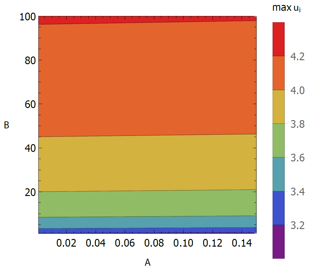
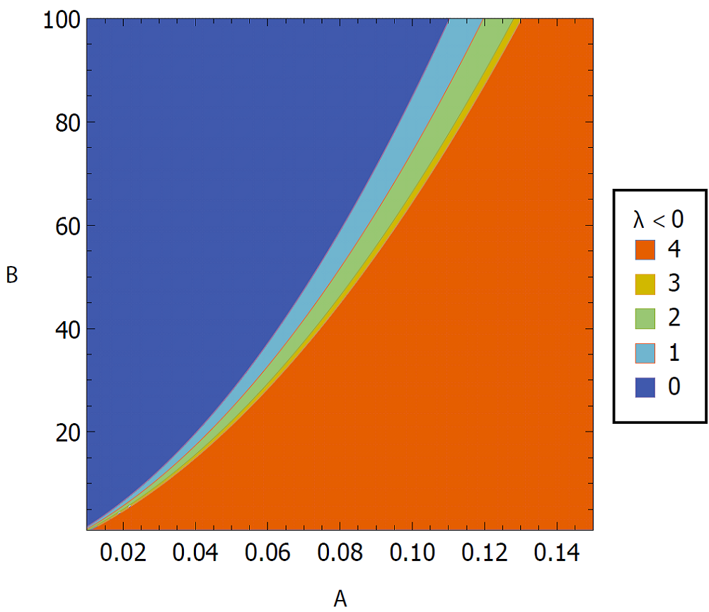
Figure 2: Left (2a): Half length of the collinear equilibrium for $n=6$. Right (2b): The number of negative eigenvalues of the Hessian.

Using Newton’s method, we have numerically computed the global collinear symmetric minimizer. The half length of the collinear equilibrium, which is equal to $2.5$ when $A=B=0$, is presented in Figure 2a for $n=6$ and different parameters.

The matrix $M_{0}$ has $1$ zero-eigenvalue. We have numerically computed that $M_{0}$ has $5$ positive eigenvalues for any $A\in[0,1]$ and $B\in[0,100]$. Therefore, the collinear equilibrium has $5$ bifurcating branches of collinear even periodic solutions.

Two of the six eigenvalues of $M_{1}$ are $0$. In Figure 2b we present the number of negative eigenvalues of $M_{1}$. The collinear equilibrium is stable in the region with zero negative eigenvalues shown in Figure 2b. In this region, there are $4$ branches of non-collinear even periodic solutions, with orbits resembling figure eights. The number of these solutions changes to $3$ in the region with $1$ negative eigenvalue in Figure 2b, to $2$ in the region with $2$ negative eigenvalues, and so on.

4.2 Circular chain

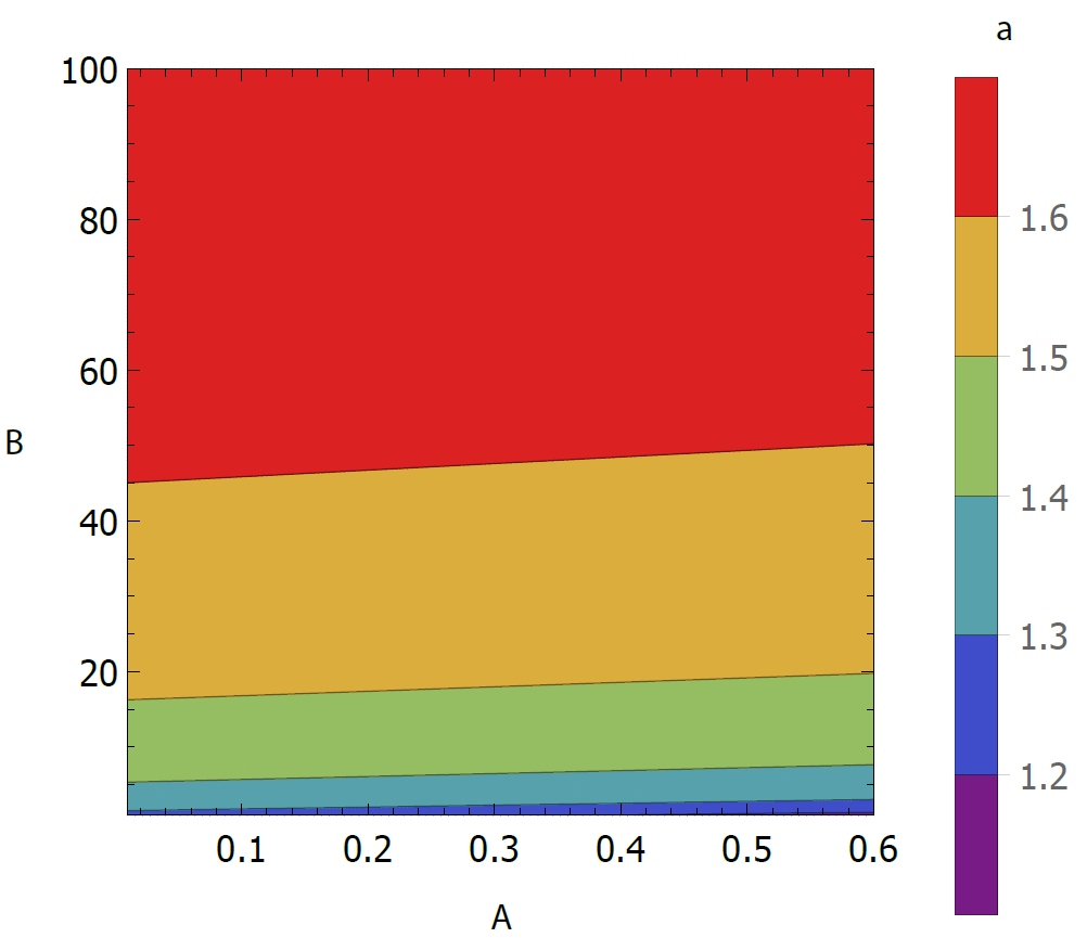
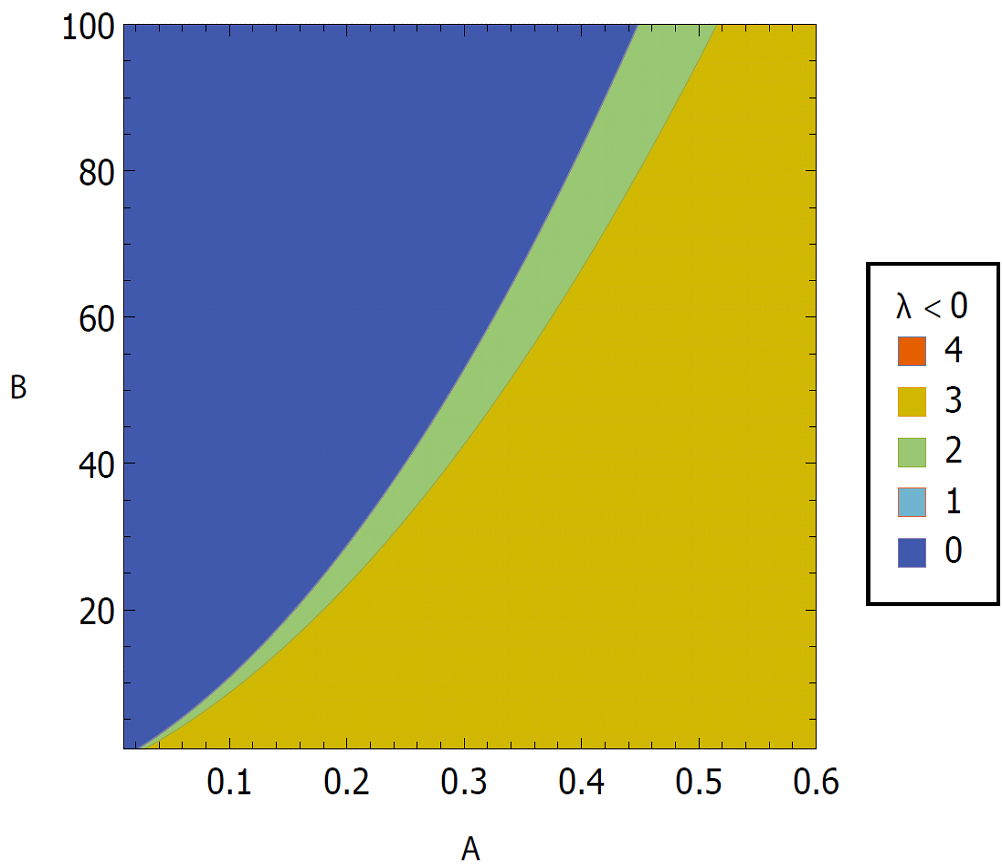
Figure 3: Left (3a): Amplitude of the circular equilibrium for $n=6$. Right (3b): Number of negative eigenvalues of the Hessian counted with multiplicity .

For $n=6$, we present the amplitude of the global minimizer among all ring configurations in Figure 3a, which is equal to $1$ when $A=B=0$. In this case, the matrix $D^{2}V(a)$ has a total of $12$ eigenvalue: $3$ are zero, $3$ are simple and $3$ are double. The circular equilibrium is stable in the region with zero negative eigenvalues shown in Figure 3a. In this region there are $3+3$ branches of periodic brake orbits. In addition, there are branches of periodic solutions of the form $x_{j}(t)=e^{jJ\zeta}x_{n}(t+jk\zeta)$.

One double eigenvalue is negative in the region with two negative eigenvalues in Figure 3b and other simple eigenvalue is negative in the region with three negative eigenvalues. This means that the circular equilibrium is unstable in these regions.

5 Conclusion

This paper is our first attempt to mathematically study stability and vibrations of configurations of atoms. We have found collinear and circular equilibria, and from them, we have proven the existence of periodic brake orbits.

Carbon atoms arrange in large chains known as alkanes and cycloalkanes. Our results confirm that cycloalkanes (ring like arrangements) are stable for $n=3$ to $8$. On the other side, we have shown that collinear arrangements are unstable from $n=3$ to $11$; these results might explain why alkanes form snake like structures instead.

With some work, our treatment can be extend to more complex structures such as fullerenes. In the future, we will present a full study of other symmetric arrangements, like the $C_{60}$ fullerene.

References

- [1] Z. Balanov, W. Krawcewicz, S. Rybicki, H. Steinlein. A short treatise on the equivariant degree theory and its applications. J. Fixed Point Theory Appl. 8 (2010) 1–74.
- [2] T. Bartsch. Topological methods for variational problems with symmetries. Lecture Notes in Mathematics 1560, Springer-Verlag, 1993.
- [3] R. Best, X. Zhu, J. Shim, P. Lopes, J. Mittal, M. Feig, A. D. Mackerell. Optimization of the Additive CHARMM All-Atom Protein Force Field Targeting Improved Sampling of the Backbone phi, psi and Side-Chain chi(1) and chi(2) Dihedral Angles. J. Chem. Theory Comput. 8 (2012) 3257–3273.
- [4] C. García-Azpeitia, J. Ize. Global bifurcation of polygonal relative equilibria for masses, vortices and dNLS oscillators. J. Differential Equations 254 (2013) 2033–2075.
- [5] C. García-Azpeitia, J. Ize. Global bifurcation of planar and spatial periodic solutions from the polygonal relative equilibria for the -body problem. J. Differential Equations 252 (2012) 5662–5678.
- [6] C. García-Azpeitia, J. Ize. Bifurcation of periodic solutions from a ring configuration of discrete nonlinear oscillators. DCDS-S 6 (2013) 975 - 983.
- [7] M. Golubitsky, D. Schaeffer. Singularities and groups in bifurcation theory II, Appl. Math. Sci. 51. Springer-Verlag, 1986.
- [8] J. Ize, A. Vignoli. Equivariant degree theory, De Gruyter Series in Nonlinear Analysis and Applications 8, Walter de Gruyter, Berlin, 2003.
- [9] L. Nirenberg. Topics in Nonlinear Functional Analysis. Courant Lecture Notes in Mathematics 6, American Mathematical Society, 2001.
- [10] F. Martínez-Farías, P. Panayotaros, A. Olvera. Weakly nonlinear localization for a 1-D FPU chain with clustering zones. Eur. Phys. J. Special Topics 223 (2014) 2943–2952.
- [11] J. Montaldi, R. Roberts. Relative Equilibria of Molecules. J. Nonlinear Sci. 9 (1999) 53–88.
- [12] L. Monticelli, D. Tieleman. Force fields for classical molecular dynamics. Methods Mol Biol. 924 (2013) 197-213.
- [13] R. Moeckel, R. Montgomery, A. Venturelli. From Brake to Syzygy. Archive for Rational Mechanics and Analysis 204 (2012) 1009–1060.
- [14] R. Palais. The principle of symmetric criticality. Commun. Math. Phys. 69 (1979) 19–30.
- [15] P. Lopes, O. Guvench, A. MacKerell. Current Status of Protein Force Fields for Molecular Dynamics Simulations. Molecular Modeling of Protein, Methods in Molecular Biology 1215 (2014) 47-71.
- [16] P. Rabinowitz, Some global results for nonlinear eigenvalue problems, J. Funct. Anal. 7 (1971) 487-513.
- [17] A. Vanderbauwhede. Local bifurcation and symmetry. Research notes in mathematics 75, Pitman Advanced Publishing Program, 1982.