Discriminative Subnetworks with Regularized Spectral Learning for Global-state Network Data

Abstract

Data mining practitioners are facing challenges from data with network structure. In this paper, we address a specific class of global-state networks which comprises of a set of network instances sharing a similar structure yet having different values at local nodes. Each instance is associated with a global state which indicates the occurrence of an event. The objective is to uncover a small set of discriminative subnetworks that can optimally classify global network values. Unlike most existing studies which explore an exponential subnetwork space, we address this difficult problem by adopting a space transformation approach. Specifically, we present an algorithm that optimizes a constrained dual-objective function to learn a low-dimensional subspace that is capable of discriminating networks labelled by different global states, while reconciling with common network topology sharing across instances. Our algorithm takes an appealing approach from spectral graph learning and we show that the globally optimum solution can be achieved via matrix eigen-decomposition.

1 Introduction

With the increasing advances in hardware and software technologies for data collection and management, practitioners in data mining are now confronted with more challenges from the collected datasets: the data are no longer as simple as objects with flattened representation but now embedded with relationships among variables describing the objects. This sort of data is often referred to as network or graph data. In the literature, there are a large number of techniques developed to mine useful patterns from network databases, ranging from frequent (sub)networks mining [15], network classification/clustering [1, 18] to anomaly detection [2]. Often, even for the same data mining task, we may need different algorithms to be developed depending on whether the networks are directed or indirected, or whether the data resides at nodes, edges or both of them [15].

In this work, the focus is on a specific class of interesting networks in which we have a series of network instances that share a common structure but may have different dynamic values at local nodes and/or edges. In addition, each network instance is associated with a global state indicating the occurrence of an event. Such a class of global-state network data can be used to model a number of real-world applications ranging from opinion evolution in social networks [20], regulatory networks in biology [21] to brain networks in neuroscience [10]. For example, we possess the same set of genes (nodes) embedded in regulatory networks. Yet, research in systems biology shows that the gene expression levels (node values) may vary across individuals and for some specific genes, their over-expressions may impact those in the neighbors through the regulatory network. These local effects may jointly encode a logical function that determines the occurrence of a disease [21, 25]. In analyzing these types of network data, a natural question to be asked is how one can learn a function that can determine the global-state values of the networks based on the dynamic values captured at their local nodes along with the network topology? More specifically, is it possible to identify a small succinct set of influential discriminative subnetworks whose local-node values have the maximum impact on the global states and thus uncover the complex relationships between local entities and the global-state network properties? In searching for an answer, obviously, a naive approach would be to enumerate all possible subnetworks and seek those who have the most discriminative potential. Nonetheless, as the number of subnetworks is exponentially proportional to the numbers of nodes and edges, this approach generally is analytically intractable and might not be feasible for large scale networks. A more practical approach is to perform heuristic sampling from the space of subnetworks. Though greatly reducing the number of subnetworks to be visited, the sampling approaches might still suffer from suboptimal solutions and might further lose explanation capability due to the large number of generating subnetworks.

In this paper, we propose a novel algorithm for mining a set of concise subnetworks whose local-state node values discriminate networks of different global-state values. Unlike the existing techniques that directly search through the exponential space of subnetworks, our proposed method is fundamentally different by investigating the discriminative subnetworks in a low dimensional transformed subspace. Toward this goal, we construct on top of the network database three meta-graphs to learn the network neighboring relationships. The first meta-graph is built to capture the network topology sharing across network instances which serves as the network constraint in our subspace learning function, whereas the two subsequent ones are build to essentially capture the relationships between neighboring networks, especially those located close to the potential discriminative boundary. By this setting, our algorithm aims to discover a unique low dimensional subspace to which: i) networks sharing similar global state values are mapped close to each other while those having different global values are mapped far apart; ii) the common network topology is smoothly preserved through constraints on the learning process. In this way, our algorithm helps to attack two challenging issues at the same time. It first avoids searching through the original space of exponential number of subnetworks by learning a single subspace via the optimization of a single dual-objective function. Second, our network topology constraint not only matches properly with our subspace learning function, its quadratic form naturally imposes the $L_{2}$-norm shrinkage over the connecting nodes, resulting in an effective selection of relevant and dominated nodes for the subnetworks embedded in the induced subspace. Additionally, the principal technical contributions of our work is the formulation of our learning objective function that is mathematically founded on spectral learning and its advantages therefore not only ensure the stability but also the global optimum of the uncovered solutions.

In summary, we claim the following contributions: (i) Novelty: We formulate the problem of mining discriminative subnetworks by transformed subspace learning—an approach that is fundamentally different from most existing techniques that address the problem in the original high-dimensional network space. (ii) Flexibility: We propose a novel dual-objective function along with constraints to ensure learning of a single subspace in which different global state networks are well discriminated while smoothly retaining their common topology. (iii) Optimality: We develop a mathematically sound solution to solve the constrained optimization problem and show that the optimal solution can be achieved via matrix eigen-decomposition. (iv) Practical relevance: We evaluate the performance of the proposed technique on both synthetic and real world datasets and demonstrate its appealing performance against related techniques in the literature.

2 Preliminaries and Problem Setting

In this section, we first introduce some preliminaries related to network data with global state values and then give the definition of our problem on mining discriminative subgraphs to distinguish global state networks.

Definition 1

(Network data instance) Given $V_{i}=\{v_{1},v_{2},\ldots,v_{n_{i}}\}$ as a set of nodes and $E_{i}\subseteq V_{i}\times V_{i}$ as a set of edges, each connecting two nodes $(v_{p},v_{q})$ if they are known to relate or influence each other, we define a network instance (or snapshot) $N_{i}$ as a quadruple $N_{i}=(V_{i},E_{i},L_{i},S_{i})$ in which $L_{i}$ is a function operating on the local states of nodes $L_{i}:V_{i}\rightarrow\mathbb{R}$ and $S_{i}$ encodes the global network state of $N_{i}$.

We consider $N_{i}$ as an indirected network and values at its local nodes are numerical (both continuous and binary) while its global state is a discrete value. Since each $N_{i}$ is associated with $S_{i}$ as its state property, $N_{i}$ is often referred to as a global-state network. For example, in the gene expression data, each $N_{i}$ corresponds to a subject and a local state indicates the gene expression level at node $v_{p}\in V_{i}$ whereas the global state encodes the presence or absence of the disease, i.e., $S_{i}\in\{presence,absence\}$. Likewise in a dynamic social network, a value at each node $v_{p}$ may encode the political standpoint of an individual whereas the global state indicates the overall political viewpoint of the entire community at some specific time (snapshot). Both local and global states may change across different network snapshots. Note that, for network instances/snapshots with different structures, we may use the null value to denote the state of a missing node and consequently, an edge in a network instance is valid only if it connects two non-null nodes.

Now, let us consider a database consisting $m$ network instances $\mathbb{N}=\{N_{1},N_{2},\ldots,N_{m}\}$, we further define the following network over these network instances:

Definition 2

(Generalized network - first meta-graph)

We define the generalized network $N$ as a triple $N=(V,E,K)$ where $V=V_{1}\cup V_{2}\ldots\cup V_{m}$ and if $\exists(v_{p},v_{q})\in E_{i}$, such an edge also exists in $E$. For a valid edge $E(p,q)\in E$, we associate a weight $K(p,q)$ as the fraction of network instances having edge $E(p,q)$ in their topology structure,i.e., $K(p,q)=m^{-1}\times\sum_{i}E_{i}(p,q)$ with $E_{i}(p,q)=1$ if there exists an edge between $v_{p}$, $v_{q}$ in network $N_{i}$. As such, $K(p,q)$ is naturally normalized between $(0,1]$. The value of 1 means the corresponding edge exists in all $N_{i}$’s while a value close to 0 shows that the edge only exists in a small fraction of network data.

It should be noted here that while we have no edge values at
individual networks $N_{i}$’s, we have non-zero value associated with each existing edge $E(p,q)$ in the generalized network $N$. Indeed, the corresponding $K(p,q)$ reflects how frequently there is an edge between $v_{p}$ and $v_{q}$ or equivalently, how strongly is the mutual influence between two entities $v_{p}$ and $v_{q}$ across all networks. As $N$ is defined based on all network instances, we also view $N$ as our first meta-graph with $V$ being its vertices and $K$ capturing its graph topology generalized from the network topology of all network instances. We are now ready to define our problem as follows.

Definition 3

(Mining Discriminative Subnetworks Problem)

Given a database of network data instances/snapshots $\mathbb{N}=\{N_{1},N_{2},\ldots,N_{m}\}$, we aim to learn an optimal and succinct set of subnetworks with respect to the topology structure generalized in the first meta-graph that well discriminate network instances with different global state values.

3 Our approach

3.1 Meta-Graphs over Network Instances

As mentioned in the above sections, searching for optimal subnetworks in the fully high dimensional original network space is always challenging and potentially intractable. We adopt an indirect yet more viable approach by transforming the original space into a low dimensional space of which networks with different global-states are well distinguished while concurrently retaining the generalized network topology captured by our first meta-graph. Toward this goal, we develop two neighboring meta-graphs based on both the local state values and global state values.

We denote these two meta-graphs respectively by $G^{+}$ and $G^{-}$. Their vertices correspond to the network instances while a link connecting two vertices represents the neighboring relationship between two corresponding network instances. For the meta-graph $G^{+}$, we denote $\mathbf{A}^{+}$ as its affinity matrix that captures the similarity of neighboring networks having the same global state values. Likewise, we denote $\mathbf{A}^{-}$ as the affinity matrix for meta-graph $G^{-}$ that captures the similarity of neighboring networks yet having different global network states. As such, $\mathbf{A}^{+}$ and $\mathbf{A}^{-}$ respectively encode the weights on the vertex-links of two corresponding graphs $G^{+}$ and $G^{-}$. In computing values for these affinity matrices, with each given network instance $N_{i}$, we find its $k$ nearest neighboring networks based on the local state values and divide them into two sets, those sharing similar global state values and those having different global states. More specifically, let $k$NN($N_{i}$) be the neighboring set of $N_{i}$, then elements of $\mathbf{A}^{+}$ and $\mathbf{A}^{-}$ are computed as: $\mathbf{A}^{+}_{ij}=\frac{\mathbf{v}_{i}\cdot\mathbf{v}_{j}}{\|\mathbf{v}_{i}\|\|\mathbf{v}_{j}\|}$ if $S_{i}=S_{j}$ and $N_{j}\in k$NN($N_{i}$) or $N_{i}\in k$NN($N_{j}$), otherwise we set $\mathbf{A}^{+}_{ij}=0$. And $\mathbf{A}^{-}_{ij}=\frac{\mathbf{v}_{i}\cdot\mathbf{v}_{j}}{\|\mathbf{v}_{i}\|\|\mathbf{v}_{j}\|}$ if $S_{i}\neq S_{j}$ and $N_{j}\in k$NN($N_{i}$) or $N_{i}\in k$NN($N_{j}$), otherwise $\mathbf{A}^{-}_{ij}=0$. In these equations, we have denoted the boldface letters $\mathbf{v}_{i}$ and $\mathbf{v}_{j}$ as the vectors encoding the dynamic local states of $N_{i}$’s and $N_{j}$’s nodes, and have used the cosine distance to define the similarity between two network instances. It is worth mentioning that, though existing other measures for network data [27], our using of cosine distance is motivated by the observation that we can view each node as a single feature and thus the network data can be essentially considered as a special case of very high dimensional data. As such, the symmetric cosine measure can be effectively used though obviously the other ones [27] can also be directly applied here.

It is also important to give the intuition behind our above computation. First, notice that both $\mathbf{A}^{+}$ and $\mathbf{A}^{-}$ are the affinity matrices having the same size of $m\times m$ since we calculate for every network instance. Second, while $\mathbf{A}^{+}$ captures the similarity of network instances sharing the same global states and neighboring to each other, $\mathbf{A}^{-}$ encodes the similarity of different global state networks yet also neighboring to each other. Such networks are likely to locate close to the discriminative boundary function and thus they play essential roles in our subsequent learning function. Third, both $\mathbf{A}^{+}$ and $\mathbf{A}^{-}$ are sparse and symmetric matrices since only $k$ neighbors are involved in computing for each network and if $N_{j}$ is neighboring to $N_{i}$, we also consider the inverse relation, i.e., $N_{i}$ is neighboring to $N_{j}$. Moreover, $\mathbf{A}^{-}$ is generally sparser compared to $\mathbf{A}^{+}$ as the immediate observation from the second remark.

3.2 Constrained Dual-Objective Function

Let us recall that $\mathbf{v}_{i}$ is the vector encoding the node states of the corresponding network $N_{i}$ and let us denote the transformation function that maps $\mathbf{v}_{i}$ into our novel target subspace by $f(\textbf{v}_{i})$. We first formulate the two objective functions as follows:

$$\operatorname*{arg\,min}_{f}\sum_{i=1}^{m}\sum_{j=1}^{m}(f(\textbf{v}_{i})-f(\textbf{v}_{j}))^{2}\mathbf{A}^{+}_{ij}$$ (1)

$$\operatorname*{arg\,max}_{f}\sum_{i=1}^{m}\sum_{j=1}^{m}(f(\textbf{v}_{i})-f(\textbf{v}_{j}))^{2}\mathbf{A}^{-}_{ij}$$ (2)

To gain more insights into these setting objectives, let us take a closer look at the first Eq.(1). If two network instances $N_{i}$ and $N_{j}$ have similar local states in the original space (i.e., $\mathbf{A}^{+}_{ij}$ is large), this first objective function will be penalized if the respective points $f(\textbf{v}_{i})$ and $f(\textbf{v}_{j})$ are mapped far part in the transformed space. As such, minimizing this cost function is equivalent to maximizing the similarity amongst instances having the same global network states in the reduced dimensional subspace. On the other hand, looking at Eq.(2) can tell us that the function will incur a high penalty (proportional to $\mathbf{A}^{-}_{ij}$) if two networks having different global states are mapped close in the induced subspace. Thus, maximizing this function is equivalent to minimizing the similarity among neighboring networks having different global states in the novel reduced subspace. As mentioned earlier, such networks tend to locate close to the discriminative boundary function and hence, maximizing the second objective function leads to the maximal margin among clusters of different global-state networks.

Having the mapping function $f(.)$ to be optimized above, it is crucial to ask which is an appropriate form for it. Either a linear or non-linear function can be selected as long as it effectively optimizes two objectives concurrently. Nonetheless, keeping in mind that our ultimate goal is to derive a set of succinct discriminative subnetworks along with their explicit nodes. Optimizing a non-linear function is generally not only more complex but importantly may lose the capability in explaining how the new features have been derived (since they will be the non-linear combinations of the original nodes). We therefore would prefer $f(.)$ as in the form of a linear combination function and following this, $f(.)$ can be represented explicitly as a transformation matrix $U_{n\times d}$ that linearly combines $n$ nodes into $d$ novel features ($d\ll n$) of the induced subspace. For the sake of discussion, we elaborate here for the projection onto 1-dimensional subspace (i.e., $d=1$). The solution for the general case $d>1$ will be straightforward once we obtain the solution for this base case. Given this simplification and with little algebra, we recast our first objective function as follows:

$$\operatorname*{arg\,min}_{\mathbf{u}} \sum_{i=1}^{m}\sum_{j=1}^{m}\|\mathbf{u}^{T}\mathbf{v}_{i}-\mathbf{u}^{T}\mathbf{v}_{j}\|^{2}\mathbf{A}^{+}_{ij}=\sum_{i=1}^{m}\sum_{j=1}^{m}tr\left(\mathbf{u}^{T}(\mathbf{v}_{i}-\mathbf{v}_{j})(\mathbf{v}_{i}-\mathbf{v}_{j})^{T}\mathbf{u}\right)\mathbf{A}^{+}_{ij}$$

$$=tr\left(\sum_{i=1}^{m}\sum_{j=1}^{m}\left(\mathbf{u}^{T}(\mathbf{v}_{i}-\mathbf{v}_{j})\mathbf{A}^{+}_{ij}(\mathbf{v}_{i}-\mathbf{v}_{j})^{T}\right)\mathbf{u}\right)$$

$$=2tr\left(\mathbf{u}^{T}\mathbf{V}\mathbf{D}^{+}\mathbf{V}^{T}\mathbf{u}\right)-2tr\left(\mathbf{u}^{T}\mathbf{V}\mathbf{A}^{+}\mathbf{V}^{T}\mathbf{u}\right)=2tr\left(\mathbf{u}^{T}\mathbf{V}\mathbf{L}^{+}\mathbf{V}^{T}\mathbf{u}\right)$$ (3)

in which we have used $tr(.)$ to denote the trace of a matrix and $\mathbf{V}$ as the matrix whose column $i$th accommodates the dynamic local states of network instance $N_{i}$ (i.e., $\mathbf{v}_{i}$), forming its size of $n\times m$. Also, $\mathbf{D}$ is the diagonal matrix whose $\mathbf{D}^{+}_{ii}=\sum_{j}\mathbf{A}^{+}_{ij}$ and we have defined $\mathbf{L}^{+}=\mathbf{D}^{+}-\mathbf{A}^{+}$, which can be shown to be the Laplacian matrix [12]. For the second objective function in Eq.(2), we can repeat the same computation which yields to the following form:

$$\operatorname*{arg\,max}_{\textbf{u}} \sum_{i=1}^{m}\sum_{j=1}^{m}\|\mathbf{u}^{T}\mathbf{v}_{i}-\mathbf{u}^{T}\mathbf{v}_{j}\|^{2}\mathbf{A}^{-}_{ij}$$

$$=2tr\left(\mathbf{u}^{T}\mathbf{V}\mathbf{D}^{-}\mathbf{V}^{T}\mathbf{u}\right)-2tr\left(\mathbf{u}^{T}\mathbf{V}\mathbf{A}^{-}\mathbf{V}^{T}\mathbf{u}\right)$$

$$=2tr\left(\mathbf{u}^{T}\mathbf{V}\mathbf{L}^{-}\mathbf{V}^{T}\mathbf{u}\right)$$ (4)

where again $\mathbf{D}^{-}$ is the diagonal matrix with $\mathbf{D}^{-}_{ii}=\sum_{j}\mathbf{A}^{-}_{ij}$ and we have defined $\mathbf{L}^{-}=\mathbf{D}^{-}-\mathbf{A}^{-}$.

Notice that while the above formulations aim at discriminating different global state networks in the low dimensional subspace, it has not yet taken into consideration the generalized network structure captured by our first meta-graph. As described previously, the mutual interactions among nodes are also important in determining the global network states. Also according to Definition 2, the larger the value placing on the link between nodes $v_{p}$ and $v_{q}$, the more likely they are being involved in the same process. Therefore, we would expect our mapping vector u not only separating well different global state networks but also ensuring its smoothness property w.r.t. the generalized network topology characterized by the first meta-graph $N$.

Toward the above objective, we formulate the network topology as a constraint in our learning objective function, and in order to be consistent with the approach based on spectral graph analysis, we encode the topology captured in $N$ by an $n\times n$ constraint matrix $\mathbf{C}$ whose elements are defined by:

$$\mathbf{C}_{pq}=\mathbf{C}_{qp}=\begin{cases}\sum_{q}K{(p,q)}&\text{if $v_{p}\equiv v_{q}$ }\\ -K(p,q)&\text{if $v_{p}$ and $v_{q}$ are connected}\\ 0&\text{otherwise }\end{cases}$$ (5)

It is easy to show that, by this definition, $\mathbf{C}$ is also the Laplacian matrix and its quadratic form, taking $\mathbf{u}$ as the vector, is always non-negative:

$$\mathbf{u}^{T}\mathbf{C}\mathbf{u} =\sum_{p=1}^{n}u_{p}^{2}\sum_{q=1}^{n}K(p,q)-\sum_{p=1}^{n}\sum_{q=1}^{n}u_{p}u_{q}K(p,q)$$

$$=\frac{1}{2}\sum_{p=1}^{n}\sum_{q=1}^{n}K(p,q)(u_{p}-u_{q})^{2}\geq 0$$ (6)

in which $u_{p},~{}u_{q}$ are components of vector $\mathbf{u}$. It is possible to observe that if $K(p,q)$ is large, indicating nodes $v_{p}$ and $v_{q}$ are strongly interacted in large portion of the network instances, the coefficients of $u_{p}$ and $u_{q}$ should be similar (i.e., smooth) in order to minimize this equation. From the network-structure perspective, we would say that if $v_{p}$ is known as a node affecting the global network state, its selection in the transformed space will increase the possibility of being selected of its nearby connected node $v_{q}$ if $K(p,q)$ is large, leading to the formation of discriminative subnetworks in the induced subspace. Therefore, in combination with the dual-objective function formulated above, we finally claim our constrained optimization problem as follows (the constants can be omitted due to optimization):

$$\mathbf{u}^{*}= \underset{\mathbf{u}}{\operatorname{arg\,max~{}}}\left\{tr\left(\mathbf{u^{T}V(L^{-}-L^{+})V}^{T}\mathbf{u}\right)\right\}$$

$$\text{~{}~{}subject to~{}~{}}\mathbf{u}^{T}\mathbf{Cu}\leq t$$

$$\text{~{}~{}~{}~{}~{}~{}~{}~{}and ~{}~{}}\mathbf{u}^{T}\mathbf{V}\mathbf{D}^{+}\mathbf{V}^{T}\mathbf{u}=1$$ (7)

The first network topology constraint aims to retain the smoothness property of $\mathbf{u}$ whereas the second constraint aims to remove its freedom, meaning that we need $\mathbf{u}$’s direction rather than its magnitude. The network topology constraint is beneficial in two ways. First as presented above, it offers a convenient and natural way to incorporate the network topology into our space transformation learning process. Second, as being formulated in the vector quadratic form, it essentially imposes the features/nodes selection through the coefficients of $\mathbf{u}$ by shrinking those of irrelevant nodes toward zero while crediting large values to those of relevant nodes. Indeed, this quadratic $L_{2}$-norm is a kind of regularization which is often referred to as the ridge shrinkage in statistics for regression [13, 7]. The parameter $t$ is used to control the amount of shrinkage. The smaller the value of $t$, the larger the amount of shrinkage.

3.3 Solving the Function

In order to solve our dual objective function associated with constraints, we resort the Lagrange multipliers method and following this, Eq. (3.2) can be rephrased as follows:

$$\mathcal{L}(\mathbf{u},\lambda)= \mathbf{u}^{T}\left(\mathbf{V\widetilde{L}V}^{T}-\alpha\mathbf{C}\right)\mathbf{u}-\lambda\left(\mathbf{u^{T}VDV^{T}u}-1\right)$$ (8)

of which, to simplify notations, we have denoted $\mathbf{\widetilde{L}=L^{-}-L^{+}}$, $\mathbf{D}=\mathbf{D}^{+}$ and $\alpha$ is used in replacement for $t$ as there is a one-to-one correspondence between them [13]. Taking the derivative of $\mathcal{L}(\mathbf{u},\lambda)$ with respect to vector $\mathbf{u}$ yields:

$$\frac{\partial\mathcal{L}(\mathbf{u},\lambda)}{\partial\mathbf{u}}=2\left(\mathbf{V\widetilde{L}V}^{T}-\alpha\mathbf{C}\right)\mathbf{u}-2\lambda\mathbf{VDV^{T}u}$$ (9)

And equating it to zero leads to the generalized eigenvalue problem:

$$\left(\mathbf{V\widetilde{L}V}^{T}-\alpha\mathbf{C}\right)\mathbf{u}=\lambda\mathbf{VDV^{T}u}$$ (10)

It is noticed that $\mathbf{V}$ is a singular matrix and its rank is at most $\min(n,m)$, making the combined matrix on the right hand side not directly invertible. We therefore decompose $\mathbf{VD}^{1/2}$ into $\mathbf{P\Sigma Q}^{T}$, where columns in $\mathbf{P}$ and $\mathbf{Q}$ are respectively called the left and right (orthonormal) singular vector of $\mathbf{VD}^{1/2}$ while $\mathbf{\Sigma}$ stores its singular values. Note that this decomposition is always possible since $\mathbf{D}$ is a non-negative diagonal matrix of node degrees. Additionally, both $\mathbf{P}$ and $\mathbf{Q}$ can be represented in the square matrices while $\mathbf{\Sigma}$ a rectangular one of $n\times m$ size according to the most general decomposition form in [6]. Following this, the combined matrix on the right hand size can be rewritten as:

$$\mathbf{VDV}^{T}=\mathbf{P\Sigma}^{2}\mathbf{P}^{T}$$ (11)

And in order to get a stable solution, we keep the top ranked singular values in $\mathbf{\Sigma}$ such as their summation explains for no less than 95% of the total singular values. Let us denote $\mathbf{B^{\ast}}=\mathbf{P\Sigma}^{-2}\mathbf{P}^{T}$ as the inversion of the right hand side and before showing our optimal solution, we need the following proposition:

Proposition 1

Let $\mathbf{P}$ be the matrix of left singular vectors of $\mathbf{VD^{1/2}}$ defined above, then its row vectors are also orthogonal, i.e., $\mathbf{P}\mathbf{P}^{T}=\mathbf{I}$

Proof

Let $\mathbf{a}$ be an arbitrary vector, we need to show $\mathbf{P}\mathbf{P}^{T}\mathbf{a}=\mathbf{a}$. Due to the orthogonal property of left singular vectors, it is true that $\mathbf{P}^{T}\mathbf{P}=\mathbf{I}$. The inversion of $\mathbf{P}$ therefore is equal to $\mathbf{P}^{T}$ and given arbitrary vector $\mathbf{a}$, there is a uniquely determined vector $\mathbf{b}$ such that $\mathbf{P}\mathbf{b}=\mathbf{a}$. Consequently,

$$\mathbf{P}\mathbf{P}^{T}\mathbf{a}=\mathbf{PP^{T}P}\mathbf{b}=\mathbf{P}\mathbf{b}=\mathbf{a}$$

It follows that $\mathbf{P}\mathbf{P}^{T}=\mathbf{I}$ since $\mathbf{a}$ is an arbitrary vector.

Theorem 3.1

Given $\mathbf{B}=\mathbf{P\Sigma}^{2}\mathbf{P}^{T}$, we have $\mathbf{BB}^{\ast}=\mathbf{I}$

Proof

The proof of this theorem is straightforward given Proposition 1.

Now, for simplicity, let us denote $\mathbf{A}$ for the combined matrix $(\mathbf{V\widetilde{L}V}^{T}-\alpha\mathbf{C})$, then it is straightforward to see that $\mathbf{u}$ turns out to be the eigenvector of the equation:

$$\mathbf{B^{\ast}A}=\lambda\mathbf{u}$$ (12)

with the maximum value is given by the following theorem.

Theorem 3.2

Given matrix $\mathbf{A}=\mathbf{V\widetilde{L}V}^{T}-\alpha\mathbf{C}$ and $\mathbf{B}=\mathbf{VDV}^{T}$ defined above, the maximum value of $\mathbf{u}^{T}\mathbf{Au}$ subjected to $\mathbf{u}^{T}\mathbf{Bu}=1$ is the largest eigenvalue of $\mathbf{B^{\ast}A}$.

Proof

Due to Theorem 3.1, it is straightforward to see that:

$$\mathbf{u}^{T}\mathbf{Au}=\mathbf{u}^{T}\mathbf{BB^{\ast}Au}$$

On the other hand, $\mathbf{u}^{T}\mathbf{BB^{\ast}Au}=\mathbf{u}^{T}\mathbf{B}\lambda\mathbf{u}$ by equation Eq. (12) and further taking into account our second constraint, it follows that:

$$\max_{\mathbf{u}:\mathbf{u}^{T}\mathbf{Bu}=1}\{\mathbf{u}^{T}\mathbf{Au}\}=\max\{\lambda\}$$

From this theorem, it is safe to say that $\mathbf{u}^{*}=\mathbf{u}_{1}$ as the first eigenvector of $\mathbf{B^{\ast}A}$ corresponding to its largest eigenvalue $\lambda_{1}$ is our optimal solution. Since eigenvectors and eigenvalues go in pair, the second optimal solution is the second eigenvector $\mathbf{u}_{2}$ corresponding to the second largest eigenvalue $\lambda_{2}$ and so on. Consequently, in the general case, if $d$ is the number of unique global network states, our optimal transformed space is the one spanned by the top $d$ eigenvectors. In the next section, we present a method to select optimal features/nodes along with the subnetworks formed by these nodes.

3.4 Subnetwork Selection

In essence, our top $d$ eigenvectors play the role of space transformation which projects network data from the original high dimensional space into the induced subspace of $d$ dimensions. Their coefficients essentially reflect how the original nodes (features) have been combined or more specifically, the degree of node’s importance in contributing to the subspace that optimally discriminates network instances. Following the approach adopted in [8] with $c$ as the user parameter, we select top $c$ entries in each $\{\mathbf{u}_{i}\}_{i=1}^{d}$ corresponding to the selective nodes. Nonetheless, it is possible that there will be more than $c$ nodes selected by combining from $d$ eigenvectors. Therefore, in practice, we may use a simple approach by first selecting the largest absolute entries across $d$ eigenvectors:

$$\mathbf{v}=\{v_{1},\ldots,v_{n}\}\text{ where }v_{p}=\ \operatorname*{max}_{i}|u_{i,p}|$$ (13)

where $u_{i,p}$ is the $p$-th entry of eigenvector $\mathbf{u}_{i}$, and then selecting nodes according to the top $c$ ranking entries in $\mathbf{v}$. The subnetworks forming from these nodes can be straightforwardly obtained by matching to the nodes in our generalized network $N$ defined in Definition 2, along with their connecting edges stored in $E$. These subnetworks can be visualized which offers the user an intuitive way to examine the results.

3.5 Computational Complexity

We name our algorithm SNL, an acronym stands for SubNetwork spectral Learning. Its computation complexity is analyzed as follows. We first need to compute edges’ weights according to Definition 2 to build our first meta-graph which takes $O(n^{2}m)$ since there are at most $n(n-1)/2$ edges in the generalized network $N$. Second, in building the two subsequent meta-graphs, the cosine distance between any two network instances is computed which amounts to $O(n^{2}m)$ or $O(mn\log n)$ in case the multidimensional binary search tree is used [3]. Also, since the size of matrix $\mathbf{VD}^{1/2}$ is $m\times n$, its singular value decomposition takes $O(mn\log n)$ with the Lanczos technique [12]. Likewise, the eigen-decomposition of the matrix $\mathbf{B^{\ast}A}$ takes $O(n^{2}\log n)$ since its size is $n\times n$. Therefore, in combination, the overall complexity is at most $O(n^{2}m+n^{2}\log n)$ assuming that the number of nodes is larger than the number of network instances.

4 Empirical Studies

4.1 Datasets and Experimental Setup

We compare the performance of SNL against MINDS [25] which is among the first approaches formally addressing the global-state network classification problem by a subnetwork sampling. Another algorithm for comparison is the Network Guided Forests (NGF) [11] designed specifically for protein protein interaction (PPI) networks. We use both synthetic and real world datasets for experimentation. Since global states are available in all datasets, we compare average accuracy in $10$-fold cross validation for synthetic data, and $5$-fold cross validation for real data (due to smaller numbers of network instances). For SNL, the cross validation is further used to select its optimal $\alpha$ parameter (shortly discussed below). Unless otherwise indicated, we set $k=10$ and use the linear-SVM to perform training and testing in the transformed space (keeping top 50 nodes) in SNL. We set MINDS’ parameters as follows: $10000$ sampling iterations, $0.8$ discriminative potential threshold and $K=200$ as recommended in the original paper [25]. The Gini index is used for the tree building in NGF and we set its improvement threshold $\epsilon=0.02$ [11].

4.2 Results on Synthetic Datasets

We use synthetic data to evaluate the performance of our technique in training robust classifiers and selecting relevant subnetworks. We generate scale-free backbone networks by preferential attachment of a predefined size adding $20$ edges for each new node. The probabilities of backbone edges are sampled from a truncated Gaussian distributions: $N(0.9,0.1)$ for edges among ground truth nodes (pre-selected nodes of high-correlation with the network state) and $N(0.7,0.1)$ for the rest of the edges. The weighted backbone serves as our generalized template to generate network instances by independently sampling the existence of every edge based on its probability. The global states are binary $S_{i}\in\{0,1\}$ with balanced distribution. We further add noise to both global and local states of ground truth nodes, respectively with levels of $10\%$ and $30\%$.

Varying $|V_{gt}|$:

In the first set of experiments, we aim to test whether the performance of all algorithms is affected by the number of ground truth nodes. To this end, we generate 5 datasets by fixing $m=1000$ instances, $n=3000$ nodes and vary the ground truth nodes $|V_{gt}|$ from 10 to 50. In Figure 2, we report the average accuracy (and standard deviation) of all algorithms in 10-fold cross validation. As one may observe, SNL performs stably regardless of the change in the ground truth sizes. Compared to the other techniques, its classification is always consistently higher across all cases. The MINDS technique also performs well on this experimental setting yet the NGF seems to be sensitive to the small ground truth sizes. For small $|V_{gt}|$, the sampling strategy based on density areas employed in NGF has little chance to select the ground truth nodes, making its accuracy close to a random technique. When more ground truth nodes are introduced, NGF has higher possibility to sample high-utility nodes and in the last two datasets, its performance is on par with that of MINDS. Nonetheless, its accuracy only peaks at 73% in the best case which is lower than 77% in SNL (last column).

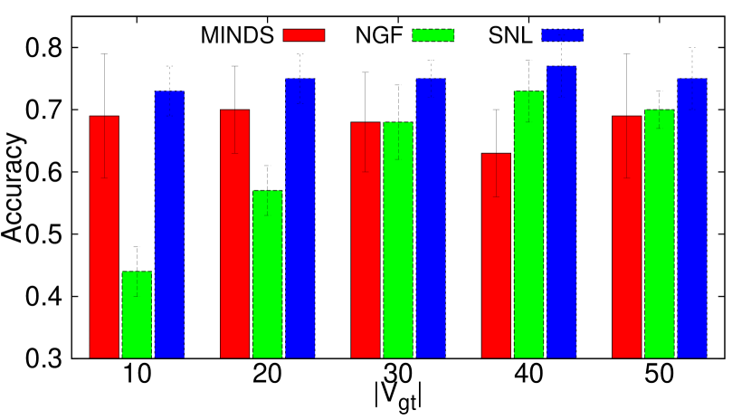
Figure 1: Accuracy of all algorithms by varying ground truth subnetworks’ nodes

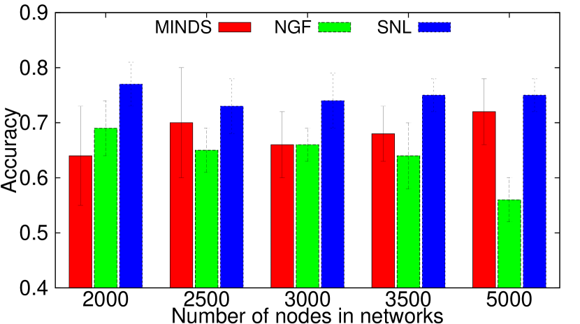
Figure 2: Accuracy of all algorithms by varying network size

Varying network size:

In the second set of experiments, we evaluate the performance of all algorithms by varying the network sizes. Specifically, we fix $m=3000$ network instances, $|V_{gt}|=50$ ground truth nodes and generate 5 datasets having the network size varied from 2000 to 5000 nodes. The classification performance along with the standard deviation is reported in Figure 2. It is possible to see that the performance traits are similar to those in our first set of experiments. SNL’s classification accuracy remains high while that of NGF decreases with the increase of network size. This again can be explained by the extension of the searching subnetwork space, leading to the lower likelihood of both NGF and MINDS in identifying relevant subnetworks with potentially discriminative nodes. The slightly better performance of MINDS (compared to NGF) is due to its accuracy thresholding in selecting candidate substructures. The set of MINDS’ selected trees are thus qualitatively better. Nonetheless, as compared to SNL, our subspace learning approach show more competitive results. Moreover, since the low-dimensional subspace learnt in SNL is unique and linearly combined from the most discriminative nodes, its performance also shows more stable, indicated by the small standard deviation across all cases.

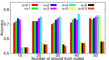
Figure 3: Network effect on accuracy 3 and AUC performance 3 for different numbers of ground truth nodes.

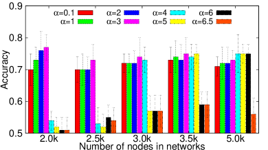
Figure 4: Network effect on accuracy 3 and AUC 3 for different network sizes.

Effect of network topology:

In order to provide more insights into the performance of SNL, we further test the network effect. As presented in Section 3, $\alpha$ is the parameter controlling the influence of the network information on the subspace learning process. The higher the $\alpha$, the more preference putting on the heavily connected nodes. We report in Figures 3,4 the accuracy of SNL by varying $\alpha$ from $0.1$ to $6.5$ and in Figures 3,4 its ability in discovering the ground truth nodes. For the latter case, we validate the performance through the usage of area under the ROC curve (AUC) [13].

As expected, incorporating the network structure in the subspace learning process improves both classification rate and the AUC in uncovering the ground truth nodes. The plots in Figures 3,4 show that the accuracy initially improves for increasing influence of the network ($\alpha\leq 5$) and then decreases as the network component becomes prevalently dominant ($\alpha>5$). This is because for large $\alpha$, SNL tends to incorporate irrelevant nodes solely based on their strong connections to the neighbors (yet their local values might not help classifying global state values). Another notable observation is that, in larger instances or ground truth feature sets, the optimal $\alpha$ tends to increase as well. Moreover, the values of $\alpha$ that maximize classification accuracy also result in optimal AUC in identifying the ground truth nodes (Fig. 3,4). These experiments clearly show the helpful information provided by the network topology in uncovering the groundtruth features. Also, we exclude NGF and MINDS from these experiments (to save space) and leave the discussion over their AUC performance with the real-world datasets.

4.3 Real-world Datasets

We use $4$ real-world datasets to evaluate the performance of SNL and its competing methods. The features in all datasets correspond to micro-array expression measurements of genes; the topology structures relating features correspond to gene interaction networks; and the global network states correspond to phenotypic traits of the subjects/instances. The statistics of our datasets are listed in Table 1. Two of our real-world datasets, breast cancer and embryonic development, were also used for experimentation in the original NGF method  [11]. Our other datasets come from a study on maize properties [14] and a human liver metastasis study [19] combined with a functional network [9]. The network samples are used as provided in the original studies, except for maize where we down-sample one of the classes to balance the global state distribution.

Table 1: Real-world dataset statistics and sources

Datasets	Genes	Edges	Instances	Global State
Breast cancer	$11203$	$57235$	$295$	cancer/non-cancer
Embryonic development	$1321$	$5227$	$35$	developmental tissue layer
Maize	$8574$	$298510$	$344$	high/low oil production
Liver metastasis	$7383$	$251916$	$123$	disease/non-disease

Classification performance:

The comparison of classification accuracy for all techniques and datasets is presented in Figure 5. We report the average accuracy and standard deviation from the 5-fold stratified cross validation. All techniques perform competitively on the breast cancer data, achieving more than 70% of classification accuracy on average. The accuracy of SNL dominates significantly that of the sampling techniques on the embryonic and maize datasets (at least $15\%$ and $10\%$ improvement respectively) and less so in the liver dataset. The separation is highest in the datasets of small number of instances and big number of feature nodes – the settings in which SNL is particularly effective. Beyond average performance improvement, SNL’s accuracy is also more stable across all folds as it considers the global network structure when learning a subspace for classification, while the alternatives perform sampling in the exponential space of substructures.

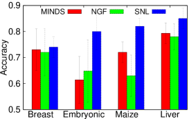
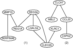
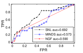
Figure 5: 5 Classification performance of all algorithms on four real world datasets. 5 Subnetworks identified by the SNL related to the liver metastasis. 5 ROC performance over the liver metastasis ($x$-axis is false positive rate, $y$-axis is true positive rate).

Subnetwork discovery:

Unlike the synthetic datasets where we can control the ground truth network features, it is generally much harder to obtain ground truth subnetworks for real world datasets. However, as an attempt to look deeper into the results, we choose the Liver metastasis and further investigate the meaningful subnetworks generated by the SNL. For this dataset, out of top 50 nodes of highest coefficient values (ref. Section 3.4), about one third of the nodes are connected into four subnetworks. We depict in Figure 5 the two largest ones which respectively contain 7 and 4 connected gene nodes. Among these selected subnetworks, the genes REG1A and REG3A are particularly interesting since they are in agreement with the ones found in [19] which was shown to be involved in the liver metastasis cancer. As a comparison against MINDS and NGF, we notice that both methods generate multiple binary-trees where each node has only a single parent. Moreover, while SNL can provide a natural rank of important genes based on their coefficients (from the learnt subspace), it is less trivial to define important genes from NGF and MINDS as they both generate thousands of trees. For the purpose of measuring biological relevance of obtained genes, we define a ranking for these competing techniques based on the frequency of genes appeared in the generated trees. For comparison, we select $46$ metastasis-specific genes identified in [19] to serve as a ground truth set (39 intersect with our network and expression data) and plot the ROC performance of all algorithms in Figure 5. Note that, this is only a partial ground truth set, since identifying all genes associated with this disease is a subject of ongoing research [19]. It is observed that the ranking produced by SNL includes more ground truth genes than those of NGF and MINDS at increasing false-positive rates. The higher true positive rates of SNL makes it a better method for identifying new genes associated with the phenotype of interest. In practice, this is an important feature of the algorithm since validating even a single gene related to cancer is both time-wise and financially costly. As shown in Figure 5, while the ROC performance of NGF and MINDS are only at $0.59$ and $0.57$ AUC, that value of SNL is $0.69$ which clearly demonstrates large gap of better performance.

5 Related Work

Mining discriminative subspaces from global-state networks is a novel and challenging problem. Two lines of work close to this problem are network classification and mining evolving subgraphs from dynamic network data. In the network classification case, most representative algorithms are LEAP [28], graphSig [26], GAIA [17] and COM [16] which generally assume a database consisting of positive and negative networks that need to be classified. These approaches, though diverse in terms of their underlying algorithms, all aim at extracting a set significant subnetworks that are more frequent in one class of positive networks and less frequent in the negative class. Different from the above problems, we aim to mine subnetworks which are represented in all network instances; yet the node values along with the network structures can discriminate the global states of the networks. Another line of related research focuses on mining dynamic evolving subnetworks [23, 4, 5]. The problem in this case is to obtain subnetworks over time that evolve significantly (outliers) from other network locations. This setting therefore do not model the problem developed in this paper since the dynamic network snapshots neither contain global-state values nor can remove their temporal property.

Several studies in systems biology have indicated the critical role of the network structure in identifying protein modules related to clinical outcomes, for both regression [22, 24, 21] and classification [11, 25]. In the classification setting which is related to our study, the NGF [11] is an ensemble approach that builds a forest of trees jointly voting for the class of a network instance. Resided at the NGF’s core is the CART (classification and Regression tree) technique and in order to build a decision tree within the PPI network, NGF starts with a root node and progressively includes connected nodes as long as the improvement in class separation (measured by Gini index) is no smaller than a given threshold. The study in [25] is the first one to formally introduce the problem of subnetwork mining in global-state networks and further propose the MINDS algorithm to solve it. Similar to NGF, MINDS adopts network-constraint decision trees and is also an ensemble classifier. Nonetheless, it increases the quality of decision trees by developing a novel concept of editing map over the space of potential subnetworks and exploits Monte Carlo Markov Chain sampling over this novel data structure to seek decision trees with maximum classification potential. Unlike the frequency-based and sampling classification discussed above, our approach is fundamentally different as it searches for the most discriminative subnetworks in a single low dimensional subspace through the spectral learning technique, which generally leads to more stable and high-accuracy performance.

6 Conclusion

We proposed a novel algorithm named SNL to address the challenging problem of uncovering the relationship between local state values residing on nodes and the global network events. While most existing studies address this problem by sampling the exponential subnetworks space, we adopt an efficient and effective subspace transformation approach. Specifically, we define three meta-graphs to capture the essential neighboring relationships among network instances and devise a spectral graph theory algorithm to learn an optimal subspace in which networks with different global-states are well separated while the common structure across samples is smoothly respected to enable subnetwork discovery. Through experimental analysis on synthetic data and real-world datasets, we demonstrated its appealing performance in both classification accuracy and the real-world relevance of the discovered discriminative subnetwork features.

Acknowledgements: The research work was supported in part by the NSF (IIS-1219254) and the NIH (R21-GM094649).

References

- [1] C. C. Aggarwal and H. Wang. A survey of clustering algorithms for graph data. In Managing and Mining Graph Data, pages 275–301. 2010.
- [2] L. Akoglu, M. McGlohon, and C. Faloutsos. oddball: Spotting anomalies in weighted graphs. In PAKDD (2), pages 410–421, 2010.
- [3] J. L. Bentley. Multidimensional binary search trees used for associative searching. 18(9):509–517, 1975.
- [4] P. Bogdanov, C. Faloutsos, M. Mongiovì, E. E. Papalexakis, R. Ranca, and A. K. Singh. Netspot: Spotting significant anomalous regions on dynamic networks. In SDM, pages 28–36, 2013.
- [5] P. Bogdanov, M. Mongiovì, and A. K. Singh. Mining heavy subgraphs in time-evolving networks. In ICDM, pages 81–90, 2011.
- [6] A. K. Cline and I. S. Dhillon. Computation of the Singular Value Decomposition. Handbook of Linear Algebra, CRC Press, 2006.
- [7] X. H. Dang, I. Assent, R. T. Ng, A. Zimek, and E. Schubert. Discriminative features for identifying and interpreting outliers. In ICDE, pages 88–99, 2014.
- [8] X. H. Dang, B. Micenková, I. Assent, and R. T. Ng. Local outlier detection with interpretation. In ECML/PKDD (3), pages 304–320, 2013.
- [9] R. Dannenfelser, N. R. Clark, and A. Ma’ayan. Genes2fans: connecting genes through functional association networks. BMC bioinformatics, 13(1):156, 2012.
- [10] I. N. Davidson, S. Gilpin, O. T. Carmichael, and P. B. Walker. Network discovery via constrained tensor analysis of fmri data. In KDD, pages 194–202, 2013.
- [11] J. Dutkowski and T. Ideker. Protein networks as logic functions in development and cancer. PLoS Computational Biology, 7(9), 2011.
- [12] G. H. Golub and C. F. V. Loan. Matrix Computations. The Johns Hopkins University Press, 3rd edition, 1996.
- [13] T. Hastie, R. Tibshirani, and J. Friedman. The Elements of Statistical Learning. Data Mining, Inference, and Prediction. 2001.
- [14] L. Hui, P. Zhiyu, et al. Genome-wide association study dissects the genetic architecture of oil biosynthesis in maize kernels. Nature Genetics, 45:43–50, 2013.
- [15] C. Jiang, F. Coenen, and M. Zito. A survey of frequent subgraph mining algorithms. Knowledge Eng. Review, 28(1):75–105, 2013.
- [16] N. Jin, C. Young, and W. Wang. Graph classification based on pattern co-occurrence. In CIKM, pages 573–582, 2009.
- [17] N. Jin, C. Young, and W. Wang. Gaia: graph classification using evolutionary computation. In SIGMOD Conference, pages 879–890, 2010.
- [18] N. S. Ketkar, L. B. Holder, and D. J. Cook. Empirical comparison of graph classification algorithms. In ICDM, pages 259–266, 2009.
- [19] D. H. Ki, H.-C. Jeung, C. H. Park, S. H. Kang, G. Y. Lee, W. S. Lee, N. K. Kim, H. C. Chung, and S. Y. Rha. Whole genome analysis for liver metastasis gene signatures in colorectal cancer. Int J Cancer, 121(9):2005–2012, 2007.
- [20] D. Lee, O.-R. Jeong, and S.-g. Lee. Opinion mining of customer feedback data on the web. ICUIMC ’08, pages 230–235. ACM, 2008.
- [21] C. Li and H. Li. Network-constrained regularization and variable selection for analysis of genomic data. Bioinformatics, 24(9):1175–1182, 2008.
- [22] C. Li and H. Li. Variable selection and regression analysis for graph-structured covariates with an application to genomics. The Annals of Applied Statistics, 4(3):1498–1516, 2010.
- [23] M. Mongiovì, P. Bogdanov, and A. K. Singh. Mining evolving network processes. In ICDM, pages 537–546, 2013.
- [24] J. Noirel, G. Sanguinetti, and P. C. Wright. Identifying differentially expressed subnetworks with mmg. Bioinformatics, 24(23):2792–2793, 2008.
- [25] S. Ranu, M. Hoang, and A. K. Singh. Mining discriminative subgraphs from global-state networks. In KDD, pages 509–517, 2013.
- [26] S. Ranu and A. K. Singh. Graphsig: A scalable approach to mining significant subgraphs in large graph databases. In ICDE, pages 844–855, 2009.
- [27] S. Soundarajan, T. Eliassi-Rad, and B. Gallagher. Which network similarity method should you choose? In Workshop on Information Networks at NYU, 2013.
- [28] X. Yan, H. Cheng, J. Han, and P. S. Yu. Mining significant graph patterns by leap search. In SIGMOD Conference, pages 433–444, 2008.