Regularized Estimation of Piecewise Constant Gaussian Graphical Models: The Group-Fused Graphical Lasso

Abstract

The time-evolving precision matrix of a piecewise-constant Gaussian graphical model encodes the dynamic conditional dependency structure of a multivariate time-series. Traditionally, graphical models are estimated under the assumption that data is drawn identically from a generating distribution. Introducing sparsity and sparse-difference inducing priors we relax these assumptions and propose a novel regularized M-estimator to jointly estimate both the graph and changepoint structure. The resulting estimator possesses the ability to therefore favor sparse dependency structures and/or smoothly evolving graph structures, as required. Moreover, our approach extends current methods to allow estimation of changepoints that are grouped across multiple dependencies in a system. An efficient algorithm for estimating structure is proposed. We study the empirical recovery properties in a synthetic setting. The qualitative effect of grouped changepoint estimation is then demonstrated by applying the method on a genetic time-course data-set.

Keywords: Changepoint; High-dimensional; M-estimator; Sparsity; Time-series;

1 Introduction

High-dimensional correlated time series are found in many modern socio-scientific domains such as neurology, cyber-security, genetics and economics. A multivariate approach, where the system is modeled jointly, can potentially reveal important inter-dependencies between variables. However, naive approaches which permit arbitrary (graphical) dependency structures and dynamics are infeasible because the number of possible graphs becomes exponentially large as the number of variables increases.

For data streams with continuous-valued variables, a penalized maximum likelihood approach offers a flexible means to estimate the underlying dependency structure and continues to attract much attention. In this setting a common assumption is that the data is drawn from a multivariate distribution where the conditional dependency structure is in some sense sparse— the dependency graph is expected to constitute a small proportion of the total number of possible edges. Typically, a Gaussian likelihood is accompanied by a sparsity inducing prior. For example, Banerjee et al. (2008) and Friedman et al. (2008) penalize the likelihood with an $\ell_{1}$ norm applied to the precision matrix (non-convex penalties have also been investigated, see Chun et al. (2014)). Further extensions have been considered, for example Lafferty et al. (2012) who graphical model estimation in the non-parametric case, and more recently Lee and Hastie (2015) study models with mixed types of variable.

It is of particular interest to understand how dependency graphs evolve over time, and how prior knowledge relating to such dynamics can be exploited to constrain the graph estimation. Specifically, we consider how a piecewise constant graphical model can be estimated such that the dependency graphs are constant in locally stationary regions segmented by a set of changepoints. This is a challenging problem. If the changepoints were known in advance then local graph estimation could be performed. However, the changepoints cannot be found without first estimating the graphs. Previous approaches (Angelosante and Giannakis, 2011) have resorted to using dynamic programming alongside the $\ell_{1}$ graph learning approaches. Unfortunately, these are restricted to quadratic computational complexity as a function of the time-series length. An alternative approach as followed by Ahmed and Xing (2009); Kolar and Xing (2012) and others is to formulate a convex optimization problem with suitable constraints that encourage desired dynamical properties. We refer to such approaches as fused graphical models.

Our contribution investigates and extends a class of models to enable the estimation of changepoints that are grouped over multiple edges in a graphical model. Such grouped changepoints indicate changes in dependency across a system that influence many variables at once. In many situations there may be a priori knowledge of potential groups (for example, grouping over different gene function in genetic data or asset classes in finance). Grouped changes often indicate some sort of regime or phase change in the system dynamics which may be of interest to the practitioner. To this end we propose the group-fused graphical lasso (GFGL) method for joint changepoint and graph estimation. We contrast the proposed grouped estimation of changepoints in graphical models with previous approaches which enforce changepoints at the level of individual edges only and which therefore fail to capture such grouping behavior.

In Section 2, we describe current dynamical graphical model estimation; we introduce our main contribution in the form of the GFGL estimator; and contrast this with previously proposed fused graphical model approaches. Following this, in Section 3 we present an efficient alternating-directed method of moments (ADMM) algorithm for estimation with GFGL. The proposed methodology is demonstrated on simulated examples in Section 4, before we consider an application looking at temporal-evolution of gene dependencies in Section 5. We conclude with a discussion of the work. Some technical details are summarized in the Appendix which can be found in the on-line supplementary material.

2 Dynamic Gaussian Graphical Models

Given a $P$-variate time-series $\boldsymbol{y}^{t}\sim\mathcal{N}(\boldsymbol{\mu}^{t},\boldsymbol{\Sigma}^{t})$ for $t=1,\ldots,T$, if the precision matrices $\boldsymbol{\Theta}^{t}:=(\boldsymbol{\Sigma}^{t})^{-1}$ are well defined then the dependency structure of the series can be captured by a dynamic Gaussian Graphical Model (GGM). This comprises a collection of graphs $G^{t}=(V^{t},E^{t})$, where the vertices $V^{t}=\{1,\ldots,P\}$ represent each component of $\boldsymbol{y}^{t}$ and the edges $E^{t}$ represent conditional dependency relations between variables over time. More precisely, the edge $(i,j)\in{E}^{t}$ is present in the graph if the $i$ and $j$th variables are conditionally dependent given all other variables. It follows in the Gaussian case that conditional independence $y_{i}^{t}\perp y_{j}^{t}|\>y_{-\{i,j\}}^{t}$ is satisfied if and only if the corresponding entries of the precision matrix are zero, i.e. $\Theta_{ij}^{t}=\Theta_{ji}^{t}=0$ (Lauritzen, 1996). Therefore, since it encodes the conditional dependency graph, estimation of the precision matrix is of great interest.

Traditionally, estimation of GGM’s is performed under the assumption of stationarity, i.e. we have identically distributed draws from a Gaussian model. Letting $\boldsymbol{Y}=(\boldsymbol{y}^{1},\ldots,\boldsymbol{y}^{T})$ be a set of observations and assuming $\boldsymbol{y}^{t}\,{\buildrel{\rm iid}\over{\sim}}\,\mathcal{N}(\boldsymbol{0},\boldsymbol{\Sigma})$, one can construct an estimator for $\boldsymbol{\Sigma}^{-1}$ by maximizing the log-likelihood: $\hat{\boldsymbol{\Theta}}:={\arg\max}_{\boldsymbol{X}}\big{[}\mathrm{log}\big{(}\mathrm{det}(\boldsymbol{X})\big{)}-\mathrm{tr}(\hat{\boldsymbol{S}}\boldsymbol{X})\big{]}$, where $\hat{\boldsymbol{S}}=\boldsymbol{Y}\boldsymbol{Y}^{\top}/2T$. In the case where the number of observations is greater than the number of variables ($T>P$) we can test for edge significance to find a GGM (Drton and Perlman, 2004). However, in the non-identical case, because only one data-point may be observed at each node per time-step the traditional empirical covariance estimator $\hat{\boldsymbol{S}}^{t}=\boldsymbol{y}^{t}(\boldsymbol{y}^{t})^{\top}/2$ is rank deficient for $P>1$. To this end, estimation of the precision matrix requires additional modeling assumptions. A strategy explored in several recent works (Ahmed and Xing, 2009; Danaher et al., 2013; Gibberd and Nelson, 2014; Monti et al., 2014) is to introduce priors in the form of regularized M-estimators, viz.

$$\hat{\boldsymbol{\Theta}}^{t}:=\underset{\boldsymbol{X}^{t}\in\{\boldsymbol{X}_{+}^{t}\}_{t=1}^{T}}{\arg\min}\big{[}\mathcal{L}(\{\boldsymbol{X}^{t}\})\big{]},$$ (1)

with a convex cost function:

$$\mathcal{L}(\{\boldsymbol{X}^{t}\})=\sum_{t=1}^{T}-L(\boldsymbol{X}^{t},\boldsymbol{y}^{t})+R_{\mathrm{Shrink}}(\{\boldsymbol{X}^{t}\})+R_{\mathrm{Smooth}}(\{\boldsymbol{X}^{t}\})\;,$$ (2)

where $L(\boldsymbol{X}^{t},\boldsymbol{y}^{t})$ is proportional to the log-likelihood and follows from the normal distribution. The penalty terms $R_{\mathrm{Shrink}}$, $R_{\mathrm{Smooth}}$ correspond to prior shrinkage/smoothness assumptions. Typically, the smoothness term will be a function of the difference between estimates $\boldsymbol{X}^{t}-\boldsymbol{X}^{t-1}$, whereas the shrinkage term will act at specific time points, i.e. directly on $\boldsymbol{X}^{t}$.

One popular approach that is relevant to GGM is to use these regularizers to place assumptions on the number of dependencies in a graph. For example, in the i.i.d. case, we need not consider conditional dependencies between all variables, but only a small subset of those which appear most dependent. This assumption of sparsity can be viewed as placing a prior on the parameters $\boldsymbol{\Theta}$ to induce zeros in the off-diagonal entries of the precision matrix. Akin to the Laplace prior associated with the least absolute shrinkage and selection operator (lasso) for linear regression (Tibshirani, 1996), one can construct the graphical lasso estimator for the precision matrix as: $\hat{\boldsymbol{\Theta}}:=\arg\min_{\boldsymbol{X}}\big{[}-L(\boldsymbol{X},\hat{\boldsymbol{S}})+\lambda\|\boldsymbol{X}\|_{1}\big{]}$, where $L(\boldsymbol{X},\hat{\boldsymbol{S}})=\mathrm{log}\big{(}\mathrm{det}(\boldsymbol{X})\big{)}-\mathrm{tr}(\hat{\boldsymbol{S}}\boldsymbol{X})$. This estimator, as examined by Banerjee et al. (2007); Friedman et al. (2008) allows one to stabilize estimation of the precision matrix in the high-dimensional regime (where $P>T$) and estimate a sparse graph $\hat{G}$ (sparsity is controlled by $\lambda$). A full Bayesian treatment for the graphical lasso is given by Wang (2012) who investigate how representative the mode is of the full posterior.

Several approaches which incorporate dynamics in such graphical estimators have been suggested. Zhou et al. (2010); Kolar and Xing (2011) utilize a local estimate of the covariance in the term $L(\boldsymbol{X}^{t})$ by replacing $\hat{\boldsymbol{S}}$ in the graphical lasso with a time-sensitive weighted estimator

$$\hat{\boldsymbol{S}}^{t}=\sum_{s}w_{s}^{t}\boldsymbol{y}_{s}(\boldsymbol{y}_{s})^{\top}/\sum_{s}w_{s}^{t}\,,$$ (3)

where $w_{s}^{t}=K(|s-t|/h)$ are weights derived from a symmetric non-negative smoothing kernel function $K(\cdot)$ with width related to $h$. The resulting graphs $\hat{G}^{t}$ are now representative of some temporally localized data. By making some smoothness assumptions on the underlying covariance matrix such a kernel estimator can be shown to be risk consistent (Zhou et al., 2010). Kolar and Xing (2011) go further, and demonstrate that placing assumptions on the Fisher information matrix allows one to prove consistent estimation of graph structure in such dynamic GGM. In the next section we discuss how one may adapt these assumptions to estimate piecewise constant GGM.

2.1 The group fused graphical lasso

We propose the Group Fused Graphical Lasso (GFGL) estimator for estimating piecewise constant GGM. The model assumes data is generated at time-point $t=1,\ldots,T$ according to $\mathbb{R}^{P}\ni\boldsymbol{y}^{t}\sim\mathcal{N}(\boldsymbol{0},\boldsymbol{\Sigma}^{t})$, where the distribution is strictly stationary i.e. $\{\boldsymbol{\Sigma}^{l}=\boldsymbol{\Sigma}^{m}|\tau^{k}<l,m\leq\tau^{k+1}\}$ between $k=0,\ldots,K$ changepoints (note we set $\tau^{0}=0,\tau^{K+1}=T$). We propose to estimate the covariance and precision matrix at each time by minimizing a cost, as in Eq. (1). The GFGL cost is given as:

$$\mathcal{L}(\{\boldsymbol{X}^{t}\})={\displaystyle\underset{\propto\mathrm{-Likelihood}}{\underbrace{\sum_{t=1}^{T}\overset{-L(\{\boldsymbol{X}^{t}\},\{\boldsymbol{y}^{t}\})}{\overbrace{\big{(}-\mathrm{log}\mathrm{det}(\boldsymbol{X}^{t})+\mathrm{tr}(\hat{\boldsymbol{S}}^{t}\boldsymbol{X}^{t})\big{)}}}}}}\underset{\mathrm{\ell_{1}\;\mathrm{shrinkage}}}{+\underbrace{\overset{R_{\mathrm{Shrink}}}{\overbrace{\lambda_{1}\sum_{t=1}^{T}\|\boldsymbol{X}_{-ii}^{t}\|_{1}}}}}+\underset{\mathrm{group\>\ell_{2,1}\>smoothing}}{\underbrace{\overset{R_{\mathrm{Smooth}}}{\overbrace{\lambda_{2}{\displaystyle\sum_{t=2}^{T}}\|\boldsymbol{X}_{-ii}^{t}-\boldsymbol{X}_{-ii}^{t-1}\|_{F}}}}},$$ (4)

where $\|\boldsymbol{X}_{-ii}^{t}\|=\sum_{i\neq j}|X_{i,j}^{t}|$ is the matrix $\ell_{1}$ norm with the diagonal entries removed.

In the remainder of this paper we describe how one can efficiently solve the GFGL problem and demonstrate two key properties, namely:

1. Estimated precision matrices encode a sparse dependency structure whereby many of the off axis entries are exactly zero, i.e. $\hat{\Theta}^{t}_{i,j}=0$.

2. Precision matrices maintain a piecewise constant structure where changepoints tend to be grouped across the precision matrix, such that for many edges indexed by $(i,j)$ and $(l,m)$ the estimated changepoints for the two edges are the same, viz. $\hat{\mathcal{T}}_{i,j}=\hat{\mathcal{T}}_{l,m}$ where $\hat{\mathcal{T}}_{i,j}=\{\hat{\tau}^{1}_{ij},\ldots,\hat{\tau}^{\hat{K}_{ij}}_{ij}\}$ represents the set of $\hat{K}_{ij}$ estimated changepoints $\tau^{k}_{ij}$ on the $i,j$th edge).

2.2 Relationship to previous proposals

Name	References	Likelihood $L$	Graph Smoothing $R_{\mathrm{Smooth}}$
Dynamic Graphical Lasso	Zhou et al. (2010)	$\big{\{}\mathrm{log}\big{(}\mathrm{det}(\boldsymbol{X}^{t})\big{)}-\mathrm{tr}(\hat{\boldsymbol{S}}^{t}\boldsymbol{X}^{t})\big{\}}_{t=1}^{T}$	via kernel (see Eq. 3)
Temporally smoothed $\ell_{1}$ logistic regression (TESLA)	Ahmed and Xing (2009)	$\sum_{t=1}^{T}\big{[}\log\big{(}1+\exp(\boldsymbol{y}_{-i}^{t}X_{\cdot,i}^{t})\big{)}-\boldsymbol{y}_{-i}^{t}X_{\cdot,i}^{t}y_{i}^{t}\big{]}$	$\lambda_{2}\sum_{t=2}^{T}\|\boldsymbol{X}_{-ii}^{t}-\boldsymbol{X}_{-ii}^{t-1}\|_{1}$
Joint Graphical Lasso (JGL)*	Danaher et al. (2013)	$\sum_{k=1}^{K}\big{[}n_{k}\big{(}\mathrm{log}\big{(}\mathrm{det}(\boldsymbol{X}^{k})\big{)}-\mathrm{tr}(\hat{\boldsymbol{S}}^{k}\boldsymbol{X}^{k})\big{)}\big{]}$	$\lambda_{2}\sum_{k<k^{\prime}}\|\boldsymbol{X}^{k}-\boldsymbol{X}^{k^{\prime}}\|_{1}$
Fused Multiple Graphical Lasso (FMGL)*	Yang et al. (2015)	$\sum_{k=1}^{K}\big{[}n_{k}\big{(}\mathrm{log}\big{(}\mathrm{det}(\boldsymbol{X}^{k})\big{)}-\mathrm{tr}(\hat{\boldsymbol{S}}^{k}\boldsymbol{X}^{k})\big{)}\big{]}$	$\lambda_{2}\sum_{k=1}^{K}\|\boldsymbol{X}^{k}-\boldsymbol{X}^{k-1}\|_{1}$
SINGLE	Monti et al. (2014)	$\sum_{t=1}^{T}\big{[}\mathrm{log}\big{(}\mathrm{det}(\boldsymbol{X}^{t})\big{)}-\mathrm{tr}(\hat{\boldsymbol{S}}^{t}\boldsymbol{X}^{t})\big{]}$	$\lambda_{2}\sum_{t=2}^{T}\|\boldsymbol{X}_{-ii}^{t}-\boldsymbol{X}_{-ii}^{t-1}\|_{1}$
VCVS Model	Kolar and Xing (2012)	For each node $p=1,\ldots,P$ $\sum_{t=1}^{T}\big{(}y_{t,p}-\sum_{i\neq p}y_{t,i}\beta_{i,t}\big{)}^{2}$	$\lambda_{2}\sum_{t=1}^{T}\|\boldsymbol{\beta}_{\cdot,t}-\boldsymbol{\beta}_{\cdot,t-1}\|_{2}$
GFGL	(this work)	$\sum_{t=1}^{T}\big{[}\mathrm{log}\big{(}\mathrm{det}(\boldsymbol{X}^{t})\big{)}-\mathrm{tr}(\hat{\boldsymbol{S}}^{t}\boldsymbol{X}^{t})\big{]}$	$\lambda_{2}\sum_{t=2}^{T}\|\boldsymbol{X}_{-ii}^{t}-\boldsymbol{X}_{-ii}^{t-1}\|_{F}$

Table 1: Overview of likelihood and smoothing approaches for dynamic graphical modeling. Shrinkage via an $\ell_{1}$ term is common to all methods (in VCVS this is applied at the node-wise level) above when used for edge selection. This is usually applied to off-diagonal entries in the graph/precision matrix such that $R_{\mathrm{Shrink}}=\lambda_{1}\sum_{t=1}^{T}\|\boldsymbol{X}_{-ii}^{t}\|_{1}$. * Note: these methods are not specifically designed for time-series data but for building fused models over different $k=1,\ldots,K$ classes/experiments each with $n_{k}$ data-points.

Unlike most previous proposals (see Table 1) GFGL penalizes changes across groups of edges in the graph. One notable exception to this can be found in the Varying-Coefficient Varying-Structure (VCVS) model of Kolar and Xing (2012) who propose to select changepoints with an $\ell_{2}$ type norm over the differences. The motivation in that work is similar to ours. However, the authors formulate the graph-selection problem differently, utilizing a node-wise regularized regression estimator, rather than the multivariate Gaussian likelihood we use. Whilst node-wise estimation can recover the conditional dependency graph, it does not in general result in a valid (positive definite) precision matrix. This is in contrast to our approach here, where the positive-definite precision matrices can be used to define a probabilistic model via the GGM.

In particular we consider comparison to $\ell_{1}$ fused methods such as FMGL (Yang et al., 2015), TESLA (Ahmed and Xing, 2009), SINGLE (Monti et al., 2014) and JGL (Danaher et al., 2013). These methods are similar to each other in that they permit finding a smoothed graphical model through a fused $\ell_{1}$ term. Throughout the paper we will refer to models of this type as the Independent Fused Graphical Lasso (IFGL) with the same cost function as GFGL (see Eq. 4), but with the group-smoothing term replaced with an $\ell_{1}$ penalized difference, such that $R_{\mathrm{smooth}}=\lambda_{2}\sum_{t=2}^{T}\|\boldsymbol{X}^{t}-\boldsymbol{X}^{t-1}\|_{1}$. Rather than focusing on the smoothly evolving graph through the kernel covariance estimator $\hat{\boldsymbol{S}}^{t}$, we instead study the difference between the smoothing regularizer for IFGL and GFGL. Throughout the rest of this paper we adopt a purely piecewise constant graph model, in this setting, the empirical covariance is simply estimated with the data at time $t$ according to; $\hat{\boldsymbol{S}}^{t}=\boldsymbol{y}^{t}(\boldsymbol{y}^{t})^{\top}/2$. One can think of this as using a Dirac-delta kernel for the covariance estimate. For example in Eq. (3) we can set $w_{s}^{t}=\delta(s-t)$.

3 Algorithms for the group fused graphical lasso problem

Since the penalty function of IFGL approaches solely comprises $\ell_{1}$ terms it is linearly separable. As such this permits block-coordinate descent approaches utilized, for example, by Friedman et al. (2008); Yang et al. (2015) whereby the precision matrix rows and columns are sequentially updated. Unfortunately, the GFGL objective (Eq. 4) does not have the same linear separability structure. This is due to the norm $\|\boldsymbol{X}^{t}-\boldsymbol{X}^{t-1}\|_{F}:=(\sum_{i,j}(X_{i,j}^{t}-X_{i,j}^{t-1})^{2})^{1/2}$ acting across the whole (or at least multiple rows/columns) of the precision matrix. This lack of linear separability across the precision matrices precludes a block-coordinate descent strategy (Tseng and Yun, 2009). Instead, we make use of the separability of the group norm (with respect to time) and propose an Alternating Directed Method of Moments (ADMM) algorithm. A key innovation of our contribution is to incorporate an iterative proximal projection step to solve the Group Fused Lasso sub-problem. Additionally, we demonstrate how the same framework can be utilized to solve the previously proposed IFGL problem.

3.1 An alternating directions method of multipliers approach

The ADMM approach we adopt to optimize the GFGL objective Eq. (4) splits $\mathcal{L}(\{\boldsymbol{X}^{t}\})$ into two separate, but related problems. Equivalently to solving Eq. (1) we can solve:

$$\hat{\boldsymbol{\Theta}} = \underset{\{\boldsymbol{X}^{t},\boldsymbol{Z}^{t}\}_{t=1}^{T}}{\arg\min}\bigg{[}{\displaystyle\sum_{t=1}^{T}\big{(}-\mathrm{log}\mathrm{det}(\boldsymbol{X}^{t})+\mathrm{tr}(\boldsymbol{S}^{t}\boldsymbol{X}^{t})\big{)}}+\lambda_{1}\sum_{t=1}^{T}\|\boldsymbol{Z}_{-ii}^{t}\|_{1}+\lambda_{2}{\displaystyle\sum_{t=2}^{T}}\|\boldsymbol{Z}_{-ii}^{t}-\boldsymbol{Z}_{-ii}^{t-1}\|_{F}\bigg{]}$$ (5)

$$\mathrm{such}\;\mathrm{that}:\;\boldsymbol{X}^{t}-\boldsymbol{Z}^{t}=\boldsymbol{0}\;,$$

where $\{\boldsymbol{X}^{t}\}$ and the auxiliary variables $\{\boldsymbol{Z}^{t}\}$ are also constrained to be positive-semi-definite. The augmented Lagrangian for GFGL is given as:

$$\mathcal{L}(\{\boldsymbol{X}^{t}\},\{\boldsymbol{Z}^{t}\},\{\boldsymbol{Y}^{t}\}): = {\displaystyle\sum_{t=1}^{T}\big{(}-\mathrm{log}\mathrm{det}(\boldsymbol{X}^{t})+\mathrm{tr}(\boldsymbol{S}^{t}\boldsymbol{X}^{t})\big{)}}+\lambda_{1}\sum_{t=1}^{T}\|\boldsymbol{Z}_{-ii}^{t}\|_{1}\;\ldots$$

$$+ \lambda_{2}{\displaystyle\sum_{t=2}^{T}}\|\boldsymbol{Z}_{-ii}^{t}-\boldsymbol{Z}_{-ii}^{t-1}\|_{F}+\sum_{t=1}^{T}\langle\boldsymbol{Y}^{t},\boldsymbol{X}^{t}-\boldsymbol{Z}^{t}\rangle+\frac{\gamma}{2}\sum_{t=1}^{T}\|\boldsymbol{X}^{t}-\boldsymbol{Z}^{t}\|_{F}^{2},$$

where $\{\boldsymbol{Y}^{t}\}_{t=1}^{T}$ is a set of dual matrices $\boldsymbol{Y}^{t}\in\mathbb{R}^{P\times P}$. The difference between ADMM and the more traditional augmented Lagrangian method (ALM) (Glowinski and Le Tallec, 1989) is that we do not need to solve for $\{\boldsymbol{X}^{t}\}$ and $\{\boldsymbol{Z}^{t}\}$ jointly. Instead, we can take advantage of the separability structure highlighted in Eq. (5) to solve $\{\boldsymbol{X}^{t}\}$,$\{\boldsymbol{Z}^{t}\}$ separately. By combining the inner product terms and the augmentation term we find:

$$\mathcal{L}(\{\boldsymbol{X}^{t}\},\{\boldsymbol{Z}^{t}\},\{\boldsymbol{U}^{t}\}): = {\displaystyle\sum_{t=1}^{T}\big{(}-\mathrm{log}\mathrm{det}(\boldsymbol{X}^{t})+\mathrm{tr}(\boldsymbol{S}^{t}\boldsymbol{X}^{t})\big{)}}+\lambda_{1}\sum_{t=1}^{T}\|\boldsymbol{Z}_{-ii}^{t}\|_{1}\;\ldots$$

$$+ \lambda_{2}{\displaystyle\sum_{t=2}^{T}}\|\boldsymbol{Z}_{-ii}^{t}-\boldsymbol{Z}_{-ii}^{t-1}\|_{F}+\frac{\gamma}{2}\sum_{t=1}^{T}\big{(}\|\boldsymbol{X}^{t}-\boldsymbol{Z}^{t}+\boldsymbol{U}^{t}\|_{F}^{2}-\|\boldsymbol{U}^{t}\|_{F}^{2}\big{)},$$

where $\boldsymbol{U}^{t}=(1/\gamma)\boldsymbol{Y}^{t}$ is a rescaled dual variable. We write the solution at the $n$th iteration as $\{\boldsymbol{X}_{(n)}^{t}\}=\{\boldsymbol{X}_{(n)}^{1},\ldots\boldsymbol{X}_{(n)}^{T}\}$ and proceed by updating our estimates according to the three steps below;

1. Likelihood Update ($\mathrm{for\;}t=1,\ldots,T$):

   $$\boldsymbol{X}_{(n)}^{t} = \arg\min_{\boldsymbol{X}^{t}}\bigg{[}-\mathrm{log}\mathrm{det}(\boldsymbol{X}^{t})+\mathrm{tr}(\hat{\boldsymbol{S}}{}^{t}\boldsymbol{X}^{t})+\frac{\gamma}{2}\|\boldsymbol{X}^{t}-\boldsymbol{Z}_{(n-1)}^{t}+\boldsymbol{U}_{(n-1)}^{t}\|_{F}^{2}\bigg{]}\;,\;$$ (6)

2. Constraint Update:

   $$\{\boldsymbol{Z}_{(n)}^{t}\} = \arg\min_{\{\boldsymbol{Z}^{t}\}}\bigg{[}\frac{\gamma}{2}\sum_{t=1}^{T}\|\boldsymbol{X}_{(n)}^{t}-\boldsymbol{Z}^{t}+\boldsymbol{U}_{(n-1)}^{t}\|_{F}^{2}+\lambda_{1}\sum\|\boldsymbol{Z}_{-ii}^{t}\|_{1}\;\ldots$$ (7)

   $$\quad\quad\quad\ldots+\;\lambda_{2}\sum_{t=2}^{T}\|\boldsymbol{Z}_{-ii}^{t}-\boldsymbol{Z}_{-ii}^{t-1}\|_{F}\bigg{]}\;,$$

3. Dual Update ($\mathrm{for\;}t=1,\ldots,T$):

   $$\boldsymbol{U}_{(n)}^{t} = \boldsymbol{U}_{(n-1)}^{t}+\big{(}\boldsymbol{X}_{(n)}^{t}-\boldsymbol{Z}_{(n)}^{t}\big{)}\;.$$ (8)

3.2 Likelihood update (Step 1)

We can solve the update for $\boldsymbol{\Theta}_{(n)}^{t}$ through an eigen-decomposition of terms in the covariance, auxiliary and dual variables (Yuan, 2011; Monti et al., 2014). If we differentiate the objective in Eq. (6) and set the result equal to zero we find:

$$(\boldsymbol{X}^{t})^{-1}-\gamma\boldsymbol{X}^{t}=\hat{\boldsymbol{S}}^{t}-\gamma(\boldsymbol{Z}_{(n-1)}^{t}-\boldsymbol{U}_{(n-1)}^{t}).$$ (9)

Noting that $\boldsymbol{X}^{t}$ and $\boldsymbol{S}^{t}-\gamma(\boldsymbol{Z}_{(n-1)}^{t}-\boldsymbol{U}_{(n-1)}^{t})$ share the same eigenvectors (see Appendix for details) we can now solve for the eigenvalues of $\boldsymbol{X}^{t}$. For each eigenvalue $\{x_{h}\}_{h=1}^{P}=\mathrm{eigval}(\boldsymbol{X}^{t})$ and $\{s_{h}\}_{h=1}^{P}=\mathrm{eigval}\big{(}\hat{\boldsymbol{S}}^{t}-\gamma(\boldsymbol{Z}_{(n-1)}^{t}-\boldsymbol{U}_{(n-1)}^{t})\big{)}$ we can construct the quadratic equation $x_{h}^{-1}-\gamma x_{h}=s_{h}$. The right hand side of Eq. (9) contains evidence from the data-set via $\hat{\boldsymbol{S}}^{t}$, but also takes into account the effect our priors encoded in $\boldsymbol{Z}_{(n-1)}^{t}$, from the non-smooth portion of Eq. (5). Upon solving for $x_{h}$ given $s_{h}$ we find:

$$x_{h}=\frac{1}{2\gamma}\big{(}-s_{h}+\sqrt{s_{h}^{2}+4\gamma}\big{)}\;.$$

The full precision matrix $\boldsymbol{X}^{t}$ can now be found through the eigen-decomposition:

$$\boldsymbol{X}_{(n)}^{t}=\boldsymbol{V}\boldsymbol{Q}\boldsymbol{V}^{\top},$$

where $\boldsymbol{V}$ contains the eigenvectors of $\hat{\boldsymbol{S}}^{t}-\gamma(\boldsymbol{Z}_{(n-1)}^{t}-\boldsymbol{U}_{(n-1)}^{t})$ as columns and $\boldsymbol{Q}\in\mathbb{R}^{P\times P}$ is a diagonal matrix populated by the eigenvalues $x_{h}$, ie $Q_{hh}=x_{h}$. We note that, by choosing the positive solution for the quadratic, we ensure that $\boldsymbol{X}_{(n)}^{t}$ is positive-definite and thus produces a valid estimator for the precision matrix. Since Eq. (6) refers to an estimation at each time-point separately, we can solve for each $\boldsymbol{X}_{(n)}^{t}$ independently for $t={1,\ldots,T}$ to yield the set $\{\boldsymbol{X}_{(n)}^{t}\}_{t=1}^{T}$. Indeed this update can be computed in parallel, as appropriate.

3.3 Group fused lasso signal approximator (Step 2)

The main difference between this work and previous approaches is in the use of a grouped constraint. This becomes a significant challenge when updating $\{\boldsymbol{Z}^{t}\}$ in Eq. (7). Unlike the calculation of $\{\boldsymbol{X}_{(n)}^{t}\}$, we cannot separate the optimization over each time-step. Instead, we must solve for the whole set of matrices $\{\boldsymbol{Z}^{t}\}$ jointly. In addition, due to the grouped term in GFGL, we cannot separate the optimization across individual edges. In contrast to independent penalization strategies (Monti et al., 2014; Danaher et al., 2013) it is not possible to solve GFGL for $\{X_{ij}^{t}\}$ independently of $\{X_{kl}^{t}\}$, where $(i,j)\neq(k,l)$. Such an inconvenience is to be expected as the constraints which extract changepoints in GFGL can act across all elements in $\boldsymbol{X}^{t}$.

For notational convenience we re-write step two in vector form. Since each $\boldsymbol{Z}^{t}$ is symmetric about the diagonal we can reduce the number of elements by simply taking the elements above the diagonal $\boldsymbol{z}^{t}=(Z_{i,j}^{t}|\>\mathrm{for\>}j>i,\;i=1,\ldots,P)^{\top}$. We then construct a matrix form such that $\boldsymbol{Z}=(\boldsymbol{z}^{1},\ldots,\boldsymbol{z}^{T})^{\top}\in\mathbb{R}^{T\times P(P-1)/2}$, whereby row $t$ of the matrix correspond to values at time-step $t$. We perform similar transformations for $\boldsymbol{X}^{t}\rightarrow\boldsymbol{X}$ and $\boldsymbol{U}^{t}\rightarrow\boldsymbol{U}$, and set $\bar{\lambda}_{1}=\lambda_{1}/\gamma$ and $\bar{\lambda}_{2}=\lambda_{2}/\gamma$ . Re-writing the objective in Eq. (7) with these transformations yields the cost function

$$G(\boldsymbol{Z};\bar{\lambda_{1}},\bar{\lambda_{2}})=\underset{L(\boldsymbol{Z})}{\underbrace{\frac{1}{2}\|\boldsymbol{X}_{(n)}-\boldsymbol{Z}+\boldsymbol{U}_{(n-1)}\|_{F}^{2}}}+\underset{R_{1}(\boldsymbol{Z})}{\underbrace{\bar{\lambda}_{1}\|\boldsymbol{Z}\|_{1}}}+\underset{R_{2}(\boldsymbol{Z})}{\underbrace{\bar{\lambda}_{2}\|\boldsymbol{D}\boldsymbol{Z}\|_{2,1}}},$$ (10)

where $\boldsymbol{D}\in\mathbb{R}^{(T-1)\times T}$ is a backwards differencing matrix of the form $D_{i,i}=-1,D_{i,i+1}=-1$ for $i=1,\ldots,T-1$ and zero otherwise, the the group $\ell_{2,1}$ norm is defined as $\|\boldsymbol{X}\|_{2,1}:=\sum_{t}\|X_{t,\cdot}\|_{2}$. If one constructs a target matrix $\boldsymbol{A}=\boldsymbol{X}_{(n)}+\boldsymbol{U}_{(n-1)}$ then

$$\mathcal{Z}(\boldsymbol{A};\bar{\lambda_{1}},\bar{\lambda_{2}})=\arg\min_{\boldsymbol{Z}}G(\boldsymbol{Z};\bar{\lambda_{1}},\bar{\lambda_{2}}),$$ (11)

looks like a signal approximation problem, we will refer to this problem as the Group-Fused Lasso Signal Approximator (GFLSA). This looks similar to the previously studied Fused Lasso Signal Approximator (FLSA) (Liu et al., 2010) but crucially $R_{2}(\boldsymbol{Z})$ incorporates a group $\ell_{2,1}$ norm rather than the $\ell_{1}$ norm of FLSA.

We note Eq. (11) can also be thought of as a proximity operator, such that $\mathcal{Z}(\boldsymbol{A};\lambda_{1},\lambda_{2})\equiv\mathrm{prox}_{R_{1}+R_{2}}(\boldsymbol{A})$. If $R_{1}$ and $R_{2}$ were indicator functions of two closed convex sets $C$ and $D$ respectively, then $\mathcal{Z}(\boldsymbol{A};\lambda_{1},\lambda_{2})$ would find the best approximation to $\boldsymbol{A}$ restricted to the set $C\cap D$. Unlike FLSA which penalizes the columns of $\boldsymbol{Z}$ independently, we find $\mathrm{prox}_{R1+R2}(\boldsymbol{A})\neq\mathrm{prox}_{R2}\big{(}\mathrm{prox}_{R1}(\boldsymbol{A})\big{)}$ and cannot apply the two-stage smooth-then-sparsify theorem of Friedman et al. (2007); Liu et al. (2010). Instead, we follow the work of Alaíz et al. (2013) and adopt an iterative projection approach which utilizes Dykstra’s method (Combettes and Pesquet, 2011) to find a feasible solution for both the group fused $\ell_{2,1}$ and lasso $\ell_{1}$ constraints.

For any unconstrained optimal point $\boldsymbol{Z}^{*}=\arg\min_{\boldsymbol{Z}}L(\boldsymbol{Z})$ there exists a set of parameters $(\lambda_{1},\lambda_{2})\in[0,\infty)$ which will act to move the optimal point of the regularized case $\boldsymbol{Z}_{r}^{*}=\arg\min_{\boldsymbol{Z}}G(\boldsymbol{Z};\lambda_{1},\lambda_{2})$ such that $\boldsymbol{Z}^{*}\neq\boldsymbol{Z}_{r}^{*}$ where:

$$\boldsymbol{Z}_{r}^{*}=\underset{\boldsymbol{Z}}{\arg\min}L(\boldsymbol{Z}),\quad\text{ subject to }\quad\|\boldsymbol{Z}\|_{1}\leq l_{1}\quad\mathrm{and}\quad\sum_{t=2}^{T}\|(\boldsymbol{DZ})_{t,\cdot}\|_{2}\leq l_{2}.$$

For a given likelihood term, we can obtain an $l_{1}$ sparse and $l_{2}$ smooth solution by solving a penalized problem instead of the explicitly constrained version above. Such a penalized form is found in Eq. (10) and, while $R_{1}(\lambda_{1},\boldsymbol{Z})$ and $R_{2}(\lambda_{2},\boldsymbol{Z})$ are not explicitly indicator functions (i.e. they do not take values $\infty$ outside some feasible region), there does exist a mapping between the values of the parameters $\lambda_{1}\geq 0\>,\lambda_{2}\geq 0$ and the corresponding $l_{1},l_{2}$ sparsity and smoothness constraints. To give some intuition, for a given constraint level $l_{1}$ and function $L(\boldsymbol{Z})$, the size of the feasible set given by $C_{\lambda_{1}}=\{\boldsymbol{Z}\>|\>\lambda_{1}\|\boldsymbol{Z}\|_{1}\leq l_{1}\}$, reduces as $\lambda_{1}$ increases. Thus sparsity is a monotonically non-decreasing function of $\lambda_{1}$ The same argument can be constructed for smoothing and the constraint set $D_{\lambda_{2}}=\{\boldsymbol{Z}\>|\>\lambda_{2}\sum_{t}\|(\boldsymbol{DZ})_{t,\cdot}\|_{2}\leq l_{2}\}$. The proximal Dykstra method provides a way to calculate a point $\boldsymbol{Z}_{r}^{*}\in C_{\lambda_{1}}\cap D_{\lambda_{2}}$ that is, in the sense of the $\ell_{2}$ distance, close or proximal to the unconstrained solution for $\arg\min_{\boldsymbol{Z}}L(\boldsymbol{Z})=\boldsymbol{A}$. By iterating between the feasibility of a solution in $C_{\lambda_{1}}$ and $D_{\lambda_{2}}$ (see Algorithm 1), a solution can be found which is both suitably smooth and sparse.

Result: $\mathrm{prox}_{R_{1}+R_{2}}(\boldsymbol{A})$

$\boldsymbol{Z}_{(0)}=\boldsymbol{A}\;,\boldsymbol{U}_{(n)}=\boldsymbol{0}\;,\;\boldsymbol{Q}_{(n)}=\boldsymbol{0}$

while not converged,$\;n=0,1,\ldots$ do

       $\boldsymbol{V}_{(n)}=\mathrm{prox}_{R2}(\boldsymbol{Z}_{(n)}+\boldsymbol{U}_{(n)})$

       $\boldsymbol{U}_{(n+1)}=\boldsymbol{Z}_{(n)}+\boldsymbol{U}_{(n)}-\boldsymbol{V}_{(n)}$

       $\boldsymbol{Z}_{(n+1)}=\mathrm{prox}_{R1}(\boldsymbol{V}_{(n)}+\boldsymbol{Q}_{(n)})$

       $\boldsymbol{Q}_{(n+1)}=\boldsymbol{V}_{(n)}+\boldsymbol{Q}_{(n)}-\boldsymbol{Z}_{(n+1)}$

      

end while

Algorithm 1 Dykstras iterative projection algorithm

Given that iterative projection can be used to find a feasible point, the challenge is now to compute the separate proximity operators for $R_{1}$ and $R_{2}$. The proximal operator for the $\ell_{1}$ term $\mathrm{prox}_{R1}(\boldsymbol{A})$ is given by the soft-thresholding operator (Tibshirani, 1996):

$$\mathrm{prox}_{R1}(\boldsymbol{A};\lambda_{1}) = \underset{\boldsymbol{Z}}{\arg\min}\frac{1}{2}\|\boldsymbol{Z}-\boldsymbol{A}\|_{F}^{2}+\lambda_{1}\|\boldsymbol{Z}\|_{1}$$ (12)

$$= \mathrm{sign}(\boldsymbol{A})\odot\max(|\boldsymbol{A}|-\lambda_{1},\boldsymbol{0})\;,$$

where the $\max$ and $\mathrm{sign}$ functions act in an element-wise manner and $\odot$ denotes element-wise multiplication.

Computing the group-fused term $\mathrm{prox}_{R2}(\boldsymbol{A})$ is more involved and there is no obvious closed-form solution, instead we tackle this through a block-coordinate descent approach similar to that considered by Bleakley and Vert (2011) and Yuan and Lin (2006). Our target here is to find the proximal operator for the group smoothing aspect of the regularizer, which we write as:

$$\mathrm{prox}_{R2}(\boldsymbol{A};\lambda_{2})=\underset{\boldsymbol{Z}}{\arg\min}\frac{1}{2}\|\boldsymbol{Z}-\boldsymbol{A}\|_{F}^{2}+\lambda_{2}\|\boldsymbol{D}\boldsymbol{Z}\|_{2,1}.$$ (13)

Re-writing the above with $\boldsymbol{\Omega}=\boldsymbol{D}\boldsymbol{Z}$ and constructing $\boldsymbol{Z}$ as a sum of differences via $Z_{t,\cdot}=\boldsymbol{\omega}+\sum_{i=1}^{t-1}\Omega_{i,\cdot}$, (where $\boldsymbol{\omega}=Z_{1,\cdot}$) then one can interpret the proximal operator as a group lasso problem (Bleakley and Vert, 2011) . Writing the re-parameterized problem in matrix form one can show that solving for the jump parameters allows us to reconstruct an estimate for $\boldsymbol{Z}$. This is formally equivalent to a group lasso (Yuan and Lin, 2006) class of problem:

$$\hat{\boldsymbol{\Omega}}:=\underset{\boldsymbol{\Omega}\in\mathbb{R}^{(T-1)\times P(P-1)/2}}{\arg\min}\frac{1}{2}\|\bar{\boldsymbol{A}}-\bar{\boldsymbol{R}}\boldsymbol{\Omega}\|_{F}^{2}+\lambda_{2}\|\boldsymbol{\Omega}\|_{2,1}\;,$$ (14)

where a bar $\bar{\boldsymbol{X}}$ denotes a column centered matrix and $\boldsymbol{R}\in\mathbb{R}^{T\times(T-1)}$ is a matrix with entries $R_{i,j}=1$ for $i>j$ and $0$ otherwise. The problem above can be solved through a block-coordinate descent strategy, sequentially updating the solution for each block $\Omega_{t,\cdot}$ for $t=1,\ldots,T-1$ (see Appendix). We can then construct a solution for $\hat{\boldsymbol{Z}}$ by summing the differences and noting that the optimal value for $\boldsymbol{\omega}$ is given by $\hat{\boldsymbol{\omega}}=\boldsymbol{1}_{1,T}(\boldsymbol{A}-\boldsymbol{R}\hat{\boldsymbol{\Omega}})$. Correspondingly, the proximal operator for $R_{2}$ is found via

$$\mathrm{prox}_{R2}(\boldsymbol{A};\lambda_{2})=\big{(}\hat{\boldsymbol{\omega}}^{\top},(\hat{\boldsymbol{\omega}}+\hat{\Omega}_{1,\cdot})^{\top},\ldots,(\hat{\boldsymbol{\omega}}+\sum_{i=1}^{T-1}\hat{\Omega}_{i,\cdot})^{\top}\big{)}{}^{\top}.$$ (15)

The overall subproblem Eq. (10) can now be solved through iteratively applying the proximity operators according to Dykstra’s algorithm (Alg. 1).

3.4 Dual update and convergence (step 3)

The final step in the ADMM-based method is to update the dual variable via Eq. (8). Convergence properties of general ADMM algorithms are analyzed in Glowinski and Le Tallec (1989). The sequence of solutions $\{\boldsymbol{X}_{(n)}\}_{n\in\mathbb{N}}$ can be shown to converge (Eckstein and Bertsekas, 1992) to the solution of the problem: $\arg\min_{\boldsymbol{X}\in\mathbb{R}^{N}}\;f(\boldsymbol{X})+g(\boldsymbol{L}\boldsymbol{X})$, under conditions that $\boldsymbol{L}^{\top}\boldsymbol{L}$ is invertible and the intersection between relative interiors of domains is non-empty: $(\mathrm{ri}\>\mathrm{dom}\>g)\cap\mathrm{ri}\;\boldsymbol{L}(\mathrm{dom}\>f)\neq\emptyset$. In the GFGL and IFGL problems considered here one simply sets $\boldsymbol{L=\boldsymbol{I}}$, in order to restrict $\boldsymbol{X}=\boldsymbol{Z}$. Clearly in this case $\boldsymbol{I}^{\top}\boldsymbol{I}$ is invertible and $\mathrm{dom}\>g=\boldsymbol{I}(\mathrm{dom}\>f)$; thus the relative interiors intersect.

Whilst ADMM is guaranteed to converge to an optimal solution, in practice it converges relatively fast to a useful solution, but very slowly if high accuracy is required. Following the approach of Boyd et al. (2011) we consider tracking two convergence criteria: one tracking primal feasibility: $r_{\mathrm{prime}}=\sum_{t=1}^{T}\|\boldsymbol{X}_{(n)}^{t}-\boldsymbol{Z}_{(n)}^{t}\|_{F}^{2}\;$, relating to the optimality requirement $\boldsymbol{X}^{*}-\boldsymbol{Z}^{*}=\boldsymbol{0}$, and the other looking at dual feasibility: $r_{\mathrm{dual}}=\sum_{t=1}^{T}\|\boldsymbol{Z}_{(n)}^{t}-\boldsymbol{Z}_{(n-1)}^{t}\|_{F}^{2}\;$, which tracks the requirement that $\boldsymbol{0}\in\nabla f(\boldsymbol{X}^{*})+\boldsymbol{U}^{*}$, where ^∗ denotes optimal value. The rate at which the algorithm converges is somewhat tunable through the $\gamma$ parameter. However it is not clear how to find an optimal $\gamma$ for a given problem. In practice we find that a value of order $\gamma=10$ provides reasonably fast convergence which with tolerances order; $r_{\mathrm{prime}}<\epsilon_{\mathrm{prime}}=10^{-3}$ and $r_{\mathrm{dual}}<\epsilon_{\mathrm{dual}}=10^{-3}$.

Data: $\boldsymbol{y}^{1},\ldots,\boldsymbol{y}^{T}$

Input: $\lambda_{1},\;\lambda_{2},\;\gamma,\;\epsilon_{\mathrm{dual}},\;\epsilon_{\mathrm{prime}}$

Result: $\{\hat{\boldsymbol{\Theta}}^{1},\ldots,\hat{\boldsymbol{\Theta}}^{T}\}$

Calculate covariance matrix: $\hat{\boldsymbol{S}}^{t}=\boldsymbol{y}^{t}(\boldsymbol{y}^{t})^{\top}/2\;\mathrm{for}\;t=1,\ldots,T$

Initialize: $\boldsymbol{Z}^{t}_{(0)}=\boldsymbol{X}^{t}_{(0)}=\boldsymbol{U}^{t}_{(0)}=\boldsymbol{0}$

while not converged ($r_{\mathrm{prime}}\geq\epsilon_{\mathrm{prime}},\;r_{\mathrm{dual}}\geq\epsilon_{\mathrm{dual}}$), $\;n=0,1,\ldots$ do

       for t=1,…,T do

             Eigen-decomposition: $\{s_{h},\;\boldsymbol{v}_{h}\}_{h=1}^{P}=\mathrm{eigen}\big{(}\hat{\boldsymbol{S}}^{t}-\gamma(\boldsymbol{Z}_{(n-1)}^{t}-\boldsymbol{U}_{(n-1)}^{t})\big{)}$

             $x_{h}=\big{(}-s_{h}+\sqrt{s_{h}^{2}+4\gamma}\big{)}/2\gamma\;$

             $\boldsymbol{V}=(\boldsymbol{v}_{1},\ldots.\boldsymbol{v}_{P}),\;\boldsymbol{Q}=\mathrm{diag}(x_{1},\ldots,x_{P})$

             Apply constraints: $\boldsymbol{X}_{(n)}^{t}=\boldsymbol{V}\boldsymbol{Q}\boldsymbol{V}^{\top}$

            

       end for

      $\boldsymbol{Z}_{(n)}=\mathrm{prox}_{R1+R2}(\boldsymbol{X}_{(n)}+\boldsymbol{U}_{(n-1)}\;;\lambda_{1}/\gamma,\lambda_{2}/\gamma)\;$ // GFLSA via Dykstras method*

       $\boldsymbol{U}_{(n)}^{t}=\boldsymbol{U}_{(n-1)}^{t}+\big{(}\boldsymbol{X}_{(n)}^{t}-\boldsymbol{Z}_{(n)}^{t}\big{)},\;\mathrm{for\;}t=1,\ldots,T$

       $r_{\mathrm{prime}}=\sum_{t=1}^{T}\|\boldsymbol{X}_{(n)}^{t}-\boldsymbol{Z}_{(n)}^{t}\|_{F}^{2},\;r_{\mathrm{dual}}=\sum_{t=1}^{T}\|\boldsymbol{Z}_{(n)}^{t}-\boldsymbol{Z}_{(n-1)}^{t}\|_{F}^{2}$

end while

Return: $\{\hat{\boldsymbol{\Theta}}^{t}=\boldsymbol{X}^{t},\ldots\}$

Algorithm 2 Outline of ADMM algorithm for GFGL. Note to solve IFGL we simply replace the update (*) with $\boldsymbol{Z}_{(n)}=\mathrm{prox}_{R1+R3}(\boldsymbol{X}_{(n)}+\boldsymbol{U}_{(n-1)}\;;\lambda_{1}/\gamma,\lambda_{2}/\gamma)\;$ which can be computed through the sub-gradient finding algorithm as proposed in Liu et al. (2010).

At this point it is worth noting that there are a variety of ways one can break down Eq. (4) as an ADMM problem. In this paper we proceed by simply adding one set of auxiliary variables $\boldsymbol{Z}$ as in Eq. (5); however, one could also adopt a linearized ADMM scheme (Parikh and Boyd, 2013) to deal with the differencing total-variation term. A linearized scheme would result in a different set of problems for the proximity updates. The motivation for splitting the problem up as we have, constraining $\boldsymbol{X}^{t}=\boldsymbol{Z}^{t}$, is that in the IFGL case we can solve the constraint update (c.f. Eq. 7) using the efficient fused lasso signal approximator algorithm of Liu et al. (2010). Given that we are interested in how the solution of the GFGL and IFGL estimators compare it is prudent to ensure that the formulation of the algorithm is similar for both objectives. For example, given our formulation, we know at each step $\boldsymbol{Z}$ will be exactly sparse and the augmented weighting $\gamma$ is comparable for both IFGL and GFGL.

3.5 A solver for the Independent Fused Graphical Lasso

The main comparison in this paper is between the GFGL and the IFGL classes of estimators that, respectively, fuse edges on an group and individual level. It is worth noting that the ADMM (Algorithm 2) described for GFGL can easily be adapted for such IFGL problems by modifying the second step that corresponds to the non-smooth constraint projection. In place of Eq. (10), we construct a fused lasso problem:

$$G(\boldsymbol{Z};\bar{\lambda_{1}},\bar{\lambda_{2}})=\underset{L(\boldsymbol{Z})}{\underbrace{\frac{1}{2}\|\boldsymbol{A}-\boldsymbol{Z}\|_{F}^{2}}}+\underset{R_{1}(\boldsymbol{Z})}{\underbrace{\bar{\lambda}_{1}\|\boldsymbol{Z}\|_{1}}}+\underset{R_{3}(\boldsymbol{Z})}{\underbrace{\bar{\lambda}_{2}\|\boldsymbol{D}\boldsymbol{Z}\|_{1}}\;,}$$ (16)

where $\boldsymbol{A}=\boldsymbol{X}_{(n)}+\boldsymbol{U}_{(n-1)}$ and we replace the $\|\cdot\|_{2,1}$ norm of GFGL with a simple $\ell_{1}$ penalty of IFGL. Since the $\ell_{1}$ norm is linearly separable, i.e. $\|\boldsymbol{X}\|_{1}=\sum_{ij}|X_{ij}|$, the objective can now be viewed as a series of $P(P-1)/2$ separate FLSA problems. This can be solved efficiently with gradient descent. In the IFGL case there is no need to apply the iterative Dykstra projection as one can show the proximity operator can be calculated as $\mathrm{prox}_{R1+R3}(\boldsymbol{A})=\mathrm{prox}_{R3}\big{(}\mathrm{prox}_{R1}(\boldsymbol{A})\big{)}$ (Liu et al., 2010).

4 Synthetic Experiments

IFGL and GFGL are here applied to simulated, piecewise stationary, multivariate time-series data. This provides a numerical comparison of their relative abilities to (i) recover the graphical structure and (ii) detect changepoints.

4.1 Data simulation

To validate the graphical recovery performance of the estimators, data is simulated according to a known ground truth set of precision matrices $\{\boldsymbol{\Theta}^{t}\}_{t=1}^{T}$. The simulation is carried out such that, for a given number $K^{*}$ of ground truth changepoints $\mathcal{T}^{*}=\{\tau_{1},\ldots,\tau_{K^{*}}\}$, there are $K^{*}+1$ corresponding graph structures. For each segment $k=1,\ldots,K^{*}+1$, graphical structure is simulated uniformly at random from the set of graphs with vertex size $|V_{k}|=P$ and $|E_{k}|=M_{k}$ edges, i.e. $G(V,E_{k})\sim\mathrm{Erd\ddot{o}sR\acute{e}nyi}(P,M_{k})$. A draw of $G(V,E_{k})$ can then be used to construct a valid GGM by equating the sparsity pattern of the adjacency matrix and precision matrix, i.e. $(i,j)\in E_{k}\iff\Theta^{(k)}_{i,j}\neq 0$.

Precision matrices are formed by taking a weighted identity matrix $\frac{1}{2}\boldsymbol{I}\in\mathbb{R}^{P\times P}$ and inserting off-diagonal elements according to edges $E_{k}$ that are uniformly weighted in the range $[-1,-1/2]\cup[1/2,1]$. The absolute value of these elements is then added to the appropriate diagonal entries to ensure positive semi-definiteness. To focus on the study of correlation structure between variables, the variance of the distributions are normalized such that $(\Theta^{t}_{ii})^{-1}=1$ for $i=1,\ldots,P$.

4.2 Hyper-parameter selection

With most statistical estimation problems there are a set of associated tuning parameters (common examples include; kernel width/shape, window sizes, etc.) which must be specified. In the GFGL and IFGL model, one can consider the regularizer terms $R_{\mathrm{Shrink}}(\lambda_{1})$ and $R_{\mathrm{Smooth}}(\lambda_{2})$ in Eq. (4) as effecting prior knowledge on the model parameterization. Given this viewpoint, selection of tuning parameters $(\lambda_{1},\lambda_{2})$ corresponds to specification of hyper-parameters for graph sparsity and smoothing.

The recovery performance will depend on the strength of priors employed. As such $\lambda_{1}$ and $\lambda_{2}$ must be tuned, or otherwise estimated, such that they are appropriate for a given data-set or task. In comparison to models which utilize only one regularizing term (for example, the graphical lasso of Banerjee et al. (2007)) the potential interplay between $R_{\mathrm{Shrink}}(\lambda_{1})$ and $R_{\mathrm{Smooth}}(\lambda_{2})$ sometimes conflates the interpretation of the different regularizers. For example, whilst $\lambda_{1}$ predominantly effects the sparsity of the extracted graphs, $\lambda_{2}$ can also have an implicit effect through smoothing (see Appendix for more details).

In the synthetic data-setting, the availability of ground-truth or labeled data affords the opportunity to learn the hyper-parameters via a supervised scheme. In order to avoid repeated use of data, the simulations are split into test and training groups which share the same ground-truth structure $\{\boldsymbol{\Theta}^{1},\ldots,\boldsymbol{\Theta}^{T}\}$, but are independently sampled. The IFGL and GFGL problems are then solved for each pair of parameters $(\lambda_{1},\lambda_{2})$ over a search grid. Optimal hyper-parameters can then be selected according to a relevant measure of performance. Typically (Zhou et al., 2010) one considers either predictive risk (approximation of the true distribution), or model recovery (estimation of the correct sparsity pattern). In addition to tuning parameters via cross-validation, we also compared this to estimation via heuristics such as BIC. However, when applied to the IFGL/GFGL methods in this work such heuristics resulted in poor graph recovery performance (see Appendix for more details).

4.3 Model recovery performance

Considering the model recovery setting, the problem of selecting edges can be treated as a binary classification problem. One popular measure of performance for such problems is the $F_{\beta}$-score

$$F_{\beta}=\frac{(1+\beta^{2})TP}{(1+\beta^{2})TP+\beta^{2}FN+FP}\;,$$ (17)

where $TP$ considers the number of correctly classified edges, whilst $FP$ and $FN$ relate to the number of false positives and false negatives (Type 1 and Type 2 errors) respectively (a score of $F_{\beta}=1$ represents perfect recovery). Since dynamic network recovery is of interest, the average $F_{1}$-score is taken over each time-series to measure the effectiveness of edge selection.

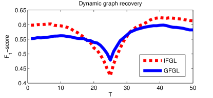
(a)

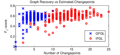
(b)

Figure 1: Comparison of generalization performance between GFGL and IFGL, for a dataset of size $P=10$, $T=50$. (a) $F_{1}$-score as a function of time $t$, plotted lines are the averages over $N_{\mathrm{test}}=200$ time-series. Error-bars are omitted for presentation, with an estimated standard deviation in the $F_{1}$-scores of $\sigma_{\mathrm{IFGL}}\approx 0.15$ and $\sigma_{\mathrm{GFGL}}\approx 0.14$. (b) Demonstration of GFGL and IFGL graph recovery as a function of the number of estimated changepoints $|\hat{\mathcal{T}}|$.

For each training time-series an optimal set of parameters are chosen which maximise the $F_{1}$-score, namely $\{(\lambda_{1}^{*},\lambda_{2}^{*})_{i}=\arg\max\>F_{1}(\lambda_{1},\lambda_{2})_{i}\}_{i=1}^{N_{\mathrm{train}}}$. The final, learnt optimal parameters $(\lambda_{1}^{*},\lambda_{2}^{*})$, are computed as the median value in this training set. A hold-out test set of independently simulated time-series is then used to measure the generalization performance. Figure 1a provides a typical comparison of the graph-recovery ($F_{1}$-score) performance between the IFGL and GFGL methods throughout the time-series duration. In this example it can be seen that IFGL tends to perform best at points far from the changepoint, whereas GFGL shows a benefit when estimating a graph close to the changepoint.

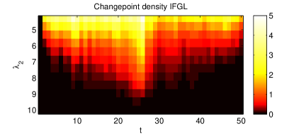
(a)

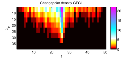
(b)

Figure 2: Changepoint density plots for IFGL and GFGL in the synthetic setting ($P=10,\;T=50,\;M=10\;\lambda_{1}=0.2$), there is a simulated changepoint at $\mathcal{T}=25$. Color represents the average number of edges (over $N=100$ simulations) which experience a change at a given time point.

We note the primary difference between IFGL and GFGL is the number of edges effected at each changepoint. This is demonstrated more clearly in Fig. 2. Here $\lambda_{1}$ is fixed and the number of edges which change at each time-point is plotted over a range of smoothing parameters $\lambda_{2}$. Clearly, GFGL results in a greater number of edges being effected at each changepoint. Due to the grouped estimation of GFGL a good level of graph recovery $F_{1}$-score performance is achievable with only a few changepoints (see Figure 1b). In contrast, if one sets $\lambda_{2}$ to be large in the IFGL setting, only a few changepoints are selected; however these represent changes in only very few edges (Fig. 2a). In this setting IFGL may perform well with regards to changepoint performance but this comes at the expense of poorer graph recovery as is evident from the $F_{1}$-scores. Where such grouped changepoint structure is present across many edges, GFGL enables one to recover changepoints without sacrificing as much graphical recovery performance.

4.4 Performance scaling

In this section, the recovery performance of the estimators is considered over a range of different problem sizes. In order to assess changepoint estimation performance and how this varies with scale, it is insightful to construct an error measure that monitors the average distance (in time) between estimated and true changepoints. The changepoints for a given edge $(i,j)$ can be described by considering differences in the precision matrix, i.e. $\hat{\mathcal{T}}_{ij}=\big{\{}t\colon\big{|}\hat{\Theta}_{ij}^{t}-\hat{\Theta}_{ij}^{t-1}\big{|}\neq 0,\>t=2,\ldots,T\big{\}}=:\{\hat{\tau}_{ij}^{k}\}_{k=1}^{\hat{K}_{ij}}$, with $\hat{K}_{ij}=\big{|}\hat{\mathcal{T}}_{ij}\big{|}$. These are compared with the ground truth changepoints for the $i,j$th edge ($\tau_{ij}$) from the changepoint set $\mathcal{T}_{ij}$ via the mean absolute error measure, namely $\text{MAE}:=\frac{1}{\hat{K}}\sum_{i,j}\sum_{k=1}^{\hat{K}_{ij}}\left|\hat{\tau}_{ij}^{k}-\tau_{ij}\right|$, where $\hat{K}=\sum_{ij}\hat{K}_{ij}$ . In these experiments a single changepoint is shared across multiple edges at $\mathcal{T}={T/2}$. To allow fair comparison between experiments at different time-series lengths ($T$), the same precision matrices are used either side of the changepoint. For example, under scaling $T\rightarrow 2T$, the number of data-points either side of the changepoint is simply doubled. When considering scaling with respect to dimension precision matrices are simulated as discussed in Sec. (4.1); however the number of active edges scaled as $M=P$. Experiments were run with data-sets of size $N_{\mathrm{train}}=20$ and $N_{\mathrm{test}}=200$ and optimal lambdas were selected through $F$-score maximization.

(a)

(b)

(c)

Figure 3: Estimator performance and scaling: (a) $F_{1}$-score vs time-series length; (b) relative changepoint error ($MAE/T$) as a function of increasing time-series length $T$; (c) $F_{1}$-score vs dimension $P$. Error bars represent 67% confidence intervals as estimated from the empirical c.d.f. of $N=200$ test examples.

The results presented in Fig. 3 demonstrate that recovery performance improves as more data is made available (increasing $T$) and degrades as the problem task becomes more complex (increasing $P$). On average IFGL performs slightly better at estimating the correct edges. However GFGL performs better in the changepoint detection task where the relative changepoint error reduces at an improved rate as $T$ is increased. Such a result coincides with the performance demonstrated in Fig. 1 where GFGL outperforms in the vicinity of a changepoint. If grouped changepoints are present the experiments suggest GFGL performs better in the changepoint estimation task without sacrificing graph recovery performance.

The results here display how recovery performance scales with problem dimensionality. However such performance will also depend on the structure of the ground-truth graph and precision matrices. As an example, in the stationary setting Ravikumar et al. (2011) suggests that, for consistent recovery of graphs (with $N$ data-points), one should bound the partial correlations, $[-1,-\alpha]\cup[\alpha,1]$, such that $\alpha=\Omega(\sqrt{\log P/N})$. To enable better interpretation of experimental results we fixed $\alpha=1/2$ in these examples. However, it is anticipated that changepoint and graph estimation may become more difficult as the true non-zero partial correlations $\Theta_{i,j}$ tend towards zero.

4.5 Computational Complexity

In order to investigate computational scalability, a series of experiments were performed on problems of various size (the experimental setup is the same as in Sec. 4.4), the results are summarized in Figure 4.

(a)

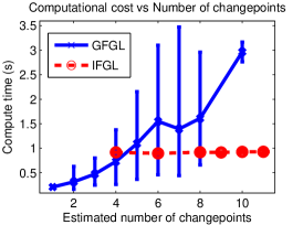
(b)

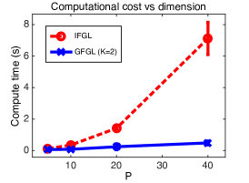
(c)

Figure 4: Empirical computational performance of ADMM for GFGL: (a) Compute-time vs time-series length $T$ for a fixed number of changepoints; (b) Compute-time vs number of estimated changepoints $\hat{|\mathcal{T}|}$; (c) Compute-time as a function of dimension $P$.

In contrast with the quadratic time complexity for dynamic programming methods (Angelosante and Giannakis, 2011), it can be observed that the ADMM routine, as a whole, maintains roughly linear complexity with increasing $T$. When considering increases in the estimated number of changepoints $\hat{K}$, complexity appears to follow the quadratic rate of GFLseg (used in Algorithm 2), which scales as $\approx\mathcal{O}(TP^{2}\hat{K}^{2})$, see Bleakley and Vert (2011).

5 Example: Time Evolution of Genetic Dependency Networks

In this section we give an example of how methods such as GFGL can be used in an applied context. In recent years it has become increasingly common to construct experiments which sample gene-expression activity as a time-series. As an example of such data, we consider the genetic activity of a fruit-fly (D. melanogaster) from its embryonic birth to final adult state. The dataset we analyze is a subset of the data collected by Arbeitman et al. (2002), which measures gene expression patterns for 4096 genes, approximately one third of all D. melanogaster genes, over $T=67$ time-points.

To aid interpretation of the results and for computational feasibility, we consider a smaller subset of genes ($P=150$), which are understood to be linked to certain biological processes, in this case, immune system response. The link between this subset of genes and biological function is motivated by considering conserved co-domains of a gene. Where such co-domains are shared between genes, one can often infer a similar biological function of the genes, this similarity can be extended to other organisms if the genes are homologous (Forslund et al., 2011). In this case, our selection of genes is based on the Flybase (Attrill et al., 2016) Gene-ontology database. Understanding the dependency between genes involved in a certain process is interesting to biologists who want to examine and understand why or how regulation of gene activity evolves over time— for example after an intervention or treatment. Previous work on this data-set by Lèbre et al. (2010) considered estimating changepoints in a causal VAR-type model. In contrast to this work, we are concerned with estimating the contemporaneous relationships between genes. Specifically, we model the innovations $\boldsymbol{\epsilon}_{t}$, where $Y_{t}=Y_{t-1}+\boldsymbol{\epsilon}_{t}\;\mathrm{where}\;\boldsymbol{\epsilon}_{t}\sim\mathcal{N}(\boldsymbol{0},\boldsymbol{\Theta}^{t})\;.$

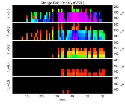
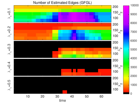
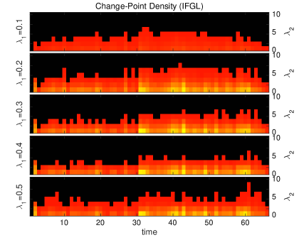
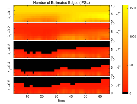
Figure 5: Changepoint density (the color indicates the number of edges which change) and the number of edges recovered as function of both time and tuning parameters.

Unlike in the synthetic experiments, the time-course data analyzed here was not replicated, i.e. we only have one data-point at each time point in the fly’s development. It is worth noting that more recent experiments involving time-course microarray data may produce replicated experiments. These are thought to be particularly valuable, as it allows one to gauge the uncertainty due to variation in genetic populations and environmental factors. With such replicated experiments, there may also be a meaningful way to perform cross-validation to estimate the hyper-parameters. However, in the absence of replicates, we adopt an exploratory approach and consider the inferred structure over a wide range of regularization parameters. We scan over the range $\lambda_{1}=0.1$ to $0.5$ for both methods, with $\lambda_{2}=80$ to $200$ for GFGL, and $\lambda_{2}=1$ to $10$ in the IFGL case.

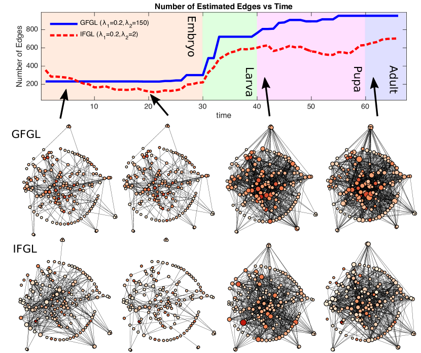
Figure 6: Top: Estimated Edges as a function of time with overlay of physiological life-cycle stages. Bottom: Estimated graph structure for GFGL and IFGL at 4 different time-points ($t=5,t=20,t=40,t=62$), size of node indicates degree, the positions of nodes (representing individual genes) are comparable across graphs.

Figure 5 demonstrates how both the sparsity, number and position of changepoints in the solution behave as a function of $\lambda_{1},\lambda_{2}$. One can clearly see that both smoothing (the number of changepoints) and sparsity (the number of edges) are linked to $(\lambda_{1},\lambda_{2})$ jointly. For a given selection of $\lambda_{1},\lambda_{2}$ we obtain an estimate of the dynamic graph, some snapshots of such graphs are illustrated in Fig. 6. In this example, the graphs are drawn such that gene-positions (vertices) are comparable both across time and between methods. This application to genetic data clearly illustrates the qualitative differences between the estimators in terms of extracted structure. In both methods we observe that more edges are detected in the later-half of the life-cycle, with a large change in structure inferred during the Larval stage of development. Unlike IFGL, which experiences changepoints at all time-points, GFGL clearly has more pronounced jumps; i.e. more edges change at each changepoint (see Fig. 5). Additionally, if one considers the varying size of node (proportional to degree) it appears that the degree of the GFGL estimates are more stable. Such a feature suggests that the particular GFGL estimate (in Fig. 6) has fewer degrees of freedom than the IFGL estimate. Such a property may be appealing in the high-dimensional setting, where GFGL appears to permit similar graphical structure, but with enhanced temporal stability in the graph.

6 Discussion

Two classes of estimators have been investigated for piecewise constant GGM. In particular, we have proposed the GFGL estimator for grouped estimation of changepoints in a dynamic GGM. Empirical results suggest that GFGL has similar model recovery abilities to the IFGL class of estimators. However, when simultaneous grouped changepoints are expected to occur, the group-fused estimator does not appear to sacrifice as much graph-recovery performance in order to accurately estimate changepoints. Further to this, when estimating grouped changepoints, the group-fused estimator appears to converge to the true changepoints at a faster rate. We find that the grouped approach offers a more meaningful and interpretable segmentation of the graphical dynamics. This is especially apparent when such grouped changes represent systemic phase or regime changes in activity. When one has a priori knowledge of grouping, it is anticipated that GFGL will offer a useful and scalable investigative tool to support data exploration and subsequent inference.

Our empirical results on the relative changepoint error and F-score vs $T$ suggest convergence of the estimator. However, we leave further theoretical examination of such consitency properties as future work. A possible way forward here is to exploit the theory developed for the individual subproblems, namely changepoint detection with the lasso (Harchaoui and Lévy-Leduc, 2010) and sparse group lasso (Zhang et al., 2014; Simon et al., 2013). Such work may build on results in the dynamic graph learning setting by Kolar and Xing (2011, 2012) and Roy et al. (2015).

7 Supplemental Materials

An Appendix containing technical details and further information can be found in the on-line supplemental material for this paper. In addition to the Appendix, one can also find a compressed folder with example code to implement the GFGL and IFGL estimators as discussed in the paper.

References

- Ahmed and Xing (2009) Ahmed, A. and Xing, E. P. “Recovering time-varying networks of dependencies in social and biological studies.” Proceedings of the National Academy of Sciences of the United States of America, 106(29):11878–83 (2009).
- Alaíz et al. (2013) Alaíz, C. M., Barbero, A., and Dorronsoro, J. R. “Group Fused Lasso.” Artificial Neural Networks and Machine Learning - ICANN 2013, 66–73 (2013).
- Angelosante and Giannakis (2011) Angelosante, D. and Giannakis, G. B. “Sparse graphical modeling of piecewise-stationary time series.” IEEE International Conference on Acoustics, Speech and Signal Processing (ICASSP), 1960–1963 (2011).
- Arbeitman et al. (2002) Arbeitman, M. N., Furlong, E. E. M., Imam, F., Johnson, E., Null, B. H., Baker, B. S., Krasnow, M. A., Scott, M. P., Davis, R. W., and White, K. P. “Gene expression during the life cycle of Drosophila melanogaster.” Science, 297(5590):2270–5 (2002).
- Attrill et al. (2016) Attrill, H., Falls, K., Goodman, J. L., Millburn, G. H., Antonazzo, G., Rey, A. J., and Marygold, S. J. “FlyBase: establishing a Gene Group resource for Drosophila melanogaster.” Nucleic Acids Research, 44(D1) (2016).
- Banerjee et al. (2008) Banerjee, O., El Ghaoui, L., and D’Aspremont, A. “Model selection through sparse maximum likelihood estimation for multivariate gaussian or binary data.” The Journal of Machine Learning Research, 1–35 (2008).
- Banerjee et al. (2007) Banerjee, O., Ghaoui, L. E., and D’Aspremont, A. “Model Selection Through Sparse Maximum Likelihood Estimation for Multivariate Gaussian or Binary Data.” Journal of Machine Learning Research (2007).
- Bleakley and Vert (2011) Bleakley, K. and Vert, J. P. “The group fused Lasso for multiple change-point detection.” arXiv preprint arXiv:1106.4199, 1–24 (2011).
- Boyd et al. (2011) Boyd, S., Parikh, N., and Chu, E. “Distributed optimization and statistical learning via the alternating direction method of multipliers.” Foundations and Trends in Machine Learning, 3(1):1–122 (2011).
- Chun et al. (2014) Chun, H., Zhang, X., and Zhao, H. “Gene regulation network inference with joint sparse Gaussian graphical models.” Journal of Computational and Graphical Statistics, (April 2015):00–00 (2014).
- Combettes and Pesquet (2011) Combettes, P. L. and Pesquet, J. C. “Proximal splitting methods in signal processing.” Fixed-point algorithms for inverse problems for Inverse Problems in Science and Engineering, 1–25 (2011).
- Danaher et al. (2013) Danaher, P., Wang, P., and Witten, D. M. “The joint graphical lasso for inverse covariance estimation across multiple classes.” Journal of the Royal Statistical Society: Series B (Statistical Methodology) (2013).
- Drton and Perlman (2004) Drton, M. and Perlman, M. D. “Model selection for Gaussian concentration graphs.” Biometrika, 91(3):591–602 (2004).
- Eckstein and Bertsekas (1992) Eckstein, J. and Bertsekas, D. P. “On the Douglas-Rachford splitting method and the proximal point algorithm for maximal monotone operators.” Mathematical Programming (1992).
- Forslund et al. (2011) Forslund, K., Pekkari, I., and Sonnhammer, E. L. “Domain architecture conservation in orthologs.” BMC Bioinformatics, 12(1):326 (2011).
- Friedman et al. (2007) Friedman, J., Hastie, T., Hoefling, H., and Tibshirani, R. “Pathwise coordinate optimization.” Annals of Applied Statistics (2007).
- Friedman et al. (2008) Friedman, J., Hastie, T., and Tibshirani, R. “Sparse inverse covariance estimation with the graphical lasso.” Biostatistics (Oxford, England), 9(3):432–41 (2008).
- Gibberd and Nelson (2014) Gibberd, A. J. and Nelson, J. D. B. “High dimensional changepoint detection with a dynamic graphical lasso.” IEEE International Conference on Acoustics, Speech and Signal Processing (ICASSP) (2014).
- Glowinski and Le Tallec (1989) Glowinski, R. and Le Tallec, P. Augmented Lagrangian and Operator-Splitting Methods in Nonlinear Mechanics. SIAM (1989).
- Harchaoui and Lévy-Leduc (2010) Harchaoui, Z. and Lévy-Leduc, C. “Multiple Change-Point Estimation With a Total Variation Penalty.” Journal of the American Statistical Association, 105(492):1480–1493 (2010).
- Kolar and Xing (2011) Kolar, M. and Xing, E. P. “On Time Varying Undirected Graphs.” Proceedings of the International Conference on Artificial Intelligence and Statistics (AISTATS), 15:407–415 (2011).
- Kolar and Xing (2012) —. “Estimating networks with jumps.” Electronic Journal of Statistics, 6:2069–2106 (2012).
- Lafferty et al. (2012) Lafferty, J., Liu, H., and Wasserman, L. “Sparse Nonparametric Graphical Models.” Statistical Science, 27(4):519–537 (2012).
- Lauritzen (1996) Lauritzen, S. L. Graphical Models. Oxford (1996).
- Lèbre et al. (2010) Lèbre, S., Becq, J., Devaux, F., Stumpf, M. P. H., and Lelandais, G. “Statistical inference of the time-varying structure of gene-regulation networks.” BMC systems biology, 4:130 (2010).
- Lee and Hastie (2015) Lee, J. D. and Hastie, T. J. “Learning the Structure of Mixed Graphical Models.” Journal of Computational and Graphical Statistics, 24(1):230–253 (2015).
- Liu et al. (2010) Liu, J., Yuan, L., and Ye, J. “An efficient algorithm for a class of fused lasso problems.” Proceedings of the 16th ACM SIGKDD International Conference on Knowledge Discovery and Data Mining, 323 (2010).
- Monti et al. (2014) Monti, R. P., Hellyer, P., Sharp, D., Leech, R., Anagnostopoulos, C., and Montana, G. “Estimating time-varying brain connectivity networks from functional MRI time series.” NeuroImage (2014).
- Parikh and Boyd (2013) Parikh, N. and Boyd, S. “Proximal algorithms.” Foundations and Trends in optimization, 1(3):123–231 (2013).
- Ravikumar et al. (2011) Ravikumar, P., Wainwright, M. J., Raskutti, G., and Yu, B. “High-dimensional covariance estimation by minimizing l1-penalized log-determinant divergence.” Electronic Journal of Statistics, 5(January 2010):935–980 (2011).
- Roy et al. (2015) Roy, S., Atchad, Y., and Michailidis, G. “Change-Point Estimation in High-Dimensional Markov Random Field Models.” arXiv preprint arXiv:1405.6176v2 (2015).
- Simon et al. (2013) Simon, N., Friedman, J., Hastie, T., and Tibshirani, R. “A Sparse-Group Lasso.” Journal of Computational and Graphical Statistics, 22(2):231–245 (2013).
- Tibshirani (1996) Tibshirani, R. “Regression shrinkage and selection via the lasso.” Journal of the Royal Statistical Society: Series B (Statistical Methodology) (1996).
- Tseng and Yun (2009) Tseng, P. and Yun, S. “A coordinate gradient descent method for nonsmooth separable minimization.” Mathematical Programming (2009).
- Wang (2012) Wang, H. “Bayesian Graphical Lasso Models and Efficient Posterior Computation.” Bayesian Analysis, 7(4):867–886 (2012).
- Yang et al. (2015) Yang, S., Lu, Z., Shen, X., Wonka, P., and Ye, J. “Fused Multiple Graphical Lasso.” SIAM Journal on Optimization, 25 (2015).
- Yuan and Lin (2006) Yuan, M. and Lin, Y. “Model selection and estimation in regression with grouped variables.” Journal of the Royal Statistical Society (2006).
- Yuan (2011) Yuan, X. “Alternating Direction Method for Covariance Selection Models.” Journal of Scientific Computing, 51(2):261–273 (2011).
- Zhang et al. (2014) Zhang, B., Geng, J., and Lai, L. “Multiple Change-Points Estimation in Linear Regression Models via Sparse Group Lasso.” IEEE Trans. Signal Processing (2014).
- Zhou et al. (2010) Zhou, S., Lafferty, J., and Wasserman, L. “Time varying undirected graphs.” Machine Learning, 80(2-3):295–319 (2010).