Ab initio atom–atom potentials using CamCASP: Theory and application to multipole models for the pyridine dimer.

Abstract

Creating accurate, analytic atom–atom potentials for small organic molecules from first principles can be a time-consuming and computationally intensive task, particularly if we also require them to include explicit polarization terms, which are essential in many systems. In this first part of a two-part investigation, we describe how the CamCASP suite of programs can be used to generate such potentials using some of the most accurate electronic structure methods currently applicable. In particular, we derive the long-range terms from monomer properties, and determine the short-range anisotropy parameters by a novel and robust method based on the iterated stockholder atom approach. We use the techniques described here to develop distributed multipole models for the electrostatic, polarization and dispersion interactions in the pyridine dimer. In the second part of this work we will apply these methods to develop a series of many-body potentials for the pyridine system.

I Introduction

Electronic structure methods for the interaction energy have come a long way since the mid-nineties, when the water dimer represented the largest system for which accurate, ab initio intermolecular interaction energies could be calculated. We can now calculate interaction energies for small organic molecules like pyridine and benzene in hours on a single processor Podeszwa et al. (2006); Hesselmann et al. (2005, 2006), and medium sized molecules like cyclotrimethylene trinitramine (RDX) Podeszwa et al. (2007), base pairs Hesselmann et al. (2006), and tetramers of amino acids Fiethen et al. (2008). Part of the reason for this is the increase in our computational resources, but more important are the new developments in electronic structure methods. For the field of intermolecular interactions, the development of symmetry-adapted perturbation theory based on density-functional theory, or SAPT(DFT), has done much to improve both the accuracy and the range of applicability of theoretical methods. Misquitta and Szalewicz (2002); Misquitta et al. (2003); Misquitta and Szalewicz (2005); Misquitta et al. (2005); Podeszwa et al. (2006); Hesselmann and Jansen (2002, 2002, 2003); Hesselmann et al. (2005)

However, such calculations cannot be used on the fly in most molecular simulations, as the computational cost is too high, and we need to represent the interaction energy by an analytic potential. Such potentials are commonly expressed in terms of the many-body expansion, where the interaction energy of a cluster of interacting molecules is partitioned into two-body contributions plus corrections arising from triplets, quartets and larger clusters of molecules. That is,

$$V_{ABC\dots}=\sum_{X\mathchar 12604\relax Y}V_{XY}+\sum_{X\mathchar 12604\relax Y\mathchar 12604\relax Z}\Delta V_{XYZ}+\cdots,$$ (1)

where $V_{XY}$ is the interaction energy between molecules $X$ and $Y$ in the absence of all other molecules, but in the geometry found in the complete system, while $\Delta V_{XYZ}$ is the three-body correction, defined as

$$\Delta V_{XYZ}=V_{XYZ}-V_{XY}-V_{XZ}-V_{YZ}$$

and $V_{XYZ}$ is the energy of the $XYZ$ cluster in the absence of all other molecules, but in the geometry found in the complete system. Four-body, five-body and other many-body corrections are defined in a similar manner.

The success of this expansion depends on its rapid convergence. In any molecular system with distinct interacting units, the two-body terms will dominate, but the many-body terms can contribute as much as 30% of the interaction energy for clusters of polar molecules Hodges et al. (1997); Mas et al. (2003, 2003), and can be essential for getting the structure and properties correct. For example, three and four-body effects have been shown to be responsible for the tetrahedral structure of liquid water Bukowski et al. (2006). The many-body polarization energy has also been shown to be an important discriminator in the relative lattice energies of molecular crystals when the structures differ considerably in their hydrogen-bonding motifs Welch et al. (2008).

A three-body implementation of SAPT(DFT) does exist Podeszwa and Szalewicz (2007), but the computational cost makes on-the-fly methods even more impractical, and although three-body non-additive interactions make up the bulk of the many-body non-additivity in systems like water, non-additive effects beyond this level cannot be neglected Bukowski et al. (2006). If the constituent bodies in a cluster are small enough, it would be possible to use an electronic structure method like SAPT(DFT) or CCSD(T) (coupled-cluster singles and doubles with non-iterated triples) for the two and three-body terms in the many-body expansion, and an appropriate approximation for the other terms. But more generally this approach would make formidable computational demands, and it is necessary to use analytic intermolecular potentials in many applications.

Analytic intermolecular potentials have been in use for many decades. (See ref. 20 for a review.) In the past, most have been ‘pair potentials’, including only two-body terms. In any molecular system with distinct interacting units, the two-body terms will dominate, but the many-body terms can be essential for getting the structure and properties correct. The effects of many-body terms have often been included in an approximate ‘average’ manner through adjustment of the empirical parameters. This is done in empirical potentials for water, which typically feature an enhanced dipole moment to mimic the increased average dipole of the water molecule in the condensed phase. While such pair potentials are still widely used, it is increasingly recognised that it is necessary to take account of the many-body effects explicitly, particularly to account for the effects of electrostatic polarization Jiang et al. (2007); Welch et al. (2008); Illingworth and Domene (2009), but also to account for many-body dispersion effects Bukowski et al. (1999); Bukowski and Szalewicz (2001); Kim et al. (2006), and, as we shall see, to account for intermolecular charge delocalisation, or charge transfer (CT).

Potentials with this level of complexity, accuracy and detail cannot be obtained empirically. Instead we must turn to theoretical methods. Ab initio-derived potentials are by no means new, and indeed there are a number of accurate potentials in the published literature (see for example refs. 26; 27; 28; 29). These potentials have typically been obtained for small dimers, but recently examples involving medium sized systems have become available Podeszwa et al. (2006, 2007); Misquitta et al. (2008); Totton et al. (2010). There are a few common ideas used in the creation of these and other ab initio potentials. The first is that they are all based on a distributed model; that is, the interaction energy between molecules is represented as the sum of contributions between pairs of atoms. Secondly, most are not polarizable, so many-body polarization terms are missing (though polarization may be included at the two-body level). Thirdly, in all cases, long-range parameters have been derived from the unperturbed molecules, which can dramatically simplify the number of free parameters in the fit. Finally, the short-range parameters are usually then fitted to a set of ab initio interaction energies calculated using a suitable electronic structure method.

The above procedure works reasonably well, but it has a number of deficiencies. First and foremost is the usual lack of many-body polarization effects. Second, there is much uncertainty associated with fitting the short-range exponential terms in a system of medium sized molecules. These uncertainties are largely related to sampling: we are usually not sure that we have enough data to define the terms in the potential. This is particularly troublesome for the larger systems, which not only have a larger number of free parameters to fit, but which also incur considerable computational expense to calculate the ab initio interaction energies needed for the fit. Additionally, the short-range terms are usually exponential in form, and it is very difficult to fit a sum of exponentials while also requiring that the fit parameters remain physically sensible and transferable. Some of these difficulties can be partially alleviated by iterating the process and adding additional data at important configurations Podeszwa et al. (2006), but on the whole this approach is unsatisfactory and tedious, and an alternative is needed.

The alternative we describe in this paper is to compute directly most of the potential parameters, including those associated with the short-range part of the potential, and keep the fitting to a minimum. In many ways this is not a new strategy; indeed, a similar technique has been implemented by Schmidt and co-workers Yu et al. (2011); McDaniel and Schmidt (2013); Schmidt et al. (2015), who have used many of the techniques we will describe in this paper to develop a family of transferable potentials with a strong physical basis. However, so far these have been isotropic potentials of moderate accuracy, with a strong focus on ease of creation and transferability. As we will demonstrate here, we bring a new level of fidelity, accuracy and reliability to the procedure, using the many tools we have developed in recent years and have implemented in the CamCASP Misquitta and Stone (2016) program. We begin this paper with a description of the overall strategy, then describe some of the algorithms we have implemented in the CamCASP suite of programs to implement the strategy. In particular, partitioning the electron density using the iterated stockholder atom procedure is very effective in overcoming the difficulties in fitting the short-range potential. In the second paper we apply these methods to the pyridine dimer and discuss the resulting potentials.

II The problem and definitions

The goal is to find an analytic potential $V_{\text{int}}$ that accurately models the two-body SAPT(DFT) interaction energy

$$E_{\rm int}^{(1-\infty)} =E^{(1)}_{\rm elst}+E^{(1)}_{\rm exch}+E^{(2)}_{\rm IND}+E^{(2)}_{\rm DISP}+\delta^{\rm HF}_{\rm int}.$$ (2)

(We will use $E$ throughout to denote the computed energy terms and $V$ to denote their analytic representations.) Here $E^{(1)}_{\rm elst}$ and $E^{(1)}_{\rm exch}$ are the first-order electrostatic and exchange-repulsion energies, $E^{(2)}_{\rm IND}=E^{(2)}_{\rm ind,pol}+E^{(2)}_{\rm ind,exch}$ is the total second-order induction energy, $E^{(2)}_{\rm DISP}=E^{(2)}_{\rm disp,pol}+E^{(2)}_{\rm disp,exch}$ is the total dispersion energy Jansen (2015), and $\delta^{\rm HF}_{\rm int}$ is the estimate of effects of third and higher order, primarily induction Jeziorska et al. (1987); Moszynski et al. (1996). The broad strategy we have adopted to determine $V_{\text{int}}$ has been described in some detail in a review article Stone and Misquitta (2007). While many of the details have changed, the essence of the method remains as described there, so only a high-level description will be provided here.

First of all, we represent the potential $V_{\text{int}}$ as

$$V_{\text{int}} =\sum_{a\in A}\sum_{b\in B}V_{\text{int}}[ab](r_{ab},\Omega_{ab}),$$ (3)

where, $a$ and $b$ label sites (usually taken to be atomic sites) in the interacting molecules $A$ and $B$, $r_{ab}$ is the inter-site separation, $\Omega_{ab}$ is a suitable set of angular coordinates that describes the relative orientation of the local axis systems on these sites (see ch. 12 in ref. 20), and $V_{\text{int}}[ab]$ is the site–site potential defined as

$$V_{\text{int}}[ab]=V_{\rm sr}[ab]+V_{\text{elst}}[ab]+V_{\text{disp}}[ab]+V_{\text{pol}}[ab].$$ (4)

The terms in $V_{\text{int}}[ab]$ model the corresponding terms in $E_{\rm int}^{(1-\infty)}$. $V_{\rm sr}[ab]$ is the short-range term, which mainly describes the exchange–repulsion energy, but also includes some other short-range effects, discussed in §VI:

$$V_{\rm sr}[ab]=G\exp{[-\alpha_{ab}(\Omega_{ab})(r_{ab}-\rho_{ab}(\Omega_{ab}))]},$$ (5)

where $\rho_{ab}(\Omega_{ab})$ is the shape function for this pair of sites, which depends on their relative orientation $\Omega_{ab}$, and $\alpha_{ab}$ is the hardness parameter which may also be a function of orientation. $G$ is a constant energy which we will take to be $10^{-3}$ hartree. $V_{\text{elst}}[ab]$ is the expanded electrostatic energy:

$$V_{\text{elst}}[ab]=V_{\text{elst}}[ab]\bigl{(}r_{ab},\Omega_{ab},Q^{a}_{t},Q^{b}_{u},\beta_{\rm elst}^{ab}\bigr{)};$$ (6)

$Q^{a}_{t}$ is the multipole moment of rank $t$ for site $a$, where, using the compact notation of ref. 20, $t=00,10,11c,11s,\cdots$, and $\beta_{\rm elst}^{ab}$ is a damping parameter. The dispersion energy $V_{\text{disp}}[ab]$ depends on the anisotropic dispersion coefficients $C_{n}^{ab}(\Omega_{ab})$ for the pair of sites, and on a damping function $f_{n}$ that we will take to be the Tang–Toennies Tang and Toennies (1992) incomplete gamma functions of order $n+1$:

$$V_{\text{disp}}[ab]=-\sum_{n=6}^{12}f_{n}\Bigl{(}\beta_{\rm disp}^{ab}r_{ab}\Bigr{)}C_{n}^{ab}(\Omega_{ab})r_{ab}^{-n}$$ (7)

The final term $V_{\text{pol}}[ab]$ is the polarization energy, which is the long-range part of the induction energy Misquitta (2013). $V_{\text{pol}}[ab]$ depends on the multipole moments and the polarizabilities $\alpha^{a}_{tu}$, which are indexed by pairs of multipole components $tu$ (for details see refs.43; 20):

$$V_{\text{pol}}[ab]=V_{\text{pol}}[ab]\bigl{(}Q^{a}_{t},Q^{b}_{u},\alpha^{a}_{tu},\alpha^{b}_{tu},\beta_{\rm pol}^{ab}\bigr{)}.$$ (8)

There are a few points to note about the particular form of the potential $V_{\text{pol}}[ab]$. Although formally written in the form of a two-body potential, many-body polarization effects are included through the classical polarization expansion Stone (2013). Also, we will normally define the multipole moments and polarizabilities to include intramolecular many-body effects implicitly, that is, we use the multipoles and polarizabilities of atoms-in-a-molecule, localized appropriately. To this form of the potential we could add a three-body dispersion model, but this is not addressed in this paper.

III Strategy

There are many parameters in such a potential and our goal is to compute as many of these parameters as possible, and keep the fitting of the remainder to a minimum. Additionally, we will adopt a hierarchical approach to the fitting process that helps to guarantee confidence in the parameter values. There are three main parts to the process, and these involve the following:

• Long-range terms: The electrostatic, polarization and dispersion interaction energy components possess expansions in powers of $1/R$, where $R$ is the centre-of-mass separation (for small systems) or, more generally, the inter-site distance in a distributed expansion. Multipole moments are functions of the unperturbed molecular densities and may be derived using a variety of methods, the most common being the distributed multipole analysis (DMA) technique Stone and Alderton (1985); Stone (2005). But, using a basis-space algorithm of the iterated stockholder atom (ISA) procedureLillestolen and Wheatley (2009) termed the BS-ISA algorithm Misquitta et al. (2014), we have demonstrated that the ISA/BS-ISA-based distribution yields a more rapidly convergent multipole expansion with properties that make it ideal for modelling. The distributed polarizabilities and dispersion coefficients are obtained using the Williams–Stone–Misquitta (WSM) technique Misquitta and Stone (2006, 2008); Misquitta et al. (2008); Misquitta and Stone (2008). With this approach we may consider the long range parameters in the potential $V_{\text{int}}$ as fixed, though, we may optionally tune them if appropriate.

• Damping: All three multipole expansions need to be damped at short range, when overlap effects become appreciable and the $1/R$ terms start to exhibit mathematical divergences. Damping will not be applied to the electrostatic expansion as it is not usually needed, but it can be applied if necessary Stone (2011). It is crucial to damp the polarization and dispersion expansions as the mathematical divergence of these expansions is usually manifest at accessible separations, and must be controlled if sensible expansions are needed. For the dispersion expansion we use a single damping coefficient based on the vertical ionization potentials $I_{A}$ and $I_{B}$ (measured in atomic units) of the interacting molecules Misquitta and Stone (2008):

  $$\beta_{\rm disp}^{ab}\equiv\beta_{\rm disp}^{AB}=\sqrt{2I_{A}}+\sqrt{2I_{B}}.$$ (9)

  This single-parameter damping is almost certainly not ideal, and we should rather use damping parameters that depend on the atomic types, and optionally, on their relative orientation. We will propose such a more elaborate, but still non-empirical model in a forthcoming paper Van Vleet et al. (2015).

  The damping of the polarization expansion is less straightforward and will be discussed in detail below.

• Short-range energies: If the damped multipole (DM) expanded energies are removed from the interaction energy $E_{\rm int}^{(1-\infty)}$, we obtain the remainder which is the short-range energy:

  $$E_{\rm sr}^{(1-\infty)} =E^{(1)}_{\rm exch}+(E^{(1)}_{\rm elst}-V^{(1)}_{\rm elst}[{\rm DM}])$$

  $$\quad+(E^{(2)}_{\rm IND}+\delta^{\rm HF}_{\rm int}-V^{(2-\infty)}_{\rm pol}[{\rm DM}])$$

  $$\quad+(E^{(2)}_{\rm DISP}-V^{(2)}_{\rm disp}[{\rm DM}])$$

  $$=E_{\rm sr}^{(1)}+E_{\rm sr}^{(2-\infty)}.$$ (10)

  Here we have partitioned the short-range energy into a first-order contribution $E_{\rm sr}^{(1)}$ which will be dominant, and the second- to infinite-order contribution $E_{\rm sr}^{(2-\infty)}$ which will be primarily the infinite-order charge-transfer energy. In the above expression, $V^{(1)}_{\rm elst}[{\rm DM}]$ and $V^{(2)}_{\rm disp}[{\rm DM}]$ are the multipole expanded forms of the electrostatic and dispersion energies, and $V^{(2-\infty)}_{\rm pol}[{\rm DM}]$ is the infinite-order (iterated) multipole-expanded polarization energy. In principle, the various contributions to $E_{\rm sr}^{(1-\infty)}$ are not expected to depend on dimer geometry in the same way and they should be modelled separately. However, we have previously showed that the dominant contributions to $E_{\rm sr}^{(1)}$ —the first-order exchange and penetration energies—are proportional to each other,Misquitta et al. (2014) and here we will show that the charge-transfer contribution is also nearly proportional, so we shall model all parts of $E_{\rm sr}^{(1-\infty)}$ together as a single sum of exponential terms:

  $$V_{\rm sr} =\sum_{a\in A}\sum_{b\in B}V_{\rm sr}[ab]$$ (11)

  where each $V_{\rm sr}[ab]$ has the form of eq. (5).

• Sampling dimer configuration space: In order to ensure a balanced fit, it is important to ensure that we sample the six dimensional dimer configuration space adequately. For such a high dimensional space the sampling needs to be (quasi) random, and in earlier work Misquitta et al. (2008); Stone and Misquitta (2007); Totton et al. (2010) we have described how this can be done using a quasi random Sobol sequence and Shoemake’s algorithm Shoemake (1992) (see the supplementary information for a brief description of this algorithm). This algorithm has been implemented in the CamCASP program and ensures that we cover orientation space randomly, but uniformly. Unless otherwise indicated, dimer configurations will be obtained using this algorithm.

• Fitting the short-range terms: first-order energies: A direct fit to the terms in $V_{\rm sr}$ usually leads to unphysical parameters and therefore should be avoided. Additionally, it is difficult to sample the high-dimensional configuration space densely enough to define the shape anisotropy of the interacting sites. This is particularly true for the larger molecular systems, for which the computational cost of calculating the second to infinite order SAPT(DFT) interaction energies can be appreciable, thus precluding the possibility of adequate sampling. One possibility in this case is to reduce the complexity of $V_{\rm sr}$ by, for example, keeping only isotropic terms in the expansions for the hardness parameter and the shape functions, but this may not be appropriate when high accuracies are needed.

  In previous work Misquitta et al. (2008) we addressed this problem using the density-overlap model Kita et al. (1976); Kim et al. (1981); Nobeli et al. (1998) to partition the first-order short-range energies, $E_{\rm sr}^{(1)}$, into contributions from pairs of atoms. This partitioning allows us to fit the terms for each pair of sites $ab$ and obtain a first guess at $V^{(1)}_{\rm sr}[ab]$, while avoiding fitting the sum of exponential terms directly. In §VI.2 we provide more detail on how this is done, and show how the parameters in eq. (11) can be determined with a high degree of confidence if we use a density partitioning method based on the ISA method. As we shall see, this procedure effectively eliminates the basis-set limitations seen in our earlier attempts. Moreover, this step uses the first-order energies only, and these energies are not only computationally inexpensive, but may be calculated using a monomer basis set, so a dense coverage of configuration space may be used to determine good initial guesses for the parameters in $V^{(1)}_{\rm sr}$. In this manner, atomic shape functions may be determined easily and reliably.

• Constrained relaxation: At various stages in the fitting process we will relax a fit with constraints applied. The idea here is to obtain a good guess for the parameters in the fit in a manner that ensures that they are well-defined. Subsequently, these parameters may be relaxed while pinning them to the predetermined values. Consider a fitting function $g(p_{0},p_{1},\cdots,p_{n})$, where $p_{i}$ are the free parameters in the fit. If our initial guess for these are $p^{0}_{i}$, then in a constrained relaxation we would optimize the function

  $$G(p_{0},p_{1},\cdots,p_{n}) =g(p_{0},p_{1},\cdots,p_{n})$$

  $$\qquad+\sum_{i=0}^{n}c_{i}(p_{i}-p^{0}_{i})^{2},$$ (12)

  where $c_{i}$ are suitable constraint strength parameters that should be associated with our confidence in the initial parameter guesses $p^{0}_{i}$. In a Bayesian sense, the ${p^{0}_{i}}$ are our prior values and the ${c_{i}}$ will be related to the prior distribution. As data is included, the parameters ${p_{i}}$ may deviate from their initial values. In this manner, a fit may be performed with very little data and we ensure that no parameter attains an unphysical value.

• Relaxing $V^{(1)}_{\rm sr}$ to $E_{\rm sr}^{(1)}$: Having obtained the first guess for $V^{(1)}_{\rm sr}$, we may now perform a constrained relaxation of the parameters in $V^{(1)}_{\rm sr}$ to fit $E_{\rm sr}^{(1)}$ better. Symmetry constraints to the shape-function parameters may also be imposed at this stage.

• Relaxing $V^{(1)}_{\rm sr}$ to include higher-order energies: The parameters in $V^{(1)}_{\rm sr}$ may now be further relaxed to account for the higher order short-range energies, $E_{\rm sr}^{(2-\infty)}$, thereby obtaining the full short-range potential $V_{\rm sr}$. The higher-order short-range energies will normally be evaluated on a much sparser set of points, so the constraints used in this relaxation step usually need to be fairly tight, and the anisotropy terms should probably be kept fixed at this stage unless enough data can be made available.

• Overall relaxation and iterations: The relaxation steps may be repeated as additional data is added. This is a common strategy, but here we do the relaxation with fairly tight constraints. Additional dimer energies are best calculated at special configurations on the potential energy surface. These would include stable minima and regions of configuration space near minima. A suitably converged fit is one which is stable with respect to the inclusion of additional data.

Some of these steps have already been used to create accurate ab initio potentials Misquitta et al. (2008); Totton et al. (2010), and indeed, some of these ideas have been used and developed by other research groups (see for example, Refs. 56; 30; 57). What is unique to this work is the manner in which these steps have been combined with advanced density-partitioning methods, distribution techniques and a hierarchical calculation of intermolecular interaction energies, so as to obtain intermolecular interaction potentials easily and reliably and with high accuracy. We describe most of these steps in detail below, and will elaborate further on those related to the short-range potential in Part II.

IV Numerical details

The geometry of the pyridine molecule was optimized using the Gaussian03 programFrisch et al. using the PBE0 functional Adamo and Barone (1999) and the cc-pVTZ Dunning basis set Dunning, Jr. (1989). The $C_{2v}$ point group symmetry was imposed during the optimization.

IV.1 Comments on the kinds of basis sets

We use several kinds of basis sets to calculate the various data needed for the intermolecular potential of pyridine. The SAPT(DFT) interaction energies require diffuse monomer basis sets augmented with mid-bond basis functions to converge the dispersion energy, and additionally basis functions located on the partner monomer – the so called far-bond functions — to converge the charge-transfer component of the induction energy. The resulting basis is referred to as the MC+ basis type Williams et al. (1995). The $\delta^{\rm HF}_{\rm int}$ term requires a calculation of the super-molecular interaction energy at the Hartree–Fock level, and therefore needs to be calculated using a dimer-centered basis. In both cases the density-fitting needed for the SAPT and SAPT(DFT) energies is done in a dimer-centered auxiliary basis, possibly augmented with a suitable mid-bond set. For high accuracies the Cartesian form of the auxiliary basis is used.

We compute the large set of first-order energies in a monomer-centered basis and subsequently rotate all quantities to the required dimer orientation. However, for accurate first-order interaction energies, the auxiliary basis used in these calculations must still be the dimer-centered type. Additionally, in this case we use the spherical form of the basis functions as the CamCASP programme is, as yet, unable to rotate objects calculated using Cartesian functions.

Monomer properties are normally calculated in a monomer-centered basis that is taken to be the monomer part of the basis set used for the SAPT(DFT) energies. However this is not optimal as the additional off-atomic basis functions used in the MC+ basis form have the effect of increasing the size of the equivalent monomer-centered basis set. Consequently, it is advantageous to calculate the monomer properties in a larger, more diffuse monomer basis as this would better match the multipole expanded energies with those from the non-expanded SAPT(DFT) calculations.

IV.2 Basis set details

The distributed molecular properties were calculated using asymptotically corrected PBE0 (PBE0/AC) with the d-aug-cc-pVTZ Dunning basis Woon and T. H. Dunning (1994). The density-functional calculation was performed using a modified version of the DALTON 2.0 program Helgaker et al. (2005) with modifications made using a patch provided as part of the Sapt2008 suite of programs Bukowski et al. (2008). The asymptotic correction was performed using the Fermi–Amaldi long-range form of the exchange potential with the Tozer–Handy splicing function Tozer and Handy (1998) and a vertical ionization potential of 0.3488 a.u., calculated using a $\Delta$-DFT procedure with the PBE0 functional and an aug-cc-pVTZ basis set. The CamCASP program Misquitta and Stone (2016) was used to evaluate the distributed multipole moments using both DMA and ISA algorithms, and distributed static and frequency-dependent polarizabilities and dispersion coefficients using the WSM algorithm Misquitta and Stone (2006, 2008); Misquitta et al. (2008); Misquitta and Stone (2008). For the ISA calculation the auxiliary basis was constructed from the RI-MP2 aug-cc-pVQZ fitting basis Weigend et al. (1998, 2002) with $s$-functions replaced with those from ISA-set2 supplied with the CamCASP program Misquitta et al. (2014).

Interaction energy calculations using SAPT(DFT) were performed using the CamCASP program with molecular orbitals and eigenvalues calculated with the DALTON 2.0 program using the PBE0/AC functional described above. Second-order SAPT(DFT) interaction energy calculations were performed using the Sadlej-pVTZ basis in the MC+ format (monomer basis plus mid-bond functions) with a $3s2p1d$ mid-bond set Bukowski et al. (1999) placed on a site determined using a dispersion-weighted algorithm Akin-Ojo et al. (2003). The DC+ form of the RI-MP2 aug-cc-pVTZ auxiliary basis Weigend et al. (1998, 2002) with Cartesian GTOs was used for density-fitting with a $3s3p3d2f1g$ fitting mid-bond set with exponents $s$: (1.1061,0.5017,0.2342), $p$: (0.94,0.5,0.25), $d$: (0.9,0.6,0.3), $f$: (0.7,0.4), $g$: (0.65). The hybrid ALDA+CHF kernel was used in all SAPT(DFT) calculations. Kernel integrals were calculated initially within the DALTON 2.0 program, but subsequently they were computed internally in CamCASP with the ALDA part of the kernel constructed from Slater exchange components and PW91 correlation kernel Perdew and Wang (1992). The $\delta^{\rm HF}_{\rm int}$ correction was evaluated using the DC+ form of the Sadlej pVTZ basis with a corresponding DC+ auxiliary basis set formed from the RI-MP2 aug-cc-pVTZ fitting basis and $3s3p3d2f1g$ fitting mid-bond set.

Additionally, first-order SAPT(DFT) interaction energies used in the initial stage of the fit were calculated using a monomer-centered (MC) Sadlej-pVTZ basis Sadlej (1988) and a dimer-centered (DC) RI-MP2 aug-cc-pVTZ fitting basis Weigend et al. (1998, 2002). The density-functional calculations on the monomers were performed once using the PBE0/AC functional, and the molecular orbitals were suitably rotated within CamCASP for subsequent first-order interaction energy calculations. For this purpose, due to current requirements within CamCASP, the spherical form of the Gaussian-type orbitals (GTOs) was used for the auxiliary basis set.

IV.3 Data sets

In §III we have described how intermolecular interaction potentials may be developed in multiple stages, with more accurate, but less extensive data sets used in each successive stage. The pyridine dimer potentials we develop in this paper and in Part II have been developed using three data sets:

• Dataset(0): First-order energies calculated on a set of 3515 pseudo-random dimer geometries obtained using Shoemake’s algorithm as described above. This data set was used in the first stage of the fitting process to obtain the initial short-range parameters using the distributed density-overlap model.

• Dataset(1): Infinite-order SAPT(DFT) interaction energies calculated on a set of 500 pseudo-random dimers also obtained using Shoemake’s algorithm. This data set was used in refining the dispersion model, in fitting the charge-transfer contribution to the interaction energy, and, in the final stage, to tune the total interaction energy models.

• Dataset(2): Infinite-order SAPT(DFT) interaction energies calculated on a set of 257 dimers obtained as special points (minima) from early versions of the pyridine potential development. These dimers are significantly lower in energy than those from Dataset(1). This data set served two purposes: Firstly, as it contained dimer geometries significantly different from those found in Dataset(1), it provided us with an independent means of assessing the quality of the fits. Secondly, in the final stage, this data set was used to tune the total interaction energy models.

V Long-range methods

One of the fundamental advantages of intermolecular perturbation theories like SAPT andSAPT(DFT) over supermolecular methods is that the energy components from perturbation theory have well-defined multipole expansions Jeziorski and Szalewicz (2002). Therefore the long-range form of these energies can be derived from molecular properties such as the multipole moments and static and frequency-dependent density-response functions. This has the advantage that the asymptotic part of the potential energy surface is obtained directly, that is, without fitting. Additionally, the long-range potential parameters are fully consistent with the short-range energies from the perturbation theory.

In the CamCASP suite of programs, we have implemented a number of algorithms for calculating the distributed forms of the long-range expansions of the electrostatic, polarization (induction) and dispersion energies. The algorithms permit a considerable degree of freedom in the model, so models may be more or less complex as the application requires. The long-range terms in the model can be derived directly from monomer properties, but there is a conflict between accuracy and computational efficiency. We will aim to model most of the contributions to the interaction energy separately, using several versions ranging from accurate but computationally expensive to less accurate but cheaper. For example, electrostatic models may be constructed using multipole models from rank 0 (charges only) up to rank 4; or mixed rank models may also be considered, with high ranking multipoles included only on some sites. This allows a considerable degree of flexibility in constructing the total interaction energy model. For this approach to work, we will need to ensure that each part of the model is sufficiently accurate, with accuracy measured in a meaningful manner. Typically, we will expect to reduce r.m.s. errors against some SAPT(DFT) reference to less than 1 $\rm{kJ\,mol}^{-1}$, and preferably less than 0.5 $\rm{kJ\,mol}^{-1}$.

V.1 Electrostatic models

Distributed multipole analysis is a well established procedure for obtaining accurate electrostatic models from an ab initio wavefunction. We use the revised version of the procedureStone (2005) which reduces the dependence of the multipole description on basis set, at the cost of longer computation times. This procedure uses a scheme based on real-space grids for the density contributions arising from the diffuse functions, while for the more compact functions in the basis the original scheme is used. In this work the parameter controlling the switch between compact and diffuse functions is set at 4.0, so the method is denoted DMA4.

Until recently, the DMA approach has been the standard for distributed moments, but recently we have demonstrated Misquitta et al. (2014) that the ISA-based distributed multipole analysis (ISA-DMA) forms a significantly better basis for potential development as it guarantees fast and systematic convergence with respect to the rank of the expansion and a well-defined basis limit to the multipole components, and yields penetration energies (calculated as the difference from the non-expanded $E^{(1)}_{\rm elst}$) more strongly proportional to the first-order exchange energy $E^{(1)}_{\rm exch}$. The last aspect of the ISA-DMA is particularly useful in model building, since the proportionality of the electrostatic penetration energy to the first-order exchange-repulsion energy allows us to combine the two and model their sum with a single function. For the purposes of this paper we will define the electrostatic penetration energy as Misquitta et al. (2014)

$$E^{(1)}_{\rm pen}=E^{(1)}_{\rm elst}-V^{(1)}_{\rm elst}[{\rm DM}],$$ (13)

where $V^{(1)}_{\rm elst}[{\rm DM}]$ denotes the electrostatic energy calculated from the distributed multipole (DM) expansion evaluated at convergence, which we will take to be the model with terms from ranks 0 (charge) to 4 (hexadecapole).

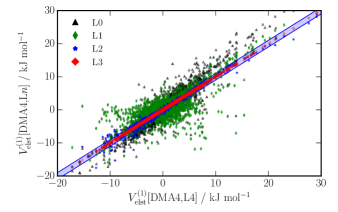
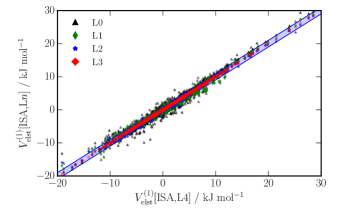
Figure 1: Scatter plot of model electrostatic energies from the DMA4 and ISA-DMA models at various ranks. The multipole expanded electrostatic energies $V^{(1)}_{\rm elst}[{\rm DM}]$ for rank $n$ models, $n=0,1,2,3$, (i.e. including multipole moments only up to rank $n$) are plotted against the energies calculated with the rank 4 model (on the $x$-axis). No damping has been used. The DMA4 results are in the top panel and the ISA-DMA (BS-ISA, $\zeta=0.1$) results are presented in the bottom panel. The blue bar represents the $\pm 1$ $\rm{kJ\,mol}^{-1}$ error range.

In fig. 7 of ref. 47 we demonstrated this aspect of the ISA-DMA moments: in contrast to the DMA4 moments, the penetration energy derived from the ISA-DMA model at rank 4 is indeed significantly more proportional to $E^{(1)}_{\rm exch}$ for the pyridine dimer. This alone makes the ISA-DMA model more appropriate for this system—or indeed, any other, as this proportionality seems to be generally true. Here we will look at the data presented in ref. 47 differently, to show more clearly how rapidly the DMA4 and ISA-DMA multipole expansions converge with rank.

For the construction of accurate electrostatic models, it is advisable to include atom charges, dipoles and quadrupoles. The dipoles are needed to describe features such as lone pairs, while quadrupoles are needed to describe $\pi$-orbital features. Octopoles and hexadecapoles can improve the description further but the improvement is not generally worth the increased computational cost of the model. However, for many applications, particularly for large molecules, due to program design limitations or more fundamentally, due to computational limitations, only charge models may be permissible. So the question arises: How do the multipole models behave when truncated to lower orders in rank? In Figure 1 we have plotted $V^{(1)}_{\rm elst}[{\rm DM}]$ calculated with each of the two multipole models with truncated rank against the same with all terms to rank 4 (deemed to be converged) included. We clearly see that while the rank 4 terms are not needed in the DMA4 model, any further truncation results in unacceptably large errors and very little correlation is left between the converged results (terms to rank 4) and those with ranks limited to 0 (charges) and 1 (charges and dipoles). In contrast, the ISA-DMA multipoles are distinctly better behaved upon truncation, with a strong correlation between all truncated models and the fully converged energies. This has some advantages: it may be possible to truncate the ISA-based distributed multipole model to much lower rank, perhaps even to rank 0, without the need to re-parametrize the potential. We shall return to this issue below.

We point out here that while the DMA4 multipole model is not directly amenable to rank truncation, there is a way to perform a rank transformation that generally does not result in significant errors. This is done using by optimizing a distributed-multipole description using the Mulfit program of Ferenczy et al.Winn et al. (1997); Ferenczy et al. (1997), in which the effects of higher-rank multipoles on each atom are represented approximately by multipoles of lower ranks on neighbouring atoms. In this way, a model including multipoles up to quadrupole can incorporate some of the effects of higher multipoles. This approach has recently been used effectively to generate simple electrostatic models for a wide range of polycyclic aromatic hydrocarbons occurring in the formation of soot.Totton et al. (2010, 2011) However the ISA-DMA treatment is consistently better.

V.2 Polarization and charge-transfer

In this paper we distinguish between the polarization energy and the induction energy. In SAPT (or SAPT(DFT)), the polarization energy and charge-transfer are combined in the induction energy. We use regularised SAPT Patkowski et al. (2001) to separate these two contributions Misquitta (2013), and by polarization energy we mean that part of the induction energy that is not associated with charge transfer.

The importance of polarizability in the interactions between polar and polarizable molecules is now well recognized Welch et al. (2008); Sebetci and Beran (2010), as is the inadequacy of the common approximation of polarization effects by the use of enhanced static dipole moments. In CamCASP we use coupled Kohn–Sham perturbation theory to obtain an accurate charge-density susceptibility, $\alpha({\mathbf{r}},{\mathbf{r}}^{\prime})$, which describes the change in charge density at ${\mathbf{r}}$ in response to a change in electrostatic potential at ${\mathbf{r}}^{\prime}$. Using a constrained density-fitting-based approach Misquitta and Stone (2006), the charge density susceptibility is partitioned between atoms to obtain a distributed-polarizability model $\alpha^{ab}_{tu}$ that gives the change in multipole $Q^{b}_{u}$ on atom $b$ in response to a change in the electrostatic potential derivative $V^{a}_{t}$ at atom $a$. Here $u=00$ for the charge, $10=z$, $11c=x$ or $11s=y$ for the dipole, $20$, $21c$, $21s$, $22c$ or $22s$ for the quadrupole components, and so on; while $t=00$ for the electrostatic potential, $10$, $11c$ or $11s$ for the components of the electrostatic field, $20$ etc. for the field gradient, and so on. Note that the electric field components are $E_{x}=E_{11c}=-V_{11c}$, $E_{y}=E_{11s}=-V_{11s}$ and $E_{z}=E_{10}=-V_{10}$.

This is a non-local model of polarizability. That is, the electric field at one atom of a molecule can induce a change in the multipole moments on other atoms of the same molecule. This is an impractical and unnecessarily complicated description that seems to be needed only for special cases such as low-dimensional extended systems Misquitta et al. (2010). For most finite systems, the moments induced on neighbouring atoms $b$ by a change in electric field on atom $a$ can be represented by multipole expansions on atom $a$, giving a local polarizability description in which the effect of a change in electric field at atom $a$ is described by changes in multipole moments on that atom alone. This is a somewhat over-simplified description of the procedure, and more detailed accounts have been given by Stone & Le SueurLe Sueur and Stone (1994), and by Lillestolen & WheatleyLillestolen and Wheatley (2007). The latter is a more elaborate approach that deals rather better with the convergence issues arising from induced moments on atoms distant from the one on which the perturbation occurs. The local polarizability model is a much more compact and useful description. In particular, the local picture removes charge-flow effects, where a difference in potential between two atoms induces a flow of charge between them. Such flows of charge still occur, but they are described in terms of local dipole polarizabilities. We point out here that the ‘self-repulsion plus local orthogonality’ (SRLO) distribution method Rob and Szalewicz (2013) can be used to eliminate the charge-flow terms altogether (for most molecules). This technique, which is a modification of the constrained density-fitting-based distribution method Misquitta and Stone (2006) is available in CamCASP but has not been used for the results of this paper. The SRLO polarizabilities are non-local and will typically need localization to be usable by most simulation programs.

The resulting localized polarizability description can be refined by the method of Williams & Stone Williams and Stone (2003) using the point-to-point responses: the change in potential at each of an array of points around the molecule in response to a point charge at any of the points. An important advantage of this method is that the final, refined polarization model can be chosen to suit the problem—for example a simple isotropic dipole–dipole model, or an elaborate model with anisotropic polarizabilities up to quadrupole–quadrupole or higher. For a given choice of model, the refinement procedure ensures that we obtain the highest accuracy (in an unbiased sense if sufficiently dense grids of point-to-point responses are used) subject to the limitations of the model. The combination of the SAPT(DFT) calculation of local (point-to-point) responses with this refinement procedure is referred to here as the WSM method Misquitta and Stone (2008); Misquitta et al. (2008).

The quality of the WSM description can be judged by the accuracy of the interaction energy of a point charge with the molecule. This interaction comprises the classical electrostatic energy of interaction of the point charge with the molecular charge distribution, and the additional term, the polarization energy, that arises from the relaxation of the molecular charge distribution in response to the point charge. These components can be separated using SAPT(DFT). The polarization energy of pyridine in the field of a point charge is mapped in the left-hand picture of Figure 2(a). We construct a grid on the vdW$\times 2$ surface of pyridine—that is, the surface made up of spheres of twice the van der Waals radius around each atom—and the polarization energy is calculated for a unit point charge at each point of the grid in turn. The remaining three maps in Figure 2(a) show the error in the polarization energy for three local polarizability descriptions: L1 uses dipole polarizabilities on each atom, L2 includes dipole–quadrupole and quadrupole–quadrupole polarizabilities, and L1,iso uses isotropic dipole polarizabilities on each atom. It is clear that the dipole-polarizability models are rather poor, and that an accurate description needs to include quadrupole polarizabilities.

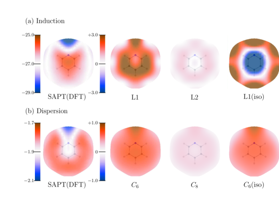
Figure 2: (a) Polarization and (b) dispersion energy maps and difference maps on the 2$\times$vdW surface of pyridine. Polarization energies have been calculated using a $+1e$ point-charge probe and dispersion energies with a neon atom probe. Energies in $\rm{kJ\,mol}^{-1}$.

V.2.1 Polarization damping

If the polarization interaction between molecules is calculated using distributed multipoles for the electrostatic potential and distributed polarizabilities for the polarization model, the effects of molecular overlap are absent and damping is needed to avoid the so-called polarization catastrophe which results in unphysical energies. In our early work on this issue Misquitta and Stone (2008) we advocated damping the classical polarization expansion to best match the total induction energies from SAPT(DFT). Through numerical simulations of the condensed phase and the work of Sebetci and Beran Sebetci and Beran (2010) we now know this to be incorrect, as it leads to excessive many-body polarization energies. The polarization damping must instead be determined by requiring that the classical polarization model energies best match the true polarization energies from SAPT(DFT) Misquitta (2013). As noted above, perturbation theories like SAPT and SAPT(DFT) do not define a true polarization energy, but rather the induction energy, which is the sum of the polarization energy and the charge-transfer energy. Recently one of us described how regularized SAPT(DFT) can be used to split the second-order induction energy into the second-order polarization and charge-transfer components Misquitta (2013) which are defined as follows:

$$E_{\rm POL}^{(2)} =E^{(2)}_{\rm IND}({\rm Reg})$$

$$E_{\rm CT}^{(2)} =E^{(2)}_{\rm IND}-E^{(2)}_{\rm IND}({\rm Reg}),$$ (14)

where $E^{(2)}_{\rm IND}({\rm Reg})$ is the regularized second-order induction energy. This definition leads to a well-defined basis limit for the second-order polarization and charge-transfer energies Misquitta (2013). We determine the damping needed for the classical polarization expansion by requiring that the non-iterated model energies best match $E_{\rm POL}^{(2)}$. Once a suitable damping has been found, an estimate for the infinite-order polarization energy $E_{\rm POL}^{(2-\infty)}$ is obtained by iterating the classical polarization model to convergence.

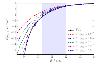
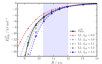
Figure 3: Second-order polarization energies vs. centre-of-mass separation $R$ for the doubly-hydrogen-bonded pyridine dimer, obtained from regularized SAPT(DFT) and from distributed polarization models. Model polarization energies are reported with local WSM models with a maximum rank of 1 (L1, top) and 2 (L2, bottom). Models are shown with a range of damping parameters using damping functions described in the text. The basin of the minimum along the radial direction is indicated by the light blue shaded region.

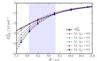
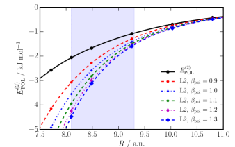
Figure 4: Second-order polarization energies vs. centre-of-mass separation $R$ for the T-shaped pyridine dimer with N pointing to the centre of the ring. See the caption of Figure 3 for a description.

In principle the above procedure gives us a straightforward way to define the damping: once the form of the damping function is chosen (we use Tang–Toennies damping in this work) all we need to do is determine the damping parameters needed by fitting to $E_{\rm POL}^{(2)}$ energies calculated for a suitable set of dimer orientations. Since the many-body polarization energy is built up from terms involving pairs of sites, we should expect that the damping parameters depend on the pairs of interacting sites, and potentially on their relative orientations. Indeed, one of us has shown Misquitta (2013) that for small dimers the damping parameters do depend quite strongly on the site types involved. A single-parameter damping model that depends only on the types of interacting molecules may be constructed, but such a model is a compromise, and must usually be determined by fitting to data biased towards the important dimer configurations only Misquitta (2013). The advantage of this approach is that the model is simpler and very few evaluations of $E_{\rm POL}^{(2)}$ are needed to determine the damping parameter, but the disadvantage is that the model is almost certainly biased towards a few dimer orientations, and additionally, these important orientations need to be known before the final potential is constructed. The last requirement—that we need to have knowledge of the potential—is not as serious as it may seem, as the choice of damping has no effect on the two-body interaction potential: this choice affects the many-body polarization energy only. So it is possible to make an informed guess for the damping parameter, determine the parameters of the intermolecular potential, and subsequently re-assess this choice by examining the performance of the polarization model at the important dimer configurations, and, if necessary, alter the model and re-fit.

The initial choice for the damping parameter in pyridine was obtained using two dimer orientations: the doubly hydrogen-bonded $C_{2h}$ dimer, and a T-shaped dimer with the nitrogen of one molecule pointing to the ring of the other. These were chosen so as to sample both H$\cdots$N and N$\cdots$C interactions, though in retrospect the latter proved to be unimportant. In Figure 3 we display the second-order polarization energies calculated using various single-parameter damping models for the $C_{2h}$ structure. Energies for only two of the three polarization models are shown, as the isotropic rank 1 (L1(iso)) model is nearly identical in behaviour to the L1 model. The optimum damping parameter for the L1 model lies between 1.2 and 1.3 a.u., while for the L2 model a stronger damping between 1.0 and 1.1 a.u. is needed. To an extent, the deficiencies of the L1 model are compensated by using a weaker damping.

The single-parameter damping approach has a serious limitation. In Figure 4 we display similar data for the T-shaped dimer orientation with the N of one molecule pointing to the centre of the ring of the other. Here we see that the polarization models need to be considerably more heavily damped with a damping coefficient of 0.9 a.u. for the L1 (and L1(iso)) model and one less than 0.9 a.u. for the L2 model. It is possible that we observe this large variation in the damping because of the strong anisotropy of the molecule, and also because a single damping coefficient is not enough. Perhaps we need to use separate damping parameters for each pair of atoms Misquitta (2013), or even to make the damping parameters orientation-dependent. As a compromise, we have chosen to use the simpler L1 model with a damping coefficient of $\beta_{\rm pol}=1.25$ a.u. This model seems capable of describing the polarization in both orientations presented here.

This approach to choosing the damping parameter remains the most problematic part of our approach to potential development. The choice of damping parameters may seem somewhat arbitrary and biased to the choice of dimer configurations used to determine the damping, but this is probably too pessimistic a view for the following reasons:

• The choice of damping does not affect the two-body interaction energy as the error in the induction energy will be absorbed in the short-range part of the potential. The damping does however alter the many-body polarization energy.

• We should regard this as an iterative process: the damping model will normally be assessed and possibly changed once we have a better understanding of the full PES. Indeed this was done in the present work. We will re-visit this issue in §LABEL:B-sec:pol-damping-revisited in Part II.

V.3 Dispersion models

In CamCASP, we normally calculate atom–atom dispersion coefficients using polarizabilities computed at imaginary frequency and localised using the WSM localization scheme. The procedure involves integrals over imaginary frequencyStone (1996), and because the imaginary-frequency polarizability is a very well-behaved function of the imaginary frequency the integrals can be carried out accurately and efficiently using Gauss-Legendre quadratureMisquitta and Stone (2008). Since the dispersion coefficients are derived from the WSM polarizability model, it is possible to choose the dispersion model to suit the problem, for example by limiting the polarizabilities to isotropic dipole–dipole, leading to an isotropic $C_{6}R^{-6}$ model, or by including all polarizabilities up to quadrupole–quadrupole, which yields a model including anisotropic dispersion terms up to $R^{-10}$. (This latter procedure omits some $R^{-10}$ terms arising from dipole–octopole polarizabilities, but they could be included too if desired.) Within the constraints of the model, the WSM polarizabilities, and hence the WSM dispersion models will be optimized to be the best in an unbiased sense. Within these constraints, intramolecular through-space polarization effects are fully or partially accounted for in the WSM models.

The dispersion energy of pyridine with a neon atom probe placed on the vdW$\times 2$ surface of pyridine is mapped in the left-hand picture of Figure 2(b). In the remaining three maps in this figure we show the error in the dispersion energy for three local dispersion models: the $C_{6}$ model includes anisotropic $C_{6}$ terms on all atoms; the $C_{8}$ model additionally includes $C_{7}$ and $C_{8}$ contributions between the heavy atoms; and the $C_{6,{\rm iso}}$ model includes only isotropic $C_{6}$ terms. The $C_{10}$ and $C_{12}$ models are not shown as they exhibit errors close to zero on the scale shown. It should be clear that to achieve a high accuracy we need to include higher-rank dispersion effects — the dispersion anisotropy is not apparently important in this system, though we may expect it to be important in larger systems. Also, the errors made by both the $C_{6}$ models are fairly uniform, and so the lack of higher-order terms in these models may be compensated for by scaling the $C_{6}$ coefficients. Indeed, we have demonstrated this in a previous publication Misquitta and Stone (2008) and will address this below.

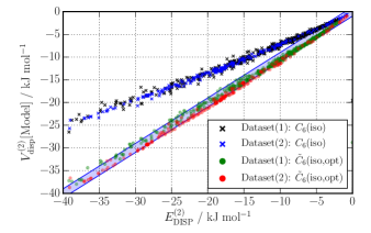
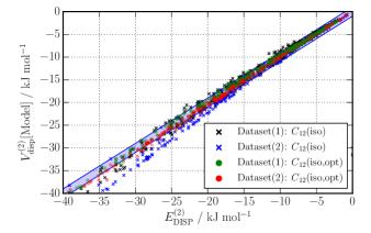
Figure 5: Scatter plot of pyridine dimer dispersion energies using various models, against reference $E^{(2)}_{\rm DISP}$ energies calculated using SAPT(DFT). See text for details. The bar represents the $\pm 1$ $\rm{kJ\,mol}^{-1}$ error range.

The WSM dispersion models described above need to be suitably damped for them to be applicable in a potential. We have used the Tang–Toennies Tang and Toennies (1984) damping functions and a single damping parameter for all pairs of sites. The damping model needs to account for two effects: First, the SAPT(DFT) dispersion energy, $E^{(2)}_{\rm DISP}$, includes the effects of penetration and exchange, which are absent from the $C_{n}R^{-n}$ expansion. Secondly, the dispersion expansion suffers from an unphysical mathematical divergence as $R\rightarrow 0$. For both reasons the models have to be damped. Damping using the Tang–Toennies functions cancels out the mathematical divergence at small $R$ and, with an appropriate damping parameter, is also able to account for the penetration and exchange effects, albeit approximately. We have opted for the simplest damping model, in which $\beta_{\rm disp}$ depends on the interacting molecules only and is given by eq. (9). With $I_{A}=I_{B}=0.3488$ a.u. we get $\beta_{\rm disp}=1.67$ a.u.

Figure 5 (bottom) shows the performance of the $C_{12}{\rm(iso)}$ isotropic dispersion models for the pyridine dimer, As can be seen from the Figure, the above damping works reasonably well for the $C_{12}{\rm(iso)}$ model with (unweighted) r.m.s. errors of $0.86$ $\rm{kJ\,mol}^{-1}$ for dispersion energies from Dataset(1) in the energy range $-40$ to $0$ $\rm{kJ\,mol}^{-1}$. However, for Dataset(2) which includes more strongly bound dimers, the model performs less well with an r.m.s. error of $2.30$ $\rm{kJ\,mol}^{-1}$ in the same energy range. The model dispersion energies are systematically overestimated for the low energy dimers, with errors as large as $4$ $\rm{kJ\,mol}^{-1}$. While these errors are just within ‘chemical accuracy’, they are too large for our purposes. They may stem from the choice of damping function, the damping parameter chosen (in particular, our use of a single, atom-pair independent isotropic damping parameter) and also the WSM dispersion coefficients. To account for some of these deficiencies, while maintaining the isotropy of the model, we have chosen to relax the dispersion coefficients in the $C_{12}{\rm(iso)}$ model. The relaxation was done using constrained optimisation with harmonic constraints in the form given by eq. (12) used to pin the dispersion coefficients to the values obtained from the WSM procedure. We used tight constraints to prevent the model parameters from taking on unphysical (negative) values. The relaxation was done using only the random dimers from Dataset(1), with the low energy dimers from Dataset(2) used to assess the quality of the relaxation. The relaxed model, $C_{12}{\rm(iso,opt)}$, is a significant improvement, with r.m.s. errors of $0.41$ $\rm{kJ\,mol}^{-1}$ on the training set of random dimers and $0.68$ $\rm{kJ\,mol}^{-1}$ on the test set of low energy dimers.

In a similar manner we have created an isotropic $C_{6}$ dispersion model for this system. From Figure 5 (top) we see that the $C_{6}{\rm(iso)}$ model systematically underestimates the second-order dispersion energy. This is to be expected, as the higher ranking dispersion contributions are significant for close dimer separations. We have previously argued Misquitta and Stone (2008) that rather than use the $C_{6}{\rm(iso)}$ model directly, we should instead use a scaled model in which all dispersion coefficients are scaled by a constant to match the reference $E^{(2)}_{\rm DISP}$ energies. Here we additionally optimise the scaled model in the manner described above. The resulting model, $\tilde{C}_{6}{\rm(iso,opt)}$ (here the tilde indicates that this is a scaled model), exhibits an r.m.s. error of $0.68$ $\rm{kJ\,mol}^{-1}$ on the training set and $1.00$ $\rm{kJ\,mol}^{-1}$ on the test set. However, such a scaled model will systematically overestimate the long-range contribution to the dispersion energy, and this is a significant drawback: while the scaled $C_{6}{\rm(iso)}$ model may be used to model small, gas-phase clusters, it is not suitable for the condensed phase because the scaling causes an excessive van der Waals pressure and the resulting structures are significantly more dense. As one of our aims is to use the resulting potentials in the study of the condensed phase, we cannot use the scaled model. However, we can simplify the $C_{12}{\rm(iso)}$ model by dropping the $R^{-12}$ terms, which contribute an insignificant amount to the dispersion energy, so we have used a $C_{10}{\rm(iso,opt)}$ model in the potentials for pyridine.

VI Short-range energy models

The short-range part of the potential comprises several effects. All of the long-range terms are modified at short range, as mentioned above. The multipole expansion on which the long-range expressions are based converges more slowly or not at all at short distances, and is incorrect when the charge densities overlap, even if it does converge. Damping can be used to correct the dispersion and polarization terms at short range, but in addition there are corrections arising from electron exchange, electrostatic penetration, and charge tunneling, or charge transfer, between the molecules.

The dominant short-range term is the exchange-repulsion: the wavefunction for two overlapping molecules cannot be treated as a simple product of isolated-molecule wavefunctions, but has to be antisymmetrized with respect to electron exchanges between the molecules. This modifies the electron distribution and results in a repulsive energy. It is straightforward to calculate the exchange-repulsion energy ab initio, but it has to be fitted by a suitable functional form for use in an analytic potential.

The electrostatic interaction is also modified by the effects of overlap. If a distributed multipole expansion is used, it will still converge at moderate overlap, but it does not converge to the non-expanded energy, $E^{(1)}_{\rm elst}$. The difference between $E^{(1)}_{\rm elst}$ and the converged multipole energy $V^{(1)}_{\rm elst}[{\rm DM}]$ is the electrostatic penetration energy, $E^{(1)}_{\rm pen}$. We have previously shown Misquitta et al. (2014) that $E^{(1)}_{\rm pen}$ is approximately proportional to the first-order exchange energy, so the two terms can, in principle, be modelled together. Alternatively a separate model for $E^{(1)}_{\rm pen}$ can be developed, possibly based on suitable damping functions Stone (2011), but we have not explored this possibility.

The contribution to the interaction energy from charge transfer — or, more appropriately, the intermolecular charge delocalisation energy — appears at second and higher orders in the perturbation expansion. Previously one of us has shown that this energy can be interpreted as an energy of stabilization due to electron tunneling Misquitta (2013), so we may expect the charge transfer energy to decay exponentially with separation. In principle, the charge transfer energy should be modelled as a separate exponentially decaying term, but as we shall see, it is approximately proportional to the first-order exchange energy and may therefore be modelled together with $E^{(1)}_{\rm exch}$.

Finally we will use the short-range potential to account for any residual differences between the multipole expansions and the reference SAPT(DFT) energies. The full form of the short-range energy, $E_{\rm sr}^{(1-\infty)}$, is shown in eq. (10) where we have also implicitly defined the first-order short-range energy, $E_{\rm sr}^{(1)}$, and the contributions from second to infinite order, $E_{\rm sr}^{(2-\infty)}$.

VI.1 Fitting the short-range potential

The short-range part of the potential has often been represented by empirical $R^{-12}$ Lennard-Jones atom–atom terms, but for accurate potentials a Born–Mayer (exponential) atom–atom form is usually preferred (eq. (11)), and it is essential in most cases to allow it to be anisotropic, since the non-spherical nature of bonded atoms can have a profound effect on the way that they pack together. Unfortunately, the parameters of the various atom–atom terms are strongly correlated, and this makes the already difficult non-linear fitting problem even more troublesome. A direct fit is generally not possible: it is hard to converge and tends to wander off into unphysical parameter space. Parameters can be forced to stay within reasonable limits, but this introduces an element of arbitrariness in the procedure.

It has however been found empirically that there is a close proportionality between the overlap of the electron densities on two atoms and the exchange–repulsion energy between them. This observation has been used to construct repulsion potentials directly from the density overlap, with varying degrees of successSoderhjelm et al. (2006). A better solution, which we adopt here, is to use the density overlap only to guide the parameters in a fitted potential function to a physically meaningful region of parameter space. Once an initial guess to the parameters has been obtained, the fit can be improved using constrained optimisation. Further, we will achieve the final fits to $E_{\rm sr}^{(1-\infty)}$ in stages, first by fitting to only $E_{\rm sr}^{(1)}$, and then by constrained relaxation to include the higher-order contributions from $E_{\rm sr}^{(2-\infty)}$.

VI.2 The density-overlap model

It is useful at this point to review the theoretical basis for the density-overlap model. In the mid-1970’s Kita, Noda & Inouye Kita et al. (1976), and later, in the early 1980’s Kim, Kim & LeeKim et al. (1981) proposed that the intermolecular repulsion energy of rare gas atoms could be modelled as

$$E^{(1)}_{\rm exch}({\mathbf{R}})\approx K\bigl{(}S_{\rho}({\mathbf{R}})\bigr{)}^{\gamma},$$ (15)

where $K$ and $\gamma$ are constants and the overlap $S_{\rho}$ of the two interacting densities $\rho^{A}$ and $\rho^{B}$ separated by generalised vector ${\mathbf{R}}$ is defined as

$$S_{\rho}({\mathbf{R}})=\int\rho^{A}({\mathbf{r}})\rho^{B}({\mathbf{r}})d{\mathbf{r}}.$$ (16)

Kita et al. had $\gamma=1$ and did not consider the possibility of varying this power, but Kim et al. observed that the constant $\gamma$ was close to, but less than, unity. This model was subsequently used by a number of groups and was successfully applied to study the interactions of polyatomic molecules, and has been investigated Mitchell and Price (2000); Soderhjelm et al. (2006) together with many other variants. Curiously, to the best of our knowledge, no one seems to have realised the reason for the success of this model, nor why the constant $\gamma$ is always less than one. Before going on to the numerical details of this model we will discuss both these issues as we will be led to a better understanding of the model and the exchange-repulsion energies.

First of all we should realise that although the exchange-repulsion and penetration energies are the short-range parts of the interaction energy, these energies result from the overlap of the density tails of the interacting densities. That is, we must consider the asymptotic form of the interacting densities for an atomic system Patil and Tang (2000):

$$\rho(r)=Cr^{2\beta}e^{-2\alpha r},$$ (17)

where, with $I$ as the vertical ionization energy, and $Z$ the atomic number, we have $\alpha=\sqrt{2I}$ and $\beta=-1+Q/\alpha$, where for an atom with nuclear charge $+Z$ and electronic charge $-N$, $Q=Z-N+1$. Both $I$ and $r$ here are in atomic units. In principle, the asymptotic form of the density overlap integral can be obtained by using this density in eq. (16), but the exact integral is not important. Instead we can use the result of Nyeland & Toennies Nyeland and Toennies (1986) who evaluated eq. (16) using only the exponential term in eq. (17) to get

$$S_{\rho}(R)=\mathcal{P}(R)e^{-2\alpha R},$$ (18)

where $\mathcal{P}(R)$ is a low-order polynomial in the internuclear separation $R$. For identical densities $\mathcal{P}(R)=(4/3)\alpha^{2}R^{2}+2\alpha R+1$, and for the more general case of different densities, the results of RosenRosen (1931) may be used to obtain a closed-form expression for $\mathcal{P}(R)$ that is now not a low order polynomial, but also includes exponential terms. Since $S_{\rho}$ is not a pure exponential, Nyeland & Toennies argue that the exchange-repulsion energy should be proportional to $S_{\rho}(R)/R^{2}$, but this assumes that the exchange-repulsion itself is a pure exponential, which is not the case.

The asymptotic form of the exchange-repulsion energy has been worked out by Smirnov & Chibisov Smirnov and Chibisov (1965) using the surface-integral approach and later, with a corrected proof, by Andreev Andreev (1973). Their result is

$$E^{(1)}_{\rm exch}=KR^{(7/2\alpha)-1}e^{-2\alpha R}$$ (19)

where $K$ is an angular momentum-dependent constant Kleinekathöfer et al. (1995). We observe that:

• The exchange-repulsion energy is not a pure exponential, as is often assumed, but is better represented as an exponential times a function of $R$. This has been empirically verified by Zemke and Stwalley (1999) using spectroscopic data for alkali diatomic molecules. Also, accurate analytic potentials for small van der Waals complexes have tended to use functional forms that include a pre-exponential polynomial term Korona et al. (1997); Misquitta et al. (2000); Bukowski et al. (1999). The prefactor function in eq. (19) is not a polynomial, but it is close to linear in $R$ for relevant values of $\alpha$ and $R$.

• The exchange-repulsion energy has an asymptotic form that is very similar to that of the density overlap, eq. (18), but the prefactor is different. Consequently we should not expect a direct proportionality between the two, and a better form of the density-overlap model might use

  $$E^{(1)}_{\rm exch}({\mathbf{R}})\approx\mathcal{K}({\mathbf{R}})S_{\rho}({\mathbf{R}}),$$ (20)

  where $\mathcal{K}({\mathbf{R}})$ is a low-order polynomial in ${\mathbf{R}}$.

• The exponents in the asymptotic forms of the density overlap and the exchange–repulsion will be the same only if the wavefunctions used to evaluate them are the same. In general this will not be the case. While the exchange–repulsion could be evaluated with electron correlation effects included, the density-overlap integrals are more typically evaluated using Hartree–Fock densities. Therefore, the $\alpha$ in the exponent of eq. (18) must be replaced by $\alpha_{\text{HF}}=(-2\epsilon_{\text{HOMO}})^{1/2}$, where $\epsilon_{\text{HOMO}}$ is the energy of the highest occupied molecular orbital from Hartree–Fock theory. In this case, there will be a better agreement between the exchange–repulsion energy and the density overlap if the exponents are made the same by raising the latter by the power $\gamma=(-I/\epsilon_{\text{HOMO}})^{1/2}$ as is done in eq. (15). Now in Hartree–Fock theory $|\epsilon_{\text{HOMO}}|\mathchar 12606\relax I$, so $\gamma$ is always less than unity, and for the helium, neon and argon dimers we obtain values between 0.99 and 0.97 in reasonable agreement with the empirical results of Kim et al..

We will now use these observations to construct models for the short-range energies.

Electron charge densities obtained from density functional theory are exact, in principle. In practice, because of the now well understood self-interaction problem with standard local and semi-local exchange-correlation functionals, they tend to be too diffuse. This can be corrected by applying a suitable asymptotic correction to the exchange-correlation potential Tozer and Handy (1998); Grüning et al. (2001). It is now usual to apply this correction in any SAPT(DFT) calculation; without it, even energies that depend on the unperturbed monomer densities, like the electrostatic energy, can be significantly in error. With the asymptotic correction, the asymptotic form of the density given by eq. (17) is enforced, and consequently $\gamma=1$ in eq. (15).

This has important consequences for multi-atom systems where we use the overlap model to partition $E^{(1)}_{\rm exch}$ into contributions from pairs of atoms. This idea goes back to the work of Mitchell & Price Mitchell and Price (2000) and begins with a partitioning of the densities into spatially localised contributions that will usually be centered on the atomic locations. If we can write

$$\rho^{A}({\mathbf{r}})=\sum_{a}\rho^{A}_{a}({\mathbf{r}}),$$ (21)

where $\rho^{A}_{a}$ is the partitioned density centered on (atomic) site $a$, and likewise for $\rho^{B}$, then from eqs. (15) and 16 we get

$$E^{(1)}_{\rm exch}({\mathbf{R}}) \approx\sum_{ab}K\int\rho^{A}_{a}({\mathbf{r}})\rho^{B}_{b}({\mathbf{r}})d{\mathbf{r}}$$

$$\approx\sum_{ab}KS_{\rho}^{ab}({\mathbf{R}}),$$ (22)

where $S_{\rho}^{ab}$ is the site–site density overlap. This expression may be generalised by introducing a site-pair dependence on $K$ as follows:

$$E^{(1)}_{\rm exch}({\mathbf{R}}) \approx\sum_{ab}K_{ab}S_{\rho}^{ab}({\mathbf{R}})=\sum_{ab}E^{(1)}_{\rm exch}[ab]({\mathbf{R}}),$$ (23)

where $E^{(1)}_{\rm exch}[ab]$ is the first-order exchange contribution assigned to site-pair $(ab)$. This is the distributed density overlap model. This is essentially the result obtained by Mitchell & Price but in their case, because of their use of electronic densities from Hartree–Fock theory, they had $\gamma\mathchar 12604\relax 1$ and so obtained an expression for the partitioning that is necessarily approximate.

There are a few important issues about the overlap model given in eq. (23):

• The model was originally formulated for the first-order exchange repulsion only, but, as the other short-range energy contributions are also roughly proportional to $E^{(1)}_{\rm exch}$, we may use the density-overlap model more generally for all of the short-range energy, $E_{\rm sr}^{(1-\infty)}$. Henceforth we will use the model in this general sense, that is, to model the short-range energy, $E_{\rm sr}$, however we may choose to define it.

• The model allows us to partition the short-range energy into terms associated with pairs of sites. With this partitioning, we may fit an analytical potential to individual site pairs rather than fit the sum of exponential terms given in eq. (11). The fit to each individual term $V_{\rm sr}[ab]$ (eq. (5)) is numerically better defined and may be achieved with relative ease.

• This is an approximation: Since the density overlap model cannot exactly model the short-range energy, we have $E_{\rm sr}({\mathbf{R}})\neq\sum_{a,b}E_{\rm sr}[ab]({\mathbf{R}})$. That is, there is a residual error that originates from the original ansatz given in eq. (15).

• Although the residual error is small compared with $E_{\rm sr}$, it needs to be accounted for to achieve an accurate fit, particularly as the error may be a non-negligible fraction of the total interaction energy, which is generally much smaller in magnitude than $E_{\rm sr}$. This may be achieved by constrained relaxation of the final short-range potential $V_{\rm sr}=\sum_{ab}V_{\rm sr}[ab]$.

VII ISA-based distributed density overlap

Formally, the distributed density overlap integrals, $S_{\rho}^{ab}({\mathbf{R}})$, defined through eqns. (21) and (23), are particularly straightforward to evaluate using the BS-ISA algorithm Misquitta et al. (2014) as this algorithm provides basis-space expansions for the atomic densities $\rho^{A}_{a}({\mathbf{r}})$. However, basis-set limitations mean that while the BS-ISA algorithm results in fairly well-defined atomic shape-functions, the atomic densities are not well described in the region of the atomic density tails, where the density can even attain small negative values. This not only leads to distributed density overlap integrals that can be negative, but also results in a relatively poor correlation between the first-order exchange energies and the density overlap integrals. This problem may be alleviated using better basis sets for the atomic expansions, but we have not as yet explored this option.

An alternative is to evaluate $S_{\rho}^{ab}({\mathbf{R}})$ using the atomic densities defined as

$$\rho^{A}_{a}({\mathbf{r}}) =\rho^{A}({\mathbf{r}})\times\frac{\tilde{w}^{a}({\mathbf{r}})}{\sum_{a^{\prime}}\tilde{w}^{a^{\prime}}({\mathbf{r}})},$$ (24)

where $\tilde{w}^{a}$ is the tail-corrected shape-function for site $a$ as defined in Ref. 47 as a piece-wise function:

$$\tilde{w}^{a}({\mathbf{r}})=\begin{cases}w^{a}({\mathbf{r}})&\text{if}\ |{\mathbf{r}}|\leq r^{a}_{0}\\ w_{\rm L}^{a}({\mathbf{r}})&\text{otherwise},\end{cases}$$ (25)

where $w^{a}({\mathbf{r}})$ is the atomic shape-function that is the spherical average of atomic density $\rho^{A}_{a}({\mathbf{r}})$, and the long-range form of the shape-function is defined as $w_{\rm L}^{a}({\mathbf{r}})=A_{a}\exp{(-\alpha_{a}|{\mathbf{r}}-{\mathbf{R}}_{a}|)}$, where $r^{a}_{0}$ is a cutoff distance, and the constants in $w_{\rm L}^{a}$ are defined to enforce continuity and charge-conservation. Misquitta et al. (2014) The shape-functions may be thought of as pro-atomic densities that encode the ionic state of the atom in its molecular environment. This ionic state is not fixed and is instead determined self-consistently through the ISA iterations Lillestolen and Wheatley (2009). While the atomic shape-functions are spherically symmetrical, the atomic densities are not. Now, the distributed density overlap integral is defined as

$$S_{\rho}^{ab}({\mathbf{R}})=\int\left(\rho^{A}({\mathbf{r}})\frac{\tilde{w}^{a}({\mathbf{r}})}{\sum_{a^{\prime}}\tilde{w}^{a^{\prime}}({\mathbf{r}})}\right)\left(\rho^{B}({\mathbf{r}})\frac{\tilde{w}^{b}({\mathbf{r}})}{\sum_{b^{\prime}}\tilde{w}^{b^{\prime}}({\mathbf{r}})}\right)d{\mathbf{r}}.$$ (26)

Due to the piece-wise nature of $\tilde{w}^{a}$, this integral must be evaluated numerically using a suitable atom-centered integration grid. Using techniques described by us earlier Misquitta et al. (2014), we evaluate the terms in eq. (26) in $\mathcal{O}(N^{0})$ computational effort. This is done by defining local neighbourhoods, $\mathcal{N}_{a}$ and $\mathcal{N}_{b}$, for sites $a$ and $b$. These neighbourhoods are based on the dimer configuration, so $\mathcal{N}_{a}$ may include sites that belong to monomer B, and vice versa for $\mathcal{N}_{b}$. The neighbourhoods are usually defined using an overlap criterion that naturally takes the basis set used into account with basis sets containing more diffuse functions resulting in larger neighbourhoods. The integration grid, and various terms in the integral $S_{\rho}^{ab}$ are then evaluated using sites in the intersection set $\mathcal{N}_{a}\cap\mathcal{N}_{b}$. This intersection set may be null for monomers that are sufficiently far apart. In this manner the density overlap integrals are calculated with linear effort.

VIII Summary

This completes the overview of the method that we have applied to the pyridine dimer in the following paper. To summarize, we have described a robust and easily implemented algorithm for developing accurate intermolecular potentials in which most of the potential parameters are derived from the charge density and density response functions. Significantly, the remaining, short-range parameters are robustly determined by associating these with specific atom pairs using a distributed density-overlap model based on a basis-space implementation of the iterative stockholder atoms (ISA) algorithm.

We have developed multipole expanded models for the electrostatic, polarization and dispersion interactions for the pyridine dimer. The electrostatic model is based on a distributed multipole analysis (DMA) that uses a density partitioning method based on the basis-space version of the iterated stockholder atoms algorithm (BS-ISA) Misquitta et al. (2014). These ISA-DMA multipoles are demonstrated to converge more rapidly with rank that the more commonly used distributed multipoles from Stone’s algorithm Stone (2005), and additionally, the ISA-DMA expansion is shown to demonstrate a systematic decrease in accuracy when truncated to lower ranks. In Part II we will probe these properties of the ISA-DMA expansion on the total interaction energy models for the pyridine dimer.

We have used regularised SAPT(DFT) Misquitta (2013) to develop a polarization models for the pyridine dimer. The L1 model includes anisotropic distributed polarizabilities and the L2 model additionally includes rank 2 terms on the heavy atoms. Both models have been damped to recover the second-order true polarization energy defined as the regularised second-order induction energy Misquitta (2013). In both cases the distributed polarizabilities have been obtained using the Williams–Stone–Misquitta (WSM) algorithm Misquitta and Stone (2006, 2008); Misquitta et al. (2008); Misquitta and Stone (2008). This algorithm has also been used to develop distributed dispersion energy models for the pyridine dimer. We have tuned these models — one with $C_{6}{\rm(iso)}$ terms only and the other including terms to $C_{12}{\rm(iso)}$ — to SAPT(DFT) total dispersion energies.

We have in addition provided an argument based on the asymptotic forms of the first-order exchange-repulsion energy and the density-overlap which provides a theoretical explanation for the success of the density-overlap model. Additionally, we have demonstrated that the power $\gamma$ used in the density overlap model should be identically $1$ if asymptotically correct densities are used. Setting $\gamma=1$ allows the density-overlap model to be distributed so as to partition the short-range energy into terms associated with pairs of sites. This distribution has been used before by other groups, but here we base it on a firm theoretical foundation. We argue that while the exponential terms in the first-order exchange energy and the density-overlap agree, the polynomial pre-factors are different, so that a better model may be achieved by allowing the model to contain a distance-dependent pre-factor.

Finally, we have provided an algorithm for a distributed density-overlap model for the short-range (repulsion) energy that used the BS-ISA density-partitioning scheme rather than the density-fitting scheme we have advocated in previous papers Stone and Misquitta (2007); Misquitta et al. (2008). In the Part II, we will demonstrate how, with this algorithm, in particular the ISA approach to atoms-in-a-molecule, a set of accurate, many-body potentials for the pyridine dimer can be derived using a relatively small number of dimer energies calculated using SAPT(DFT). Importantly, we will demonstrate how with this approach we resolve the difficulties hitherto encountered in determining the short-range parameters and the atomic shape anisotropy terms.

IX Acknowledgements

AJM would like to thank Prof Sally Price for initiating this project and supporting it in its early stages and Dr Richard Wheatley for useful discussions related to the ISA. We would like to thank Mary J. Van Vleet for useful comments on the manuscript. AJM would also like to thank Queen Mary University of London for computing resources and the Thomas Young Centre for a stimulating environment.

This work was partially funded by EPSRC grant EP/C539109/1.

Appendices

Appendix A Programs

Many of the theoretical methods described in this paper are implemented in programs available for download. Some of these, together with their main uses in the present work, are:

• CamCASP 5.9 Misquitta and Stone (2016): Calculation of WSM polarizabilities, the dispersion models, the SAPT(DFT) energies, and overlap models.

• Orient 4.8 Stone et al. (2016): Localization of the distributed polarizabilities, calculation of dimer energies using the electrostatic, polarization and dispersion models, visualization of the energy maps, and fitting to obtain the analytic atom–atom potentials.

• Dalton 2.0 Helgaker et al. (2005): DFT calculations. A patch Bukowski et al. (2008) is needed to enable Dalton 2.0 to work with CamCASP.

Appendix B CamCASP

Many of the algorithmic details of the electronic structure methods implemented in the CamCASP suite of programs have been described in previous publications. Rather than provide an exhaustive list, we will indicate those algorithms and methods of importance for potential development, as well as some numerical techniques that are particularly important for accuracy and computational efficiency.

Some of the capabilities of the CamCASP suite of programs are as follows:

• SAPT(DFT): Interaction energies to second-order can be calculated using SAPT(DFT) Misquitta and Szalewicz (2002); Misquitta et al. (2003); Misquitta and Szalewicz (2005); Misquitta et al. (2005). Infinite-order effects may be approximated using the $\delta^{\rm HF}_{\rm int}$ correction.

• Distributed multipole models: These may be evaluated using both the GDMA algorithms Stone and Alderton (1985); Stone (2005), or directly from a density-fitting-based partitioning using a variety of constraints (see the CamCASP User’s Guide for details), or from the recently implemented ISA algorithm Misquitta et al. (2014).

• Distributed frequency-dependent polarizabilities: These may be calculated in non-local form using constrained density-fitting-based partitioning schemes Misquitta and Stone (2006), which include the SRLO method Rob and Szalewicz (2013) as a special case. Localised models may be obtained using the Williams–Stone–Misquitta (WSM) model Misquitta and Stone (2008); Misquitta et al. (2008).

• Distributed dispersion models: These may be evaluated directly using the non-local frequency-dependent models Misquitta et al. (2010), or from localised polarizability models obtained using the WSM procedure Misquitta and Stone (2008). Models may be isotropic or anisotropic.

• Linear-response kernel: The code is able to evaluate the linear-response kernel using the ALDA, CHF and hybrid, ALDA+CHF, kernels. These integrals are evaluated internally.

• Interfaces: CamCASP can use molecular orbitals calculated from the Dalton program (versions from 2006 to 2015 are supported), the NWChem 6.x program and GAMESS(US) .

These are the major features of the CamCASP program, and the code additionally includes other algorithms that are important for model development. These include the ability to calculate distributed density-overlap integrals and, from these, develop density overlap models for the short-range intermolecular interaction energy, and interfaces to the Orient programStone et al. (2016) to aid in visualisation of the interaction energy models and fitting of intermolecular potentials.

References

- Podeszwa et al. (2006) Podeszwa, R.; Bukowski, R.; Szalewicz, K. J. Chem. Theory Comput. 2006, 2, 400–412.
- Hesselmann et al. (2005) Hesselmann, A.; Jansen, G.; Schütz, M. J. Chem. Phys. 2005, 122, 014103.
- Hesselmann et al. (2006) Hesselmann, A.; Jansen, G.; Schütz, M. J. Am. Chem. Soc. 2006, 128, 11730–11731.
- Podeszwa et al. (2007) Podeszwa, R.; Bukowski, R.; Rice, B. M.; Szalewicz, K. Phys. Chem. Chem. Phys. 2007, 9, 5561–9.
- Hesselmann et al. (2006) Hesselmann, A.; Jansen, G.; Schutz, M. J. Am. Chem. Soc. 2006, 128, 11730–11731.
- Fiethen et al. (2008) Fiethen, A.; Jansen, G.; Hesselmann, A.; Schutz, M. J. Am. Chem. Soc. 2008, 130, 1802–1803.
- Misquitta and Szalewicz (2002) Misquitta, A. J.; Szalewicz, K. Chem. Phys. Lett. 2002, 357, 301–306.
- Misquitta et al. (2003) Misquitta, A. J.; Jeziorski, B.; Szalewicz, K. Phys. Rev. Lett. 2003, 91, 33201.
- Misquitta and Szalewicz (2005) Misquitta, A. J.; Szalewicz, K. J. Chem. Phys. 2005, 122, 214109.
- Misquitta et al. (2005) Misquitta, A. J.; Podeszwa, R.; Jeziorski, B.; Szalewicz, K. J. Chem. Phys. 2005, 123, 214103.
- Hesselmann and Jansen (2002) Hesselmann, A.; Jansen, G. Chem. Phys. Lett. 2002, 357, 464–470.
- Hesselmann and Jansen (2002) Hesselmann, A.; Jansen, G. Chem. Phys. Lett. 2002, 362, 319–325.
- Hesselmann and Jansen (2003) Hesselmann, A.; Jansen, G. Chem. Phys. Lett. 2003, 367, 778–784.
- Hodges et al. (1997) Hodges, M. P.; Stone, A. J.; Xantheas, S. S. J. Phys. Chem. A 1997, 101, 9163–9168.
- Mas et al. (2003) Mas, E. M.; Bukowski, R.; Szalewicz, K. J. Chem. Phys. 2003, 118, 4386–4403.
- Mas et al. (2003) Mas, E. M.; Bukowski, R.; Szalewicz, K. J. Chem. Phys. 2003, 118, 4404–4413.
- Bukowski et al. (2006) Bukowski, R.; Szalewicz, K.; Groenenboom, G.; van der Avoird, A. J. Chem. Phys. 2006, 125, 044301.
- Welch et al. (2008) Welch, G. W. A.; Karamertzanis, P. G.; Misquitta, A. J.; Stone, A. J.; Price, S. L. J. Chem. Theory Comput. 2008, 4, 522–532.
- Podeszwa and Szalewicz (2007) Podeszwa, R.; Szalewicz, K. J. Chem. Phys. 2007, 126, 194101.
- Stone (2013) Stone, A. J. The Theory of Intermolecular Forces, 2nd ed.; Oxford University Press, Oxford, 2013.
- Jiang et al. (2007) Jiang, H.; Jordan, K. D.; Taylor, C. E. J. Phys. Chem. B 2007, 111, 6486–6492.
- Illingworth and Domene (2009) Illingworth, C. J.; Domene, C. Proc. R. Soc. A 2009, 465, 1701–1716.
- Bukowski et al. (1999) Bukowski, R.; Sadlej, J.; Jeziorski, B.; Jankowski, P.; Szalewicz, K.; Kucharski, S. A.; Williams, H. L.; Rice, B. M. J. Chem. Phys. 1999, 110, 3785–3803.
- Bukowski and Szalewicz (2001) Bukowski, R.; Szalewicz, K. J. Chem. Phys. 2001, 114, 9518.
- Kim et al. (2006) Kim, H.-Y.; Sofo, J. O.; Velegol, D.; Cole, M. W.; Lucas, A. A. J. Chem. Phys. 2006, 124, 074504–4.
- Korona et al. (1997) Korona, T.; Williams, H. L.; Bukowski, R.; Jeziorski, B.; Szalewicz, K. J. Chem. Phys. 1997, 106, 5109.
- Bukowski et al. (1999) Bukowski, R.; Szalewicz, K.; Chabalowski, C. J. Phys. Chem. A 1999, 103, 7322.
- Misquitta et al. (2000) Misquitta, A. J.; Bukowski, R.; Szalewicz, K. J. Chem. Phys. 2000, 112, 5308–5319.
- Vissers et al. (2005) Vissers, G. W. M.; Hesselmann, A.; Jansen, G.; Wormer, P. E. S.; van der Avoird, A. J. Chem. Phys. 2005, 122, 054306.
- Podeszwa et al. (2006) Podeszwa, P.; Bukowski, R.; Szalewicz, K. J. Phys. Chem. A 2006, 110, 10345–10354.
- Misquitta et al. (2008) Misquitta, A. J.; Welch, G. W. A.; Stone, A. J.; Price, S. L. Chem. Phys. Lett. 2008, 456, 105–109.
- Totton et al. (2010) Totton, T.; Misquitta, A. J.; Kraft, M. J. Chem. Theory Comput. 2010, 6, 683–695.
- Yu et al. (2011) Yu, K.; McDaniel, J. G.; Schmidt, J. R. J. Phys. Chem. B 2011, 115, 10054–10063.
- McDaniel and Schmidt (2013) McDaniel, J. G.; Schmidt, J. J. Phys. Chem. A 2013, 117, 2053–2066.
- Schmidt et al. (2015) Schmidt, J. R.; Yu, K.; McDaniel, J. G. Acc. Chem. Res. 2015, 48, 548–556.
- Misquitta and Stone (2016) Misquitta, A. J.; Stone, A. J. CamCASP: a program for studying intermolecular interactions and for the calculation of molecular properties in distributed form. University of Cambridge, 2016; http://www-stone.ch.cam.ac.uk/programs.html#CamCASP, Accessed: Mayy 2016.
- Jansen (2015) Jansen, G. 2015; Notation for second-order energies. Private communication.
- Jeziorska et al. (1987) Jeziorska, M.; Jeziorski, B.; Cizek, J. Int. J. Quantum Chem. 1987, 32, 149–164.
- Moszynski et al. (1996) Moszynski, R.; Heijmen, T. G. A.; Jeziorski, B. Mol. Phys. 1996, 88, 741–758.
- Stone and Misquitta (2007) Stone, A. J.; Misquitta, A. J. Int. Revs. Phys. Chem. 2007, 26, 193–222.
- Tang and Toennies (1992) Tang, K. T.; Toennies, J. P. Surf. Sci. Lett. 1992, 279, 203–206.
- Misquitta (2013) Misquitta, A. J. J. Chem. Theory Comput. 2013, 9, 5313–5326.
- Misquitta and Stone (2008) Misquitta, A. J.; Stone, A. J. J. Chem. Theory Comput. 2008, 4, 7–18.
- Stone and Alderton (1985) Stone, A. J.; Alderton, M. Mol. Phys. 1985, 56, 1047–1064.
- Stone (2005) Stone, A. J. J. Chem. Theory Comput. 2005, 1, 1128–1132.
- Lillestolen and Wheatley (2009) Lillestolen, T. C.; Wheatley, R. J. J. Chem. Phys. 2009, 131, 144101–6.
- Misquitta et al. (2014) Misquitta, A. J.; Stone, A. J.; Fazeli, F. J. Chem. Theory Comput. 2014, 10, 5405–5418.
- Misquitta and Stone (2006) Misquitta, A. J.; Stone, A. J. J. Chem. Phys. 2006, 124, 024111–14.
- Misquitta et al. (2008) Misquitta, A. J.; Stone, A. J.; Price, S. L. J. Chem. Theory Comput. 2008, 4, 19–32.
- Misquitta and Stone (2008) Misquitta, A. J.; Stone, A. J. Mol. Phys. 2008, 106, 1631 – 1643.
- Stone (2011) Stone, A. J. J. Phys. Chem. A 2011, 115, 7017–7027.
- Van Vleet et al. (2015) Van Vleet, M. J.; Misquitta, A. J.; Stone, A. J.; Schmidt, J. R. 2015, submitted.
- Shoemake (1992) Shoemake, K. In Graphics Gems III; Kirk, D., Ed.; Academic Press, 1992; pp 124–132.
- Kita et al. (1976) Kita, S.; Noda, K.; Inouye, H. J. Chem. Phys. 1976, 64, 3446–3449.
- Kim et al. (1981) Kim, Y. S.; Kim, S. K.; Lee, W. D. Chem. Phys. Lett. 1981, 80, 574–575.
- Nobeli et al. (1998) Nobeli, I.; Price, S. L.; Wheatley, R. J. Mol. Phys. 1998, 95, 525–537.
- McDaniel et al. (2012) McDaniel, J. G.; Yu, K.; Schmidt, J. R. J. Phys. Chem. C 2012, 116, 1892–1903.
- (58) Frisch, M. J.; Trucks, G. W.; Schlegel, H. B.; Scuseria, G. E.; Robb, M. A.; Cheeseman, J. R.; Montgomery, J. A., Jr.; Vreven, T.; Kudin, K. N.; Burant, J. C.; Millam, J. M.; Iyengar, S. S.; Tomasi, J.; Barone, V.; Mennucci, B.; Cossi, M.; Scalmani, G.; Rega, N.; Petersson, G. A.; Nakatsuji, H.; Hada, M.; Ehara, M.; Toyota, K.; Fukuda, R.; Hasegawa, J.; Ishida, M.; Nakajima, T.; Honda, Y.; Kitao, O.; Nakai, H.; Klene, M.; Li, X.; Knox, J. E.; Hratchian, H. P.; Cross, J. B.; Bakken, V.; Adamo, C.; Jaramillo, J.; Gomperts, R.; Stratmann, R. E.; Yazyev, O.; Austin, A. J.; Cammi, R.; Pomelli, C.; Ochterski, J. W.; Ayala, P. Y.; Morokuma, K.; Voth, G. A.; Salvador, P.; Dannenberg, J. J.; Zakrzewski, V. G.; Dapprich, S.; Daniels, A. D.; Strain, M. C.; Farkas, O.; Malick, D. K.; Rabuck, A. D.; Raghavachari, K.; Foresman, J. B.; Ortiz, J. V.; Cui, Q.; Baboul, A. G.; Clifford, S.; Cioslowski, J.; Stefanov, B. B.; Liu, G.; Liashenko, A.; Piskorz, P.; Komaromi, I.; Martin, R. L.; Fox, D. J.; Keith, T.; Al-Laham, M. A.; Peng, C. Y.; Nanayakkara, A.; Challacombe, M.; Gill, P. M. W.; Johnson, B.; Chen, W.; Wong, M. W.; Gonzalez, C.; Pople, J. A. Gaussian 03, Revision C.02. Gaussian, Inc., Wallingford, CT, 2004.
- Adamo and Barone (1999) Adamo, C.; Barone, V. J. Chem. Phys. 1999, 110, 6158–6170.
- Dunning, Jr. (1989) Dunning, Jr., T. H. J. Chem. Phys. 1989, 90, 1007–1023.
- Williams et al. (1995) Williams, H. L.; Mas, E. M.; Szalewicz, K.; Jeziorski, B. J. Chem. Phys. 1995, 103, 7374–7391.
- Woon and T. H. Dunning (1994) Woon, D. E.; T. H. Dunning, J. J. Chem. Phys. 1994, 100, 2975–2889.
- Helgaker et al. (2005) Helgaker, T.; Jensen, H. J. A.; Joergensen, P.; Olsen, J.; Ruud, K.; Aagren, H.; Auer, A.; Bak, K.; Bakken, V.; Christiansen, O.; Coriani, S.; Dahle, P.; Dalskov, E. K.; Enevoldsen, T.; Fernandez, B.; Haettig, C.; Hald, K.; Halkier, A.; Heiberg, H.; Hettema, H.; Jonsson, D.; Kirpekar, S.; Kobayashi, R.; Koch, H.; Mikkelsen, K. V.; Norman, P.; Packer, M. J.; Pedersen, T. B.; Ruden, T. A.; Sanchez, A.; Saue, T.; Sauer, S. P. A.; Schimmelpfennig, B.; Sylvester-Hvid, K. O.; Taylor, P. R.; Vahtras, O. DALTON, a molecular electronic structure program, Release 2.0. 2005; See http://www.kjemi.uio.no/software/dalton/dalton.html.
- Bukowski et al. (2008) Bukowski, R.; Cencek, W.; Jankowski, P.; Jeziorski, B.; Jeziorska, M.; Lotrich, V.; Kucharski, S.; Misquitta, A. J.; Moszynski, R.; Patkowski, K.; Podeszwa, R.; Rybak, S.; Szalewicz, K.; Williams, H.; Wheatley, R. J.; Wormer, P. E. S.; Zuchowski, P. S. SAPT2008: an ab initio program for many-body symmetry-adapted perturbation theory calculations of intermolecular interaction energies. University of Delaware and University of Warsaw, 2008; http://www.physics.udel.edu/~szalewic/, Accessed: Oct 2013.
- Tozer and Handy (1998) Tozer, D. J.; Handy, N. C. J. Chem. Phys. 1998, 109, 10180–10189.
- Weigend et al. (1998) Weigend, F.; Haser, M.; Patzelt, H.; Ahlrichs, R. Chem. Phys. Lett. 1998, 294, 143–152.
- Weigend et al. (2002) Weigend, F.; Kohn, A.; Hattig, C. J. Chem. Phys. 2002, 116, 3175–3183.
- Akin-Ojo et al. (2003) Akin-Ojo, O.; Bukowski, R.; Szalewicz, K. J. Chem. Phys. 2003, 119, 8379–8396.
- Perdew and Wang (1992) Perdew, J. P.; Wang, Y. Phys. Rev. B 1992, 45, 13244–13249.
- Sadlej (1988) Sadlej, A. J. Coll. Czech Chem. Commun. 1988, 53, 1995–2016.
- Jeziorski and Szalewicz (2002) Jeziorski, B.; Szalewicz, K. In Handbook of Molecular Physics and Quantum Chemistry; Wilson, S., Ed.; Wiley, 2002; Vol. 8; Chapter 8, pp 37–83.
- Winn et al. (1997) Winn, P. J.; Ferenczy, G. G.; Reynolds, C. A. J. Phys. Chem. A 1997, 101, 5437–5445.
- Ferenczy et al. (1997) Ferenczy, G. G.; Winn, P. J.; Reynolds, C. A. J. Phys. Chem. A 1997, 101, 5446–5455.
- Totton et al. (2011) Totton, T.; Misquitta, A. J.; Kraft, M. Chem. Phys. Lett. 2011, 510, 154–160.
- Patkowski et al. (2001) Patkowski, K.; Jeziorski, B.; Szalewicz, K. J. Mol. Struct. (Theochem) 2001, 547, 293–307.
- Sebetci and Beran (2010) Sebetci, A.; Beran, G. J. O. J. Chem. Theory Comput. 2010, 6, 155–167.
- Misquitta et al. (2010) Misquitta, A. J.; Spencer, J.; Stone, A. J.; Alavi, A. Phys. Rev. B 2010, 82, 075312–7.
- Le Sueur and Stone (1994) Le Sueur, C. R.; Stone, A. J. Mol. Phys. 1994, 83, 293–308.
- Lillestolen and Wheatley (2007) Lillestolen, T. C.; Wheatley, R. J. J. Phys. Chem. A 2007, 111, 11141–11146.
- Rob and Szalewicz (2013) Rob, F.; Szalewicz, K. Chem. Phys. Lett. 2013, 572, 146–149.
- Williams and Stone (2003) Williams, G. J.; Stone, A. J. J. Chem. Phys. 2003, 119, 4620–4628.
- Stone (1996) Stone, A. J. The Theory of Intermolecular Forces; International Series of Monographs in Chemistry; Clarendon Press: Oxford, 1996.
- Tang and Toennies (1984) Tang, K. T.; Toennies, J. P. J. Chem. Phys. 1984, 80, 3726–3741.
- Soderhjelm et al. (2006) Soderhjelm, P.; Karlstrom, G.; Ryde, U. J. Chem. Phys. 2006, 124, 244101–10.
- Mitchell and Price (2000) Mitchell, J. B. O.; Price, S. L. J. Phys. Chem. A 2000, 104, 10958–10971.
- Patil and Tang (2000) Patil, S. H.; Tang, K. T. In Asymptotic methods in quantum mechanics; Scäfer, F. P., Toennies, J. P., Zinth, W., Eds.; Springer, 2000.
- Nyeland and Toennies (1986) Nyeland, C.; Toennies, J. P. Chem. Phys. Lett. 1986, 127, 172–177.
- Rosen (1931) Rosen, N. Phys. Rev. 1931, 38, 255–276.
- Smirnov and Chibisov (1965) Smirnov, B. M.; Chibisov, M. I. Sov. Phys.-JETP 1965, 21, 624.
- Andreev (1973) Andreev, E. A. Theor. Chim. Acta 1973, 28, 235–239.
- Kleinekathöfer et al. (1995) Kleinekathöfer, U.; Tang, K. T.; Toennies, J. P.; Yiu, C. L. J. Chem. Phys. 1995, 103, 6617–.
- Zemke and Stwalley (1999) Zemke, W. T.; Stwalley, W. C. J. Chem. Phys. 1999, 111, 4962–4965.
- Grüning et al. (2001) Grüning, M.; Gritsenko, O. V.; van Gisbergen, S. J. A.; Baerends, E. J. J. Chem. Phys. 2001, 114, 652–660.
- Stone et al. (2016) Stone, A. J.; Dullweber, A.; Engkvist, O.; Fraschini, E.; Hodges, M. P.; Meredith, A. W.; Nutt, D. R.; Popelier, P. L. A.; Wales, D. J. ORIENT: a program for studying interactions between molecules, version 4.8. University of Cambridge, 2016; http://www-stone.ch.cam.ac.uk/programs.html#Orient, Accessed: May 2016.