Modeling and Querying Data Cubes on the Semantic Web

Abstract

The web is changing the way in which data warehouses are designed, used, and queried. With the advent of initiatives such as Open Data and Open Government, organizations want to share their multidimensional data cubes and make them available to be queried online. The RDF data cube vocabulary (QB), the W3C standard to publish statistical data in RDF, presents several limitations to fully support the multidimensional model. The QB4OLAP vocabulary extends QB to overcome these limitations, allowing to implement the typical OLAP operations, such as rollup, slice, dice, and drill-across using standard SPARQL queries. In this paper we introduce a formal data model where the main object is the data cube, and define OLAP operations using this model, independent of the underlying representation of the cube. We show then that a cube expressed using our model can be represented using the QB4OLAP vocabulary, and finally we provide a SPARQL implementation of OLAP operations over data cubes in QB4OLAP.

1 Introduction

On-Line Analytical Processing (OLAP) is a well-established approach for data analysis to support decision making, that typically relates to Data Warehouse (DW) systems. It is based on the multidimensional (MD) model which views data in an $n$-dimensional space, usually called a data cube. There is a large number of MD models in the literature [9, 12, 20], based on the data cube metaphor. Historically, DW and OLAP have been used as techniques for data analysis within an organization, using mostly commercial tools with proprietary formats. However, initiatives like Open Data and Open Government are pushing organizations to publish MD data using standards and non-proprietary formats. Although several open source platforms for business intelligence (BI) have emerged in the last decade, an open format to publish and share cubes among organizations is still missing. The Linked Data [11] initiative promotes sharing and reusing data on the web using semantic web (SW) standards and domain ontologies expressed in the Resource Description Framework(RDF) (the basic data representation layer for the SW) [15], or in languages built on top of RDF (e.g., RDF-Schema [4]).

The need for tools and techniques allowing to publish and sharing data cubes did not take long to arise. Statistical data sets are usually published using the RDF Data Cube Vocabulary[6] (also denoted QB), the current W3C standard. However, as we discussed in [7, 8], the QB vocabulary does not support dimension hierarchies and aggregate functions needed for OLAP analysis. To address this challenge, we proposed a new vocabulary called QB4OLAP [8], that allows reusing data already published in QB just by adding the needed MD schema semantics (e.g., the hierarchical structure of the dimensions) and the corresponding instances that populate the dimension levels. Once a data cube is published using QB4OLAP, users are able to operate over it, not only through queries written in SPARQL [18] (the standard query language for RDF), but also using a high-level declarative OLAP language built taking advantage of the QB4OLAP metadata.

In this paper we extend our previous work, presenting a formal data model for data cubes, and we use it to provide the semantics of a set of high-level OLAP operators over data cubes. We then show that a data cube represented using this model can be represented on the semantic web using the QB4OLAP vocabulary. Finally, we provide a SPARQL implementation of the OLAP operators over QB4OLAP.

To put the reader in context, we next present the basic concepts on OLAP and SW data models.

1.1 RDF and the Semantic Web

Resource Description Framework (RDF) is a data model for expressing assertions over resources identified by an internationalized resource identifier (IRI). Assertions are expressed as triples of the form $(subject,predicate,object)$. A set of RDF triples or RDF data set, can be seen as a directed graph where the subject and object are nodes, and the predicates are arcs. Data values in RDF are called literals. Blank nodes are used to represent anonymous resources or resources without an IRI, typically with a structural function, e.g., to group a set of statements. Subjects are always resources or blank nodes, predicates are always resources, and object could be resources, blank nodes or literals. A set of reserved words defined in RDF Schema (called the rdfs-vocabulary)[4] is used to define classes, properties, and to represent hierarchical relationships between them. For example, the triple (s, rdf:type, c) explicitly states that s is an instance of c instance. Many formats for RDF serialization exist. In this paper we use Turtle [3].

SPARQL 1.1 [18] is the current W3C standard query language for RDF. Its query evaluation mechanism is based on subgraph matching: RDF triples are interpreted as nodes and edges of directed graphs, and the query graph is matched to the data graph, instantiating the variables in the query. The selection criteria is expressed using a graph pattern in the WHERE clause. Relevant to OLAP queries, SPARQL supports aggregate functions and the GROUP BY clause.

1.2 OLAP

Data Warehouses (DW) integrate data from multiple sources, also keeping their history for analysis and decision support. DWs represent data according to dimensions and facts. The former reflect the perspectives from which data are viewed, and we may have several of them. The latter corresponds to (usually) quantitative data (also known as measures) associated with different dimensions. Dimensions organize elements, or members, in hierarchies, where each element belongs to a category (or level) in a hierarchy. These are the main components of the multidimensional model, which represents facts in an $n$-dimensional space, usually called a data cube, whose axes are the dimensions, and whose cells contain the values for the measures.

Online Analytical Processing (OLAP) is the process of querying a data cube, where facts can be aggregated and disaggregated via operations called roll-up and drill-down, respectively, and filtered through slice and dice, among other operations.

As an illustration, the facts related to the sales of a company may be associated with the dimensions Time and Location, representing the sales at certain locations in certain periods of time. Assuming that facts (sales) are recorded at granularities month and city in dimensions Time and Location, respectively, a point in this space could be (January 2014, Buenos Aires), and the measure in this cell indicates the amount of the sales in January 2014, at the Buenos Aires branch. A roll-up operation over dimension Time up to level year would produce the yearly amount of sales for each city.

1.3 Problem Statement and Contributions

Ciferri et al. [5] have shown that, opposite to the usual belief, most of the multidimensional data models in the literature are at the logical level rather than at a conceptual level, and that the data cube is far from being the focus of these models. Therefore, the authors sketched (quite informally) a model and algebra where the data cube is a first-class citizen. Along the same lines, Gómez el al. [10] showed that such a model can be used to seamlessly query many kinds of multidimensional data (e.g., discrete and continuous geographic data). We follow these lines of thought, and, as our first contribution, formalize a data model where the main object is the data cube over which a conceptual query language where the operators manipulate the data cube, can be defined. This way, the user just queries data cubes, independently of the underlying data representation. Moreover, in our data model, the semantics of these operators is clearly defined using the notion of a lattice of cuboids, which is later used for query processing and rewriting. As a second contribution we show that a data cube represented using our data model can be published on the semantic web using the QB4OLAP vocabulary. Finally, as a third contribution, taking advantage of the structural metadata provided by the QB4OLAP representation, we present algorithms that produce a SPARQL implementation of the main OLAP operators over QB4OLAP data cubes. That is, an OLAP user would not need to have any knowledge of SPARQL at all, and still be able to query cubes over the semantic web.

The remainder of this paper is organized as follows. Section 2 introduces our running example. Section 3 presents a formal data model for data cubes. Then, Section 4 describes the representation of data cubes in QB4OLAP. Section 5 introduces a high-level OLAP query language purely based on operations over a data cube, and presents a set of algorithms to produce a SPARQL implementation of these operations over QB4OLAP data cubes. Finally, Section 6 discusses related work, and Section 7 concludes the paper.

2 Running Example

Throughout this paper we will be using an example based on statistical data about asylum applications to countries in the European Union, provided by Eurostat. This dataset contains information about the number of asylum applicants by month, age, sex, citizenship, and country that receives the application. It is published using QB in the Eurostat - Linked Data dataspace. Basically, a QB dataset is composed of a set of observations that represent data instances that adhere to a schema, represented by a data structure definition (DSD). However, QB lacks of the capability to represent dimension aggregation hierarchies. To allow OLAP operations, QB4OLAP allows building cube schemas on top of the observations already published using QB. In this way, the cost of adding OLAP capabilities to existing datasets is the cost of building the new dimension schema (the analysis dimensions), and populating its instances. In this example we built simple dimension hierarchies to organize countries into continents, and months into years.

Figure 1 shows the conceptual schema of the data cube (extended with hierarchies), using the MultiDim notation [19]. The asylum_applications cube has a measure (#applications) that represents the number of applications. This measure can be analyzed according to six dimensions: the sex of the applicant, age which organizes applicants according to their age group, time which represents the time of the application and consists of two levels (month and year), application_type that represents if the applicant is a first-time applicant or a returning applicant, and a geographical dimension that organizes countries into continents (Geography hierarchy) or according to its government type (Government hierarchy). This geographical dimension participates in the cube with two different roles: as the citizenship of the asylum applicant, and as the destination country of the application.

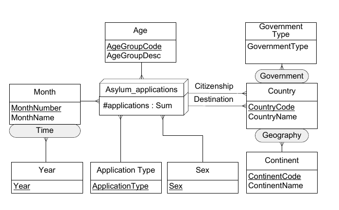
Figure 1: Conceptual schema of the Asylum Applications cube

3 Data Cubes

In multidimensional models, data are organized as cubes whose axes are dimensions. Each point in this multidimensional space is mapped into one or more spaces of measures. Dimensions are organized in hierarchies that allow analysis at different aggregation levels. The values in a dimension level are called members, and may have properties or attributes. Members in a level must have a corresponding member in the upper level in the hierarchy, and this correspondence is defined through so-called rollup functions. In this section we present a formal model for data cubes upon which we build our query language.

3.1 Data Cubes Formalization

Definition 3.1.

(Dimension schema). A dimension
schema is a tuple $\langle\mathsf{nD},\mathcal{L},\rightarrow,\mathcal{H}\rangle$ where: (a) nD is the name of the dimension; (b) $\mathcal{L}$ is a set of tuples $\langle\mathsf{name}_{l},\mathsf{A}_{l}\rangle$, called levels, where $\mathsf{name}_{l}$ identifies a level in $\mathcal{L}$, and $\mathsf{A}_{l}=\langle a_{1},\dots,a_{n}\rangle$ is a tuple of level attributes. Each attribute $a_{i}$ has a domain $Dom(a_{i})$ with $1\leq i\leq n$; (c) $(\mathcal{L},\rightarrow)$ represents a lattice with a unique bottom level and a unique top level (All), where ‘$\rightarrow$’ is a partial order that defines a parent-child relation between pairs of levels in $\mathcal{L}$; (d) $\mathcal{H}$ is a set of tuples $\langle\mathsf{name}_{h},\mathsf{L}_{h}\rangle$, called hierarchies, where $\mathsf{name}_{h}$ identifies the hierarchy, and $\mathsf{L}_{h}\subseteq\mathcal{L}$ is the set of levels that participate in the hierarchy.∎

Remark 1.

All levels in a dimension schema must belong to at least one hierarchy. For each dimension $\mathsf{nD}$ with schema $\langle\mathsf{nD},\mathcal{L},\rightarrow,\mathcal{H}\rangle$, where $\mathcal{H}=\{\langle\mathsf{h}_{1},\mathsf{L}_{h_{1}}\rangle,\dots,\langle\mathsf{h}_{i},\mathsf{L}_{h_{i}}\rangle\}$, then $\bigcup_{j=0}^{j=i}\mathsf{L}_{h_{j}}=\mathcal{L}$.

In addition, all the dimensions contain at least one default hierarchy $\langle\mathsf{name}_{h},\mathsf{L}_{h}\rangle$, with $\mathsf{L}_{h}=\mathcal{L}$. ∎

Example 3.1.

(Citizenship dimension schema) The schema of the Citizenship dimension in Figure 1 is defined as:
$\langle\mathsf{Citizenship}$ $\mathcal{L}=\{\langle\mathsf{Country},\langle\mathsf{countryCode},\mathsf{countryName}\rangle\rangle,$
$\langle\mathsf{Continent},\langle\mathsf{continentCode},\mathsf{continentName}\rangle\rangle,$
$\langle\mathsf{GovernmentType},\langle\mathsf{governmentType}\rangle\rangle,$
$\langle\mathsf{All},\langle\mathsf{all}\rangle\rangle\}$;
$\mbox{`}\rightarrow\mbox{'}=\{\mathsf{Country}\rightarrow\mathsf{Continent},\mathsf{Country}\rightarrow\mathsf{GovernmentType},$
$\mathsf{Continent}\rightarrow\mathsf{All},\mathsf{GovernmentType}\rightarrow\mathsf{All}\};$
$\mathcal{H}=\{\langle\mathsf{Geography},\{\mathsf{Country},\mathsf{Continent},\mathsf{All}\}\rangle,$
$\langle\mathsf{Government},\{\mathsf{Country},\mathsf{GovernmentType},\mathsf{All}\}\rangle\}$
∎

Definition 3.2.

(Dimension instance). A dimension instance for a dimension schema $\langle\mathsf{nD},\mathcal{L},\rightarrow,\mathcal{H}\rangle$ is a tuple $\langle\langle\mathsf{nD},\mathcal{L},\rightarrow,\mathcal{H}\rangle,\mathcal{T}_{L},\mathcal{R}\rangle$ where: (a) $\mathcal{T}_{L}$ is a finite set of tuples of the form $\langle v_{1},v_{2},\dots,v_{n_{l}}\rangle~{}\forall\mathsf{L}=\langle\mathsf{L},\langle a_{1},\dots,a_{n}\rangle\rangle\in\mathcal{L}$ such that $\forall i,i=1,\dots,n,v_{i}\in Dom(a_{i})$; (b) $\mathcal{R}$ is a finite set of relations $\mathsf{RUP}^{\mathsf{L}_{j}}_{\mathsf{L}_{i}},\mathsf{L}_{i},\mathsf{L}_{j}\in\mathcal{L}$, such that $\mathsf{L}_{i}\rightarrow\mathsf{L}_{j}~{}\in~{}\mathcal{L},\rightarrow)$. Each relation $\mathsf{RUP}^{\mathsf{L}_{j}}_{\mathsf{L}_{i}}$ relates members of $\mathsf{L}_{i}$ (child level) with members of $\mathsf{L}_{j}$ (parent level). ∎

Example 3.2.

(Citizenship dimension instance) A possible instance of the Citizenship dimension in Figure 1 is:
$\mathcal{T}_{\mathsf{Country}}=\{\langle$ ’AD’, ’Andorra’ $\rangle,\dots,\langle$’ZW’, ’Zimbabwe’$\rangle\}$
$\mathcal{T}_{\mathsf{Continent}}=\{\langle$’AF’, ’Africa’$\rangle,\dots,\langle$’OC’, ’Oceania’$\rangle\}$
$\mathcal{T}_{\mathsf{GovernmentType}}=\{\langle$’Republic’$\rangle,\dots,\langle$’Unitary state’$\rangle\}$
$\mathcal{T}_{\mathsf{All}}=\{\langle$ ’all’$\rangle\}$
$\mathcal{R}=\{\mathsf{RUP}_{\mathsf{Country}}^{\mathsf{Continent}},\mathsf{RUP}_{\mathsf{Continent}}^{\mathsf{All}},$ $\mathsf{RUP}_{\mathsf{Country}}^{\mathsf{GovernmentType}},\\ \mathsf{RUP}_{\mathsf{GovernmentType}}^{\mathsf{All}}\}$, with $\mathsf{RUP}_{\mathsf{Country}}^{\mathsf{Continent}}=\{(\langle$ ’AD’, ’Andorra’$\rangle$, $\langle$’EU’, ’Europe’$\rangle),\ldots,$ $(\langle$ ’ZW’, ’Zimbabwe’$\rangle$, $\langle$’AF’, ’Africa’$\rangle)\};$ $\mathsf{RUP}_{\mathsf{Country}}^{\mathsf{GovernmentType}}=\{(\langle$ ’AD’, ’Andorra’$\rangle$, $\langle$’Unitary state’$\rangle),\ldots,$ $(\langle$ ’ZW’, ’Zimbabwe’$\rangle$, $\langle$’Presidential system’$\rangle)\}$;
$\mathsf{RUP}_{\mathsf{Continent}}^{\mathsf{All}}=\{(\langle x\rangle$, $\langle$all$\rangle)\ |x\in\mathcal{T}_{\mathsf{All}}\}$;
$\mathsf{RUP}_{\mathsf{GovernmentType}}^{\mathsf{All}}=\{(\langle x\rangle$, $\langle$all$\rangle)\ |x\in\mathcal{T}_{\mathsf{All}}\}.$
∎

Definition 3.3.

(Cube schema). A cube schema is a tuple $\langle\mathsf{nC},\mathcal{D},\mathcal{M},\mathcal{F}\rangle$ where: (a) $\mathsf{nC}$ is the name of the cube; (b) $\mathcal{D}$ is a finite set of dimension schemas (see Def. 3.1); (c) $\mathcal{M}$ is a finite set of attributes, where each $m\in\mathcal{M}$, called measure, has domain $Dom(m)$; (d) $\mathcal{F}:\mathcal{M}\rightarrow\mathcal{A}$ is a function that maps each measure in $\mathcal{M}$ to an aggregate function in $\mathcal{A}$. ∎

Example 3.3.

(Asylum_application cube schema) We define the cube schema, presented in Figure 1 as:
$\langle$ Asylum_application, {Sex,Age,Time,Application_type,
Citizenship, Destination}, {#applications},
{#applications,Sum} $\rangle$, where dimension Citizenship is defined as in Example 3.1. We omit the definition of the other dimensions, for the sake of brevity and to avoid redundancy. ∎

To define a cube instance we need to introduce the notion of cuboid.

Definition 3.4.

(Cuboid instance). Given: (a) a cube schema $\langle\mathsf{nC},\mathcal{D},\mathcal{M},\mathcal{F}\rangle$, where $|\mathcal{D}|=D$ and $|\mathcal{M}|=M$, (b) a dimension instance $\mathsf{I}_{i}$ for each $\mathsf{D}_{i}\in\mathcal{D},\forall i,i=1,\dots,D$, and (c) a set of levels $\mathcal{V}_{Cb}=\{l_{1},l_{2},\dots,l_{D}\}$ where $l_{i}\in\mathcal{L}_{i}$ of $\mathsf{D}_{i}\in\mathcal{D},\forall i,i=1,\dots,D$, such that there are not two levels belonging to the same dimension, a cuboid instance Cb is a partial function $\mathsf{Cb}:\mathcal{T}_{l_{1}}\times\dots\times\mathcal{T}_{l_{D}}\rightarrow Dom(m_{1})\times\dots\times Dom(m_{M})$, where $m_{k}\in\mathcal{M},\forall k,k=1,\dots,M$. The elements in the domain of Cb are called cells, and $\mathcal{V}_{Cb}$ it the set of levels of the cuboid. ∎

Example 3.4.

(Cuboid instance) Consider the cube schema Asylum_application defined in Example 3.3. A possible instance of the cuboid $\mathsf{Cb}_{1}$, where $\mathcal{V}_{\mathsf{Cb}_{1}}=${Sex, Age, Month, Application_type, Country, Country$\}$ is presented in Figure 2, using a tabular representation, where the first row lists the dimensions in the cuboid, and the second row lists the dimension level corresponding to the cuboid. ∎

Figure 2: Tabular representation of a cuboid instance of the Asylum_application cube schema

Sex	Age	Time	Application_type	Citizenship	Destination	Measures
Sex	Age	Month	Application_type	Country	Country	#applications
M	14 to 17	201301, January 2013	new applicant	CM, Cameroon	BE, Belgium	5
F	less than 14	201303, March 2013	new applicant	CM, Cameroon	FR, France	5
M	18 to 34	201301, January 2013	new applicant	CM, Cameroon	FR, France	10
F	18 to 34	201301, January 2013	new applicant	CD, Democratic Republic of the Congo	BE, Belgium	25
F	18 to 34	201303, March 2013	new applicant	CD, Democratic Republic of the Congo	BE, Belgium	30

Figure 3: Two cuboid instances of the Asylum_application cube schema

Sex	Age	Time	Application_type	Citizenship	Destination	Measures
Sex	Age	Year	Application_type	Continent	Country	#applications
M	14 to 17	2013	new applicant	AF, Africa	BE, Belgium	5
F	less than 14	2013	new applicant	AF, Africa	FR, France	5
M	18 to 34	2013	new applicant	AF, Africa	FR, France	10
F	18 to 34	2013	new applicant	AF, Africa	BE, Belgium	55

(a) Cuboid $\mathsf{Cb}_{2}$

Sex	Age	Time	Application_type	Citizenship	Destination	Measures
All	Age	Year	Application_type	Continent	Country	#applications
all	14 to 17	2013	new applicant	AF, Africa	BE, Belgium	5
all	less than 14	2013	new applicant	AF, Africa	FR, France	5
all	18 to 34	2013	new applicant	AF, Africa	FR, France	10
all	18 to 34	2013	new applicant	AF, Africa	BE, Belgium	55

(b) Cuboid $\mathsf{Cb}_{3}$

The sets of the cuboid instances that refer to the same cube schema, can be organized using the concepts of adjacent cuboids and order between cuboids, defined as follows.

Definition 3.5.

(Adjacent Cuboids). Two cuboids $\mathsf{Cb}_{1}$ and $\mathsf{Cb}_{2}$, that refer to the same cube schema, are adjacent if their corresponding level sets $\mathcal{V}_{Cb_{1}}$ and $\mathcal{V}_{Cb_{2}}$ differ in exactly one level, i.e., $|\mathcal{V}_{Cb_{1}}-\mathcal{V}_{Cb_{2}}|=|\mathcal{V}_{Cb_{2}}-\mathcal{V}_{Cb_{1}}|=1$. ∎

Example 3.5.

(Adjacent cuboids) Consider the cube schema defined in Example 3.3 and the cuboids $\mathsf{Cb}_{1},\mathsf{Cb}_{2}$, and $\mathsf{Cb}_{3}$ given by $\mathcal{V}_{\mathsf{Cb}_{1}}=${Sex, Age, Month, Application_type, Country, Country$\}$, $\mathcal{V}_{\mathsf{Cb}_{2}}=${Sex, Age, Year, Application_type, Country,Country$\}$ and $\mathcal{V}_{\mathsf{Cb}_{3}}=${Sex, Age, Year, Application_type, Country, Continent$\}$. According to Definition 3.5, $\mathsf{Cb}_{1}$ is adjacent to $\mathsf{Cb}_{2}$, and $\mathsf{Cb}_{2}$ is adjacent to $\mathsf{Cb}_{3}$, but $\mathsf{Cb}_{1}$ is not adjacent to $\mathsf{Cb}_{3}$. ∎

Definition 3.6.

(Order between Adjacent Cuboids).
Given two adjacent cuboids $\mathsf{Cb}_{1}$ and $\mathsf{Cb}_{2}$, such that $\mathcal{V}_{Cb_{1}}-\mathcal{V}_{Cb_{2}}=\{l_{c}\}$ and $\mathcal{V}_{Cb_{2}}-\mathcal{V}_{Cb_{1}}=\{l_{p}\}$, and $l_{p}$ and $l_{c}$ are levels of the lattice $(\mathcal{L},\rightarrow)$ of the dimension $D_{k}$ such that $l_{c}\rightarrow l_{p}$, then $\mathsf{Cb}_{1}\preceq\mathsf{Cb}_{2}$.
Moreover, for each pair of adjacent cuboids $\mathsf{Cb}_{1}\preceq\mathsf{Cb}_{2}$ each cell $c=(c_{1},\dots,c_{k-1},c_{k},c_{k+1},\dots,c_{n},m_{1},m_{2},\dots m_{s})\in\mathsf{Cb}_{2}$ can be obtained from the cells in $\mathsf{Cb}_{1}$ as follows.
Let $(c_{1},\dots,c_{k-1},b_{k1},c_{k+1},\dots,c_{n},m_{1,1},m_{2,1},\dots m_{s,1})$ ,
$(c_{1},\dots,c_{k-1},b_{k2},c_{k+1},\dots,c_{n},m_{1,2},m_{2,2},\dots m_{s,2})$,
$(c_{1},\dots,c_{k-1},b_{kp},c_{k+1},\dots,c_{n},m_{1,p},m_{2,p},\dots m_{s,p})$ be cells in $\mathsf{Cb}_{1}$ where $(b_{k_{i}},c_{k})\in RUP_{l_{k_{c}}}^{l{k_{p}}},i=1\dots q$, that means that all members $b_{k_{i}}$ in level $l_{k_{c}}$ in dimension $D_{k}$ are in a parent-child relation with the element $c_{k}$ in level $l_{k_{p}}$ in that dimension, and the measures in cell $c\in\mathsf{Cb}_{2}$ are obtained as $m_{i}=AGG_{i}(m_{i,1},\dots,m_{i,j})$, where $AGG_{i}$ is the aggregation function related to measure $m_{i}$. ∎

Example 3.6.

(Order between cuboids) Consider the cuboids $\mathsf{Cb}_{1},\mathsf{Cb}_{2}$, and $\mathsf{Cb}_{3}$ in Example 3.5. Then $\mathsf{Cb}_{1}\preceq\mathsf{Cb}_{2}$, because Month $\rightarrow$ Year holds, and $\mathsf{Cb}_{2}\preceq\mathsf{Cb}_{3}$, because Country $\rightarrow$ Continent holds. ∎

Finally we define a cube instance as the lattice of all possible cuboids that share the same cube schema.

Definition 3.7.

(Cube Instance). Given a cube schema
$\langle\mathsf{nC},\mathcal{D},\mathcal{M},\mathcal{F}\rangle$, where $|\mathcal{D}|=D$ and $|\mathcal{M}|=M$, and a dimension instance $I_{i}$ for each $D_{i}\in\mathcal{D},i=1,\dots,D$, a cube instance $\mathsf{CI}$ is the lattice $\{\mathsf{CB},\preceq\}$ where CB is the set of all possible cuboids, and $\preceq$ is the order between adjacent cuboids in CB. ∎

Example 3.7.

(Cuboids of Asylum_application) Consider the cube schema defined in Example 3.3. All possible combinations of the levels in the six dimensions of the cube, lead to 216 cuboids, which are organized in a lattice. Assuming the instance of cuboid $\mathsf{Cb}_{1}$ in Figure 2, Figures 4a and 4b present tabular representations of instances of cuboids $\mathsf{Cb}_{2}$, and $\mathsf{Cb}_{3}$ given by $\mathcal{V}_{\mathsf{Cb}_{2}}=${Sex, Age, Year, Application_type, Continent, Country$\}$, and $\mathcal{V}_{\mathsf{Cb}_{3}}=${All, Age, Year, Application_type, Continent,Country$\}$. ∎

4 QB4OLAP and Data Cubes

In this section we first present QB4OLAP distinctive features, and then we describe in detail how the formal model defined in Section 3 can be represented in QB4OLAP.

4.1 QB4OLAP

QB4OLAP extends QB with a set of RDF terms that allow representing the most common features of the MD model. Figure 4 depicts the QB4OLAP vocabulary. Original QB terms are prefixed with “qb:”, while QB4OLAP terms are prefixed with “qb4o:” and displayed in gray background. Capitalized terms represent RDF classes, non-capitalized terms represent RDF properties, and capitalized terms in italics represent class instances. An arrow from class $A$ to class $B$, labeled $rel$ means that $rel$ is an RDF property with domain $A$ and range $B$. White triangles represent sub-class or sub-property relationships. Black diamonds represent rdf:type relationships (instances). The range of a property can also be denoted using “:”.

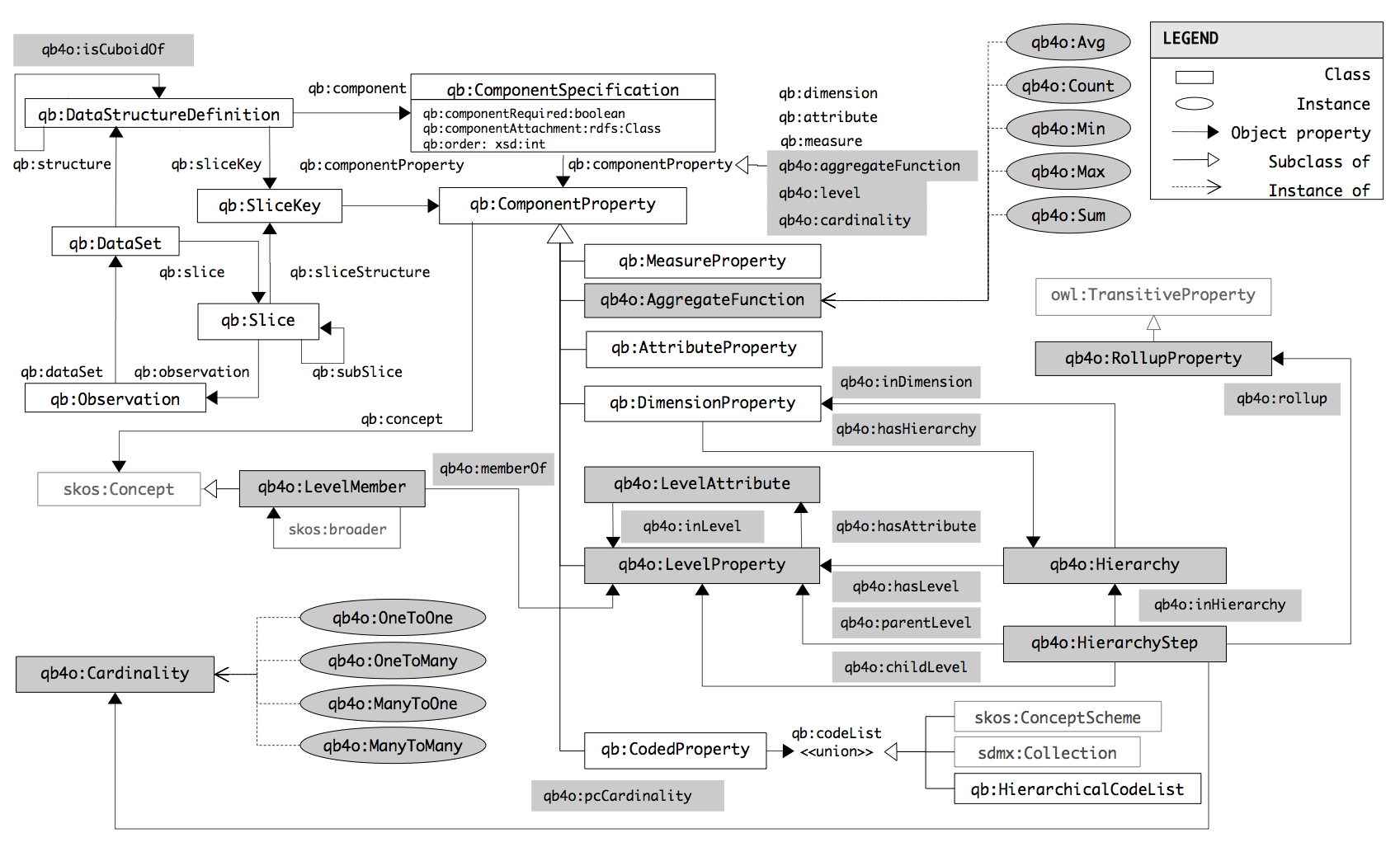
Figure 4: QB4OLAP vocabulary (version 1.3)

The rationale behind QB4OLAP includes:

• QB4OLAP must be able to represent the most common features of the MD model. The features considered are based on the MultiDim model [19].

• QB4OLAP must include all the metadata needed to implement OLAP operations as SPARQL queries. In this way, OLAP users do not need to know SPARQL (which is the case of typical OLAP users), and even wrappers for OLAP tools could be developed to query RDF data sets directly. We comment on this issue at the end of this section.

• QB4OLAP must allow to operate over already published observations which conform to DSDs defined in QB, without the need of rewriting the existing observations, and with the minimum possible effort. Note that in a typical MD model, dimensions are usually orders of magnitude smaller than observations, which are the largest part of the data.

4.2 Implementing data cubes in QB4OLAP

We next sketch how each of the concepts introduced in Section 3.1 can be represented in QB4OLAP. The formal proof is outside the scope of this paper. We assume the reader has basic knowledge of RDF syntax.

Definition 4.1.

(Dimension schema in QB4OLAP) A dimension schema in QB4OLAP is an RDF graph that uses terms defined in the QB and QB4OLAP vocabularies as follows:

• Dimensions are defined as instances of the class
  qb:DimensionProperty.

• Levels are defined as properties, which are instances of the class qb4o:LevelProperty.

• Level attributes are defined as properties, which are instances of the class qb4o:LevelAttribute, and related to levels with the property qb4o:inLevel or its inverse qb4o:hasAttribute.

• Hierarchies are defined as instances of the class
  qb4o:Hierarchy, and related to dimensions with properties qb4o:inDimension and qb4o:hasHierarchy. Levels are connected with the hierarchies they belong using the property qb4o:hasLevel.

• Hierarchies are composed of pairs of levels, which are represented using the class qb4o:HierarchyStep. Pairs are related to hierarchies via the property
  qb4o:inHierarchy. For each pair we distinguish the role of each level using the properties qb4o:childLevel and qb4o:parentLevel.The property qb4o:rollup is used to relate each pair with the property that implements the RUP relation for that step, which is an instance of qb4o:RollupProperty. The cardinality of this relationship (1 to 1, 1 to N, etc.) is stated using the qb4o:pcCardinality property and instances of the qb4o:Cardinality class.

∎

Example 4.1.

(Citizenship dimension schema in QB4OLAP) We show next the representation in QB4OLAP of the schema of the Citizenship dimension of Example 3.1.

⬇

@prefix property: <http://eurostat.linked-statistics.org/property#> .

@prefix schema: <http://www.fing.edu.uy/inco/cubes/schemas/migr_asyapp#> .

@prefix qb4o: <http://purl.org/qb4olap/cubes#> .

schema:citizenshipDim a qb:DimensionProperty ;

rdfs:label "Applicant citizenship dimension"@en;

qb4o:hasHierarchy schema:citizenshipGeoHier, schema:citizenshipGovHier.

# dimension hierarchies

schema:citizenshipGeoHier a qb4o:Hierarchy ;

rdfs:label "Applicant citizenship Geo Hierarchy"@en ;

qb4o:inDimension schema:citizenshipDim;

qb4o:hasLevel property:citizen, schema:continent.

schema:citizenshipGovHier a qb4o:Hierarchy ;

rdfs:label "Applicant citizenship Government Hierarchy"@en ;

qb4o:inDimension schema:citizenshipDim;

qb4o:hasLevel property:citizen, schema:governmentType.

#hierarchy levels and attributes

property:citizen a qb4o:LevelProperty;

rdfs:label "Country of citizenship"@en;

qb4o:hasAttribute schema:countryName.

schema:countryName a qb4o:LevelAttribute;

rdfs:label "Country name"@en ; rdfs:range xsd:string.

schema:continent a qb4o:LevelProperty;

rdfs:label "Continent"@en;

qb4o:hasAttribute schema:continentName.

schema:continentName a qb4o:LevelAttribute;

rdfs:label "Continent name"@en ; rdfs:range xsd:string.

schema:governmentType a qb4o:LevelProperty;

rdfs:label "Government Type"@en;

qb4o:hasAttribute schema:governmentName .

schema:governmentName a qb4o:LevelAttribute;

rdfs:label "Government type name"@en ;rdfs:range xsd:string.

#rollup relationships

schema:inContinent a qb4o:RollupProperty.

schema:hasGovType a qb4o:RollupProperty.

#hierarchy steps

_:ih43 a qb4o:HierarchyStep;

qb4o:inHierarchy schema:citizenshipGeoHier;

qb4o:childLevel property:citizen;

qb4o:parentLevel schema:continent;

qb4o:pcCardinality qb4o:OneToMany;

qb4o:rollup schema:inContinent.

_:ih44 a qb4o:HierarchyStep;

qb4o:inHierarchy schema:citizenshipGovHier;

qb4o:childLevel property:citizen;

qb4o:parentLevel schema:governmentType;

qb4o:pcCardinality qb4o:OneToMany;

qb4o:rollup schema:hasGovType.

Definition 4.2.

(Dimension instance in QB4OLAP) A dimension instance in QB4OLAP is an RDF graph that uses the terms defined in QB and QB4OLAP vocabularies, and also the IRIs defined to represent the dimension schema, as follows: (a) Each level member is represented by an IRI and is related to each level it belongs to, via the qb4o:memberOf property. (b) For each step, the $\mathsf{RUP}$ relation between level members is represented using the property linked to the step in the schema via qb4o:rollup property. ∎

Example 4.2.

(Citizenship dimension instance in QB4OLAP) Below we show part of the triples in the QB4OLAP representation of the instance of the Citizenship dimension in Example 3.2. Note that some triples are enriched with links to external data, like DBpedia.

⬇

@prefix citizen: <http://eurostat.linked-statistics.org/dic/citizen#> .

@prefix citDim: <http://www.fing.edu.uy/inco/cubes/dims/migr_asyapp/citizen#> .

@prefix dbpedia: <http://dbpedia.org/resource/> .

citizen:AD

qb4o:memberOf property:citizen ;

schema:inContinent citizen:EU ;

schema:hasGovType dbpedia:Unitary_state ;

skos:prefLabel "Andorra"@de , "Andorra"@en , "Andorre"@fr .

citizen:ZW

qb4o:inLevel property:citizen ;

schema:inContinent citizen:AF ;

schema:hasGovType dbpedia:Presidential_system;

skos:prefLabel "Simbabwe"@de , "Zimbabwe"@fr , "Zimbabwe"@en .

citizen:EU

qb4o:inLevel schema:continent ;

skos:prefLabel "Europe"@en .

citizen:AF

qb4o:inLevel schema:continent ;

skos:prefLabel "Africa"@en .

dbpedia:Unitary_state

qb4o:inLevel schema:governmentType ;

skos:prefLabel "Unitary state"@en .

…

Definition 4.3.

(Cube schema in QB4OLAP) A cube schema in QB4OLAP is represented as an instance of the qb:DataStructureDefinition class. The dimensions and measures in the cube are represented using the properties qb:measure and qb:dimension. The cardinality between observations and dimensions is represented using the property qb4o:cardinality. Aggregate functions are represented via the qb4o:AggregateFunction, and a property is defined to associate measures with aggregate functions (qb4o:aggregateFunction). This property, allows a given measure to be associated with different aggregate functions in different cubes.

∎

Example 4.3.

(Cube schema in QB4OLAP) We show below the QB4OLAP representation of the Asylum_application cube schema.

⬇

schema:migr_asyappctzmCUBE

rdf:type qb:DataStructureDefinition ;

qb:component [ qb:measure sdmx-measure:obsValue; qb4o:aggregateFunction qb4o:sum ] ;

qb:component [ qb:dimension schema:sexDim ; qb4o:cardinality qb4o:ManyToOne] ;

qb:component [ qb:dimension schema:ageDim ; qb4o:cardinality qb4o:ManyToOne];

qb:component [ qb:dimension schema:timeDim ; qb4o:cardinality qb4o:ManyToOne];

qb:component [ qb:dimension schema:asylappDim ; qb4o:cardinality qb4o:ManyToOne] ;

qb:component [ qb:dimension schema:citizenshipDim ; qb4o:cardinality qb4o:ManyToOne ] ;

qb:component [ qb:dimension schema:destinationDim ; qb4o:cardinality qb4o:ManyToOne] ;

skos:notation "migr_asyappctzmCUBE" .

Definition 4.4.

(Cuboid instance in QB4OLAP) A cuboid instance in QB4OLAP is a set of qb:Observations organized in a qb:DataSet. The set of levels of the cuboid is an instance of the qb:DataStructureDefinition class, and the property qb:structure is used to relate them. To state the fact that a cuboid instance adheres to a specific cube schema we use the property qb4o:isCuboidOf. ∎

Example 4.4.

(Cuboid instance in QB4OLAP) Let us consider the cuboid that corresponds to the schema of Example 4.3, which considers the lowest level for each dimension in the cube (i.e., the bottom of the lattice). Below we show the QB4OLAP representation of the set of levels of the cuboid, the definition of a dataset that represents the cuboid instance, and also a cell in this cuboid (qb:Observation), which corresponds to the last row in Table 2.

⬇

@prefix eurostat: <http://eurostat.linked-statistics.org/data/>

@prefix cell: <<http://eurostat.linked-statistics.org/data/migr_asyappctzm#>

schema:migr_asyappctzmBOTTOM

rdf:type qb:DataStructureDefinition ;

qb4o: isCuboidOf schema:migr_asyappctzmCUBE;

qb:component [ qb:measure sdmx-measure:obsValue; qb4o:aggregateFunction qb4o:sum ] ;

qb:component [ qb4o:level property:age ] ;

qb:component [ qb4o:level sdmx-dimension:refPeriod ] ;

qb:component [ qb4o:level property:sex ] ;

qb:component [ qb4o:level property:geo ] ;

qb:component [ qb4o:level property:citizen] ;

qb:component [ qb4o:level property:asyl_app ] ;

skos:notation "migr_asyappctzmBOTTOM" .

eurostat:migr_asyappctzm

rdf:type qb:DataSet;

qb:structure schema:migr_asyappctzmBOTTOM.

cell:M,CD,F,Y18-34,NASY_APP,BE,2013M03

rdf:type qb:Observation;

qb:dataSet eurostat: migr_asyappctzm;

property:citizen citizen:CD;

property:sex sex:F;

property:age age:Y18-34;

property:asyl_app asyl_app:NASY_APP;

property:geo geo:BE;

measure:obsValue 30;

sdmx-dimension:refPeriod time:201303.

5 Querying Data Cubes

We now present our proposal for querying data cubes on the semantic web. We follow the approach presented in [5], where a clear separation between the conceptual and the logical levels is made. In this way, we formally define a collection of operators, whose semantics is clearly defined using the data model of Section 3.1. This set of operators conforms our query language (QL) at the conceptual level. The user then will write her queries at this level, and they will be translated into a SPARQL query over the QB4OLAP-based RDF representation (at the logical level) using the algorithms presented in Section 5.2 .

5.1 Data Cube Algebra

The operators proposed in the Cube Algebra sketched in [5] can be classified into two groups: (1) Operations that navigate the cube instance to which the input cuboid belongs, which are called instance preserving operations (IPO); and (2) Operations that generate a new cube instance, which are called instance generating operations (IGO). The Roll-up and Drill-down operations belong to the first group, while Slice, Dice and Drill-across belong to the second. We now define each of the operations and provide their semantics.

5.1.1 Instance Preserving Operations (IPO)

IPOs take as input a cuboid in a cube instance, and return another cuboid in the same instance. We consider the following sets: C is the set of all the cuboids in a cube instance, D is the set of dimensions, M is the set of measures, L is the set of dimension levels, and B is the set of boolean expressions over level attributes and measures. For clarity, and to simplify the definitions, we assume that the aggregate function associated to the measures is SUM, so we drop $\mathcal{F}$ from the cube schema definition.

The Roll-up operator is a function Roll-up: $C\times D\times L\rightarrow C$ that summarizes data at a higher level in a dimension hierarchy. It is defined as follows:

Definition 5.1.

(ROLL-UP Operator). Given a cube instance CI with schema $\langle\mathsf{CS},\mathcal{D}_{in},\mathcal{M}_{in}\rangle$, a cuboid $\mathsf{C}_{in}\in\mathsf{CI}$ with its correspondent set of levels $\mathcal{V}_{C_{in}}$, a dimension $\mathsf{D}\in\mathcal{D}_{in}$ with schema $\langle\mathsf{D},\mathcal{L},\rightarrow\rangle$, and two levels $\mathsf{l}_{in},\mathsf{l}_{out}$ in $\mathcal{D}_{in}$ such that: $\mathsf{l}_{in}\in\mathcal{V}_{C_{in}}$ and $\mathsf{l}_{in}\rightarrow^{*}\mathsf{l}_{out}$ in $\langle\mathcal{L},\rightarrow\rangle$, then Roll-up$(\mathsf{C}_{in},\mathcal{D}_{in},\mathsf{l}_{out})$ returns a cuboid $\mathsf{C}_{out}\in\mathsf{CI}$ such that $\mathcal{V}_{C_{out}}=(\mathcal{V}_{C_{in}}-\{\mathsf{l}_{in}\})\cup\{\mathsf{l}_{out}\}$. Notice that $\mathsf{C}_{in}\prec\mathsf{C}_{out}$ in the lattice CI. ∎

The Drill-down operator is a function Drill-down: $C\times D\times L\rightarrow C$ that disaggregates data down to a specific level in a dimension hierarchy.

Definition 5.2.

(DRILL-DOWN Operator). Given a cube instance CI with schema $\langle\mathsf{CS},\mathcal{D}_{in},\mathcal{M}_{in}\rangle$, a cuboid $\mathsf{C}_{in}\in\mathsf{CI}$ with its correspondent set of levels $\mathcal{V}_{C_{in}}$, a dimension $\mathsf{D}\in\mathcal{D}_{in}$ with schema $\langle\mathsf{D},\mathcal{L},\rightarrow\rangle$, and two levels $\mathsf{l}_{in},\mathsf{l}_{out}$ in $\mathcal{D}_{in}$ such that: $\mathsf{l}_{in}\in\mathcal{V}_{C_{in}}$ and $\mathsf{l}_{out}\rightarrow^{*}\mathsf{l}_{in}$ in $\langle\mathcal{L},\rightarrow\rangle$, then Drill-down$(\mathsf{C}_{in},\mathcal{D}_{in},\mathsf{l}_{out})$ returns a cuboid $\mathsf{C}_{out}\in\mathsf{CI}$ such that $\mathcal{V}_{C_{out}}=(\mathcal{V}_{C_{in}}-\{\mathsf{l}_{in}\})\cup\{\mathsf{l}_{out}\}$. Notice that $\mathsf{C}_{out}\prec\mathsf{C}_{in}$ in the lattice CI. ∎

It is straightforward to show, using the lattice of cuboids, that the cuboid produced by a Drill-down on a dimension D is always reachable from the bottom of the lattice, so it can also be obtained performing a Roll-up over the same dimension D from the bottom cuboid. We will use this result in the sequel.

5.1.2 Instance Generating Operations (IGO)

IGOs generate a new cube instance, which may have the same schema than the original one (e.g. in the case of Dice), or may have a different schema (e.g. Slice and Drill-across). In all the cases, these operations take as input a cuboid in a cube instance, and return a cuboid in another instance or cuboid lattice, induced by the application of the operation.

The Dice operator is a function Dice: $C\times B\rightarrow C$ that selects the values in dimension levels and measures that satisfy a boolean condition. It resembles the Selection ($\sigma$) operation in relational algebra.

Definition 5.3.

(DICE Operator). Given a cube instance CI with schema $\langle\mathsf{CS},\mathcal{D}_{in},\mathcal{M}_{in}\rangle$, a cuboid $\mathsf{C}_{in}\in\mathsf{CI}$ with its correspondent set of levels $\mathcal{V}_{C_{in}}$, and a boolean condition $\phi$ over the measures in $\mathcal{M}_{in}$ and/or the attributes of the levels in $\mathcal{V}_{C_{in}}$, Dice$(\mathsf{C}_{in},\phi)$ returns a cuboid $\mathsf{C}_{out}\in C$ as follows:
(a) $c_{i}=(c_{i_{1}},\dots,c_{i_{n}},m_{i_{1}},\dots m_{i_{s}})\in\mathsf{C}_{out}$
if $\exists c_{j}=(c_{j_{1}},\dots,c_{j_{n}},m_{j_{1}},\dots m_{j_{s}})\in\mathsf{C}_{in}$ and $c_{i_{p}}=c_{j_{p}}$ $\forall p,p=1,\dots,n$, $m_{i_{q}}=m_{j_{q}}$ $\forall q,q=1,\dots,s$, and $c_{j}$ satisfies $\phi$;
(b) $\mathcal{V}_{C_{out}}=\mathcal{V}_{C_{in}}$ ∎

The Slice operator is a function Slice: $C\times(D\cup M)\rightarrow C$ that reduces the dimensionality of a cube by removing one of its dimensions or measures. In the case of eliminating a dimension, the Roll-up operation is applied to this dimension in the cuboid before removing it.

Definition 5.4.

(SLICE Operator). Given a cube instance CI with schema $\langle\mathsf{CS},\mathcal{D}_{in},\mathcal{M}_{in}\rangle$, where $\mid\mathcal{D}_{in}\mid>1$ or where $\mid\mathcal{M}_{in}\mid>1$ a cuboid $\mathsf{C}_{in}\in\mathsf{CI}$ with its correspondent set of levels $\mathcal{V}_{C_{in}}$, and a dimension $D\in\mathcal{D}_{in}$ or a measure $M\in\mathcal{M}_{in}$, according to the input parameters:
(1) Slice$(\mathsf{C}_{in},D)$ returns a cuboid $\mathsf{C}_{out}\in C$ as follows:
(a) $c_{i}=(c_{i_{1}},\dots,c_{i_{k-1}},c_{i_{k+1}},m_{i_{1}},\dots m_{i_{s}})\in\mathsf{C}_{out}$
if $\exists c_{j}=(c_{j_{1}},\dots,c_{i_{k-1}},\text{all},c_{i_{k+1}}\dots,c_{j_{n}},m_{j_{1}},\dots m_{j_{s}})\in$Roll-up$(\mathsf{C}_{in},D,All)$ and $c_{i_{p}}=c_{j_{p}}$ $\forall p,p=1,\dots,n$, $p\neq k$, and $m_{i_{q}}=m_{j_{q}}$ $\forall q,q=1,\dots,s$;
(b) $\mathcal{V}_{C_{out}}=\mathcal{V}_{C_{in}}-\{l_{d}\}$, where $l_{d}$ is the level corresponding to dimension $D$ in $\mathsf{C}_{in}$.
(2) Slice$(\mathsf{C}_{in},M)$ returns a cuboid $\mathsf{C}_{out}\in C$ as follows:
(a) $c_{i}=(c_{i_{1}},\dots,c_{i_{n}},m_{i_{1}},\dots,m_{i_{k-1}},m_{i_{k+1}},\dots,m_{i_{s}})\\ \in\mathsf{C}_{out}$  if $\exists c_{j}=(c_{j_{1}},\dots,c_{j_{n}},m_{j_{1}},\dots,m_{j_{k-1}},m_{j_{k}},\\ m_{j_{k+1}},\dots,m_{j_{s}})\in\mathsf{C}_{in}$ and $c_{i_{p}}=c_{j_{p}}$ $\forall p,p=1,\dots,n$, and $m_{i_{q}}=m_{j_{q}}$ $\forall q,q=1,\dots,s$, $q\neq k$;
(b) $\mathcal{V}_{C_{out}}=\mathcal{V}_{C_{in}}$ ∎

The Drill-across operator is a function Drill-across: $C\times C\rightarrow C$ that performs the union of two cuboids that are defined over the same dimensions, and contain the same instance, but differ in the measures. It allows to compare measures from different cuboids and resembles the Join ($\Join$) operation in relational algebra. In this paper we will not address this operator, and limit ourselves to unary operations, that means, operations over single data cubes. Thus, we omit the formal definition of the operation.

5.2 Algebra Operations as SPARQL Queries

Table 1: Auxiliary functions

Function signature	Description
newVarName()	Generates and returns a unique SPARQL variable name.
val(v)	Returns the value stored in variable v
levels(s)	Returns all the levels in a schema s (i.e., all the values of ?l that satisfy s qb:component ?c. ?c qb4o:level ?l)
getLevel(s,d)	Returns the only level l that corresponds to dimension d in the schema s (i.e. the only value of ?l that satisfies s qb:component ?c. ?c qb4o:level ?l. ?h qb4o:hasLevel ?l. ?h qb4o:inDimension ?d)
levelsPath($l_{o}$,$l_{d}$)	Returns a levels path from level $l_{o}$ to $l_{d}$
getRollup($l_{c}$,$l_{p}$)	Resturns the predicate that implements the RUP function from level $l_{c}$ to level $l_{p}$
measures(s)	Returns all the measures in a schema s (all the values of ?m that satisfy s qb:component ?c. ?c qb:measure ?m)
aggFunction(m,s)	Returns the aggregation function of measure m (all the values of ?f that satisfy s qb:component ?c. ?c qb:measure ?m ;qb4o:aggregateFunction ?f).

In this section we show how the operators above can be implemented as SPARQL queries over QB4OLAP-based RDF data cubes. Before that, we would like to discuss on the result form of these queries.

SPARQL queries may return results in different formats. In particular SELECT queries return a table of values, while CONSTRUCT queries return a graph (i.e., a set of triples). Since each operator returns a cuboid in a certain cube instance, and according to Definitions 4.3 and 4.4, cuboids in QB4OLAP are RDF graphs, it is evident that algebra operators should be implemented in SPARQL using CONSTRUCT queries. Despite this, SPARQL 1.1 does not allow to compute aggregations in a CONSTRUCT query, and therefore our approach is to use subqueries. We then produce two queries: (a) an inner SELECT query to compute aggregations, and (b) an outer CONSTRUCT query that generates the graph using the computed results. Notice that the inner query is responsible for the actual computation of values, while the outer query just generates the output as a graph.

We now present the algorithms that generate the SPARQL implementation of each operator. To improve the clarity of the presentation, we use the auxiliary functions defined in Table 1. We also use an abstract representation of a SPARQL query, where for each query: (a) queryType can be SELECT or CONSTRUCT, (b) resultFormat represents the set of variables and expressions included in the SELECT clause or the set of BGPs included in the CONSTRUCT clause, depending on the type of the query, (c) grPatterns represents the set of graph patterns in the WHERE clause, (d) subQueries represents the set of subqueries in the WHERE clause, (e) filter represents a FILTER clause, (f) and groupBy represents the set of variables included in the GROUP BY clause. We assume that each of these parts can be accessed and modified, and we use the dot notation (“.") to access them. We also consider a function $add()$, such that $add(s)$ appends $s$ to a particular part of the query. For example, given a query $q$ such that $q.queryType==$“SELECT” the instruction $q.resultFormat.add(v)$ adds the variable $v$ to the SELECT clause of $q$.

5.2.1 IPO Operations as SPARQL Queries

According to Definition 3.7, a cube instance is the lattice $\{\mathsf{CB},\preceq\}$ where CB is the set of all possible cuboids that adhere to a cube schema, and $\preceq$ is the order between adjacent cuboids in CB. As stated by Definition 3.5 for each pair of adjacent cuboids $\mathsf{Cb}_{1}\preceq\mathsf{Cb}_{2}$, each cell in $\mathsf{Cb}_{2}$ can be computed from the cells in $\mathsf{Cb}_{1}$. Therefore, starting from the bottom cuboid in the lattice, which is the cuboid instance whose cells are members of the bottom levels in each dimension of the schema, all the possible cuboids that form the cube instance can be computed incrementally.

To compute the Roll-up operation over a cuboid $\mathsf{Cb_{in}}$ and a dimension $D$ it suffices to start at $\mathsf{Cb_{in}}$, and navigate the cube lattice visiting adjacent cubes that differ only in the level associated to dimension $D$, until we reach a cuboid $\mathsf{Cb_{out}}$ that has the desired level in dimension $D$ (this path is unique).

Remark 2.

It is not necessary to compute all the cuboids in the path, it suffices to compute the target cuboid. To do so it is necessary to add all the triples needed to traverse the dimension hierarchy up to the target level and aggregate measure values up to this level. ∎

As already mentioned, two SPARQL queries are needed: an inner query $q_{in}$ that traverses the dimension hierarchy and computes aggregate values using GROUP BY, and an outer one, called $q_{out}$ that builds triples based on the values computed in $q_{in}$.

Algorithm 1 builds both queries simultaneously, using the $add$ function. Lines 2 and 3 state the query type for each query. Line 4 states that generated observations belong to the dataset $newDS$. Lines 6 through 12 project the members of each level in the schema into the result of both queries, also adding triples to the WHERE clause of the inner query and adding the variables that represent the level members to the GROUP BY clause also in the inner query. Lines 13 through 19 do the same for measures. In Lines 14 and 18, $f$ represents the SPARQL function corresponding to the aggregate function for each measure, and $f(val(m_{i}))$ is the string that should be included to calculate the aggregated value (e.g $\mbox{{sum}}(?m)$ if $val(m_{i})=?m$). Lines 20 to 33 add the triples needed to navigate the dimension hierarchy. Line 22 retrieves the RDF property that implements the RUP relation for each step in the path. Line 24 adds to the inner query, a triple that associates the level member with the observation (only for the base level $l_{c}$ in dimension D); Line 27 adds a triple that allows us to state to which level the level member belongs, and line 29 retrieves the parent level member of the current level applying the RUP function obtained in Line 22 (this is done for all the levels in the path except for the target level $l_{out}$. When level $l_{out}$ is reached Lines 31 and 32 add the target level to the GROUP BY and SELECT clauses of the inner query, respectively, while Line 33 adds the target level to the outer query result. Finally, Line 34 sets the inner query as a subquery within the WHERE clause of the outer query, which is returned in Line 35. For clarity, we have omitted the clause that generates the expression that binds variable $?newObs$ to a dynamically generated IRI from the values in the observation.

Algorithm 1 Generates a SPARQL query that implements a Roll-up in QB4OLAP

1:$\mathsf{C}_{in}$ is a cuboid instance in QB4OLAP, where $\mathcal{V}_{C_{in}}$ is the set of levels of the cuboid and $d_{r}$ is the dataset that represents the cuboid instance, $l_{out}$ is a level such that $l_{c}\in\mathcal{V}_{C_{in}}$ and $l_{c}\rightarrow^{*}l_{out}$ in the lattice $(\mathcal{L},\rightarrow)$ of a dimension $\mathcal{D}$

2:$q_{out}$ is a SPARQL CONSTRUCT query that represents a cuboid instance $\mathsf{C}_{out}$ = Roll-up$(\mathsf{C}_{in},\mathcal{D},\mathsf{l}_{out})$

3:

4:function CreateRollUpQuery($\mathsf{C}_{in}$, $\mathcal{D}$, $l_{out}$)

5:    $q_{out}$.queryType = ’CONSTRUCT’

6:    $q_{in}$.queryType = ’SELECT’

7:    $q_{out}$.grPatterns.add(?newObs , qb:dataSet , $newDS$)

8:    $l_{c}$ $\leftarrow$ getLevel($C_{in},D$)

9:    for all $l\in L=levels(C_{in})$ do

10:       if $l\neq l_{c}$ then

11:          $l_{i}$ $\leftarrow$ newVar()

12:          $q_{in}$.grPatterns.add(?obs , l, val($l_{i}$))

13:          $q_{in}$.groupBy.add(val($l_{i}$))

14:          $q_{in}$.resultFormat.add(val($l_{i}$))

15:          $q_{out}$.resultFormat.add(?newObs , l, val($l_{i}$))            

16:    for all $m\in M=measures(\mathsf{C}_{in})$ do

17:       f $\leftarrow$ aggFunction(m)

18:       $m_{i}$ $\leftarrow$ newVar()

19:       $ag_{i}$ $\leftarrow$ newVar()

20:       $q_{in}$.grPatterns.add(?obs , m, val($m_{i}$))

21:       $q_{in}$.resultFormat.add(f(val($m_{i}$)) AS $ag_{i}$)

22:       $q_{out}$.resultFormat.add(?newObs , m, val($ag_{i}$))     

23:    for all $(l_{i},l_{j})\in path=levelsPath(l_{c},l_{out})$ do

24:       $lm_{i}$ $\leftarrow$ newVar()

25:       rup $\leftarrow$ getRollup($l_{i},l_{j}$)

26:       if $l_{i}=l_{c}$ then

27:          $q_{in}$.grPatterns.add(?obs , val($l_{i}$), val($lm_{i}$))

28:       else

29:          $plm_{i}$ $\leftarrow$ newVar()

30:          $q_{in}$.grPatterns.add(val($plm_{i}$), qb4o:memberOf, val($l_{i}$))

31:          if $l_{i}\neq l_{out}$ then

32:             $q_{in}$.grPatterns.add(val($lm_{i}$),rup,val($plm_{i}$))

33:          else

34:             $q_{in}$.groupBy.add($plm_{i}$)

35:             $q_{in}$.resulFormat.add($plm_{i}$)

36:             $q_{out}$.resultFormat.add(?newObs , $l_{p}$, val($plm_{i}$))                      

37:    $q_{out}$.subqueries.add($q_{in}$)

38:    return $q_{out}$

Example 5.1.

The SPARQL query generated by Algorithm 1 for RollUp(Asylum_application, Citizenship, Continent) is:

⬇

PREFIX property: <http://eurostat.linked-statistics.org/property#>

PREFIX qb: <http://purl.org/linked-data/cube#>

PREFIX sdmx-dimension: <http://purl.org/linked-data/sdmx/2009/dimension#>

prefix sdmx-measure: <http://purl.org/linked-data/sdmx/2009/measure#>

prefix qb4o: <http://purl.org/qb4olap/cubes#>

prefix schema: <http://www.fing.edu.uy/inco/cubes/schemas/migr_asyapp#>

prefix queries: <http://www.fing.edu.uy/inco/cubes/queries/migr_asyapp#>

CONSTRUCT {

?newObs a qb:Observation ; qb:dataSet queries:ejRollup;

sdmx-dimension:refPeriod ?time ; property:sex ?sex ;

property:geo ?geo; property:age ?age;

property:asyl_app ?apptype; schema:continent ?citContinent ;

sdmx-measure:obsValue ?sumApp }

WHERE {

SELECT ?newObs ?time ?sex ?geo ?age ?apptype ?citContinent (SUM(xsd:integer(?m)) AS ?sumApp)

FROM <http://www.fing.edu.uy/inco/cubes/instances/migr_asyapp_clean>

FROM <http://www.fing.edu.uy/inco/cubes/schemas/migr_asyappctzmQB4O13>

WHERE{

?obs qb:dataSet <http://eurostat.linked-statistics.org/data/migr_asyappctzm> ;

sdmx-dimension:refPeriod ?time ;

property:sex ?sex ; property:geo ?geo ;

property:age ?age; property:asyl_app ?apptype;

sdmx-measure:obsValue ?m ; property:citizen ?citizen .

?citizen qb4o:memberOf property:citizen.

?citizen schema:inContinent ?citContinent. ?citContinent qb4o:memberOf schema:continent.

bind (iri(concat(’http://www.fing.edu.uy/inco/cubes/instances/migr_asyapp’,

md5(concat(str(?time), str(?sex), str(?geo), str(?age), str(?apptype),

str(?citContinent))))) as ?newObs)

}

GROUP BY ?newObs ?time ?sex ?geo ?age ?apptype ?citContinent

}

∎

In Section 5.1 we have discussed that it is possible to transform a Drill-down operation into a Roll-up, therefore there is no need to provide an specific implementation for Drill-down in QB4OLAP.

5.2.2 IGO Operations as SPARQL Queries

IGO operations take as input a cuboid in a cube instance, induce a new cube instance, and return a cuboid in this newly induced lattice of cuboids. In some cases (e.g. Slice) the operations also affect the schema of the cube before producing the cube instance.

The Dice operation takes as input a cuboid in a cube instance, and a boolean expression $\phi$ over measure values and/or attribute values, and returns a cuboid in a new cube instance keeping only the cells from the input cuboid that satisfy $\phi$. The implementation of this operator in SPARQL selects the qb:Observations that satisfy $\phi$. Since measures and attributes are literals, conditions over them can be implemented as FILTER clauses. Also, conditions that only involve equality can be efficiently implemented via graph patterns, restricting the result of the query to observations that are related to a particular level member. Inequalities over level members are represented as FILTER clauses. Algorithm 2 generates the SPARQL implementation of the Dice operator, which is also based in an inner query which performs the filter, and an outer query that produces the results.

Algorithm 2 Generates a SPARQL query that implements a Dice in QB4OLAP

1:$\mathsf{C}_{in}$ is a cuboid instance in QB4OLAP, where with its correspondent set of levels $\mathcal{V}_{C_{in}}$, and a boolean condition $\phi$ over the measures in $\mathcal{M}_{in}$ and/or the attributes of the levels in $\mathcal{V}_{C_{in}}$ $\mathcal{V}_{C_{in}}$ is the set of levels of the cuboid, $\phi$ is a boolean condition over the measures in $\mathcal{M}_{in}$ and/or the attributes of the levels in $\mathcal{V}_{C_{in}}$, and $d_{r}$ is the dataset that represents the cuboid instance

2:$q_{out}$ is a SPARQL CONSTRUCT query that represents a cuboid instance $\mathsf{C}_{out}$ = Dice$(\mathsf{C}_{in},\phi)$

3:

4:function CreateDiceQuery($\mathsf{C}_{in},\phi$)

5:    $q_{out}$.queryType = ’CONSTRUCT’

6:    $q_{in}$.queryType = ’SELECT’

7:    $l_{vars}$ = []

8:    $m_{vars}$ = []

9:    $bgps_{filter}$ = []

10:    $q_{out}$.grPatterns.add(?newObs , qb:dataSet , $newDS$)

11:    for all $l\in L=levels(C_{in})$ do

12:       $l_{i}$ $\leftarrow$ newVar()

13:       $l_{vars}[l]=l_{i}$

14:       $q_{in}$.grPatterns.add(?obs , l, val($l_{i}$))

15:       $q_{in}$.resultFormat.add(val($l_{i}$))

16:       $q_{out}$.resultFormat.add(?newObs , l, val($l_{i}$))     

17:    for all $m\in M=measures(\mathsf{C}_{in})$ do

18:       $m_{i}$ $\leftarrow$ newVar()

19:       $m_{vars}[m]=m_{i}$

20:       $q_{in}$.grPatterns.add(?obs , m, val($m_{i}$))

21:       $q_{in}$.resultFormat.add((val($m_{i}$))

22:       $q_{out}$.resultFormat.add(?newObs , m, val($ag_{i}$))     

23:    $treeCond$ $\leftarrow$ parseCondition($\phi$)

24:    procCondition($treeCond,l_{vars},m_{vars}$, $bgps_{filter}$,$cond_{filter}$)

25:    for all $bgp\in bgps_{filter}$ do

26:       $q_{in}$.grPatterns.add($bgp$)     

27:    $q_{in}$.filter.add($cond_{filter}$)

28:    $q_{out}$.subqueries.add($q_{in}$)

29:    return $q_{out}$

30:$tree$ is a binary tree that represents a boolean condition $\phi$, where internal nodes represent boolean operators (AND,OR,NOT) and leaves represent conditions over level attributes or measure values.$l_{vars}$ is the set of variables that represent level members, $m_{vars}$ is the set of variables that represent measure values

31:$q_{out}$ is a SPARQL CONSTRUCT query that represents a cuboid instance $\mathsf{C}_{out}$ = Dice$(\mathsf{C}_{in},\phi)$

32:

33:function procCondition($tree,l_{vars},m_{vars},bgps,filter$)

34:    if $tree=leaf$ then

35:       if $tree.type="LEVEL"$ then

36:          $v$ $\leftarrow$ findVariable($tree.element,l_{vars}$)

37:          $la$ $\leftarrow$ newVar()

38:          bgps.add($v$ , $tree.level$, $la$)

39:          $filter$ $\leftarrow$ $la$, $tree.oper$, $tree.value$)

40:       else

41:          $v$ $\leftarrow$ findVariable($tree.element,m_{vars}$)

42:          $filter$ $\leftarrow$ $v$, $tree.oper$, $tree.value$)        

43:    else

44:       procCondition($tree.left,l_{vars},m_{vars}$, $bgps_{left}$,$filter_{left}$)

45:       procCondition($tree.right,l_{vars},m_{vars}$, $bgps_{right}$,$filter_{right}$)

46:       bgps.add($bgps_{left}$)

47:       bgps.add($bgps_{right}$)

48:       filter.add($filter_{left}$,$tree.oper$,$filter_{right}$)     

Example 5.2.

(SPARQL query that implements the Dice operation) The operation:
Dice (Asylum_application, ((201303<=month<=201307) $\vee$ (#applications >80) $\wedge$ Destination.country.countryName = Belgium)) is implemented in SPARQL as follows.

⬇

CONSTRUCT { ?o ?p ?v}

WHERE{

SELECT ?o ?p ?v

FROM <http://www.fing.edu.uy/inco/cubes/instances/migr_asyapp_clean>

FROM <http://www.fing.edu.uy/inco/cubes/schemas/migr_asyappctzmQB4O13>

WHERE{

?o a qb:Observation.

?o qb:dataSet <http://eurostat.linked-statistics.org/data/migr_asyappctzm>.

?o sdmx-dimension:refPeriod ?time.

?o sdmx-measure:obsValue ?m.

?o <http://eurostat.linked-statistics.org/property#geo> ?lm1 .

?lm1 <http://www.fing.edu.uy/inco/cubes/schemas/migr_asyapp#countryName> "Belgium"@en .

?time schema:yearMonthNum ?timeMonthNum.

?o ?p ?v.

FILTER (?timeMonthNum >= 201303 && ?timeMonthNum <= 201307&& xsd:integer(?m)>80)

}

}

∎

The Slice operation comes in two flavors. In one case, it takes as input a cuboid instance and a dimension. In the other, it takes a cuboid instance and a measure. In both cases the implementation of this operator in QB4OLAP requires the creation of a new schema, where the input dimension or the measure are removed. In the case where the operation receives a dimension (Slice$(\mathsf{C}_{in},D)$), the new cube instance $\mathsf{C}_{out}$ is computed as (Roll-up$(\mathsf{C}_{in},D,\mathsf{All})$). The SPARQL query generation algorithm is straightforward, and we omit it here.

6 Related Work

There are two main lines of research addressing OLAP analysis of SW data, namely (1) extracting MD data from the SW and loading them into traditional MD data management systems for OLAP analysis; and (2) performing OLAP-like analysis directly over SW data, e.g., over MD data represented in RDF. We next discuss them in some more detail.

Relevant to the first line are the works by Nebot and Llavori [17] and Kämpgen and Harth [14]. The former proposes a semi-automatic method for on-demand extraction of semantic data into a MD database. In this way, data could be analyzed using traditional OLAP techniques. The authors present a methodology for discovering facts in SW data, and populating a MD model with such facts. They assume that data are represented as an OWL ontology. The proposed methodology has four main phases: (1) Design of the MD schema, where the user selects the subject of analysis that corresponds to a concept of the ontology, and then selects potential dimensions. Then, she defines the measures, which are functions over data type properties; (2) Identification and extraction of facts from the instance store according to the MD schema previously designed, producing the base fact table of a DW; (3) Construction of the dimension hierarchies based on the instance values of the fact table and the knowledge available in the domain ontologies (i.e., the inferred taxonomic relationships) and also considering desirable OLAP properties for the hierarchies; (4) User specification of MD queries over the DW. Once queries are executed, a cube is built. Then, typical OLAP operations can be applied over this cube.

Kämpgen and Harth [14] study the extraction of statistical data published using the QB vocabulary into a MD database. The authors propose a mapping between the concepts in QB and a MD data model, and implement these mappings via SPARQL queries. There are four main phases in the proposed methodology: (1) Extraction, where the user defines relevant data sets which are retrieved from the web and stored in a local triple store. Then, SPARQL queries are performed over this triple store to retrieve metadata on the schema, as well as data instances; (2) Creation of a relational representation of the MD data model, using the metadata retrieved in the previous step, and the population of this model with the retrieved data; (3) Creation of a MD model to allow OLAP operations over the underlying relational representation. Such model is expressed using XML for Analysis (XMLA), which allows the serialization of MD models and is implemented by several OLAP clients and servers; (4) Specification of queries over the DW, using OLAP client applications.

The proposals described above are based on traditional MD data management systems, thus they capitalize the existent knowledge in this area and can reuse the vast amount of available tools. However, they require the existence of a local DW to store SW data. This restriction clashes with the autonomous and highly volatile nature of web data sources as changes in the sources may lead not only to updates on data instances but also in the structure of the DW, which would become hard to update and maintain. In addition, these approaches solve only one part of the problem, since they do not consider the possibility of directly querying à la OLAP MD data over the SW.

The second line of research tries to overcome the drawbacks of the first one, exploring data models and tools that allow publishing and performing OLAP-like analysis directly over SW MD data. Terms like self-service BI  [1], Situational BI [16], on-demand BI, or even Collaborative BI, refer to the capability of incorporating situational data into the decision process with little or no intervention of programmers or designers. The web, and in particular the SW, is considered as a large source of data that could enrich decision processes. Abelló et al. [1] present a framework to support self-service BI, based on the notion of fusion cubes, i.e., MD cubes that can be dynamically extended both in their schema and their instances, and in which data and metadata can be associated with quality and provenance annotations.

To support the second approach mentioned above, the RDF Data Cube vocabulary [6] proposes an RDF representation for statistical data according to the SDMX information model. Although similar to traditional MD data models, the SDMX semantics imposes restrictions on what can be represented using QB. Etcheverry and Vaisman [8] proposed QB4OLAP, an extension to QB that allows to represent analytical data according to traditional MD models, also presenting a preliminary implementation of some OLAP operators (Roll-Up, Dice, and Slice), using SPARQL queries over data cubes specified using QB4OLAP.

In [13] the authors present a framework for Exploratory OLAP over Linked Open Data sources, where the MD schema of the data cube is expressed in QB4OLAP and VoID. Based on this MD schema the system is able to query data sources, extract and aggregate data, and build an OLAP cube. The MD information retrieved from external sources is also stored using QB4OLAP.

For an exhaustive study of the possibilities of using SW technologies in OLAP, we refer the reader to the survey by Abelló et al. [2].

7 Conclusion and Future work

In this work, we presented a formal data model for data cubes, that allows the definition of a conceptual query language to manipulate data cubes, and showed that a data cube represented using this model can be published on the semantic web using the QB4OLAP vocabulary. With a focus on querying and publishing data cubes on the semantic web, we defined a conceptual query language for the data model previously described. Finally, we showed how SPARQL queries over QB4OLAP cubes can be automatically produced.

In future work we will concentrate on the composition of operators and the experimental evaluation of this proposal, which, to the best of our knowledge, is the first of its kind.

References

- [1] A. Abelló, J. Darmont, L. Etcheverry, M. Golfarelli, J. Mazón, F. Naumann, T. B. Pedersen, S. Rizzi, J. Trujillo, P. Vassiliadis, and G. Vossen. Fusion cubes: Towards self-service business intelligence. IJDWM, 9(2):66–88, 2013.
- [2] A. Abelló, O. Romero, T. B. Pedersen, R. Berlanga, V. Nebot, M. J. Aramburu, and A. Simitsis. Using semantic web technologies for exploratory olap: A survey. IEEE Transactions on Knowledge and Data Engineering, 27(2):571–588, 2015.
- [3] D. Beckett and T. Berners-Lee. Turtle - Terse RDF Triple Language, 2011.
- [4] D. Brickley, R. Guha, and B. McBride. RDF Vocabulary Description Language 1.0: RDF Schema, 2004.
- [5] C. Ciferri, R. Ciferri, L. Gómez, M. Schneider, A. Vaisman, and E. Zimányi. Cube algebra: A generic user-centric model and query language for OLAP cubes. International Journal of Data Warehousing and Mining, 9(2):39–65, 2013.
- [6] R. Cyganiak and D. Reynolds. The RDF Data Cube Vocabulary (W3C Recommendation), January 2014. http://www.w3.org/TR/vocab-data-cube/.
- [7] L. Etcheverry and A. Vaisman. Enhancing OLAP analysis with web cubes. In Proceedings of ESWC, pages 469–483, Heraklion, Crete, Greece, 2012. Springer.
- [8] L. Etcheverry and A. Vaisman. QB4OLAP: A vocabulary for OLAP cubes on the semantic web. In Proc. of COLD, Boston, USA, 2012. CEUR-WS.org.
- [9] L. I. Gómez, S. A. Gómez, and A. A. Vaisman. A generic data model and query language for spatiotemporal OLAP cube analysis. In Proceedings of EDBT, pages 300–311. ACM, 2012.
- [10] L. I. Gómez, S. A. Gómez, and A. A. Vaisman. A generic data model and query language for spatiotemporal OLAP cube analysis. In Proceedings of EDBT, pages 300–311. ACM, 2012.
- [11] T. Heath and C. Bizer. Linked Data: Evolving the Web into a Global Data Space. Synthesis Lectures on the Semantic Web. Morgan & Claypool Publishers, 2011.
- [12] C. A. Hurtado, A. O. Mendelzon, and A. A. Vaisman. Maintaining Data Cubes under Dimension Updates. In Proceedings of the 15th International Conference on Data Engineering, ICDE ’99, pages 346–355, Washington, DC, USA, 1999. IEEE Computer Society.
- [13] D. Ibragimov, K. Hose, T. Pedersen, and Z. E. Towards exploratory OLAP over linked open data: A case study. In Proceedings of the 7th International Workshop on Business Intelligence for the Real-Time Enterprises, BIRTE 2014. Springer, 2014.
- [14] B. Kämpgen and A. Harth. Transforming statistical linked data for use in OLAP systems. In Proceedings of the 7th International Conference on Semantic Systems, I-Semantics ’11, pages 33–40, New York, NY, USA, 2011. ACM.
- [15] G. Klyne, J. J. Carroll, and B. McBride. Resource Description Framework (RDF): Concepts and Abstract Syntax, 2004.
- [16] A. Löser, F. Hueske, and V. Markl. Situational Business Intelligence. In M. Castellanos, U. Dayal, and V. Markl, editors, Business Intelligence for the Real-Time Enterprise, volume 27 of Lecture Notes in Business Information Processing, pages 1–11. Springer, 2009.
- [17] V. Nebot and R. B. Llavori. Building data warehouses with semantic web data. Decision Support Systems, 52(4):853–868, 2012.
- [18] E. Prud’hommeaux and A. Seaborne. SPARQL 1.1 Query Language for RDF, 2011.
- [19] A. Vaisman and E. Zimányi. Data Warehouse Systems: Design and Implementation. Springer, 2014.
- [20] P. Vassiliadis. Modeling multidimensional databases, cubes and cube operations. In Proceedings of the 10th International Conference on Scientific and Statistical Database Management, SSDBM ’98, pages 53–62, Washington, DC, USA, 1998. IEEE Computer Society.