Large bi-diagonal matrices and random perturbations

Abstract.

This is a first paper by the authors dedicated to the distribution of eigenvalues for random perturbations of large bidiagonal Toeplitz matrices.

Résumé. Ceci est un premier travail par les auteurs sur la distribution des valeurs propres de perturbations aléatoires de grandes matrices bidiagonales de Toeplitz.

1. Introduction and main result

It is well-known that for non-normal operators, as opposed to normal operators, the norm of the resolvent can be very large even far away from the spectrum. Equivalently, the spectrum of such operators can be highly unstable under tiny perturbations. Originating from a renewed interest in numerical analysis with the works of L.N. Trefethen and M. Embree [19, 8], spectral instability of non-self-adjoint operators has become an active subject of interest. It is the source of many interesting effects, as emphasized by the works of E.B. Davies, M. Zworski, J. Sjöstrand and many others (cf. [4, 5, 7, 3, 6]).

It is natural to study the effects of small random perturbations on the spectra of non-normal operators. A recent series of works by M. Hager, W. Bordeaux-Montrieux, J. Sjöstrand and M. Vogel [1, 12, 11, 13, 16, 21, 20] has focused on the case of elliptic (pseudo-)differential operators subject to small random perturbations. It was shown that for a large class of (pseudo-)differential operators one obtains a probabilistic Weyl law for the eigenvalues in the bulk of the spectrum.

Another important example is the case of non-self-adjoint Toeplitz matrices. They can arise for example in models of non-hermitian quantum mechanics, cf [9, 14]. The spectral theory of such operators has been much discussed in the past, cf [22, 2], and from the point of view of spectral instability in [8].

The simplest example of a truncated Toeplitz operator is the Jordan block matrix. M. Hager and E.B. Davies [6] considered the case of large Jordan block matrices subject to small Gaussian random perturbations and showed that with a sufficiently small coupling constant most eigenvalues can be found near a circle, with probability close to $1$, as the dimension of the matrix $N$ gets large. Furthermore, they give a probabilistic upper bound of order $\log N$ for the number of eigenvalues in the interior of a circle.

A recent result by A. Guionnet, P. Matched Wood and O. Zeitouni [10] implies that when the coupling constant is bounded from above and from below by (different) sufficiently negative powers of $N$, then the normalized counting measure of eigenvalues of the randomly perturbed Jordan block converges weakly in probability to the uniform measure on $S^{1}$ as the dimension of the matrix gets large.

In [15], J. Sjöstrand obtained a probabilistic circular Weyl law for most of the eigenvalues of large Jordan block matrices subject to small random perturbations, and in [17], we obtained a precise asymptotic formula for the average density of the residual eigenvalues in the interior of a circle, where the result of Davies and Hager yielded a logarithmic upper bound on the number of eigenvalues. The leading term is given by the hyperbolic volume form on the unit disk, independent of the dimension $N$.

The goal of the present work is to study the spectrum of random perturbations of the following bidiagonal $N\times N$ Toeplitz matrix:

• (1.1) $$P=P_{\mathrm{I}}=\begin{pmatrix}0&a&0&..&..&0\\ b&0&a&..&..&0\\ 0&b&0&..&..&0\\ ..&..&..&..&..&..\\ 0&..&..&..&0&a\\ 0&0&..&..&b&0\end{pmatrix}$$

Originally we also wanted to include

• (1.2) $$P=P_{\mathrm{II}}=\begin{pmatrix}0&a&b&0&..&..&0\\ 0&0&a&b&..&..&0\\ 0&0&0&a&..&..&0\\ ..&..&..&..&..&..&..\\ ..&..&..&..&..&a&b\\ ..&..&..&..&..&0&a\\ ..&..&..&..&..&0&0\end{pmatrix},$$

  but we decided to postpone much of the study in this case.

Here $a,\,b\in{\bf C}\setminus\{0\}$ and $N\gg 1$. Identifying ${\bf C}^{N}$ with $\ell^{2}([1,N])$, $[1,N]=\{1,2,..,N\}$ and also with $\ell^{2}_{[1,N]}({\bf Z})$ (the space of all $u\in\ell^{2}({\bf Z})$ with support in $[1,N]$), we have:

(1.3) $$P_{\mathrm{I}}=1_{[1,N]}(a\tau_{-1}+b\tau_{1})=1_{[1,N]}(a\mathrm{e}^{iD_{x}}+b\mathrm{e}^{-iD_{x}}),$$

(1.4) $$P_{\mathrm{II}}=1_{[1,N]}(a\tau_{-1}+b\tau_{-2})=1_{[1,N]}(a\mathrm{e}^{iD_{x}}+b\mathrm{e}^{2iD_{x}}),$$

where $\tau_{k}u(j)=u(j-k)$ denotes translation by $k$.

The symbols of these operators are by definition,

(1.5) $$P_{\mathrm{I}}(\xi)=a\mathrm{e}^{i\xi}+b\mathrm{e}^{-i\xi},\ P_{\mathrm{II}}(\xi)=a\mathrm{e}^{i\xi}+b\mathrm{e}^{2i\xi}.$$

In this work, we consider the following random perturbation of $P_{0}=P_{\mathrm{I}}$

(1.6) $$P_{\delta}:=P_{0}+\delta Q_{\omega},\quad Q_{\omega}=(q_{j,k}(\omega))_{1\leq j,k\leq N},$$

where $0\leq\delta\ll 1$ and $q_{j,k}(\omega)$ are independent and identically distributed complex Gaussian random variables, following complex Gaussian law $\mathcal{N}_{\mathbf{C}}(0,1)$.
The following result shows that, with probability close to $1$, most eigenvalues are in a small neighbourhood of the ellipse $E_{1}=P_{\mathrm{I}}(S^{1})$ with focal points $\pm 2\sqrt{ab}$ and major semi-axis of length $|a|+|b|$: let $\gamma$ be a segment of $E_{1}$ and $r>0$, put

(1.7) $$\Gamma(r,\gamma)=\{z\in\mathbf{C};~{}\mathrm{dist}(z,E_{1})=\mathrm{dist}(z,\gamma)<r\}.$$

Theorem 1.1.

Let $P=P_{\mathrm{I}}$ be the bidiagonal matrix in (1.1) where $a,b\in{\bf C}$ satisfy $0<|b|<|a|$. Let $P_{\delta}$ be as in (1.6). Choose $\delta\asymp N^{-\kappa}$, $\kappa>5/2$ and consider the limit of large $N$. Let $\gamma$ be a segment of the ellipse $E_{1}=P_{\mathrm{I}}(S^{1})$ and let $\Gamma=\Gamma(r,\gamma)$ be as in (1.7) with $(\ln N)/N\ll r\ll 1$. Let $\delta_{0}$ be small and fixed.

Then with probability

(1.8) $$\geq 1-\mathcal{O}(1)\left(\frac{1}{r}+\ln N\right)N^{2\kappa}\mathrm{e}^{-2N^{\delta_{0}}},$$

we have

(1.9) $$\left|\#(\sigma(P_{\delta})\cap\Gamma)-\frac{1}{2\pi}\mathrm{vol}_{]0,N]\times S^{1}}P_{\mathrm{I}}^{-1}(\Gamma)\right|\leq{\mathcal{O}}(1)N^{\delta_{0}}(\frac{1}{r}+\ln N).$$

If we choose $\gamma=E^{1}$ and view $P_{\mathrm{I}}$ as a function on $]0,N]\times S^{1}$, then, since $P_{\mathrm{I}}^{-1}(\Gamma)=P_{\mathrm{I}}^{-1}(E_{1})=]0,N]\times S^{1}$, we have

$$\frac{1}{2\pi}\mathrm{vol}_{]0,N]\times S^{1}}P_{\mathrm{I}}^{-1}(\Gamma)=N$$

which is equal to the total number of eigenvalues of $P_{\delta}$, so the number of eigenvalues outside of $\Gamma$ is bounded be the right hand side of (1.9). With $r>0$ fixed but arbitrarily small we get

Corollary 1.2.

Under the general assumptions in Theorem 1.1, let $\Gamma$ be any fixed neighborhood of $E_{1}$. Then with probability as in (1.8), we have

(1.10) $$\left|\#\left(\sigma(P_{\delta})\cap({\bf C}\setminus\Gamma)\right)\right|\leq{\mathcal{O}}(1)N^{\delta_{0}}\ln N.$$

Figure 1 illustrates the result of Theorem 1.1 by showing the eigenvalues of the $N\times N$-matrix in (1.1), with $N=500$, $a=1+i$ and $b=0.5$, perturbed with a complex Gaussian random matrix and coupling constant $\delta=10^{-5}$. The line indicates the image of the unit circle $S^{1}$ under the symbol of the matrix (1.1). We can see that most eigenvalues are close to an ellipse with only very few in the interior. This phenomenon has been observed numerically in [8] (we refer in particular to Figures 3.2 and 3.3 in [8]). For more numerical simulations for more general Toeplitz matrices, we refer the reader to [8, Section 7].

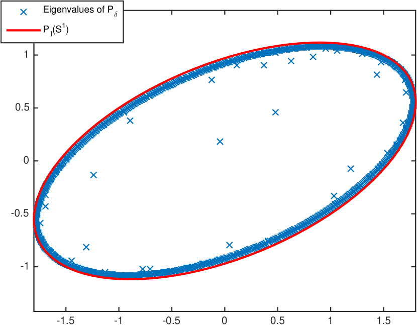
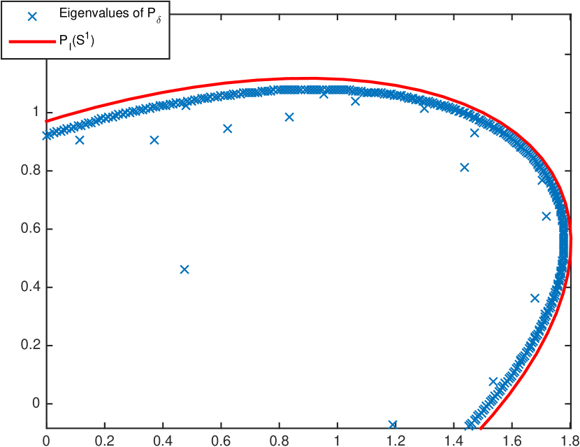
Figure 1. The spectrum of $P_{I}$ with $N=500$, $a=1+i$ and $b=0.5$ perturbed with a complex Gaussian random Matrix with coupling constant $\delta=10^{-5}$. The red line is the image of the unit circle $S^{1}$ under the symbol $P_{\mathrm{I}}$.

Acknowledgements. J. Sjöstrand was supported by the project NOSEVOL ANR 2011 BS 01019 01. M. Vogel was supported by the projects GeRaSic ANR-13-BS01-0007-01 and NOSEVOL ANR 2011 BS 01019 01.

2. The range of the symbol

Write

(2.1) $$a=|a|e^{i\alpha},\ b=|b|e^{i\beta},\ \ \alpha,\beta\in{\bf R}.$$

2.1. Case I

We have $P(\xi)=|a|e^{i(\alpha+\xi)}+|b|e^{i(\beta-\xi)}$ and the largest value of $|P(\xi)|$ (for $\xi$ real) is attained when the two terms in the expression for $P(\xi)$ point in the same direction. This happens precisely when

$$\xi=\frac{\beta-\alpha}{2}+\pi k,\ k\in{\bf Z}.$$

Write $\xi=\frac{\beta-\alpha}{2}+\eta$. Then

(2.2) $$\begin{split}P(\xi)&=e^{i\frac{\alpha+\beta}{2}}(|a|e^{i\eta}+|b|e^{-i\eta})\\ &=e^{i\frac{\alpha+\beta}{2}}\left((|a|+|b|)\cos\eta+i(|a|-|b|)\sin\eta\right).\end{split}$$

Assume, to fix the ideas, that $|b|\leq|a|$. Then $P({\bf R})$ is equal to the ellipse, $E_{1}$, centred at 0 with major semi-axis of length $(|a|+|b|)$ pointing in the direction $e^{i(\alpha+\beta)/2}$ and minor semi-axis of length $|a|-|b|$. The focal points of $E_{1}$ are

(2.3) $$\pm 2\sqrt{ab}=\pm e^{i\frac{\alpha+\beta}{2}}2\sqrt{|a||b|}.$$

The left hand side of Figure 2 illustrates the range of the symbol in case I by presenting $P(S^{1})$ with $b=0.5$ and $a=1+i$, $a=0.5+0.5i$.

2.2. Case II

Write

$$P=|a|e^{i(\alpha+\xi)}+|b|e^{i(\beta+2\xi)}.$$

By the same reasoning as in Case I, the largest value, $|a|+|b|$, of $|P(\xi)|$ is attained when

$$\xi=\xi_{\mathrm{max}}:=\alpha-\beta+2\pi k,\ k\in{\bf Z}.$$

The smallest value $||a|-|b||$ of $|P(\xi)|$ is attained when

$$\xi=\xi_{\mathrm{min}}:=\alpha-\beta+\pi+2\pi k.$$

We have

(2.4) $$P(\xi_{\mathrm{max}})=e^{i(2\alpha-\beta)}(|a|+|b|),\ P(\xi_{\mathrm{min}})=-e^{i(2\alpha-\beta)}(|a|-|b|).$$

Write $\xi=\alpha-\beta+\eta$, so that

(2.5) $$P(\xi)=e^{i(2\alpha-\beta)}f(e^{i\eta}),\ \ f(\zeta)=|a|\zeta+|b|\zeta^{2}.$$

The study of $P({\bf R})$ is equivalent to that of $f(S^{1})$. Assume for notational reasons that $a,b>0$, so that

$$f=f_{a,b}(\zeta)=a\zeta+b\zeta^{2}.$$

This function has the unique critical point $\zeta=\zeta_{c}(a,b)$, given by $a+2b\zeta_{c}=0$,

(2.6) $$\zeta_{c}=-\frac{a}{2b}$$

and

(2.7) $$f(\zeta_{c})=-\frac{a^{2}}{4b}.$$

Since $f$ is quadratic, we have

(2.8) $$f(\zeta)=f(\zeta_{c})+b(\zeta-\zeta_{c})^{2}=-\frac{a^{2}}{4b}+b\left(\zeta+\frac{a}{2b}\right)^{2}.$$

Notice that

• $b<a/2$ $\Longrightarrow$ $\zeta_{c}\not\in\overline{D(0,1)}$,

• $b=a/2$ $\Longrightarrow$ $\zeta_{c}\in S^{1}$,

• $b>a/2$ $\Longrightarrow$ $\zeta_{c}\in D(0,1)$.

In the first case there is no pair of distinct points on $S^{1}$ which are symmetric to each other with respect to $\zeta_{c}$ so $f(S^{1})$ is a simple closed curve in ${\bf C}$.

In the second case $f:S^{1}\to{\bf C}$ is still injective but has a critical point at $\zeta_{c}$. The image of $S^{1}$ is still a simple closed curve, but with a cusp at $f(\zeta_{c})$.

In the third case, the critical point $\zeta_{c}$ is situated on the segment $]-1,0[$. There is one pair of points on $S^{1}$ that are symmetric to each other with respect to $\zeta_{c}$, namely $\alpha_{c}$ and $\overline{\alpha_{c}}$, where $\alpha_{c}=\zeta_{c}+i\sqrt{1-\zeta_{c}^{2}}$. Thus $f(\alpha_{c})=f(\overline{\alpha_{c}})\in]-\infty,f(\zeta_{c})[$ is the only point in $f(S^{1})$ whose inverse image consists of more than one point. $f(S^{1})$ is a closed curve with $f(\alpha_{c})=f(\overline{\alpha_{c}})$ as its unique point of self intersection. We can write

(2.9) $$f(S^{1})=\{f(\alpha_{c})\}\cup\gamma_{\mathrm{int}}\cup\gamma_{\mathrm{ext}},$$

where $\gamma_{\mathrm{int}}=f(S^{1}\cap\{\zeta;\Re\zeta<\Re\zeta_{c}\})$, $\gamma_{\mathrm{ext}}=f(S^{1}\cap\{\zeta;\Re\zeta>\Re\zeta_{c}\})$ are smooth curves, which become simple closed after adding $f(\zeta_{c})$ and $\gamma_{\mathrm{int}}$ is situated in the interior of the region enclosed by the closure of $\gamma_{\mathrm{ext}}$.

The right hand side of Figure 2 illustrates the range of the symbol in case II by presenting $P(S^{1})$ with $b=0.5$ and $a=i$, $a=0.4i$.

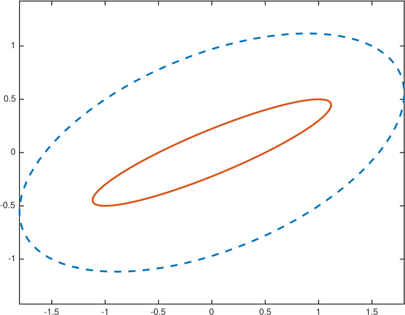
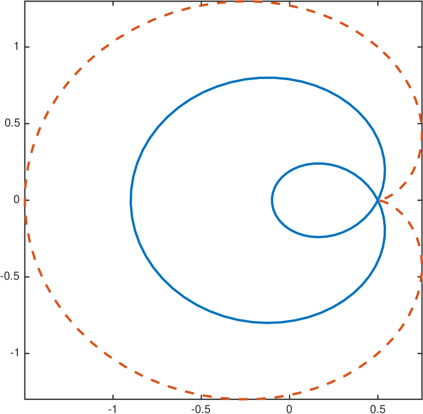
Figure 2. The left hand side shows the image of $S^{1}$ under the principal symbol of case I (for the dashed ellipse we chose $b=0.5$, $a=1+i$ and for the other ellipse $b=0.5$, $a=0.5+0.5i$). The right hand side is similar but for the principal symbol of case II (for the dashed line we chose $b=0.5$, $a=i$ and for the continuous line $b=0.5$, $a=0.4i$).

3. Numerical range

In case I, we can write

(3.1) $$\begin{split}&P=1_{[1,N]}e^{i\frac{\alpha+\beta}{2}}\times\\ &\left((|a|+|b|)\cos\left(hD_{x}-\frac{\beta-\alpha}{2}\right)+i(|a|-|b|)\sin\left(hD_{x}-\frac{\beta-\alpha}{2}\right)\right).\end{split}$$

$\cos(hD-(\beta-\alpha)/2)$ and $\sin(hD-(\beta-\alpha)/2)$ are bounded self-adjoint operators on $\ell^{2}({\bf Z})$, of norm $\leq 1$. If $u\in\ell^{2}([1,N])$ the quantities

$$J(u)=(1_{[1,N]}\cos(hD-(\beta-\alpha)/2)u|u)=(\cos(hD-(\beta-\alpha)/2)u|u)$$

and

$$K(u)=(1_{[1,N]}\sin(hD-(\beta-\alpha)/2)u|u)=(\sin(hD-(\beta-\alpha)/2)u|u)$$

are real and belong to $[-\|u\|^{2},\|u\|^{2}]$, and we observe that

(3.2) $$(Pu|u)=e^{i\frac{\alpha+\beta}{2}}((|a|+|b|)J(u)+i(|a|-|b|)K(u)).$$

By Cauchy-Schwartz,

$$J(u)^{2}\leq\|\cos(hD-(\beta-\alpha)/2)u\|^{2}\|u\|^{2}=\left(\cos^{2}(hD-(\beta-\alpha)/2)u|u\right)\|u\|^{2},$$

and similarly,

$$K(u)^{2}\leq\left(\sin^{2}(hD-(\beta-\alpha)/2)u|u\right)\|u\|^{2}.$$

Summing the two estimates and using that $\cos^{2}+\sin^{2}=1$, it follows that

$$\sqrt{J(u)^{2}+K(u)^{2}}\leq\|u\|^{2}.$$

If we take $u$ normalised, we deduce from this and (3.2) that

Proposition 3.1.

In case I, the numerical range of $P=P_{\mathrm{I}}$ is contained in the convex hull of the ellipse $E_{1}$ described after (2.2).

In case II, we have the trivial inclusion,

$$\mathrm{Num\,Range}(P_{\mathrm{II}})\subset D(0,|a|+|b|).$$

Using semi-classical analysis and especially the sharp Gårding inequality, it seems clear that the numerical range is contained in a $1/N$-neighborhood of the convex hull of $P(S^{1})$.

4. Spectrum of the unperturbed operator

4.1. Case I

The spectrum of $P_{\mathrm{I}}$ as a set coincides with the set of eigenvalues. Consider an eigenvalue $z\in{\bf C}$ and a corresponding eigenvector $0\neq u\in\ell^{2}([1,N])$. Extending $u$ to $[0,N+1]$ by putting $u(0)=0$, $u(N+1)=0$, we have

(4.1) $$au(k+1)-zu(k)+bu(k-1)=0,\ k=1,...,N.$$

We can extend $u$ further to all of ${\bf Z}$ and get a function $\widetilde{u}:{\bf Z}\to{\bf C}$ such that

(4.2) $$\widetilde{u}(k)=u(k)\hbox{ on }[1,N],\ \widetilde{u}(0)=\widetilde{u}(N+1)=0$$

and such that

(4.3) $$a\widetilde{u}(k+1)-z\widetilde{u}(k)+b\widetilde{u}(k-1)=0,\ k\in{\bf Z}.$$

The space of solutions to (4.3) is of dimension 2 and if the equation

(4.4) $$a\zeta+b/\zeta-z=0$$

has two distinct solutions $\zeta_{+}$ and $\zeta_{-}$, then it is generated by the functions $\widetilde{u}_{\pm}$, given by

(4.5) $$\widetilde{u}_{\pm}(k)=\zeta_{\pm}^{k},\ k\in{\bf Z}.$$

When the equation has a double solution, which happens precisely when

(4.6) $$a\zeta=\frac{b}{\zeta}=\frac{z}{2},$$

i.e. when $z$ is one of the focal points of $E_{1}$, the same space is generated by

(4.7) $$\widetilde{u}_{0}(k)=\zeta^{k},\widetilde{u}_{1}(k)=k\zeta^{k}.$$

In the case when the characteristic equation has two distinct solutions, we can write

$$\widetilde{u}(k)=c_{+}\zeta_{+}^{k}+c_{-}\zeta_{-}^{k},$$

and apply the boundary conditions in (4.2), to get

$$c_{+}+c_{-}=0,\ \ c_{+}\zeta_{+}^{N+1}+c_{-}\zeta_{-}^{N+1}=0,$$

to get

(4.8) $$c_{-}=-c_{+},\ \ \zeta_{+}^{N+1}=\zeta_{-}^{N+1}.$$

This gives the $N$ possibilities,

(4.9) $$\frac{\zeta_{+}}{\zeta_{-}}=e^{2\pi i\nu/(N+1)},\ \nu=1,2,...,N.$$

(The case $\nu=0$ is excluded since we are in the case of distinct solutions of the characteristic equation.) The relation between the two solutions of (4.4) is given by

(4.10) $$a\zeta_{+}=b/\zeta_{-},$$

and insertion of this in (4.9) gives,

$$\frac{a}{b}\zeta_{+}^{2}=e^{2\pi i\nu/(N+1)}.$$

Fixing a branch of $\sqrt{b/a}$, we get

(4.11) $$\zeta_{\pm}(\nu)=\sqrt{b/a}e^{\pm\pi i\nu/(N+1)},\nu=1,...,N.$$

The corresponding eigenvalues are then

(4.12) $$z=z(\nu)=a\zeta_{+}(\nu)+b/\zeta_{+}(\nu)=2\sqrt{ab}\cos\left(\frac{\pi\nu}{N+1}\right).$$

These values are distinct so we conclude that the spectrum of $P_{\mathrm{I}}$ consists of $N$ simple eigenvalues.

Recall the representation (2.1). We can choose the branch of the square root so that

$$\sqrt{ab}=\sqrt{|a||b|}e^{i(\alpha+\beta)/2}.$$

We conclude that the eigenvalues

(4.13) $$z(\nu)=2\sqrt{|a||b|}e^{i(\alpha+\beta)/2}\cos\left(\frac{\pi\nu}{N+1}\right)$$

are situated on the major axis of the ellipse $E_{1}$, between the two focal points (2.3).

Remark 4.1.

Let $W=\mathrm{diag\,}(w^{k})_{0\leq k\leq N-1}$ be the diagonal matrix with elements $w^{k}$, $1\leq k\leq N$, where $0\neq w\in{\bf C}$. Then $P$ has the same spectrum as

$$\widetilde{P}=WPW^{-1}=\begin{pmatrix}0&a/w&0&..&..&0\\ bw&0&a/w&..&..&0\\ 0&bw&0&a/w&..&0\\ ..&..&..&..&..&..\\ ..&..&..&bw&0&a/w\\ ..&..&..&..&bw&0\end{pmatrix},$$

and choosing $w=(a/b)^{1/2}$ gives

$$\widetilde{P}=(ab)^{1/2}\begin{pmatrix}0&1&0&..&..&..&0\\ 1&0&1&..&..&..&0\\ 0&1&0&1&..&..&0\\ ..&..&..&..&..&..&..\\ ..&..&..&..&..&..&..\\ ..&..&..&..&1&0&1\\ ..&..&..&..&..&1&0\end{pmatrix},$$

The last matrix is self-adjoint and this explains why the eigenvalues of $P$ are situated on a segment.

4.2. Case II

$P=P_{\mathrm{II}}$ is nilpotent, so

(4.14) $$\sigma(P)=\{0\}.$$

5. Size of $|\zeta|$

For the understanding of our operators, it will be important do determine, depending on $z$, the number of exponential solutions $\widetilde{u}(k)=\zeta^{k}$ that grow near $k=+\infty$ and near $k=-\infty$ respectively. Here $\zeta$ is a solution of the characteristic equation (4.4) in case I and of the characteristic equation

(5.1) $$a\zeta+b\zeta^{2}=z$$

in case II.

5.1. Case I

We recall that we have assumed for simplicity that $|a|\geq|b|$. The case $|a|=|b|$ will be obtained as a limiting case of the one when $|a|>|b|$, that we consider now. Let

$$f_{a,b}(\zeta)=a\zeta+b/\zeta$$

and observe that when $r>0$

$$f_{a,b}(\partial D(0,r))=f_{ar,b/r}(\partial D(0,1))$$

which gives a family of confocal ellipses $E_{r}$. The length of the major semi-axis of $E_{r}$ is equal to $|a|r+|b|/r=:g(r)$. $E_{r_{1}}$ is contained in the bounded domain which has $E_{r_{2}}$ as its boundary, precisely when $g(r_{1})\leq g(r_{2})$. The function $g$ has a unique minimum at $r=r_{\mathrm{min}}=(|b|/|a|)^{1/2}$. $g$ is strictly decreasing on $]0,r_{\mathrm{min}}]$ and strictly increasing on $[r_{\mathrm{min}},+\infty[$. It tends to $+\infty$ when $r\to 0$ and when $r\to+\infty$. We have $g_{\mathrm{min}}=g(r_{\mathrm{min}})=2(|a||b|)^{1/2}$ so $E_{r_{\mathrm{min}}}$ is just the segment between the two focal points, common to all the $E_{r}$. For $r\neq r_{\mathrm{min}}$, the map $\partial D(0,r)\to E_{r}$ is a diffeomorphism. Let $r_{1}$ be the unique value in $]0,1[$ for which $g(r_{1})=|a|+|b|=g(1)$. We get the following result:

Proposition 5.1.

Let $|b|<|a|$.

• When $z$ is strictly inside the ellipse $E_{1}$ described after (2.2), then both solutions of $f_{a,b}(\zeta)=z$ belong to $D(0,1)$.

• When $z$ is on the ellipse, one solution is on $S^{1}$ and the other belongs to $D(0,1)$.

• When $z$ is in the exterior region to the ellipse, one solution fulfills $|\zeta|>1$ and the other satisfies $|\zeta|<1$.

Proof.

When $z$ is strictly inside $E_{1}$ it belongs to $E_{\rho_{-}}=E_{\rho_{+}},$ $E_{\rho_{\pm}}=f(\partial D(0,\rho_{\pm}))$, for $r_{1}<\rho_{-}\leq\rho_{+}<1$ and $\zeta_{\pm}\in\partial D(0,\rho_{\pm})$. The other two cases are treated similarly. ∎

In the case $|a|=|b|$, $E_{1}$ is just the segment between the two focal points. In this case $r_{\mathrm{min}}=1$ and we get:

Proposition 5.2.

Assume that $|a|=|b|$.

• If $z\in E_{1}$ then both solutions of $f_{a,b}(\zeta)=z$ belong to $S^{1}$.

• If $z$ is outside $E_{1}$, one solution is in $D(0,1)$ and the other is in the complement of $\overline{D(0,1)}$.

Remark 5.3.

Recall that $E_{\rho}$ is the ellipse with focal points $\pm c=\pm 2\sqrt{ab}$ and length of major semi-axis equal to $g(\rho):=a\rho+b/\rho$. Equivalently,

$$E_{\rho}=\{z\in{\bf C};\,|z-c|+|z+c|=2g(\rho)\}.$$

The solutions $\zeta=\zeta_{\pm}$ of $f_{a,b}(\zeta)=z$ belong to $\partial D(0,\rho_{\pm})$, where $\rho_{\pm}$ are the solutions to $2g(\rho_{\pm})=|z-c|+|z+c|$, situated on each side of $r_{\mathrm{min}}=\sqrt{b/a}$. Also, $g_{\mathrm{min}}=g(r_{\mathrm{min}})=|c|$.

Assume that $z$ is restricted to a compact subset $K$ of ${\bf C}$. Then $\rho_{\pm}\in[1/C,C]$ for some $C=C(K)>1$. For $\rho\in[1/C,C]$, we have

$$g(\rho)-|c|\asymp|\rho-r_{\mathrm{min}}|^{2}.$$

Consequently,

$$|\rho_{\pm}-r_{\mathrm{min}}|\asymp(g(\rho_{\pm})-|c|)^{\frac{1}{2}}=(|z-c|+|z+c|-2|c|)^{\frac{1}{2}}.$$

Since $\rho_{\pm}$ are situated on opposite sides of $r_{\mathrm{min}}$; we get

(5.2) $$|\zeta_{+}-\zeta_{-}|\geq|\rho_{+}-\rho_{-}|\asymp(|z-c|+|z+c|-2|c|)^{\frac{1}{2}}$$

5.2. Case II

Can be removed from this paper We write the equation (5.1) as

(5.3) $$f(\zeta)=z,\hbox{ where }f(\zeta):=a\zeta+b\zeta^{2}=b(\zeta-\zeta_{c})^{2}+c=z,$$

$\zeta_{c}$ is the critical point, given by $\zeta_{c}=-a/(2b)$ and

$$c=f(\zeta_{c})=-a^{2}/(4b).$$

For any given $z$, the two solutions are symmetric around $\zeta_{c}$, and depending on in which case we are according to the conclusion after (2.8), we just have to see if both, one or none of the symmetric solutions belong to $D(0,1)$.

When $|b|<|a|/2$, we have $\zeta_{c}\not\in\overline{D(0,1)}$, $f(S^{1})$ is a simple smooth closed curve $\gamma$ and if we let $\Gamma$ be the bounded open set with $\partial\Gamma=\gamma$, we conclude:

Proposition 5.4.

• If $z\in\Gamma$, then one of the solutions belongs to $D(0,1)$ and the other one is in ${\bf C}\setminus\overline{D(0,1)}$.

• If $z\in\gamma$, then one of the solutions belongs to $S^{1}$ and the other is in ${\bf C}\setminus\overline{D(0,1)}$.

• If $z\in{\bf C}\setminus\overline{\Gamma}$, then both solutions are in $z\in{\bf C}\setminus\overline{D(0,1)}$.

When $|b|=|a|/2$, we have:

Proposition 5.5.

For $z\neq f(\zeta_{c})$ (i.e. for $z$ away from the cusp of the simple closed curve $f(S^{1})$) we have the same conclusion as in Proposition 5.4. When $z=f(\zeta_{c})$ (i.e. at the cusp), $\zeta=\zeta_{c}\in S^{1}$ is a double solution of $z=f(\zeta)$ (and there is no other).

When $|b|>|a|/2$, we have $\zeta_{c}\in D(0,1)$ and $\zeta_{c}\neq 0$. Draw the line through $\zeta_{c}$ which is perpendicular to the radius of $D(0,1)$ that passes through that point and let $\alpha_{c}$ and $\alpha^{\prime}_{c}$ be the two points of intersection with $S^{1}$. We have seen in Section 2 that $f(\alpha_{c})=f(\alpha^{\prime}_{c})$ and that the short circle arcs and the long circle arcs connecting these two points are mapped by $f$ onto two simple closed curves $\gamma_{\mathrm{int}}$ and $\gamma_{\mathrm{ext}}$, both containing the point $f(\alpha_{c})=f(\alpha^{\prime}_{c})$ and such that if we let $\Gamma_{\mathrm{int}}$, $\Gamma_{\mathrm{ext}}$ denote the open bounded sets bounded by $\gamma_{\mathrm{int}}$, $\gamma_{\mathrm{ext}}$ respectively, then away from $f(\alpha_{c})$, $\gamma_{\mathrm{int}}$ is contained in $\Gamma_{\mathrm{ext}}$. Also $\Gamma_{\mathrm{int}}\subset\Gamma_{\mathrm{ext}}$.

It is geometrically clear that the set of points $\zeta$ in $\overline{D(0,1)}$ for which the symmetric point with respect to $\zeta_{c}$, namely $\zeta^{\prime}=\zeta_{c}-(\zeta-\zeta_{c})$, also belongs to $\overline{D(0,1)}$, is obtained by taking the short circular segment from $\alpha_{c}$ to $\alpha^{\prime}_{c}$, then the convex hull of that set and finally adding all the symmetric points with respect to $\zeta_{c}$. This is a lens shaped region $L$ inside $\overline{D(0,1)}$ whose image under $f$ coincides with $\overline{\Gamma}_{\mathrm{int}}$. This leads to:

Proposition 5.6.

When $|b|>|a|/2$, the following holds for the solutions (counted with their multiplicity) of the equation $f(\zeta)=z$:

• If $z\in\Gamma_{\mathrm{int}}$, we have two solutions in $D(0,1)$

• If $z\in\gamma_{\mathrm{int}}\setminus\{f(\alpha_{c})\}$ one of the solutions is on $S^{1}$, namely on the short circular arc between $\alpha_{c}$ and $\alpha_{c}^{\prime}$, while the other solution is in $D(0,1)$.

• If $z=f(\alpha_{c})$, there are two solutions on $S^{1}$, namely $\alpha_{c}$ and $\alpha^{\prime}_{c}$.

• If $z\in\Gamma_{\mathrm{ext}}\setminus\overline{\Gamma}_{\mathrm{int}}$, then there is one solution in $D(0,1)$ and one outside $\overline{D(0,1)}$.

• If $z\in\gamma_{\mathrm{ext}}\setminus\{f(\alpha_{c})\}$, one of the solutions is in $S^{1}$ (namely on the long circular arc from $\alpha_{c}$ to $\alpha_{c}^{\prime}$) and the other one is outside $\overline{D(0,1)}$.

• If $z\in{\bf C}\setminus\overline{\Gamma}_{\mathrm{ext}}$, both solutions are outside $\overline{D(0,1)}$.

6. Grushin problems for the unperturbed operators

From now on we only consider the case I and write $P=P_{\mathrm{I}}$. We are interested in the case when $z$ is inside the ellipse $E_{1}$, so that the two solutions of the characteristic equation are in $D(0,1)$ and correspond to exponential solutions that decay in the direction of increasing $k$. Consequently, in our Grushin problem we put a condition of type “$+$” at the endpoint $k=1$ of $[1,N]$ and a corresponding co-condition of type “$-$” at the right end point $k=N$. Define $R_{+}:{\bf C}^{N}\to{\bf C}$ and $R_{-}:{\bf C}\to{\bf C}^{N}$, by

(6.1) $$R_{+}u=au(1),\ \ R_{-}u_{-}=au_{-}e_{N},$$

for $u\in{\bf C}^{N}$, $u_{-}\in{\bf C}$, where $e_{N}$ denotes the $N$th canonical basis vector in ${\bf C}^{N}$ so that $e_{N}(j)=\delta_{j,N}$. We are then interested in inverting

(6.2) $$\begin{pmatrix}P-z&R_{-}\\ R_{+}&0\end{pmatrix}\begin{pmatrix}u\\ u_{-}\end{pmatrix}=\begin{pmatrix}v\\ v_{+}\end{pmatrix}$$

in ${\bf C}^{N}\times{\bf C}$.

It will be convenient (without changing the mathematics) to permute the components $v,v_{+}$, so we apply the block matrix

$$\begin{pmatrix}0&1\\ 1&0\end{pmatrix}:{\bf C}^{N}\times{\bf C}\to{\bf C}\times{\bf C}^{N}$$

to the left and get the equivalent problem.

(6.3) $${\mathcal{P}}(z)\begin{pmatrix}u\\ u_{-}\end{pmatrix}=\begin{pmatrix}v_{+}\\ v\end{pmatrix},\hbox{ where }{\mathcal{P}(z)}=\begin{pmatrix}R_{+}&0\\ P-z&R_{-}\end{pmatrix}:{\bf C}^{N}\times{\bf C}\to{\bf C}\times{\bf C}^{N}.$$

If

$$\begin{pmatrix}E&E_{+}\\ E_{-}&E_{-+}\end{pmatrix}$$

denotes the inverse of the matrix in (6.2) (when it exists), then the inverse of the matrix in (6.3) is given by

(6.4) $${\mathcal{E}}=\begin{pmatrix}E_{+}&E\\ E_{-+}&E_{-}\end{pmatrix}:{\bf C}\times{\bf C}^{N}\to{\bf C}^{N}\times{\bf C}.$$

The important quantity $E_{-+}$ now appears in the lower left corner.

Identifying ${\bf C}^{N}\times{\bf C}\simeq{\bf C}\times{\bf C}^{N}\simeq{\bf C}^{N+1}$ in the natural way we see that ${\mathcal{P}}(z)$ has a lower triangular matrix with

• all entries on the main diagonal equal to $a$,

• all entries on the “subdiagonal” (i.e. with indices $j,k$ satisfying $j-k=1$) equal to $-z$,

• all entries on the “subsubdiagonal” (with indices satisfying $j-k=2$) equal to $b$,

• all other entries equal to zero.

Equivalently, we can write

(6.5) $${\mathcal{P}}(z)=1_{[1,N+1]}(a-z\tau+b\tau^{2}),$$

where $\tau$ denotes translation to the right by one unit, when identifying ${\bf C}^{N+1}\simeq\ell^{2}_{[1,N+1]}({\bf Z})=\{u\in\ell^{2}({\bf Z});u(k)=0\hbox{ for }k\not\in[1,N+1]\}$.

We see that ${\mathcal{P}}(z)$ is invertible with inverse ${\mathcal{E}}(z)$ given by a lower triangular matrix with constant entries $c_{\nu}$ on the $\nu$th subdiagonal (i.e. the entries with index $(j,k)$ for which $j-k=\nu$). Further $c_{0}=1/a$. Equivalently,

(6.6) $${\mathcal{E}}(z)=1_{[1,N+1]}(c_{0}+c_{1}\tau+...+c_{N}\tau^{N}).$$

Also notice that $c_{\nu}$ is independent of $N$. The first column $u$ in the matrix of ${\mathcal{E}}(z)$ is equal to $(c_{0},c_{1},...,c_{N})^{\mathrm{t}}$ and it solves the problem

$${\mathcal{P}}(z)u=e_{1},\hbox{ where }e_{1}(j)=\delta_{1,j}.$$

This gives the equations,

$$\begin{split}au(1)&=1,\\ -zu(1)+au(2)&=0,\\ bu(1)-zu(2)+au(3)&=0,\\ bu(2)-zu(3)+au(4)&=0,\\ .&..\\ bu(N-1)-zu(N)+au(N+1)&=0.\end{split}$$

Extend $u$ to $u\in\ell^{2}([0,N+1])$, by putting $u(0)=0$. Then we get,

(6.7) $$\begin{cases}bu(k-1)-zu(k)+au(k+1)=0,\ k=1,...,N,\\ u(0)=0,\\ u(1)=1/a.\end{cases}$$

Here $u$ can be extended uniquely to all of ${\bf Z}$ by solving successively the first equation in (6.7) for $k=0,-1,..$ and for $k=N+1,N+2,...$ and the extended function $u$ has to be of the form

(6.8) $$u(k)=c_{+}\zeta_{+}^{k}+c_{-}\zeta_{-}^{k},$$

where $\zeta_{\pm}$ are the solutions of (4.4), and we assume that $z$ is not a focal point of $E_{1}$, so that $\zeta_{+}\neq\zeta_{-}$. The last two equations in (6.7) give

$$c_{+}+c_{-}=0,\ \ \zeta_{+}c_{+}+\zeta_{-}c_{-}=1/a,$$

and we conclude that

(6.9) $$c_{+}=\frac{1}{a(\zeta_{+}-\zeta_{-})},\ \ c_{-}=-\frac{1}{a(\zeta_{+}-\zeta_{-})}$$

By (6.4), we know that $E_{-+}$ is the last component of $u$, and hence

(6.10) $$E_{-+}(z)=\frac{\zeta_{+}^{N+1}-\zeta_{-}^{N+1}}{a(\zeta_{+}-\zeta_{-})}.$$

Recall that by a general identity for Grushin problems,

(6.11) $$(-1)^{N}E_{-+}(z)\det{\mathcal{P}}(z)=\det(P-z).$$

Here the factor $(-1)^{N}$ comes from the displacement of the 1st line when going from the “standard” matrix in (6.2) to ${\mathcal{P}}(z)$. Now,

(6.12) $$\det{\mathcal{P}}(z)=a^{N+1}.$$

The last three equations give,

(6.13) $$\det(P-z)=(-a)^{N}\,\frac{\zeta_{+}^{N+1}-\zeta_{-}^{N+1}}{\zeta_{+}-\zeta_{-}}.$$

We observe a symmetry property of (6.13): Reversing the orientation and permuting $a$ and $b$, we could replace $R_{+}$ by $\widetilde{R}_{+}u=bu(N)$ and $R_{-}$ by $\widetilde{R}_{-}u=bu_{-}e_{1}$. We should then replace $\zeta_{\pm}$ by $1/\zeta_{\pm}$ and (6.13) becomes

(6.14) $$\det(P-z)=(-b)^{N}\frac{\zeta_{+}^{-(N+1)}-\zeta_{-}^{-(N+1)}}{\zeta_{+}^{-1}-\zeta_{-}^{-1}}.$$

Using that $\zeta_{+}\zeta_{-}=b/a$, we check directly that the right hand sides in (6.13) and (6.14) are equal.

7. Estimates on the Grushin problems and the resolvent

The aim of this section is to obtain estimates on the Grushin problem and the resolvent for the unperturbed operator. In the following we will work with the convention that the two solutions $\zeta_{\pm}$ to the characteristic equations are such that

$$|\zeta_{+}|\leq|\zeta_{-}|.$$

7.1. When $\zeta_{+}$ and $\zeta_{-}$ both belong to $D(0,1)$.

Here we give estimates on (6.4) which is the inverse of (6.3), the Grushin problem for the unperturbed operator $P_{\mathrm{I}}$ in the case when $z$ is inside the ellipse $E_{1}$.

By (6.4) and (6.6)

(7.1) $$E=1_{[1,N]}(c_{0}+c_{1}\tau+\dots+c_{N-2}\tau^{N-2})1_{[2,N+1]},$$

(7.2) $$E_{+}=\begin{pmatrix}c_{0}\\ \vdots\\ c_{N-1}\end{pmatrix},\quad E_{-}=(c_{N-1},\dots,c_{0}),$$

where, using (6.8) and (6.9),

(7.3) $$c_{k}=\frac{\zeta_{+}^{k+1}-\zeta_{-}^{k+1}}{a(\zeta_{+}-\zeta_{-})},\quad k=0,\dots,N.$$

For $k\in\mathds{N}$, $t\in\overline{D(0,1)}$, let

(7.4) $$F_{k+1}(t)=1+t+\dots+t^{k}=\begin{cases}k+1,~{}\text{when }t=1,\\ \frac{1-t^{k+1}}{1-t},~{}\text{when }t\neq 1.\end{cases}$$

By the triangle inequality

$$|F_{k+1}(t)|\leq F_{k+1}(|t|).$$

We have

$$|F_{k+1}(t)|\leq\min\!\left(k+1,\frac{2}{|1-t|}\right).$$

From (7.3) we get

(7.5) $$c_{k}=\frac{\zeta_{-}^{k}}{a}F_{k+1}\left(\frac{\zeta_{+}}{\zeta_{-}}\right),$$

(7.6) $$|c_{k}|\leq\frac{|\zeta_{-}|^{k}}{|a|}\min\left(k+1,\frac{2}{|1-\zeta_{+}/\zeta_{-}|}\right).$$

By (6.10), (7.5), (7.6) we have that

(7.7) $$|E_{-+}|=\frac{|\zeta_{-}|^{N}}{|a|}|F_{N+1}(\zeta_{+}/\zeta_{-})|\leq\frac{|\zeta_{-}|^{N}}{|a|}\min\left(N+1,\frac{2}{|1-\zeta_{+}/\zeta_{-}|}\right).$$

Proposition 7.1.

If $\zeta_{\pm}\in D(0,1)$, then

(7.8) $$\|E\|\leq|a|^{-1}\min\left(N,\frac{2}{1-|\zeta_{-}|}\right)\min\left(N,\frac{2}{1-|\zeta_{-}|},\frac{2}{|1-\zeta_{+}/\zeta_{-}|}\right),$$

(7.9) $$\|E_{+}\|=\|E_{-}\|\leq|a|^{-1}\min\left(N,\frac{2}{1-|\zeta_{-}|}\right)^{\frac{1}{2}}\min\left(N,\frac{2}{1-|\zeta_{-}|},\frac{2}{|1-\zeta_{+}/\zeta_{-}|}\right).$$

Proof.

From 7.1, we infer that

$$\|E\|\leq|c_{0}|+\dots+|c_{N-2}|.$$

Then, by (7.6),

$$\|E\|\leq\frac{1}{|a|}\min\left(\sum_{0}^{N-2}|\zeta_{-}|^{k}(k+1),\frac{2}{|1-\zeta_{+}/\zeta_{-}|}F_{N-1}(|\zeta_{-}|)\right).$$

Here

$$\sum_{0}^{N-2}|\zeta_{-}|^{k}(k+1)\leq\min\left((N-1)^{2},\sum_{0}^{\infty}|\zeta_{-}|^{k}(k+1)\right)$$

and

$$\sum_{0}^{\infty}|\zeta_{-}|^{k}(k+1)=\partial_{t}\left(\sum_{0}^{\infty}t^{k+1}\right)_{t=|\zeta_{-}|}=\partial_{t}\left(\frac{t}{1-t}\right)_{t=|\zeta_{-}|}=\frac{1}{(1-|\zeta_{-}|)^{2}},$$

leading to

$$\|E\|\leq\frac{1}{|a|}\min\left((N-1)^{2},\frac{1}{(1-|\zeta_{-}|)^{2}},\frac{2(N-1)}{|1-\zeta_{+}/\zeta_{-}|},\frac{4}{|1-\zeta_{+}/\zeta_{-}|(1-|\zeta_{-}|)}\right)$$

which implies (7.8). Continuing, we see by (7.2), (7.6), that

$$\begin{split}\|E_{-}\|^{2}=\|E_{+}\|^{2}&=|c_{0}|^{2}+\dots+|c_{N-1}|^{2}\\ &\leq\frac{1}{|a|^{2}}\min\left(\sum_{0}^{N-1}|\zeta_{-}|^{2k}(k+1)^{2},\frac{4}{|1-\zeta_{+}/\zeta_{-}|^{2}}\sum_{0}^{N-1}|\zeta_{-}|^{2k}\right).\end{split}$$

Here,

$$\sum_{0}^{N-1}|\zeta_{-}|^{2k}=F_{N}(|\zeta_{-}|^{2}),$$

and for $0\leq t\leq 1$,

$$F_{N}(t^{2})=\frac{1-t^{2N}}{1-t^{2}}=F_{N}(t)\frac{1+t^{N}}{1+t}\leq F_{N}(t)$$

so

$$\sum_{0}^{N-1}|\zeta_{-}|^{2k}\leq F_{N}(|\zeta_{-}|).$$

Furthermore,

$$\sum_{0}^{N-1}|\zeta_{-}|^{2k}(k+1)^{2}\leq\min\left(N^{3},\sum_{0}^{\infty}|\zeta_{-}|^{2k}(k+1)^{2}\right).$$

Here,

$$\begin{split}\sum_{0}^{\infty}t^{k}(k+1)^{2}&=\partial_{t}t\partial_{t}\sum_{0}^{\infty}t^{k+1}=\partial_{t}t\partial_{t}\frac{t}{1-t}\\ &=\partial_{t}t\partial_{t}\frac{1}{1-t}=\partial_{t}\frac{t}{(1-t)^{2}}=\frac{1+t}{(1-t)^{3}}.\end{split}$$

Hence

$$\begin{split}\sum_{0}^{N-1}|\zeta_{-}|^{2k}(k+1)^{2}&\leq\min\left(N^{3},\frac{1+|\zeta_{-}|^{2}}{(1-|\zeta_{-}|^{2})^{3}}\right)\leq\min\left(N^{3},\frac{1}{(1+|\zeta_{-}|)(1-|\zeta_{-}|)^{3}}\right)\\ &\leq\min\left(N^{3},\frac{1}{(1-|\zeta_{-}|)^{3}}\right)\leq\min\left(N,\frac{1}{(1-|\zeta_{-}|)}\right)^{3}.\end{split}$$

Thus,

$$\begin{split}\|E_{+}\|^{2}=\|E_{-}\|^{2}&\leq\frac{1}{|a|^{2}}\min\left(\min\left(N,\frac{1}{(1-|\zeta_{-}|)}\right)^{3},\frac{4}{|1-\zeta_{+}/\zeta_{-}|^{2}}F_{N}(|\zeta_{-}|)\right)\\ &\leq\frac{1}{|a|^{2}}\min\left(\min\left(N,\frac{1}{(1-|\zeta_{-}|)}\right)^{3},\frac{4}{|1-\zeta_{+}/\zeta_{-}|^{2}}\min\left(N,\frac{2}{1-|\zeta_{-}|}\right)\right)\\ &=\frac{1}{|a|^{2}}\min\left(N,\frac{2}{1-|\zeta_{-}|}\right)\min\left(N,\frac{1}{(1-|\zeta_{-}|)},\frac{2}{|1-\zeta_{+}/\zeta_{-}|}\right)^{2},\end{split}$$

and we conclude (7.9). ∎

In the following we concentrate on the case when $E_{1}$ is a true non-degenerate ellipse, i.e. when

(7.10) $$0<|b|<|a|.$$

The degeneration $\zeta_{+}/\zeta_{-}\approx 1$ takes place near the focal points $z=\pm 2\sqrt{ab}$ where $\zeta_{+}\approx\zeta_{-}\approx\pm\sqrt{b/a}$ and hence $|\zeta_{-}|<1$ so we are away from the degeneration $|\zeta_{-}|\approx 1$, which takes place near $E_{1}$. Until further notice we assume that $z$ is not in a neighbourhood of the focal points.

From (7.8), (7.9), we get

(7.11) $$\|E\|\leq\mathcal{O}(1)F_{N}(|\zeta_{-}|),$$

(7.12) $$\|E_{+}\|,~{}\|E_{-}\|\leq\mathcal{O}(1)F_{N}(|\zeta_{-}|)^{\frac{1}{2}}.$$

Here, we used that $F_{k+1}(t)\asymp\min(k+1,\frac{1}{1-t})$ for $0\leq t\leq 1$.

7.2. When one of $|\zeta_{\pm}|$ is larger than 1 and the other smaller than 1.

In this case we estimate the resolvent of $P=P_{\mathrm{I}}$ directly. Recall that we work with $P=P_{\mathrm{I}}=1_{[1,N]}(a\tau^{-1}+b\tau)$, $\tau=\tau_{1}$ with the identification $\ell^{2}([1,N])\simeq\ell^{2}_{[1,N]}({\bf Z})$. We start by deriving a fairly explicit expression for the resolvent, valid under the sole assumption that $z$ is not in the spectrum.

a) We first invert $a\tau^{-1}+b\tau-z$ on $\ell^{2}({\bf Z})$. This is a convolution operator and we look for a fundamental solution $F:{\bf Z}\to{\bf C}$ solving

(7.13) $$(a\tau^{-1}+b\tau-z)F=\delta_{0},$$

where $\delta_{0}(j)=\delta_{0,j}$. As before, we assume that $|\zeta_{+}|\leq|\zeta_{-}|$. When $|\zeta_{+}|<1<|\zeta_{-}|$ our function $F$ will belong to $\ell^{1}$. Try

(7.14) $$F(k)=c\begin{cases}\zeta_{+}^{k},\ k\geq 0,\\ \zeta_{-}^{k},\ k\leq 0,\end{cases}$$

where $c$ will be determined. (7.13) means that

(7.15) $$au(k+1)+bu(k-1)-zu(k)=\delta_{0,k},\ k\in{\bf Z}.$$

With the choice (7.14), this holds for $k\neq 0$ and for $k=0$ we get

$$c(a\zeta_{+}+b\zeta_{-}^{-1}-z)=1,$$

i.e.

(7.16) $$c=\frac{1}{a\zeta_{+}+b/\zeta_{-}-z}.$$

Using that $a\zeta_{\pm}+b/\zeta_{\pm}-z=0$, we have $b/\zeta_{-}-z=-a\zeta_{-}$ and (7.16) becomes

(7.17) $$c=\frac{1}{a(\zeta_{+}-\zeta_{-})},$$

assuming of course that $\zeta_{+}\neq\zeta_{-}$ which follows from the assumption that $z$ is not in the spectrum of $P_{\mathrm{I}}$.

Thus, with $P_{\infty}=a\tau^{-1}+b\tau$ acting on functions on ${\bf Z}$, we get

(7.18) $$\begin{split}(P_{\infty}-z)\circ(F*)v=v,\ \ v\in\ell^{2}_{\mathrm{comp}}({\bf Z}),\\ (F*)\circ(P_{\infty}-z)u=u,\ \ u\in\ell^{2}_{\mathrm{comp}}({\bf Z}),\end{split}$$

where $\ell^{2}_{\mathrm{comp}}$ is the space of functions on ${\bf Z}$ that vanish outside a bounded interval, and $F*$ denotes the convolution operator, defined by $F*v(j)=\sum_{k}F(j-k)v(k)$. When

$$|\zeta_{+}|<1<|\zeta_{-}|,$$

$F$ belongs to $\ell^{1}$, $F*$ is bounded on $\ell^{2}$, (7.18) extends to the case when $u,v\in\ell^{2}({\bf Z})$ and then expresses that $F*$ is a bounded 2-sided inverse of $P_{\infty}-z:\ell^{2}\to\ell^{2}$.

For future reference we combine (7.14) and (7.17) to

(7.19) $$F(k)=\frac{1}{a(\zeta_{+}-\zeta_{-})}\begin{cases}\zeta_{+}^{k},\ k\geq 0,\\ \zeta_{-}^{k},\ k\leq 0.\end{cases}$$

b) We next solve

$$(a\tau^{-1}+b\tau-z)u=0\hbox{ on }{\bf Z},$$

with one of the two sets of “Dirichlet” conditions,

(7.20) $$u(0)=1,\ u(N+1)=0$$

or

(7.21) $$u(0)=0,\ u(N+1)=1$$

Denote the solutions by $u=u_{L}$, $u=u_{R}$ respectively, when they exist and are unique.

In both cases we know that $u$ has to be of the form

$$u(j)=c_{+}\zeta_{+}^{j}+c_{-}\zeta_{-}^{j},$$

and it suffices to see when $c_{\pm}$ exist and are unique. After some straight forward calculations, we get existence and uniqueness under the condition

(7.22) $$\zeta_{+}^{N+1}-\zeta_{-}^{N+1}\neq 0,$$

and then

(7.23) $$u_{L}(j)=\frac{1}{1-(\zeta_{+}/\zeta_{-})^{N+1}}\left(\zeta_{+}^{j}-\zeta_{+}^{N+1}(1/\zeta_{-})^{N+1-j}\right),$$

(7.24) $$u_{R}(j)=\frac{1}{1-(\zeta_{+}/\zeta_{-})^{N+1}}\left((1/\zeta_{-})^{N+1-j}-(1/\zeta_{-})^{N+1}\zeta_{+}^{j}\right).$$

c) Solution of $(P-z)u=v$ in $\ell^{2}([1,N])$. We adopt the assumption (7.22) from now on and recall, that this is equivalent to the assumption that $z$ avoids the spectrum of $P=P_{\mathrm{I}}$ and the two focal points. With the usual identification $\ell^{2}([1,N])\simeq\ell^{2}_{[1,N]}({\bf Z})$ it is now clear that the unique solution is

$$u=\widetilde{u}_{|_{[1,N]}},\hbox{ where }\widetilde{u}=F*v-(F*v)(0)u_{L}-(F*v)(N+1)u_{R}.$$

Let $E=(P-z)^{-1}$ and let $E(j,k)$, $1\leq j,k\leq N$ be the matrix elements of $E$. Then $E(j,k)=\widetilde{u}(j)$ where $\widetilde{u}$ is the function above associated to $v=\delta_{k}$. Writing $\zeta_{\mathrm{sgn(j)}}^{j}=\zeta_{+}^{j}$ for $j\geq 0$ and $=\zeta_{-}^{j}$ for $j<0$, $|\zeta_{\mathrm{sgn}(j)}|^{j}=|\zeta_{\mathrm{sgn}(j)}^{j}|$, we get first

$$E(j,k)=F(j-k)-F(-k)u_{L}(j)-F(N+1-k)u_{R}(j),$$

and after substitution of the above expressions for $F$, $u_{L}$ and $u_{R}$,

(7.25) $$\begin{split}E(j,k)=&\frac{1}{a(\zeta_{+}-\zeta_{-})}\times\\ &\Bigg{(}\zeta_{\mathrm{sgn}(j-k)}^{j-k}-\frac{1}{1-\left(\frac{\zeta_{+}}{\zeta_{-}}\right)^{N+1}}\left(\left(1-\left(\frac{\zeta_{+}}{\zeta_{-}}\right)^{N+1-j}\right)\zeta_{+}^{j}\left(\frac{1}{\zeta_{-}}\right)^{k}\right.\\ &\left.-\left(1-\left(\frac{\zeta_{+}}{\zeta_{-}}\right)^{j}\right)\left(\frac{1}{\zeta_{-}}\right)^{N+1-j}\zeta_{+}^{N+1-k}\right)\Bigg{)}.\end{split}$$

d) In addition to (7.22), we now assume

(7.26) $$|\zeta_{+}|\leq 1\leq|\zeta_{-}|.$$

Then we get

(7.27) $$\begin{split}&|E(j,k)|\leq\frac{1}{|a||\zeta_{+}-\zeta_{-}|}\times\\ &\left(|\zeta_{\mathrm{sgn}(j-k)}|^{j-k}+\frac{2}{\left|1-\left(\frac{\zeta_{+}}{\zeta_{-}}\right)^{N+1}\right|}\left(|\zeta_{+}|^{j}\left(\frac{1}{|\zeta_{-}|}\right)^{k}+\left(\frac{1}{|\zeta_{-}|}\right)^{N+1-j}|\zeta_{+}|^{N+1-k}\right)\right).\end{split}$$

In the big parenthesis the first term corresponds to a convolution and the second term corresponds to the sum of two rank 1 operators. Letting $\|\cdot\|$ denote the norm in $\ell^{2}$ or in ${\mathcal{L}}(\ell^{2},\ell^{2})$, depending on the context, we get

(7.28) $$\|E\|\leq\frac{1}{|a||\zeta_{+}-\zeta_{-}|}\left(\sum_{1-N}^{N-1}|\zeta_{\mathrm{sgn}(j)}|^{j}+\frac{4}{\left|1-\left(\frac{\zeta_{+}}{\zeta_{-}}\right)^{N+1}\right|}\|1_{[1,N]}\zeta_{+}^{\cdot}\|\|1_{[1,N]}\zeta_{-}^{-\cdot}\|\right).$$

Recall that $F_{N}(t)=1+t+...+t^{N-1}$ and that

(7.29) $$F_{N}(t)\asymp\min(1/(1-t),N),0<t\leq 1.$$

We have

(7.30) $$\sum_{1-N}^{N-1}|\zeta_{\mathrm{sgn}(j)}|^{j}=1+|\zeta_{+}|F_{N-1}(|\zeta_{+}|)+\frac{1}{|\zeta_{-}|}F_{N-1}(1/|\zeta_{-}|).$$

Also,

$$\|1_{[1,N]}\zeta_{+}^{\cdot}\|^{2}=|\zeta_{+}|^{2}F_{N}(|\zeta_{+}|^{2}).$$

Here,

$$F_{N}(t^{2})=\frac{1-t^{2N}}{1-t^{2}}=\frac{1+t^{N}}{1+t}F_{N}(t),$$

so

$$F_{N}(t)/2\leq F_{N}(t^{2})\leq F_{N}(t).$$

Similarly,

$$\|1_{[1,N]}\zeta_{-}^{-\cdot}\|^{2}=\frac{1}{|\zeta_{-}|^{2}}F_{N}(1/|\zeta_{-}|^{2})$$

and using these facts in (7.28), we get

(7.31) $$\begin{split}&\|E\|\leq\frac{{\mathcal{O}}(1)}{|a||\zeta_{+}-\zeta_{-}|}\times\\ &\left(1+|\zeta_{+}|F_{N}(|\zeta_{+}|)+\frac{1}{|\zeta_{-}|}F_{N}(\frac{1}{|\zeta_{-}|})+\frac{|\zeta_{+}/\zeta_{-}|}{|1-(\zeta_{+}/\zeta_{-})^{N+1}|}F_{N}(|\zeta_{+}|)^{\frac{1}{2}}F_{N}(\frac{1}{|\zeta_{-}|})^{\frac{1}{2}}\right).\end{split}$$

8. Grushin problem for the perturbed operator

We interested in the following random perturbation of $P_{0}=P_{\mathrm{I}}$:

(8.1) $$P_{\delta}:=P_{0}+\delta Q_{\omega},\quad Q_{\omega}=(q_{j,k}(\omega))_{1\leq j,k\leq N},$$

where $0\leq\delta\ll 1$ and $q_{j,k}(\omega)$ are independent and identically distributed complex Gaussian random variables, following the complex Gaussian law $\mathcal{N}_{\mathbf{C}}(0,1)$.

The Markov inequality implies that if $C_{1}>0$ is large enough, then for the Hilbert-Schmidt norm,

(8.2) $$\mathds{P}\left[\|Q_{\omega}\|_{\mathrm{HS}}\leq C_{1}N\right]\geq 1-e^{-N^{2}}.$$

This has already been observed by W. Bordeaux-Montrieux in [1].

8.1. A general discussion

We begin with a formal discussion of the natural Grushin problem for $P_{\delta}$. Recall from Section 6 that the Grushin problem is of the form

$$\mathcal{P}_{0}=\begin{pmatrix}R_{+}&0\\ P_{0}-z&R_{-}\\ \end{pmatrix}:~{}\mathbf{C}^{N}\times\mathbf{C}\longrightarrow\mathbf{C}\times\mathbf{C}^{N},$$

where we added a subscript $0$ to indicate that we deal with the unperturbed operator. Recall that $\mathcal{P}_{0}$ is bijective with inverse

$$\mathcal{E}_{0}=\begin{pmatrix}E_{+}^{0}&E^{0}\\ E_{-+}^{0}&E_{-}^{0}\\ \end{pmatrix}:~{}\mathbf{C}\times\mathbf{C}^{N}\longrightarrow\mathbf{C}^{N}\times\mathbf{C},$$

where we added a superscript $0$ for the same reason. If $\delta\|Q_{\omega}\|\|E^{0}\|<1$, we see using a Neumann series that

$$\mathcal{P}_{\delta}=\begin{pmatrix}R_{+}&0\\ P_{\delta}-z&R_{-}\\ \end{pmatrix}:~{}\mathbf{C}^{N}\times\mathbf{C}\longrightarrow\mathbf{C}\times\mathbf{C}^{N},$$

is bijective and admits the inverse

$$\mathcal{E}_{\delta}=\begin{pmatrix}E_{+}^{\delta}&E^{\delta}\\ E_{-+}^{\delta}&E_{-}^{\delta}\\ \end{pmatrix}:~{}\mathbf{C}\times\mathbf{C}^{N}\longrightarrow\mathbf{C}^{N}\times\mathbf{C}.$$

where

(8.3) $$\begin{split}&E_{+}^{\delta}=E_{+}^{0}-\delta E^{0}Q_{\omega}E_{+}^{0}+\delta^{2}(E^{0}Q_{\omega})^{2}E_{+}^{0}+\dots=(1+\delta E^{0}Q_{\omega})^{-1}E_{+}^{0},\\ &E_{-}^{\delta}=E_{-}^{0}-\delta E_{-}^{0}(Q_{\omega})E^{0}+\delta^{2}E_{-}^{0}(Q_{\omega}E^{0})^{2}+\dots=E_{-}^{0}(1+\delta Q_{\omega}E^{0})^{-1},\\ &E^{\delta}=E^{0}-\delta E^{0}(Q_{\omega}E^{0})+\delta^{2}E^{0}(Q_{\omega}E^{0})^{2}+\dots=E^{0}(1+\delta Q_{\omega}E^{0})^{-1},\\ &E_{-+}^{\delta}=E_{-+}^{0}-\delta E_{-}^{0}Q_{\omega}E_{+}^{0}+\delta^{2}E_{-}^{0}Q_{\omega}E^{0}Q_{\omega}E_{+}^{0}+\dots\\ &\phantom{E_{-+}^{\delta}}=E_{-+}^{0}-\delta E_{-}^{0}Q_{\omega}(1+\delta E^{0}Q_{\omega})^{-1}E_{+}^{0}.\end{split}$$

One obtains the following estimates

(8.4) $$\begin{split}&\|E^{\delta}\|\leq\frac{\|E^{0}\|}{1-\delta\|Q_{\omega}\|\|E^{0}\|},~{}\|E_{\pm}^{\delta}\|\leq\frac{\|E_{\pm}^{0}\|}{1-\delta\|Q_{\omega}\|\|E^{0}\|},\\ &|E_{-+}^{\delta}-E_{-+}^{0}|\leq\frac{\delta\|E_{+}^{0}\|\|E_{-}^{0}\|\|Q_{\omega}\|}{1-\delta\|Q_{\omega}\|\|E^{0}\|}.\end{split}$$

Differentiating the equation $\mathcal{E}^{\delta}\mathcal{P}^{\delta}=1$ with respect to $\delta$ yields

(8.5) $$\partial_{\delta}\mathcal{E}^{\delta}=-\mathcal{E}^{\delta}(\partial_{\delta}\mathcal{P}^{\delta})\mathcal{E}^{\delta}=-\begin{pmatrix}E^{\delta}Q_{\omega}E_{+}^{\delta}&E^{\delta}Q_{\omega}E^{\delta}\\ E_{-}^{\delta}Q_{\omega}E_{+}^{\delta}&E_{-}^{\delta}Q_{\omega}E^{\delta}\\ \end{pmatrix}.$$

Integrating this relation from $0$ to $\delta$ yields

(8.6) $$\|E^{\delta}-E^{0}\|\leq\frac{\delta\|Q_{\omega}\|\|E^{0}\|^{2}}{(1-\delta\|Q_{\omega}\|\|E^{0}\|)^{2}},~{}\|E_{\pm}^{\delta}-E_{\pm}^{0}\|\leq\frac{\delta\|Q_{\omega}\|\|E_{\pm}^{0}\|\|E^{0}\|}{(1-\delta\|Q_{\omega}\|\|E^{0}\|)^{2}}.$$

Since $\mathcal{P}^{\delta}$ is invertible and of finite rank, we know that

$$|\partial_{\delta}\ln\det\mathcal{P}^{\delta}|=|\mathrm{tr}(\mathcal{E}^{\delta}\partial_{\delta}\mathcal{P}^{\delta})|.$$

Letting $\|\cdot\|_{\mathrm{tr}}$ denote the trace class norm, we get

(8.7) $$|\partial_{\delta}\ln\det\mathcal{P}^{\delta}|=|\mathrm{tr}(Q_{\omega}E^{\delta})|\leq\|Q_{\omega}\|_{\mathrm{tr}}\|E^{\delta}\|\leq\frac{\|E^{0}\|\|Q_{\omega}\|_{\mathrm{tr}}}{1-\delta\|Q_{\omega}\|\|E^{0}\|},$$

where $\|Q_{\omega}\|_{\mathrm{tr}}\leq N^{1/2}\|Q_{\omega}\|_{\mathrm{HS}}$. Integration from $0$ to $\delta$ yields

(8.8) $$\left|\ln|\det\mathcal{E}^{\delta}|-\ln|\det\mathcal{E}^{0}|\right|=\left|\ln|\det\mathcal{P}^{\delta}|-\ln|\det\mathcal{P}^{0}|\right|\leq\frac{\delta\|E^{0}\|\|Q_{\omega}\|_{\mathrm{tr}}}{1-\delta\|Q_{\omega}\|\|E^{0}\|}.$$

Sharpening the assumption $\delta\|Q_{\omega}\|\|E^{0}\|<1$ to

(8.9) $$\delta\|Q_{\omega}\|\|E^{0}\|<\frac{1}{2},$$

we get

(8.10) $$\|E^{\delta}\|\leq 2\|E^{0}\|,~{}\|E_{\pm}^{\delta}\|\leq 2\|E_{\pm}^{0}\|,~{}|E_{-+}^{\delta}-E_{-+}^{0}|\leq 2\delta\|E_{+}^{0}\|\|E_{-}^{0}\|\|Q_{\omega}\|.$$

By (8.5) we know that $\partial_{\delta}E_{-+}^{\delta}=-E_{-}^{\delta}Q_{\omega}E_{+}^{\delta}$. Therefore, using (8.4), (8.6) and (8.10) we get

(8.11) $$\begin{split}|\partial_{\delta}E_{-+}^{\delta}+E_{-}^{0}Q_{\omega}E_{+}^{0}|&\leq\|E_{-}^{0}Q_{\omega}\|\|E_{+}^{\delta}-E_{+}^{0}\|+\|Q_{\omega}E_{+}^{\delta}\|\|E_{-}^{\delta}-E_{-}^{0}\|\\ &\leq 12\delta\|Q_{\omega}\|^{2}\|E_{-}^{0}\|\|E_{+}^{0}\|\|E^{0}\|.\end{split}$$

By integration from $0$ to $\delta$, we conclude

(8.12) $$E_{-+}^{\delta}=E_{-+}^{0}-\delta E_{-}^{0}Q_{\omega}E_{+}^{0}+\mathcal{O}(1)\delta^{2}\|Q_{\omega}\|^{2}\|E_{-}^{0}\|\|E_{+}^{0}\|\|E^{0}\|.$$

8.2. More specific estimates

 
a) The case where $z$ is inside the ellipse $E_{1}$. We adopt the non-degeneracy condition (7.10): $0<|b|<|a|$ and keep the assumption that $z$ avoids a neighbourhood of the focal points. In view of (7.11) and the fact that $\|Q_{\omega}\|_{\mathrm{HS}}\leq C_{1}N$ (cf. (8.2)) we replace assumption (8.9) by the stronger and more explicit condition

(8.13) $$\delta NF_{N}(|\zeta_{-}|)\ll 1.$$

Notice that this is fulfilled for all $z$ inside $E_{1}$, if we make the even stronger assumption

(8.14) $$\delta N^{2}\ll 1.$$

(Recall that $N\gg 1$).

We conclude from the discussion above and (7.11), (7.12):

Proposition 8.1.

Let $0\leq\delta\ll 1$ satisfy (8.13) and let $P_{\delta}$ be as in (8.1), $R_{\pm}$ be as in (6.1) and assume that $\|Q_{\omega}\|_{\mathrm{HS}}\leq C_{1}N$ (cf. (8.2)). Then,

$$\mathcal{P}_{\delta}=\begin{pmatrix}R_{+}&0\\ P_{\delta}-z&R_{-}\\ \end{pmatrix}:~{}\mathbf{C}^{N}\times\mathbf{C}\longrightarrow\mathbf{C}\times\mathbf{C}^{N},$$

is bijective with bounded inverse

$$\mathcal{E}_{\delta}=\begin{pmatrix}E_{+}^{\delta}&E^{\delta}\\ E_{-+}^{\delta}&E_{-}^{\delta}\\ \end{pmatrix}:~{}\mathbf{C}\times\mathbf{C}^{N}\longrightarrow\mathbf{C}^{N}\times\mathbf{C},$$

where

(8.15) $$\|E^{\delta}-E^{0}\|\leq\mathcal{O}(1)\delta NF_{N}(|\zeta_{-}|)^{2},$$

(8.16) $$\|E^{\delta}_{\pm}-E^{0}_{\pm}\|\leq\mathcal{O}(1)\delta NF_{N}(|\zeta_{-}|)^{3/2},$$

(8.17) $$E_{-+}^{\delta}=E_{-+}^{0}-\delta E_{-}^{0}Q_{\omega}E_{+}^{0}+\mathcal{O}(1)\left(\delta NF_{N}(|\zeta_{-}|)\right)^{2}.$$

Here $E_{\pm}^{0}$, $E^{0}$, $E_{-+}^{0}$ are as in (7.1), (7.2), (6.10).

Using (7.2), (7.3) we get with $Q_{\omega}=(q_{j,k}(\omega))$,

(8.18) $$\begin{split}E_{-+}^{\delta}=\frac{\zeta_{+}^{N+1}-\zeta_{-}^{N+1}}{a(\zeta_{+}-\zeta_{-})}&-\delta\sum_{j,k=1}^{N}q_{j,k}(\omega)\frac{\zeta_{+}^{N+1-j}-\zeta_{-}^{N+1-j}}{a(\zeta_{+}-\zeta_{-})}\frac{\zeta_{+}^{k}-\zeta_{-}^{k}}{a(\zeta_{+}-\zeta_{-})}\\ &+\mathcal{O}(1)\left(\delta NF_{N}(|\zeta_{-}|)\right)^{2}.\end{split}$$

From (8.8), we get

Proposition 8.2.

Under the same assumptions as in Proposition 8.1, we have

(8.19) $$\left|\ln|\det\mathcal{P}_{\delta}|-\ln|\det\mathcal{P}_{0}|\right|\leq\mathcal{O}(1)\delta N^{3/2}F_{N}(|\zeta_{-}|).$$

Here we also used that $\|Q_{\omega}\|_{\mathrm{tr}}\leq N^{1/2}\|Q_{\omega}\|_{\mathrm{HS}}\leq\mathcal{O}(N^{3/2})$. Also recall that $\det\mathcal{P}_{0}=a^{N+1}$.

b) The case when $z$ belongs to a compact set outside $E_{1}$. We have seen in (7.31) that

(8.20) $$\|(P-z)^{-1}\|\leq\mathcal{O}(1)F_{N}\left(\frac{1}{|\zeta_{-}|}\right).$$

Assume

(8.21) $$\delta NF_{N}\left(\frac{1}{|\zeta_{-}|}\right)\ll 1,$$

which like (8.13) is a weaker condition than (8.14). Then, $\|\delta Q_{\omega}(P-z)^{-1}\|\leq\mathcal{O}(1)\delta NF_{N}\ll 1$ and $P_{\delta}-z$ is bijective satisfying

(8.22) $$\|(P_{\delta}-z)^{-1}\|\leq\mathcal{O}(1)F_{N}\left(\frac{1}{|\zeta_{-}|}\right),$$

(8.23) $$\|(P_{\delta}-z)^{-1}-(P-z)^{-1}\|\leq\mathcal{O}(1)\delta N(F_{N}(|\zeta_{-}|^{-1}))^{2},$$

In analogy with (8.8), we have

$$\left|\ln|\det(P_{\delta}-z)|-\ln|\det(P-z)|\right|\leq\mathcal{O}(1)\delta\|Q_{\omega}\|_{\mathrm{tr}}F_{N}\left(\frac{1}{|\zeta_{-}|}\right),$$

leading to

(8.24) $$\left|\ln|\det(P_{\delta}-z)|-\ln|\det(P-z)|\right|\leq\mathcal{O}(\delta)N^{3/2}F_{N}\left(\frac{1}{|\zeta_{-}|}\right),$$

under the assumption $\|Q_{\omega}\|_{\mathrm{HS}}\leq\mathcal{O}(N)$. Recall that $\det(P_{0}-z)$ is given by (6.13).

c) Estimation of the probability that $E_{-+}^{\delta}$ is small. We now return to the situation in a), i.e. when $z$ is inside the ellipse $E_{1}$, so that $|\zeta_{-}|\leq 1$. We assume (8.13) (to be strengthened later on). We shall follow Section 13.5 in [15] with only small changes. Write (8.18) as

(8.25) $$E_{-+}^{\delta}=\frac{\zeta_{+}^{N+1}-\zeta_{-}^{N+1}}{a(\zeta_{+}-\zeta_{-})}-\delta(Q_{\omega}|\overline{Z})+\mathcal{O}(1)(\delta NF_{N})^{2},$$

$F_{N}=F_{N}(|\zeta_{-}|)$, where

(8.26) $$Z=\left(\frac{\zeta_{+}^{N+1-j}-\zeta_{-}^{N+1-j}}{a(\zeta_{+}-\zeta_{-})}\frac{\zeta_{+}^{k}-\zeta_{-}^{k}}{a(\zeta_{+}-\zeta_{-})}\right)_{1\leq j,k\leq N}.$$

In the following we often write $|\cdot|$ for the Hilbert-Schmidt norm (i.e. the $l^{2}$-norm of the matrix). Write

$$Z=\left(F_{N+1-j}(\zeta_{+}/\zeta_{-})F_{k}(\zeta_{+}/\zeta_{-})\zeta_{-}^{N-j+k-1}\right)_{1\leq j,k\leq N}$$

and assume

(8.27) $$z\notin\text{neigh}([-2\sqrt{ab},2\sqrt{ab}],\mathbf{C})$$

so that

(8.28) $$|\zeta_{+}/\zeta_{-}|\leq 1-\frac{1}{\mathcal{O}(1)}.$$

(In fact, using that $\zeta_{-}=b/(a\zeta_{+})$, the assumption $|\zeta_{-}|=|\zeta_{+}|$ leads to $\zeta_{+}=\sqrt{b/a}e^{i\theta}$, for some $\theta\in{\bf R}$, so $z=a\zeta_{+}+b/\zeta_{+}=2\sqrt{ab}\cos\theta$ belongs to the focal segment.) Then $|F_{N+1-j}(\zeta_{+}/\zeta_{-})|,|F_{k}(\zeta_{+}/\zeta_{-})|\asymp 1$ and a straight forward calculation shows that

(8.29) $$\frac{1}{\mathcal{O}(1)}F_{N}(|\zeta_{-}|)\leq|Z|\leq\mathcal{O}(1)F_{N}(|\zeta_{-}|).$$

Working still under the assumption that $|Q_{\omega}|\leq\mathcal{O}(N)$, we get (cf. (8.10))

(8.30) $$|E_{-+}^{\delta}-E_{-+}^{0}|\leq\mathcal{O}(1)\delta NF_{N}(|\zeta_{-}|).$$

From (8.25) and the Cauchy inequalities, we get

(8.31) $$d_{Q}E_{-+}^{\delta}=\delta|Z|(dQ|e_{1})+\mathcal{O}(N^{-1})(\delta NF_{N})^{2}$$

in $\mathbf{C}^{N^{2}}$, where

(8.32) $$e_{1}=\frac{1}{|Z|}\overline{Z}.$$

Complete $e_{1}$ into an orthonormal basis $e_{1},e_{2},\dots,e_{N^{2}}$ in $\mathbf{C}^{N^{2}}$ and write

$$Q=Q^{\prime}+Q_{1}e_{1},\quad Q^{\prime}=\sum_{2}^{N^{2}}Q_{k}e_{k}\in(e_{1})^{\perp}.$$

Then (8.25), (8.31) read

(8.33) $$E_{-+}^{\delta}=E_{-+}(0)+\delta|Z|Q_{1}+\mathcal{O}(1)(\delta NF_{N})^{2},$$

(8.34) $$d_{Q}E_{-+}^{\delta}=\delta|Z|dQ_{1}+\mathcal{O}(N^{-1})(\delta NF_{N})^{2}.$$

As in [15, Chapter 13] we can extend $Q\mapsto E_{-+}^{\delta}(Q)$ to a smooth function $F:\mathbf{C}^{N^{2}}\to\mathbf{C}$ such that

(8.35) $$F(Q)=E_{-+}(0)+\delta|Z|Q_{1}+\mathcal{O}(1)(\delta NF_{N})^{2}=:F(0)+\delta|Z|f(Q)$$

(8.36) $$d_{Q}F(Q)=\delta|Z|dQ_{1}+\mathcal{O}(N^{-1})(\delta NF_{N})^{2}$$

and such that the remainders vanish outside $B_{\mathbf{C}^{N^{2}}}(0,2C_{1}N)$, where $B_{\mathbf{C}^{N^{2}}}(0,C_{1}N)$ is the ball of validity for (8.33), (8.34). The function $f$ satisfies

(8.37) $$f(Q)=Q_{1}+\mathcal{O}(\delta N^{2}F_{N}),$$

(8.38) $$d_{Q}f=dQ_{1}+\mathcal{O}(\delta NF_{N}).$$

From the assumption (8.13) it follows that the map $\mathbf{C}\ni Q_{1}\mapsto f(Q_{1},Q^{\prime})\in\mathbf{C}$ is bijective for every $Q^{\prime}$ and has a smooth inverse $g=g(\zeta,Q^{\prime})$, satisfying

(8.39) $$g(\zeta,Q^{\prime})=\zeta+\mathcal{O}(\delta N^{2}F_{N}),$$

(8.40) $$d_{\zeta,Q^{\prime}}g(\zeta,Q^{\prime})=d\zeta+\mathcal{O}(\delta NF_{N}).$$

Let $\mu(d\zeta)$ be the direct image under $f$ of the Gaussian measure $\pi^{-N^{2}}\mathrm{e}^{-|Q|^{2}}L(dQ)$. We study $\mu$ in $D(0,C)$ for any fixed $C>0$. For $\varphi\in\mathcal{C}_{0}(D(0,C))$, we get

$$\begin{split}&\int\varphi(\zeta)\mu(d\zeta)=\int\varphi(f(Q))\pi^{-N^{2}}\mathrm{e}^{-|Q|^{2}}L(dQ)\\ &=\int_{\mathbf{C}^{N^{2}-1}}\pi^{1-N^{2}}\mathrm{e}^{-|Q^{\prime}|^{2}}\left(\int_{\mathbf{C}}\pi^{-1}\mathrm{e}^{-|Q_{1}|^{2}}\varphi(f(Q))L(dQ_{1})\right)L(dQ^{\prime})\\ &=\int_{\mathbf{C}^{N^{2}-1}}\pi^{1-N^{2}}\mathrm{e}^{-|Q^{\prime}|^{2}}\left[\int_{\mathbf{C}}\pi^{-1}\mathrm{e}^{-|g(\zeta,Q^{\prime})|^{2}}\varphi(\zeta)L(d_{\zeta}g)\right]L(dQ^{\prime}),\end{split}$$

where

$$L(d_{\zeta}g)=L(dQ_{1})=\det\left(\frac{\partial(Q_{1},\overline{Q_{1}})}{\partial(\zeta,\overline{\zeta})}\right)L(d\zeta).$$

We get for $\varphi\in\mathcal{C}_{0}(D(0,C))$,

$$\begin{split}&\int\varphi(\zeta)\mu(d\zeta)\\ &=\int_{\mathbf{C}}\varphi(\zeta)\left(\int_{\mathbf{C}^{N^{2}-1}}\pi^{-1}\mathrm{e}^{-|g(\zeta,Q^{\prime})|^{2}}\pi^{1-N^{2}}\mathrm{e}^{-|Q^{\prime}|^{2}}L(dQ^{\prime})\right)L(d_{\zeta}g).\end{split}$$

so that in $D(0,C)$

(8.41) $$\mu(d\zeta)=\left(\int_{\mathbf{C}^{N^{2}-1}}(\pi^{-1}\mathrm{e}^{-|g(\zeta,Q^{\prime})|^{2}}\pi^{1-N^{2}}\mathrm{e}^{-|Q^{\prime}|^{2}}L(dQ^{\prime})\right)L(d_{\zeta}g)$$

We conclude that for $|\zeta_{0}|,r\leq\mathcal{O}(1)$, the probability that $|Q|\leq C_{1}N$ and $f(Q)\in D(\zeta_{0},r)$ is bounded from above by $1-e^{-N^{2}}$ plus

(8.42) $$\int_{{\bf C}^{N^{2}-1}}\int_{\zeta\in D(\zeta_{0},r)}\pi^{-1}e^{-|g(\zeta,Q^{\prime})|^{2}}L(d_{\zeta}g)\pi^{1-N^{2}}e^{-|Q^{\prime}|^{2}}L(dQ^{\prime}).$$

From (8.40) we infer that

$$\{g(\zeta,Q^{\prime});\,\zeta\in D(\zeta_{0},r)\}\subset D(g(\zeta_{0},Q^{\prime}),\widetilde{r}),\ \ \widetilde{r}=(1+{\mathcal{O}}(\delta NF_{N}))r$$

and the last integral is $\leq$

$$\int_{{\bf C}^{N^{2}-1}}\int_{D(g(\zeta_{0},Q^{\prime}),\widetilde{r})}\pi^{1}e^{-|\omega|^{2}}L(d\omega)\pi^{1-N^{2}}e^{-|Q^{\prime}|^{2}}L(dQ^{\prime}).$$

Here the inner integral is

(8.43) $$\leq\int_{D(0,\widetilde{r})}\frac{1}{\pi}\mathrm{e}^{-|\omega|^{2}}L(d\omega)=1-\mathrm{e}^{-\widetilde{r}^{2}}.$$

In fact, by rotation symmetry, we may assume that $\zeta_{0}=t\geq 0$ and by Fubini’s theorem, we are reduced to show that $F(t)\leq F(0)$, where

$$F(t)=\int_{t-\widetilde{r}}^{t+\widetilde{r}}\mathrm{e}^{-s^{2}}ds.$$

It then suffices to observe that $F^{\prime}(t)\leq 0$.

Thus the integral in (8.42) is bounded by $(1+{\mathcal{O}}(F_{N}\delta N))(1-\mathrm{e}^{-\widetilde{r}^{2}})$. In terms of $E_{-+}^{\delta}$, we get under the assumption (8.13):

Lemma 8.3.

We recall (8.35). For $0\leq t$, $|E_{-+}^{0}|\leq C\delta F_{N}(|\zeta_{-}|)$, the probability that $|Q|\leq C_{1}N$ and $|E_{-+}^{\delta}|\leq t$ is

$$\leq e^{-N^{2}}+(1+\mathcal{O}(F_{N}N\delta))\left(1-\exp\left[-\left(\frac{t}{\delta|Z|}\right)^{2}\right]\right).$$

From the bound

(8.44) $$|Q|\leq C_{1}N,$$

that we adopt from now on, and the Cauchy-Schwartz inequality for the singular values of $Q$, we know that

(8.45) $$\|Q\|_{\mathrm{tr}}\leq C_{1}N^{3/2}.$$

9. Counting eigenvalues

9.1. Estimates on $\det(P_{\delta}-z)$ inside $E_{1}$

In this section we assume (8.14), implying (8.13) when $|\zeta_{-}|\leq 1$. We identify the eigenvalues of $P_{\delta}$ with the zeros of the function

(9.1) $$D_{\delta}(z)=\det(P_{\delta}-z).$$

We sum up the various estimates and identities for this function:

When $\delta=0$, we have (6.13)

(9.2) $$\det(P_{0}-z)=(-a)^{N}\frac{\zeta_{+}^{N+1}-\zeta_{-}^{N+1}}{\zeta_{+}-\zeta_{-}}=(-a)^{N}\zeta_{-}^{N}F_{N+1}(\zeta_{+}/\zeta_{-}),$$

and for the Grushin problem (6.2) we have (6.12):

(9.3) $$\det\mathcal{P}_{0}(z)=a^{N+1}$$

and (6.10)

(9.4) $$E_{-+}^{0}(z)=\frac{\zeta_{+}^{N+1}-\zeta_{-}^{N+1}}{a(\zeta_{+}-\zeta_{-})}=\frac{\zeta_{-}^{N}}{a}F_{N+1}(\zeta_{+}/\zeta_{-}).$$

For $z$ in the interior of $E_{1}$, by (8.13), $\delta NF_{N}(|\zeta_{-}|)\ll 1$ and the assumption that $\|Q\|_{\mathrm{HS}}\leq C_{1}N$ we have (8.19):

(9.5) $$\ln|\det\mathcal{P}_{\delta}|=\ln|\det\mathcal{P}_{0}|+\mathcal{O}(1)\delta N^{3/2}F_{N}(|\zeta_{-}|).$$

We also have the general identity (cf. (6.11))

(9.6) $$\det(P_{\delta}-z)=(-1)^{N}E_{-+}^{\delta}(z)\det\mathcal{P}_{\delta}(z).$$

From (8.17), (8.30) and (9.4), we infer that

(9.7) $$|E_{-+}^{\delta}|\leq\frac{|\zeta_{-}|^{N}}{a}|F_{N+1}(\zeta_{+}/\zeta_{-})|+\mathcal{O}(1)\delta NF_{N}(|\zeta_{-}|).$$

We will also assume that $z\notin\text{neigh}([-2\sqrt{ab},2\sqrt{ab}],\mathbf{C})$ so that $|\zeta_{+}|\leq(1-1/\mathcal{O}(1))|\zeta_{-}|$. Then (9.7) implies that

(9.8) $$|E_{-+}^{\delta}|\leq\mathcal{O}(1),$$

and (9.3),(9.5), (9.6) give

(9.9) $$\ln|\det(P_{\delta}-z)|\leq(N+1)\ln|a|+\mathcal{O}(1)(1+\delta N^{3/2}F_{N}(|\zeta_{-}|)).$$

Still under the assumption that $z$ is in the interior of $E_{1}$, we give a probabilistic lower bound on $\ln|\det(P_{\delta}-z)|$, starting from

(9.10) $$\begin{split}\ln|\det(P_{\delta}-z)|&=\ln|\det\mathcal{P}_{\delta}|+\ln|E_{-+}^{\delta}|\\ &\geq\ln|\det\mathcal{P}_{0}|+\ln|E_{-+}^{\delta}|-\mathcal{O}(1)\delta N^{3/2}F_{N}(|\zeta_{-}|)\\ &=(N+1)\ln|a|+\ln|E_{-+}^{\delta}|-\mathcal{O}(1)\delta N^{3/2}F_{N}(|\zeta_{-}|).\end{split}$$

In order to apply Lemma 8.3, we analyze the condition

(9.11) $$|E_{-+}^{0}(z)|\leq C\delta F_{N}(|\zeta_{-}|),$$

which by (9.4) amounts to

$$|\zeta_{-}|^{N}|F_{N+1}(\zeta_{+}/\zeta_{-})|\leq C\delta F_{N}(|\zeta_{-}|).$$

Since $F_{N+1}(\zeta_{+}/\zeta_{-})=\mathcal{O}(1)$ (by the assumption that $z$ avoids a neighborhood of the focal segment), this would follow from

(9.12) $$|\zeta_{-}|^{N}\leq C\delta F_{N}(|\zeta_{-}|).$$

Recall that

$$F_{N}(|\zeta_{-}|)\asymp\min\left(N,\frac{1}{1-|\zeta_{-}|}\right).$$

We know by (8.14) that $\delta F_{N}(|\zeta_{-}|)\ll N^{-1}$ so we are in the region where

$$|\zeta_{-}|^{N}\ll\frac{1}{N},$$

i.e.

$$\ln|\zeta_{-}|\leq\frac{\ln(N^{-1})-(\gg 1)}{N},$$

where $(\gg 1)$ indicates a sufficiently large constant and hence

$$1-|\zeta_{-}|\geq\frac{\ln N+(\gg 1)}{N}.$$

In this region $F_{N}(|\zeta_{-}|)=\frac{1}{1-|\zeta_{-}|}$, and to understand (9.12) amounts to understanding for which $s$ ($=|\zeta_{-}|$) in $]\frac{1}{\mathcal{O}(1)},1-\frac{\ln N+(\gg 1)}{N}]$ we have

(9.13) $$m(s)\leq C\delta,$$

where

(9.14) $$m(s)=s^{N}(1-s),\quad 0\leq s\leq 1.$$

This function increases from $s=0$ to $s=s_{\max}=\frac{N}{N+1}=1-\frac{1}{N+1}$, and then decreases. We have

(9.15) $$m(s_{\max})=\left(1-\frac{1}{N+1}\right)^{N}\frac{1}{N+1}=\frac{1+\mathcal{O}\!\left(\frac{1}{N}\right)}{\mathrm{e}N}$$

while $\delta\ll\frac{1}{N}$. The solution $s=s_{\delta}<s_{\max}$ of

(9.16) $$m(s)=C\delta$$

satisfies

$$s^{N}\frac{1}{N}\leq s^{N}(1-s)=C\delta\leq s^{N},$$

so

(9.17) $$(C\delta)^{\frac{1}{N}}\leq s_{\delta}\leq(CN\delta)^{\frac{1}{N}}.$$

We now apply Lemma 8.3 to (9.10) and get

Proposition 9.1.

Restrict $z$ to the regions inside $E_{1}$, where $\delta NF_{N}(|\zeta_{-}|)\ll 1$, $|\zeta_{-}|\leq s_{\delta}$ as in (9.16), (9.17). Then for each such $z$ and for $t\leq C\delta F_{N}(|\zeta_{-}|)$, we have

(9.18) $$\ln|\det(P_{\delta}-z)|\geq(N+1)\ln|a|+\ln t-\mathcal{O}(1)\delta N^{3/2}F_{N}(|\zeta_{-}|)$$

with probability

(9.19) $$\begin{split}&\geq 1-(1+\mathcal{O}(\delta NF_{N}))\left(1-\exp\left(-\left[\frac{t}{\delta|Z|}\right]^{2}\right)\right)-\mathrm{e}^{-N^{2}}\\ &\geq 1-\frac{t^{2}}{\mathcal{O}(1)\delta^{2}F_{N}(|\zeta_{-}|)^{2}}-\mathrm{e}^{-N^{2}}\end{split}$$

9.2. Estimates for $\det(P_{\delta}-z)$ in the exterior of $E_{1}$.

We just recall (8.24): With probability $\geq 1-\mathrm{e}^{-N^{2}}$, we have

(9.20) $$\ln|\det(P_{\delta}-z)|=N\ln|a|+\ln\frac{|\zeta_{+}^{N+1}-\zeta_{-}^{N+1}|}{|\zeta_{+}-\zeta_{-}|}+\mathcal{O}(\delta)N^{3/2}F_{N}(|\zeta_{-}|^{-1})$$

for all $z$ satisfying (8.21):

(9.21) $$\delta NF_{N}\left(\frac{1}{|\zeta_{-}|}\right)\ll 1,$$

which is guaranteed for all $z$ in the exterior region by (8.14). Here we also used the formula (6.13):

$$\det(P-z)=(-a)^{N}\frac{\zeta_{+}^{N+1}-\zeta_{-}^{N+1}}{\zeta_{+}-\zeta_{-}}.$$

If $\delta N^{2}\ll 1$, then (9.21) is satisfied in the whole exterior region. For larger values of $\delta$, (9.21) says that

$$\frac{\delta N}{1-\frac{1}{|\zeta_{-}|}}\ll 1,$$

which means that $|\zeta_{-}|-1\gg\delta N$.

9.3. Choice of parameters

We chose

(9.22) $$\delta\asymp N^{-\kappa},\quad\kappa>\frac{5}{2},$$

as in Theorem 1.1. Then (8.14) holds and by (9.9) we have with probability $\geq 1-\mathrm{e}^{-N^{2}}$ the upper bound

(9.23) $$\ln|\det(P_{\delta}-z)|\leq N(\ln|a|+\mathcal{O}(N^{-1})),$$

for all $z$ in the interior of $E_{1}$, away from any fixed neighborhood of the focal segment.

Proposition 9.1 is applicable for $|\zeta_{-}|\leq(C\delta)^{\frac{1}{N}}$ and hence for each $\zeta_{-}$ with

(9.24) $$|\zeta_{-}|\leq\left(\frac{1}{\mathcal{O}(1)}\right)^{\frac{1}{N}}N^{-\frac{\kappa}{N}}=\mathrm{e}^{-\frac{\kappa}{N}(\ln N+\mathcal{O}(1))}$$

or equivalently

(9.25) $$|\zeta_{-}|\leq 1-\frac{\kappa}{N}(\ln N+\mathcal{O}(1)),$$

we have (9.18):

(9.26) $$\ln|\det(P_{\delta}-z)|\geq N\ln|a|-\mathcal{O}(1)+\ln t$$

with probability

(9.27) $$\geq 1-\mathcal{O}(1)N^{2\kappa}t^{2}-\mathrm{e}^{-N^{2}}$$

for $t\leq C^{-1}N^{-\kappa}$. Choose $t=\mathrm{e}^{-N^{\delta_{0}}}$ for a small fixed $\delta_{0}>0$. Then, for each $\zeta_{-}$ satisfying (9.25), we have

(9.28) $$\ln|\det(P_{\delta}-z)|\geq N(\ln|a|-2N^{\delta_{0}-1}),$$

with probability

(9.29) $$\geq 1-\mathcal{O}(1)N^{2\kappa}\mathrm{e}^{-2N^{\delta_{0}}}.$$

As for the exterior region we write

$$\begin{split}\ln\frac{|\zeta_{+}^{N+1}-\zeta_{-}^{N+1}|}{|\zeta_{+}-\zeta_{-}|}&=N\ln|\zeta_{-}|+\ln\frac{|1-(\zeta_{+}/\zeta_{-})^{N+1}|}{|1-\zeta_{+}/\zeta_{-}|}\\ &=N\ln|\zeta_{-}|+\mathcal{O}(1).\end{split}$$

and from (9.20),(9.21) we get with probability $\geq 1-\mathrm{e}^{-N^{2}}$,

(9.30) $$\ln|\det(P_{\delta}-z)|=N(\ln|a|+\ln|\zeta_{-}|+\mathcal{O}(N^{-1}))$$

for all $z$ in any fixed bounded region with $|\zeta_{-}|\geq 1$. Put

(9.31) $$\varphi(z)=\ln|a|+\max(\ln|\zeta_{-}|,0)+\frac{C}{N},$$

for $C>0$ large enough. Then with probability $\geq 1-\mathrm{e}^{-N^{2}}$ we have

(9.32) $$\ln|\det(P_{\delta}-z)|\leq N\varphi(z),$$

for all $z$ in any fixed compact subset of $\mathbf{C}$ which does not intersect the focal segment.

Moreover,

(9.33) $$\ln|\det(P_{\delta}-z)|\geq N(\varphi(z)-\mathcal{O}(N^{-1}))$$

in the exterior region. For each $z$ with $|\zeta_{-}|\leq 1-\frac{\kappa}{N}(\ln N+\mathcal{O}(1))$, we have (9.28) with probability as in (9.29):

(9.34) $$\ln|\det(P_{\delta}-z)|\geq N(\varphi(z)-\varepsilon),\quad\varepsilon=\frac{2N^{\delta_{0}}}{N}.$$

Let $\gamma$ be a segment of $E_{1}$ and $\frac{C\ln N}{N}\leq r\ll 1$, put

(9.35) $$\Gamma(r,\gamma)=\{z\in\mathbf{C};~{}\mathrm{dist}(z,E_{1})<r,~{}\Pi(z)\in\gamma\}$$

where $\Pi(z)\in E_{1}$ is the point in $E_{1}$ with $|\Pi(z)-z)|=\mathrm{dist}(z,E_{1})$. We want to estimate the number of eigenvalues of $P_{\delta}$ in $\Gamma$. (With probability $\geq 1-\mathrm{e}^{-N^{2}}$ we know that $P_{\delta}$ has no eigenvalues in the exterior region to $E_{1}$ and we are free to modify $\Gamma$ there. However, there seems to be no point to do so in the present situation.)

Choose $z_{j}^{0}\in\partial\Gamma$, $r_{j}=\max\left(\frac{1}{2}\mathrm{dist}(z^{0}_{j},\gamma),4C(\ln N)/N\right)$, $j=1,...,M$ such that:

• $\partial\Gamma\subset\cup_{j=1}^{M}D(z_{j}^{0},r_{j}/2)$,

• $\mathrm{dist\,}(z_{j}^{0},\gamma)\geq C(\ln N)/N$ for all $j$,

• $\#\{j;\,r_{j}=4C(\ln N)/N\}={\mathcal{O}}(1)$,

• $$M\leq{\mathcal{O}}\left(\frac{1}{r}\right)+{\mathcal{O}}(1)\ln\left(\frac{r}{C(\ln N)/N}\right)$$

For any choice of $z_{j}\in D(z_{j}^{0},r_{j}/4)$, (9.34) holds for $z=z_{1},...,z_{M}$ with probability

(9.36) $$\geq 1-\mathcal{O}(1)\left(\frac{1}{r}+\ln N\right)N^{2\kappa}\mathrm{e}^{-2N^{\delta_{0}}}.$$

Applying Theorem 1.2 in [18], we get

$$\begin{split}\bigg{|}\#(\sigma(P_{\delta})\cap\Gamma)&-\frac{N}{2\pi}\int_{\Gamma}\Delta\varphi L(dz)\bigg{|}\\ &\leq\mathcal{O}(N)\left(\sum_{j}\varepsilon+\sum_{D(z_{j}^{0},r_{j})\cap E_{1}\neq\emptyset}\int_{D(z_{j}^{0},r_{j})}\Delta\varphi L(dz)\right),\end{split}$$

where $\varepsilon(z_{j})=\frac{2N^{\delta_{0}}}{N}$ is given in (9.34). Here

$$\sum_{D(z_{j}^{0},r_{j})\cap E_{1}\neq\emptyset}\int_{D(z_{j}^{0},r_{j})}\Delta\varphi L(dz)=\mathcal{O}(1)\frac{\ln N}{N},$$

and the number of points $z_{j}^{0}$ for which $D(z_{j}^{0},r_{j})\cap E_{1}\neq\emptyset$ is ${\mathcal{O}}(1)$, so finally, with probability as in (9.36),

(9.37) $$\begin{split}\bigg{|}\#&(\sigma(P_{\delta})\cap\Gamma)-\frac{N}{2\pi}\int_{\Gamma}\Delta\varphi L(dz)\bigg{|}\\ &\leq\mathcal{O}(N)\left(\left(\frac{1}{r}+\ln N\right)N^{\delta_{0}-1}+\frac{\ln N}{N}\right)\leq{\mathcal{O}}(1)N^{\delta_{0}}\left(\frac{1}{r}+\ln N\right).\end{split}$$

The measure $\Delta_{z}\varphi(z)L(dz)$ is invariant under holomorphic changes of coordinates and in particular, we can replace $z$ by $\zeta_{-}$:

(9.38) $$\Delta_{z}\varphi(z)L(dz)=\Delta_{\zeta_{-}}\varphi L(d\zeta_{-}).$$

Here we recall that $\varphi$ is given by (9.31) and compute the right hand side of (9.38). Let $\psi\in C_{0}^{\infty}({\bf C}\setminus\{0\})$ be a test function. Then in the sense of distributions,

$$\begin{split}&\int\psi(\zeta_{-})\Delta\varphi(\zeta_{-})L(d\zeta_{-})=\int\Delta\psi(\zeta_{-})\varphi(\zeta_{-})L(d\zeta_{-})\\ &=\int_{D(0,1)}\Delta\psi(\zeta_{-})\varphi(\zeta_{-})L(d\zeta_{-})+\int_{{\bf C}\setminus D(0,1)}\Delta\psi(\zeta_{-})\varphi(\zeta_{-})L(d\zeta_{-}),\end{split}$$

and by Green’s formula, this is equal to

$$\int_{S^{1}}\psi(\zeta_{-})\left(\partial_{n}\varphi_{\mathrm{ext}}(\zeta_{-})-\partial_{n}\varphi_{\mathrm{int}}(\zeta_{-})\right)|d\zeta_{-}|,$$

where $n$ denotes the exterior unit normal to the unit disc,

$$\begin{cases}\varphi_{\mathrm{int}}=\ln|a|+C/N,\\ \varphi_{\mathrm{ext}}=\ln|a|+\ln|\zeta_{-}|+C/N.\end{cases}$$

Since $\partial_{n}\varphi_{\mathrm{int}}(\zeta_{-})=0$, $\partial_{n}\varphi_{\mathrm{ext}}(\zeta_{-})=1$ on $S^{1}$, we get

$$\int\psi(\zeta_{-})\Delta\varphi(\zeta_{-})L(d\zeta_{-})=\int_{S^{1}}\psi(\zeta_{-})|d\zeta_{-}|,$$

i.e.

(9.39) $$\Delta\varphi(\zeta_{-})L(d\zeta_{-})=L_{S^{1}}(ds),\\ \hbox{the length measure on }S^{1}.$$

Recall that $\Gamma\cap E_{1}=\gamma$. Letting $\gamma$ also denote the corresponding arc in $S^{1}_{\zeta_{-}}$, depending on the context, we see that

$$\int_{\Gamma}\Delta\varphi L(dz)=\int_{\gamma}L_{S^{1}}(d\zeta_{-})$$

i.e. the length of $\gamma$ with respect to the $\zeta_{-}$-coordinates. To make the connection with Weyl’s formula, we write $\zeta_{-}=e^{i\xi}$, so that $S^{1}_{\zeta_{-}}$ corresponds to $\xi\in{\bf R}/2\pi{\bf Z}$. Then $\gamma\subset S^{1}$ can be identified with $\{\xi\in{\bf R}/2\pi{\bf Z};\,e^{i\xi}\in\gamma\}$. Viewing again $\gamma$ as a segment in $E_{1}$, we get

(9.40) $$\int_{\Gamma}\Delta\varphi L(dz)=\mathrm{length\,}\left(\{\xi\in{\bf R}/2\pi{\bf Z};\,P_{\mathrm{I}}(\xi)\in\gamma\}\right),$$

where the right hand side does not change if we replace $\gamma$ by $\Gamma$ and where $P_{\mathrm{I}}$ is the symbol given in (1.5), or equivalently

(9.41) $$\int_{\Gamma}\Delta\varphi L(dz)=\mathrm{vol}_{S^{1}_{\xi}}P_{\mathrm{I}}^{-1}(\Gamma).$$

If we view $P_{\mathrm{I}}$ as a function on $]0,N]_{x}\times S^{1}_{\xi}$, where $]0,N]=\{x\in{\bf R};\,0<x\leq N\}$, then

(9.42) $$N\int_{\Gamma}\Delta\varphi L(dz)=\mathrm{vol}_{]0,N]\times S^{1}}P_{\mathrm{I}}^{-1}(\Gamma)$$

Using this in (9.37), we get Theorem 1.1. %bibliographybibliography

References

- [1] W. Bordeaux-Montrieux, Loi de Weyl presque sûre et résolvent pour des opérateurs différentiels non-autoadjoints, Thése, pastel.archives-ouvertes.fr/docs/00/50/12/81/PDF/manuscrit.pdf (2008).
- [2] A. Böttcher and B. Silbermann, Introduction to large truncated Toeplitz matrices, Springer, 1999.
- [3] T.J. Christiansen and M. Zworski, Probabilistic Weyl Laws for Quantised Tori, Communications in Mathematical Physics 299 (2010).
- [4] E. B. Davies, Pseudospectra of Differential Operators, J. Oper. Th 43 (1997), 243–262.
- [5] E.B. Davies, Pseudo–spectra, the harmonic oscillator and complex resonances, Proc. of the Royal Soc.of London A 455 (1999), no. 1982, 585–599.
- [6] E.B. Davies and M. Hager, Perturbations of Jordan matrices, J. Approx. Theory 156 (2009), no. 1, 82–94.
- [7] N. Dencker, J. Sjöstrand, and M. Zworski, Pseudospectra of semiclassical (pseudo-) differential operators, Communications on Pure and Applied Mathematics 57 (2004), no. 3, 384–415.
- [8] M. Embree and L. N. Trefethen, Spectra and Pseudospectra: The Behavior of Nonnormal Matrices and Operators, Princeton University Press, 2005.
- [9] I.Y. Goldsheid and B.A. Khoruzhenko, Eigenvalue curves of asymmetric tridiagonal random matrices, Elec. J. of Probability. 5 (2000), no. 16, 1–28.
- [10] A. Guionnet, P. Matchett Wood, and 0. Zeitouni, Convergence of the spectral measure of non-normal matrices, Proc. AMS 142 (2014), no. 2, 667–679.
- [11] M. Hager, Instabilité Spectrale Semiclassique d’Opérateurs Non-Autoadjoints II, Annales Henri Poincare 7 (2006), 1035–1064.
- [12] by same author, Instabilité spectrale semiclassique pour des opérateurs non-autoadjoints I: un modèle, Annales de la faculté des sciences de Toulouse Sé. 6 15 (2006), no. 2, 243–280.
- [13] M. Hager and J. Sjöstrand, Eigenvalue asymptotics for randomly perturbed non-selfadjoint operators, Mathematische Annalen 342 (2008), 177–243.
- [14] N. Hatano and D.R. Nelson, Localization transitions in non-hermitian quantum mechanics, Physical Review Letters 77 (1996), 570–573.
- [15] J. Sjöstrand, Non-self-adjoint differential operators, spectral asymptotics and random perturbations , Book in preparation.
- [16] by same author, Spectral properties of non-self-adjoint operators, Actes des Journées d’é.d.p. d’Évian (2009).
- [17] J. Sjöstrand and M. Vogel, Interior eigenvalue density of Jordan matrices with random perturbations, (2015), accepted for publication as part of a book in honour of Mikael Passare in the series Trends in Mathematics, Springer/Birkhäuser, e-preprint [arxiv:1412.2230].
- [18] Johannes Sjöstrand, Counting zeros of holomorphic functions of exponential growth, Journal of pseudodifferential operators and applications 1 (2010), no. 1, 75–100.
- [19] L.N. Trefethen, Pseudospectra of linear operators, SIAM Rev. 39 (1997), no. 3, 383–406.
- [20] M. Vogel, Eigenvalue interaction for a class of non-selfadjoint operators under random perturbations, (2014), e-preprint [arxiv:1412.0414].
- [21] by same author, The precise shape of the eigenvalue intensity for a class of non-selfadjoint operators under random perturbations, (2014), submitted, e-preprint [arXiv:1401.8134].
- [22] H. Widom, Eigenvalue distribution for nonselfadjoint Toeplitz matrices, Operator Theory: Advances and Applications 71 (1994), no. 1–8.