Upper bound for SL-invariant entanglement measures of mixed states

Abstract

An algorithm is proposed that serves to handle full rank density matrices, when coming from a lower rank method to compute the convex-roof. This is in order to calculate an upper bound for any polynomial SL invariant multipartite entanglement measure E. Here, it is exemplifyed how this algorithm works, based on a method for calculating convex-roofs of rank two density matrices. It iteratively considers the decompositions of the density matrix into two states each, exploiting the knowledge for the rank-two case. The algorithm is therefore quasi exact as far as the two rank case is concerned, and it also gives hints where it should include more states in the decomposition of the density matrix. Focusing on the threetangle, I show the results the algorithm gives for two states, one of which being the $GHZ$-Werner state, for which the exact convex roof is known. It overestimates the threetangle in the state, thereby giving insight into the optimal decomposition the $GHZ$-Werner state has. As a proof of principle, I have run the algorithm for the threetangle on the transverse quantum Ising model. I give qualitative and quantitative arguments why the convex roof should be close to the upper bound found here.

I Introduction

The quantification of entanglement is a central issue in physics but it is the convex roof construction which renders this subject so difficult in practice for arbitrary mixed states. This problem was shown to be solvable for the $SL$-invariant concurrence of two qubitsWootters (1998) and could then be extended to every entanglement measure which is a homogeneous polynomial of degree two in the coefficients of the wave function, as for the concurrenceUhlmann (2000). For higher homogeneous degree this was not possible, since the entanglement measure can not be written any more as a simple expectation value of some antilinear operatorOsterloh and Siewert (2005, 2006); D–oković and Osterloh (2009). It was pointed out, however, in Refs. Lohmayer et al. (2006); Osterloh et al. (2008) that a numerically exact solution is available in principle for the zero-simplex: each polynomial $SL$-invariant measure $E_{orig}$ of homogeneous degree $D$ leads to an order $D$ polynomial equation in a single complex variable $z$ via $E_{orig}(\psi_{1}+z\psi_{2})=0$. For each convex combination of these $D$ solutions the entanglement measure $E$ is hence zero. Therefore this simplex made of $D$ points has been termed the zero-simplex. Also for higher ranks such polynomials do exist in however more than a single variableOsterloh et al. (2008), leading to a manifold of such zero-simplices, whose convexification gives rise to a zero-manifold. Exact convex roofs have been published for mixed states of rank two for three qubitsLohmayer et al. (2006); Eltschka et al. (2008) and the threetangle $\tau_{3}$Coffman et al. (2000), but also for higher ranks of special three qubit density matricesJung et al. (2009); Shu-Juan et al. (2011). Further exact results for three qubits have been obtained when imposing certain conditions on the states in Ref. Eltschka and Siewert (2012a); Siewert and Eltschka (2012). In these works, the symmetry that is respected by three qubit GHZ states was imposed to reduce the parameters in the density matrix to two, and an exact convex roof expression has been obtained. For arbitrary states this constitutes a lower bound to $\sqrt{\tau_{3}}$Eltschka and Siewert (2014), making this approach similar to a witness approach (see Ref. Eltschka and Siewert (2012b); Eltschka and Siewert (2013) and refs. therein). Rather recently, an algorithm that finds an upper bound for SL-invariant entanglement measures has been published. The main idea behind this procedure is, to find pure states in the zero-simplex and obtain another pure state as prolongation of the straight line that interconnects the actual density matrix $\rho$ with the equal mixture of some extremal states out of the zero-simplexRodriques et al. (2014). The algorithm has certain advantages, in particular it is basically taking into account the full range of $\rho$; but it lacks the knowledge from the rank two setting of Ref Lohmayer et al. (2006); Osterloh et al. (2008) and is a purely stochastic approach.

Here, inspired by the method used in Ref. Jungnitsch et al. (2011), I propose an algorithm based on precisely this. I will restrict myself to the superpositions of two states each and give an upper bound of its entanglement content iteratively. To this end, I will focus only on functions $E$ of effective homogeneous degree two, this means $E=E^{2/D}_{orig}$. Below I will analyse the three-tangle $\tau_{3}$, which is a homogeneous polynomial of degree $D=4$, and hence $E=\sqrt{\tau_{3}}$. but the algorithm also gives an upper bound if this restriction is relaxed. The disadvantage occurs whenever more than two states are to be combined in a convex roof.

This work is laid out as follows. In the next section I describe the algorithm in detail. Then, I demonstrate that the restriction included in the algorithm is relevant of course, but can be removed by hand in the specific cases I consider. At the end, I run the algorithm on the threetangle of the transverse quantum Ising model as a proof of principles and draw my conclusions and give an outlook on possible future directions of research.

II Description of the algorithm

Suppose we have a density matrix of rank $r$

$$\rho=\sum_{j=1}^{r}\lambda_{j}|\psi_{j}\rangle\langle\psi_{j}|$$ (1)

with $\lambda_{1}\leq\lambda_{2}\leq...\leq\lambda_{r}$, and $|\psi_{j}\rangle$ are the corresponding orthonormal eigenstates of the density matrix. The first step is to take only into consideration a rank-two part of the density matrix, e.g.

$$\rho_{1,2}^{(1)}(p_{\rm i})=p_{\rm i}|\psi_{r-1}\rangle\langle\psi_{r-1}|+(1-p_{\rm i})|\psi_{r}\rangle\langle\psi_{r}|$$ (2)

with $p_{\rm i}=\lambda_{r-1}/(\lambda_{r-1}+\lambda_{r})$. Next we search for all solutions of the zero-simplex, given by the equation

$$E_{orig}[\sqrt{p_{\rm i}}|\psi_{\rm i}\rangle+\sqrt{1-p_{\rm i}}e^{i\varphi}|\psi_{\rm f}\rangle]=0$$ (3)

for $|\psi_{\rm i}\rangle=|\psi_{r-1}\rangle$ and $|\psi_{\rm f}\rangle=|\psi_{r}\rangle$ and corresponding eigenvalues $\lambda_{\rm i}$ and $\lambda_{\rm f}$, which has $D$ solutions for any $SL$-invariant measure of entanglement $E$ which is originally a polynomial of homogeneous degree $D$. Hence, we look for solutions to the equation in $z$

$$0=\left\{\begin{array}[]{c}E_{orig}[|\psi_{\rm i}\rangle+z|\psi_{\rm f}\rangle]\\ E_{orig}[|\psi_{\rm f}\rangle+z|\psi_{\rm i}\rangle]\end{array}\right.$$ (4)

and make sure that we have the complete set of $D$ solutions, which we call $z_{0;j}$ for $j=1,\dots,D$. The corresponding state to the zero $z_{0;j}$ of $E$ is termed $|\Psi_{z_{0;j}}\rangle$. Every such zero corresponds to the probabilities $p_{0;j}=1/(1+\left|z_{0,j}\right|^{2})$ and $\tilde{p}_{0;j}=1-p_{0;j}=\left|z_{0,j}\right|^{2}/(1+\left|z_{0,j}\right|^{2})$, which sum up to $1$. Thus, the state is

$$|\Psi_{z_{0;j}}\rangle=\sqrt{p_{0;j}}\left[|\psi_{\rm i}\rangle+z_{0;j}|\psi_{\rm f}\rangle\right]\;.$$ (5)

It must be mentioned that for states with $E[|\psi\rangle]=0$ the set of solutions of $E_{orig}[|\phi\rangle+z|\psi\rangle]$ will be reduced by at least one. Hence one either has to look for solutions to the second choice in (4) or one has to set the missing solutions to $z_{0}=\infty$.

\psfrag{psi}[b]{$\vec{r}\hat{=}\psi(\vec{r})$}\psfrag{2p-1}[b]{$2p-1$}\psfrag{q}[b]{$\vartheta$}\psfrag{f}[b]{$\varphi$}\includegraphics[width=390.25534pt]{Blochsphere.eps}

Figure 1: The Bloch sphere with radius $|\vec{r}|=1$ and the standard parametrization of its surface in the angles $\vartheta=\theta$ and $\varphi$ of the vector $\vec{r}$. This vector corresponds to the pure state $|\psi(\vec{r})\rangle=\cos{\frac{\vartheta(p)}{2}}|\psi_{\rm i}\rangle+\sin{\frac{\vartheta(p)}{2}}e^{i\varphi}|\psi_{\rm f}\rangle=\sqrt{p}|\psi_{\rm i}\rangle+\sqrt{1-p}e^{i\varphi}|\psi_{\rm f}\rangle$. The $r_{z}$ component is related to the probability $p$ via $r_{z}=2p-1$.

To proceed further, it is instructive to use the Bloch-sphere (see fig. 1), and the state

$$|\psi(\vec{r})\rangle=\cos{\frac{\vartheta(p)}{2}}|\psi_{\rm i}\rangle+\sin{\frac{\vartheta(p)}{2}}e^{i\varphi}|\psi_{\rm f}\rangle\;,$$ (6)

with $\cos(\vartheta(p))=2p-1$, that corresponds to the vector

$$|\psi(\vec{r})\rangle\hat{=}\vec{r}=\left(\begin{array}[]{c}2\sqrt{(1-p)p}\,\cos{\varphi}\\ 2\sqrt{(1-p)p}\,\sin{\varphi}\\ 2p-1\end{array}\right)\;.$$ (7)

Observe further that the solutions to the zero-simplex, following equation (5), become

$$z_{0;j} = \sqrt{\frac{1-p_{0;j}}{p_{0;j}}}e^{i\varphi}$$ (8)

$$\Leftrightarrow Z_{0;j} := p_{0;j}z_{0;j}=\sqrt{p_{0;j}(1-p_{0;j})}e^{i\varphi}$$ (9)

Hence, the zero-simplex has an overlap with the central axis of the bloch sphere iff

$$\sum_{j\in J}\mu_{j}Z_{0;j}=0$$ (10)

for convex combinations with weights $\mu_{j}$, where the intersection point is then given by

$$\sum_{j}\mu_{j}p_{0;j}=p\;.$$ (11)

Here, $J$ is an index representing the $D$ elements of the zero simplex. Various faces of the zero-simplex may lead to different intersection points, such that one obtains at the end an interval $[p_{min},p_{max}]$ of intersections with the central axis of the Bloch-sphere. This has to be compared with the value for $p_{\rm i}$. If $p_{\rm i}$ is outside the interval $[p_{min},p_{max}]$, then either the state $|\psi_{\rm i}\rangle$ for $p_{\rm i}>p_{max}$ with weight $\widetilde{p}_{\rm i}=(p_{\rm i}-p_{max})/(1-p_{max})$, or the state $|\psi_{\rm f}\rangle$ for $p_{\rm i}<p_{min}$ and weight $\widetilde{p}_{\rm f}=(p_{min}-p_{\rm i})/p_{min}$ will have survived in the rank-two density matrix. The weights have to be chosen such that $E[\rho_{1,2}(p_{i})]=E[\widetilde{p}_{\rm i/f}|\psi_{\rm i/f}\rangle]=\widetilde{p}_{\rm i/f}E[|\psi_{\rm i/f}\rangle]$ for an entanglement measure of homogeneous degree $2$. It is assumed that $E$ will have a linear interpolation between $[0,p_{min}]$ and $[p_{max},1]$ to give the result

$$E[\rho_{1,2}(p_{i})]=E[|\psi_{s}\rangle]\left\{\begin{array}[]{ccc}(1-\frac{p_{i}}{p_{min}})&&p_{i}<p_{min}\\ &\mbox{for}&\\ \frac{p_{i}-p_{max}}{1-p_{max}}&&p_{i}>p_{max}\end{array}\right.$$ (12)

If $E$ will be partially strictly convex on the interval - which however seldomly occurs if the measure has a homogeneous degree of at most $2$ (see however Ref. Osterloh ) - this linear interpolation will lead to an upper bound of $E[\rho_{1,2}(p)]$ already for rank two; otherwise it describes the convex roof $\hat{E}$ of the state $\rho_{1,2}(p)$ exactly.

This translates into

$$\widetilde{\lambda}_{\rm f}=\lambda_{\rm f}-\lambda_{\rm i}\frac{1-p_{min}}{p_{min}}\;;$$ (13)

for $0<p_{\rm i}<p_{min}$ and

$$\widetilde{\lambda}_{\rm i}=\lambda_{\rm i}-\lambda_{\rm f}\frac{p_{max}}{1-p_{max}}\;.$$ (14)

for $p_{max}<p_{\rm i}<1$ as weight inside the density matrix $\rho$. I use $\widetilde{\lambda}_{s}:=\widetilde{\lambda}_{\rm i/f}$ and $|\psi_{s}\rangle:=|\psi_{\rm i/f}\rangle$ for the surviving species.

The remaining density matrix can then be written as

$$\rho^{(1)}=\frac{1}{\widetilde{\lambda}_{s}+\sum_{j=1}^{r-2}\lambda_{j}}\left[\widetilde{\lambda}_{s}|\psi_{s}\rangle\langle\psi_{s}|+\sum_{j=1}^{r-2}\lambda_{j}|\psi_{j}\rangle\langle\psi_{j}|\right]$$ (15)

and we obtain the factor $f_{1}=\widetilde{\lambda}_{s}+\sum_{j=1}^{r-2}\lambda_{j}$ for the calculation of the final value of $E$ at the end.

It must be stressed that if the value of $p$ falls inside the zero-simplex, $p_{min}<p_{i}<p_{max}$, both states would be taken out of the mixture, and therefor

$$\rho^{(1)}=\frac{1}{\sum_{i=1}^{r-2}\lambda_{j}}\sum_{j=1}^{r-2}\lambda_{j}|\psi_{j}\rangle\langle\psi_{j}|\;.$$ (16)

If this happens, this may be a hint that more than two states have to be used inside the decomposition. Then, additional eigenstates could be added until the extremal points $p_{min}$ or $p_{max}$ would be reached. This idea however is not included in the algorithm so far and could be one topic of future investigations.

If there does not exist an intersection point of the centerline with the zero-simplex, choose the state $\psi_{off}$ such that its connecting line with $\rho$ hits the zero-simplex and that minimizes $\widetilde{\lambda}_{s}E[\psi_{\rm off}]$; one can reduce the minimization to $\widetilde{\lambda}_{s}$, having in mind that both minima might not coincide, hence giving an upper bound already here. Since $\psi_{\rm off}$ contains two eigenstates of $\rho$, this leads effectively to having three eigenstates in the decomposition.

We successively proceed with this algorithm, unless two final states are left in the mixture. We then finally have

$$E[\rho]\leq E[\prod_{k=1}^{n-1}f_{k}\rho^{(n)}_{1,2}(p)]=\prod_{k=1}^{n-1}\left(f_{k}^{D/2}\right)E[\rho^{(n)}_{1,2}(p)]$$ (17)

if the homogeneous degree of $E$ is $D$. The so obtained value has to be joined to the upper bound of $E[\rho]$. At the end one has to take the minimum of this set of values.

III Benchmarks

In order to demonstrate how well the algorithm works, we take two benchmark-states, where we know the entanglement measure exactly, and focus on the threetangle $\sqrt{\tau}_{3}$Coffman et al. (2000); Viehmann et al. (2012). Since the algorithm is based on the steps one has to do for a rank-two density matrix, the algorithm gives precisely the convex roof, whenever an affine exact solution is known for rank-two states. Therefore, the first benchmark states are chosen to be the non-trivial $W$ states from Ref. Eltschka and Siewert (2014)

$$\rho_{W-like} = p\;\pi_{|\varphi\rangle}+\frac{1-p}{2}(\pi_{|000\rangle}+\pi_{|111\rangle})$$ (18)

$$= p\;\pi_{|\varphi\rangle}+\frac{1-p}{2}(\pi_{|GHZ_{+}\rangle}+\pi_{|GHZ_{-}\rangle})$$ (19)

with the states

$$|\varphi\rangle = \frac{1}{\sqrt{6}}(|001\rangle+|010\rangle+|011\rangle$$ (20)

$$\quad+|100\rangle+|101\rangle+|110\rangle)$$

$$|GHZ_{\pm}\rangle = \frac{1}{\sqrt{2}}(|000\rangle\pm|111\rangle)$$ (21)

and the definition $\pi_{|\psi\rangle}=|\psi\rangle\langle\psi|$. For these states a decomposition into three eigenstates is necessary for the construction of the convex roof. Therefore, the bare algorithm leads to the straight line connecting $\sqrt{\tau_{3}}[|\varphi\rangle]=1/\sqrt{3}$ with zero. We can however manipulate the eigenbasis a bit to obtain e.g. the case in (19). The graph produced by the algorithm for this eigenbasis is shown in fig. 2.

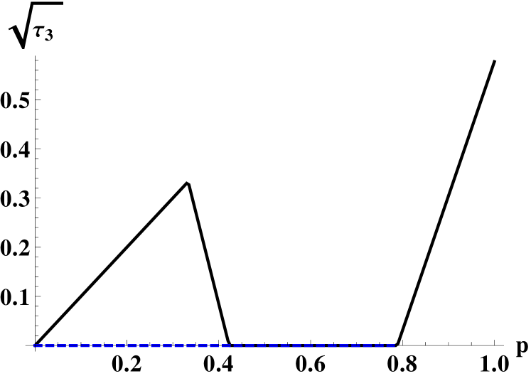
Figure 2: The figure produced by the algorithm (black curve) is shown together with the convexified curve (blue dashed curve), which gives the correct upper bound to the convex roof. It hence is zero up to the value of $p\approx 0.788675$ and begins to linearly increase to finally reach $\sqrt{\tau_{3}}[|\varphi\rangle]=1/\sqrt{3}$. At the value of $p=3/4$ it is hence zero, confirming the result of Ref. Eltschka and Siewert (2014). The minimal value of $p\approx 0.788675$ is a result of this work.

The square-root of the threetangle of this state vanishes at least until $p\approx 0.788675$. The upper bound then consequently linearly increases up to the value of $\sqrt{\tau_{3}}[|\varphi\rangle]=1/\sqrt{3}$. At the value of $p=3/4<0.788675$ it is hence zero, confirming this result of Ref. Eltschka and Siewert (2014).

The next benchmark states are the generalized Werner statesWerner (1989); Murao et al. (1998) including the three-qubit $GHZ$ state

$$\rho_{GHZ,{\rm Werner}}=p\,\pi_{|GHZ\rangle}+\frac{1-p}{8}{\rm 1\kern-2.20001ptl}\;.$$ (22)

Also here, an application of the algorithm to an obvious eigenbasis of $\rho_{GHZ,{\rm Werner}}$ gives a simple straight line connecting $\sqrt{\tau_{3}}[|GHZ\rangle]=1$ at $p=1$ with $0$ at $p=0$. However, we can also here modify the eigenbasis in that it contains $W$-states whose coefficients are suitable zeros of $z^{3}=1$. The result is shown in fig. 3.

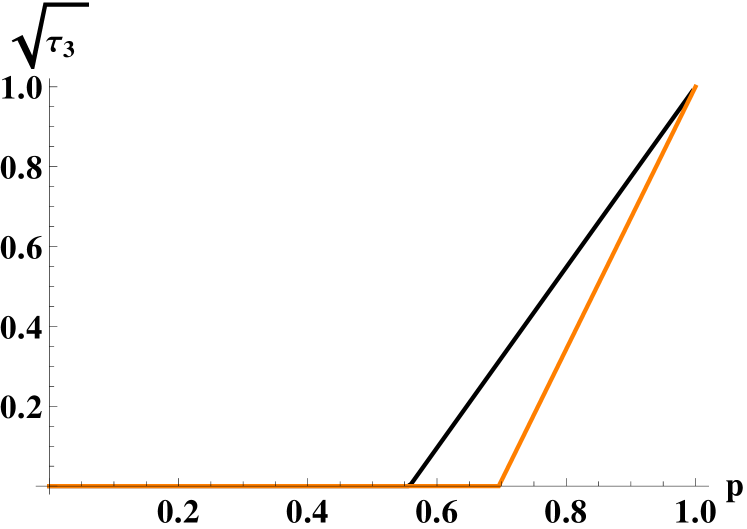
Figure 3: The figure produced by the algorithm (upper black curve) for the modified basis is shown together with the convex roof of $\sqrt{\tau_{3}}$ (lower orange curve)Siewert and Eltschka (2012).

It definitely overestimates the threetangle in the state, but offers an upper bound that vanishes until $p_{0}\approx 0.55750$, whereas the exact value is $p_{0}\approx 0.69554$. The correct decomposition vectors of $\rho_{GHZ,{\rm Werner}}$ are made out of all of its eigenstatesSiewert and Eltschka (2012). They could be seen in an extension of this algorithm to include up to three states in the decomposition.

It is clear that a slight (e.g. experimental) disorder can be dealt with: one has to take the minimum of the eigenvalues in the admixture where we wish to have equal eigenvalues. Then one has

$$\rho=p\,\pi_{\psi}+\Omega_{min}(1-p)\rho_{0}+2\,\delta\!\rho_{0}\approx p\,\pi_{\psi}+(1-p)\rho_{0}$$ (23)

with $\Omega_{min}\lesssim 1$, $2\,{\rm tr}\;\delta\!\rho_{0}=(1-\Omega_{min})(1-p)$, and

$$\rho_{1}:=\frac{p}{p+\Omega_{min}(1-p)}\pi_{\psi}+\frac{\Omega_{min}(1-p)}{p+\Omega_{min}(1-p)}\rho_{0}\;.$$ (24)

If the eigenstates in the degenarate $\rho_{0}$ do not carry entanglement, then one is left with $E[\rho]\leq(p+\Omega_{min}(1-p))E[\rho_{1}]$.

IV Upper bound for the Ising model

In order to demonstrate the algorithm at work, we face towards an upper bound for the threetangle in the Ising model in a transverse field

$$H_{\rm Ising}=\sum_{i}(2\lambda S_{i}^{x}S_{i+1}^{x}+S_{i}^{z})\;,$$ (25)

where the spin matrices $S_{i}^{a}=\sigma_{i}^{a}/2$ for $a=x,z$ enter, and $\lambda$ is a dimension-less interaction parameter; $\sigma^{a}$ are the Pauli matrices. Periodic boundary conditions are imposed and the model is considered in the thermodynamic limit. It has a quantum phase transition at $\lambda=1$. For the ground state of this integrable modelPfeuty (1970); Lieb et al. (1961), I use the expressions for the expectation values Hofmann et al. (2014) to calculate the upper bound to the nearest neighbor (adjacent sites) threetangle $\sqrt{\tau_{3}}$ given by this algorithm. The result can be seen in fig. 4.

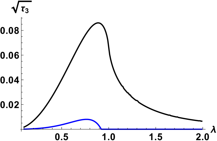
Figure 4: The upper bound coming out of the proposed algorithm is shown for the transverse quantum Ising model as a function of $\lambda$. I have furthermore calculated the lower bound of Ref. Eltschka and Siewert (2014). It is non-zero only for $0\leq\lambda\lesssim 0.9206$ and stays considerably below the upper bound. Form $\lambda>0.9206$ it is zero. In particular, it is also the trivial lower bound in the vicinity of the critical point $\lambda=1$.

The curve has, except the smaller range, an astonishing similarity to the nearest neighbor concurrenceOsterloh et al. (2002); Osborne and Nielsen (2002): it has a maximum which is situated at about $\lambda=0.9$ and decays to zero for $\lambda\to\infty$. With the genuine three party negativityHofmann et al. (2014), which measures besides the $GHZ$ entanglement the non-biseparable $W$ entanglement, also the magnitude is in the same range of $\sqrt{\tau_{3}}\sim 0.09$. I also calculated the lower bound of Ref. Eltschka and Siewert (2014), which is positive but stays cosiderably below the upper bound for $0\leq\lambda\lesssim 0.9206$. For $\lambda>0.9206$ it is zero. In particular, it is the trivial lower bound in the vicinity of the critical point $\lambda=1$. So there is no hint towards a finite three-tangle from this lower bound around the quantum critical point. It is highly probable that the eigenstates of the Ising model are too far away from the GHZ symmetric point because I can almost infer from this upper bound a non-zero threetangle because the sum of the six smallest eigenvalues is below $0.029$ for all $\lambda$, and hence much smaller than the detected threetangle. The state with the third-largest weight is biseparable and does not give a considerable decrease regarding the threetangle; considering the sum of the remaining eigenvalues, one ends up with a value which is smaller than $0.0056$ for all $\lambda$. It is furthermore astonishing how well this upper bound fits into the genuine three-partite negativity of neighboring sitesHofmann et al. (2014). Further studies into this direction must clarify these points.

V Conclusions

I have presented an algorithm that calculates an upper bound of $SL$-invariant entanglement measures $E$, exploiting the knowledge for the rank-two case of Refs. Lohmayer et al. (2006); Osterloh et al. (2008). It is straightforward to include in the algorithm decompositions of three or more eigenstates as soon as they are available. It is thereby a method which is easily extendable to more than two states in the decomposition. In part, however, the algorithm already contains three states in the decomposition of the density matrix and suggestions where more states will be necessary. This opens up a method for experimentally testing the content of an arbitrary SL-invariant entanglement measure, as the threetangle, in the given states.

I demonstrate the algorithm on various benchmark states for three qubits, where the exact convex roof is known Siewert and Eltschka (2012); Eltschka and Siewert (2014). To this end, a modification of the eigenbasis of the states is shown to be obligatory in order to give a reasonable result. This modification is shown to be stable as far as e.g. small experimental errors are concerned. Whereas for the “nontrivial W-state” from Ref. Eltschka and Siewert (2014) it already is sufficient to express the product basis by a basis of maximally entangled $GHZ$-states, no such form exists for the $GHZ$-Werner state. Here, rewriting the product basis in a basis of $W$-states is not sufficient, since it has an optimal decomposition in which all eight eigenstates of $\rho$ occurSiewert and Eltschka (2012). However, an extension to include up to three eigenstates in the decomposition would be enough to reproduce this result.

For demonstrating how the algorithm works without manipulating the eigenbasis, I show the upper bound it offers for the transverse Ising model. I show also a lower bound following Ref. Eltschka and Siewert (2014), which is positive only for $0\leq\lambda\lesssim 0.9206$. There are however strong hints that there is a non-vanishing threetangle in the transverse Ising model for nearest neighbors which will be close to the upper bound given here.

This might induce many possible directions of future research. One direction would be to think about further lower bounds to admit more than two parameters in the density matrices. Furthermore, one could try to enhance the number of eigenstates in the decomposition and improve the present algorithm.

References

- Wootters (1998) W. K. Wootters, Phys. Rev. Lett. 80, 2245 (1998).
- Uhlmann (2000) A. Uhlmann, Phys. Rev. A 62, 032307 (2000).
- Osterloh and Siewert (2005) A. Osterloh and J. Siewert, Phys. Rev. A 72, 012337 (2005).
- Osterloh and Siewert (2006) A. Osterloh and J. Siewert, Int. J. Quant. Inf. 4, 531 (2006).
- D–oković and Osterloh (2009) D. Ž. D–oković and A. Osterloh, J. Math. Phys. 50, 033509 (2009).
- Lohmayer et al. (2006) R. Lohmayer, A. Osterloh, J. Siewert, and A. Uhlmann, Phys. Rev. Lett. 97, 260502 (2006).
- Osterloh et al. (2008) A. Osterloh, J. Siewert, and A. Uhlmann, Phys. Rev. A 77, 032310 (2008).
- Eltschka et al. (2008) C. Eltschka, A. Osterloh, J. Siewert, and A. Uhlmann, New J. Phys. 10, 043014 (2008).
- Coffman et al. (2000) V. Coffman, J. Kundu, and W. K. Wootters, Phys. Rev. A 61, 052306 (2000).
- Jung et al. (2009) E. Jung, M.-R. Hwang, D. Park, and J.-W. Son, Phys. Rev. A 79, 024306 (2009).
- Shu-Juan et al. (2011) H. Shu-Juan, W. Xiao-Hong, F. Shao-Ming, S. Hong-Xiang, and W. Qiao-Yan, Comm. Theor. Phys. 55, 251 (2011).
- Eltschka and Siewert (2012a) C. Eltschka and J. Siewert, Phys. Rev. Lett. 108, 020502 (2012a).
- Siewert and Eltschka (2012) J. Siewert and C. Eltschka, Phys. Rev. Lett. 108, 230502 (2012).
- Eltschka and Siewert (2014) C. Eltschka and J. Siewert, Phys. Rev. A 89, 022312 (2014).
- Eltschka and Siewert (2012b) C. Eltschka and J. Siewert, Sci. Rep. 2, 902 (2012b).
- Eltschka and Siewert (2013) C. Eltschka and J. Siewert, Quant. Inf. Comp. 13, 210 (2013).
- Rodriques et al. (2014) S. Rodriques, N. Datta, and P. Love, Phys. Rev. A 90, 012340 (2014).
- Jungnitsch et al. (2011) B. Jungnitsch, T. Moroder, and O. Gühne, Phys. Rev. Lett. 106, 190502 (2011).
- (19) A. Osterloh, arXiv:1512.02468.
- Viehmann et al. (2012) O. Viehmann, C. Eltschka, and J. Siewert, Appl. Phys. B 106, 533 (2012), spring Meeting of the German-Physical-Society, Dresden, GERMANY, 2011.
- Werner (1989) R. F. Werner, Phys. Rev. A 40, 4277 (1989).
- Murao et al. (1998) M. Murao, M. B. Plenio, S. Popescu, V. Vedral, and P. L. Knight, Phys. Rev. A 57, R4075 (1998).
- Pfeuty (1970) P. Pfeuty, Ann.Phys. 57, 79 (1970).
- Lieb et al. (1961) E. Lieb, T. Schultz, and D. Mattis, Ann. Phys. 16, 407 (1961).
- Hofmann et al. (2014) M. Hofmann, A. Osterloh, and O. Gühne, Phys. Rev. B 89, 134101 (2014).
- Osterloh et al. (2002) A. Osterloh, L. Amico, G. Falci, and R. Fazio, Nature 416, 608 (2002).
- Osborne and Nielsen (2002) T. Osborne and M. A. Nielsen, Phys. Rev. A 66, 032110 (2002).